Quantum Potential Games, Replicator Dynamics, and the Separability Problem

Abstract

Gamification is an emerging trend in the field of machine learning that presents a novel approach to solving optimization problems by transforming them into game-like scenarios. This paradigm shift allows for the development of robust, easily implementable, and parallelizable algorithms for hard optimization problems. In our work, we use gamification to tackle the Best Separable State (BSS) problem, a fundamental problem in quantum information theory that involves linear optimization over the set of separable quantum states. To achieve this we introduce and study quantum analogues of common-interest games (CIGs) and potential games where players have density matrices as strategies and their interests are perfectly aligned. We bridge the gap between optimization and game theory by establishing the equivalence between KKT (first-order stationary) points of a BSS instance and the Nash equilibria of its corresponding quantum CIG. Taking the perspective of learning in games, we introduce non-commutative extensions of the continuous-time replicator dynamics and the discrete-time Baum-Eagon/linear multiplicative weights update for learning in quantum CIGs, which also serve as decentralized algorithms for the BSS problem. We show that the common utility/objective value of a BSS instance is strictly increasing along trajectories of our algorithms, and finally corroborate our theoretical findings through extensive experiments.

1 Introduction

The framework of gamification has recently emerged as a prominent trend in the field of machine learning, offering a novel approach to solving hard optimization problems. By reframing these problems as games, it is possible to design distributed and decentralized algorithms that are robust and easily parallelizable. A notable application of this approach are the constrained min-max optimization problems that underlie Generative Adversarial Networks (GANs), which are known to be computationally challenging [18]. However, by framing them as competitive games between two players, simple decentralized algorithms have been developed, showcasing practical effectiveness and convergence towards appropriate solution concepts. Furthermore, gamification has showcased success in addressing other optimization problems in machine learning such as Principal Component Analysis [26] and Nonnegative Matrix Factorization [68]. While the best-known achievements are based on zero-sum games [16, 17, 55, 67], the current focus is increasingly shifting towards the more challenging domain of cooperative settings [7, 46, 69], where all agents share the same goals and try to optimize the same function.

In this work, we adopt the gamification paradigm to develop distributed algorithms for solving the Best Separable State problem (BSS). The BSS problem corresponds to linear optimization over the convex hull of bipartite product states $\rho\otimes\sigma$, i.e.,

$$\max\{\Tr(R(\rho\otimes\sigma)):\rho\in D(\mathcal{A}),\sigma\in D(\mathcal{B})\}$$ (BSS)

where $R$ is a fixed Hermitian matrix. The BSS problem is a crucial challenge in quantum information theory that is closely tied to entanglement detection [28, 39, 29, 27].

A powerful approach to approximating the BSS problem is to identify outer approximations to the set of separable states over which linear optimization is efficient. These outer approximations typically arise from necessary conditions that are satisfied by separable states. An important example is the Positive Partial Transpose (PPT) criterion for separability [60, 36], stating that a necessary condition for $\rho$ to be separable is that the partial transpose $\rho^{T_{\mathcal{B}}}$ (or $\rho^{T_{\mathcal{A}}}$) is positive semidefinite. Consequently, the value of the BSS problem can be upper bounded by solving a semidefinite programming (SDP) problem. This approach was further extended to the DPS hierarchy [21], a sequence of outer SDP approximations that converges to the set of separable states, and whose first level corresponds to the PPT criterion. A more general problem with many important applications in quantum information theory is the problem of bilinear optimization over density matrices subject to affine constraints, and similar to the DPS hierarchy there exist hierarchies of outer SDP approximations for problems of this type, e.g., see [10, 9]. A complementary approach for solving such problems is a non-commutative extension of the branch-and-bound algorithm [37].

Existing approaches to the BSS problem assume prior knowledge of the matrix $R$ and carry out the computation of a solution in a centralized manner. In this work, we propose decentralized algorithms for the BSS problem that operate in a setting where the matrix $R$ is unknown and the quantum states $\rho,\sigma$ are updated in a decentralized manner using first-order feedback $\nabla_{\rho}\Tr(R(\rho\otimes\sigma))$ and $\nabla_{\sigma}\Tr(R(\rho\otimes\sigma))$ respectively. To achieve this, we reinterpret the BSS problem as a quantum common-interest game (CIG) where the two players have density matrices $\rho,\sigma$ as strategies and share a common bilinear utility function $\Tr(R(\rho\otimes\sigma))$. Building on the existing literature on learning in classical CIGs, we develop dynamics for learning in quantum CIGs. These dynamics lead to equilibration as each agent implements a strategy revision mechanism based on past interactions. Importantly, we also establish the equivalence between KKT points of a BSS instance and Nash equilibria of the corresponding game. By leveraging this equivalence, the learning dynamics for the quantum common-interest game yield robust, easily implementable, and parallelizable decentralized algorithms for the BSS problem.

Classical games and learning dynamics.

In classical game theory, players select strategies from their strategy set and attain utilities that are functions of all players’ strategies. A simple but extremely useful class of games is that of the (classical) normal-form game [25], where each player has a finite strategy set. Specifically in a two-player classical normal-form game, two players whom we call Alice and Bob have strategy sets $S_{\mathcal{A}}=\{1,2,\ldots,n\}$ and $S_{\mathcal{B}}=\{1,2,\ldots,m\}$ and attain the respective utilities $u_{\mathcal{A}}(i,j)$ and $u_{\mathcal{B}}(i,j)$ whenever Alice plays strategy $i$ and Bob plays strategy $j$. Since Alice and Bob can randomize over their respective sets of pure actions, we can more generally consider the mixed extension of the game, where Alice plays a probability distribution (i.e., a probability simplex vector) $x\in\triangle^{n-1}:=\{x\in\mathbb{R}_{\geq 0}^{n}:x_{i}\geq 0\;\forall\ i,\;\sum_{i}x_{i}=1\}$ and Bob plays a probability distribution $y\in\triangle^{m-1}$, and they receive bilinear utilities $u_{\mathcal{A}}(x,y)=x^{\top}Ay$ and $u_{\mathcal{B}}(x,y)=x^{\top}By$ respectively, where $A$ and $B$ are $n\times m$ matrices with $A_{ij}=u_{\mathcal{A}}(i,j)$ and $B_{ij}=u_{\mathcal{B}}(i,j)$.

Potential games are a class of games where a potential function tracks each player’s change in utility due to unilateral deviations, and include Cournot competition [54], congestion games [62], and various other theoretical and engineering applications, see e.g. [50, 75, 31, 19]. An important special class of potential games are common-interest games (CIGs) [65], where players share the same utility function. CIGs are relevant to the study of potential games, since for every potential game there exists a CIG with the same Nash equilibria, and for which players using the same first-order dynamics (i.e., dynamics where each player only gets to see the gradient of the utility with respect to his strategies) would have the same trajectories. Several natural first-order learning dynamics converge to various notions of equilibria, see e.g. [35, 33, 47]. A well-studied first-order continuous-time dynamic are the replicator dynamics. For a two player CIG where players select simplex vectors $x,y$ and receive common payoff $x^{\top}Ay$, the replicator dynamics (written only for the $x$-player) are given by the differential equation:

$$\dot{x}_{i}=x_{i}((Ay)_{i}-x^{\top}Ay),$$ (lin-REP)

or via the equivalent closed-form formulation:

$$x_{i}={\exp(s_{i}(t))\over\sum_{i}\exp(s_{i}(t))},\quad s_{i}(t)=\int_{0}^{t}(Ay(\tau))_{i}d\tau,$$ (exp-REP)

see e.g. [70, 35, 12, 72]. In terms of properties, replicator dynamics converge to Nash equilibria in CIGs [35, 47] and are a gradient flow with respect to the Shahshahani metric $\langle v,w\rangle_{x}=\sum_{i}{\frac{1}{x_{i}}}v_{i}w_{i}$ [66].

There are three related discrete-time dynamics, the latter two of which have an adjustable stepsize $\epsilon>0$:

$$x_{i} \leftarrow x_{i}{(Ay)_{i}\over x^{\top}Ay},$$ (BE)

$$x_{i} \leftarrow x_{i}{1+\epsilon(Ay)_{i}\over\sum_{i}x_{i}(1+\epsilon(Ay)_{i})},$$ (lin-MWU)

$$x_{i} \leftarrow x_{i}{\exp(\epsilon(Ay)_{i})\over\sum_{i}x_{i}\exp(\epsilon(Ay)_{i})}.$$ (exp-MWU)

These discrete-time dynamics are referred to respectively as the Baum-Eagon update [8], the linear multiplicative weights update, and the exponential multiplicative weights update, see e.g.,  [34, 4, 58, 23]. BE and lin-MWU are discrete versions of the lin-REP form of the replicator dynamics in the sense that, in both cases, the weight of a strategy is updated according to how much it performs compared to the average performance $x^{\top}Ay$, and in particular is increased if the strategy does better than average, and decreased if it does worse; on the other hand, exp-MWU is a very natural discretization of the exp-REP formulation of the replicator dynamics in the sense that it is simply exp-REP written recursively for the case where the payoffs are seen at discrete times.

In terms of properties, it is known that the utility function $x^{\top}Ay$ under both BE and lin-MWU is non-decreasing [8], and the limit points of lin-MWU are Nash equilibria [58]. Moreover, stability analysis has shown that replicator dynamics and its discretizations typically converge to pure (i.e., non-randomized) equilibria in generic common-interest games [47, 51, 59]. Table 1 summarizes the relationships between the aforementioned learning dynamics in classical normal-form games.

Variant	Continuous-time	Discrete-time
Linear	lin-REP : $\dot{x}_{i}=x_{i}((Ay)_{i}-x^{\top}Ay)$	BE :   $x_{i}\leftarrow x_{i}{(Ay)_{i}\over x^{\top}Ay}$ lin-MWU :  $x_{i}\leftarrow x_{i}{1+\epsilon(Ay)_{i}\over\sum_{i}x_{i}(1+\epsilon(Ay)_{i})}$
Exponential	exp-REP : $x_{i}={\exp(\int_{0}^{t}(Ay(\tau))_{i}d\tau)\over\sum_{i}\exp(\int_{0}^{t}(Ay(\tau))_{i}d\tau)}$	exp-MWU :  $x_{i}\leftarrow x_{i}{\exp(\epsilon(Ay)_{i})\over\sum_{i}x_{i}\exp(\epsilon(Ay)_{i})}$

Table 1: Relationships between learning dynamics for classical normal-form games. Note that lin-REP and exp-REP are just different expressions of the same replicator dynamic.

Finally, there is an interesting link between classical CIGs and bilinear optimization over the product of simplices. As both agents in a classical CIG are maximizing the same utility function, there is a natural connection between the game (with common payoff matrix $A$) and the bilinear optimization problem $\max\{x^{\top}Ay:x\in\Delta(\mathcal{A}),y\in\Delta(\mathcal{B})\}$. Specifically, the optimization problem’s KKT points correspond to Nash equilibria of the game [65].

Quantum games and learning dynamics.

The majority of the literature on quantum games investigates the potential advantages of using quantum strategies over classical ones. To this end, researchers have developed quantum versions of well-known games such as the Prisoner’s Dilemma [22] and Matching Pennies [53]. In addition, an increasing amount of research has focused on studying quantum notions of equilibria, i.e., states that remain stable against unilateral player deviations [76], determining their tractability [13], and obtaining structural characterizations of equilibrium sets [38]. Beyond the analysis of specific games, various attempts have been made to establish more general theories of quantum games that aim to unify the existing works, see e.g., [30, 15].

In contrast, there are relatively few works that investigate learning in quantum games. Most existing results focus on the zero-sum regime, where players select density matrices $\rho$ and $\sigma$ and receive a bilinear utility $u_{i}(\rho,\sigma)=\text{Tr}(R_{i}(\rho\otimes\sigma))$, subject to the constraint that $u_{1}(\rho,\sigma)+u_{2}(\rho,\sigma)=0$. The payoffs can also be expressed explicitly as bilinear functions $u_{i}(\rho,\sigma)=\langle\rho,\Phi_{i}(\sigma)\rangle$, where $R_{i}$ is the Choi matrix of the superoperator $\Phi_{i}$. The Matrix Multiplicative Weights Update (written only from the perspective of the $\rho$ player) is given by:

$$\rho(t+1)\leftarrow\frac{\exp\left(\epsilon\sum_{\tau=1}^{t}\Phi(\sigma(\tau))\right)}{\Tr(\exp\left(\epsilon\sum_{\tau=1}^{t}\Phi(\sigma(\tau))\right))},$$ (MMWU)

and converges (in the time-average sense) to Nash equilibria in quantum zero-sum games [42]. MMWU was first introduced for online optimization over the set of density matrices [4, 45, 71]. MMWU has found many other applications: important examples include solving SDPs [5], proving that QIP=PSPACE [40], finding balanced separators [57], and spectral sparsification [2].

Recently, [41] introduced the exponential quantum replicator dynamics (exp-QREP), a (continuous-time) quantum analogue of the exp-REP formulation of the replicator dynamics, given by:

$$\rho=\frac{\exp(S(t))}{\mathrm{Tr}(\exp(S(t)))},\quad S(t)=\int_{0}^{t}\Phi(\sigma(\tau))d\tau.$$ (exp-QREP)

Note that these dynamics are simply called the quantum replicator dynamics in [41]. The main result in [41] is that the exp-QREP dynamics exhibit a type of periodic behavior called Poincaré recurrence when applied to quantum zero-sum games. MMWU can be obtained as a discretization of the exp-QREP dynamics, in the same manner the discrete-time update exp-MWU is obtained from the continuous-time dynamics exp-REP in the classical regime. Thus, while non-commutative generalizations of the exponential variants of the classical learning dynamics are known and been studied for learning in quantum games, the linear variants have yet to be studied. In this paper, we complete the picture of analogues of classical replicator and multiplicative update learning dynamics (see Table 2).

	Continuous-time	Discrete-time
Linear variant	3p (this work)	3r, lin-MMWU (this work)
Exponential variant	exp-QREP [41]	MMWU [45, 3, 71]

Table 2: Learning dynamics for quantum games in analogy to those for classical normal-form games in Table 1.

Our results. In Section 2 we introduce quantum common-interest games. We show that any BSS instance can be interpreted as a quantum common-interest game where KKT points corresponds to Nash equilibria. In Sections 3 and 4 respectively we study continuous and discrete-time dynamics for learning in a quantum common-interest game. We show that if players update their states according to any of our dynamics, then the common utility is strictly increasing, limit points are fixed points, and interior fixed points are Nash equilibria. In the same way that the established exp-QREP and MMWU can be viewed as non-commutative extension of exp-REP and exp-MWU respectively, our dynamics can be viewed as noncommutative extensions of lin-REP , BE, and lin-MWU. Finally, in Section 5 we perform extensive experiments to assess the performance of our dynamics. We show that our continuous-time dynamics empirically converges to Nash equilibria, and evaluate our discrete-time algorithms on the BSS problem and show that that they closely approximate the optimal value ($\approx 0.97$ OPT).

2 Quantum Common-Interest Games and the BSS problem

Quantum preliminaries.

A $d$-dimensional quantum register is mathematically described as the set of unit vectors in a $d$-dimensional Hilbert space $\mathcal{H}.$ The state of a qudit quantum register $\mathcal{H}$ is represented by a density matrix, i.e., a $d\times d$ Hermitian positive semidefinite matrix with trace equal to one. The state space of a quantum register $\mathcal{H}$ is denoted by $D(\mathcal{H})$. When two quantum registers with associated spaces $\mathcal{A}$ and $\mathcal{B}$ of dimension $n$ and $m$ respectively are considered as a joint quantum register, the associated state space is given by the density operators on the tensor product space, i.e., $D(\mathcal{A}\otimes\mathcal{B})$. If the two registers are independently prepared in states described by $\rho$ and $\sigma$, then the joint state is described by the density matrix $\rho\otimes\sigma\in\mathbb{C}^{nm\times nm}$.

To interact with a quantum register we need to measure it. One mathematical formalism of the process of measuring a quantum system is the POVM, defined as a set of positive semidefinite operators $\{P_{i}\}_{i=1}^{m}$ such that $\sum_{i=1}^{m}P_{i}=\mathbb{1}_{\mathcal{H}}$, where $\mathbb{1}_{\mathcal{H}}$ is the identity matrix on $\mathcal{H}$. If the quantum register $\mathcal{H}$ is in a state described by density matrix $\rho\in D(\mathcal{H})$, upon performing the measurement $\{P_{i}\}_{i=1}^{m}$ we get the outcome $i$ with probability $\langle P_{i},\rho\rangle$, where $\langle A,B\rangle=\Tr(A^{\dagger}B)$ is the Hilbert-Schmidt inner product defined on the linear space of Hermitian matrices. Note that $\langle A,B\rangle$ is a real number for any Hermitian matrices $A$ and $B$, and is non-negative if $A$ and $B$ are positive semidefinite.

Given a finite-dimensional Hilbert space $\mathcal{H}=\mathbb{C}^{n}$, we denote by $\text{L}(\mathcal{H})$ the set of linear operators acting on $\mathcal{H}$, i.e., the set of all $n\times n$ complex matrices over $\mathcal{H}$. A linear operator that maps matrices to matrices, i.e., a mapping $\Phi:\mathrm{L}(\mathcal{B})\to\mathrm{L}(\mathcal{A})$, is called a super-operator. The adjoint super-operator $\Phi^{\dagger}:\mathrm{L}(\mathcal{A})\to\mathrm{L}(\mathcal{B})$ is uniquely determined by the equation $\langle A,\Phi(B)\rangle=\langle\Phi^{\dagger}(A),B\rangle$. A super-operator $\Phi:\mathrm{L}(\mathcal{B})\to\mathrm{L}(\mathcal{A})$ is positive if it maps PSD matrices to PSD matrices. There exists a linear bijection between matrices $R\in\mathrm{L}(\mathcal{A}\otimes\mathcal{B})$ and super-operators $\Phi:\mathrm{L}(\mathcal{B})\to\mathrm{L}(\mathcal{A})$ known as the Choi-Jamiołkowski isomorphism. Specifically, for a super-operator $\Phi$ its Choi matrix is:

$$C_{\Phi}=\sum_{1\leq i,j\leq m}\Phi(E_{i,j})\otimes E_{i,j}\in\mathrm{L}(\mathcal{A}\otimes\mathcal{B}),$$ (1)

where $\{E_{i,j}\}_{i,j=1}^{m}$ is the standard orthonormal basis of $\mathrm{L}(\mathcal{B})=\mathbb{C}^{m\times m}$. Conversely, given an operator $R=\sum_{1\leq i,j\leq m}A_{i,j}\otimes E_{i,j}\in\mathrm{L}(\mathcal{A}\otimes\mathcal{B})$, we can define $\Phi_{R}:\mathrm{L}(\mathcal{B})\to\mathrm{L}(\mathcal{A})$ by setting $\Phi_{R}(E_{i,j})=A_{i,j}$ from which it easily follows that $C_{\Phi_{R}}=R$. Explicitly, we have

$$\Phi_{R}(B)=\mathrm{Tr}_{\mathcal{B}}(R(\mathbb{1}_{\mathcal{A}}\otimes B^{\top})),$$ (2)

where the partial trace $\mathrm{Tr}_{\mathcal{B}}:\mathcal{L}(\mathcal{A}\otimes\mathcal{B})\to\mathcal{L}(\mathcal{A})$ is the unique function that satisfies:

$$\mathrm{Tr}_{\mathcal{B}}(A\otimes B)=A\Tr(B),\ \forall A,B.$$

Moreover, the adjoint map is $\mathrm{Tr}_{\mathcal{B}}^{\dagger}(A)=A\otimes\mathbb{1}_{\mathcal{B}}$. Lastly, a superoperator $\Phi$ is completely positive (i.e., $\mathbb{1}_{m}\otimes\Phi$ is positive for all $m\in\mathbb{N}$) iff the Choi matrix of $\Phi$ is positive semidefinite. In particular, if the Choi matrix of the super-operator $\Phi$ is PSD, it follows that $\Phi$ is positive.

Quantum potential games.

In the setting of quantum games described in the introduction, we introduce the notion of a quantum potential game as follows. For simplicity we restrict ourselves in this work to the case of two-player games, though the definition can easily be extended to any finite number of players. Furthermore, we restrict ourselves to quantum potential games with bilinear potential. We follow standard game theory notation, where for each player $i$ the set $S_{-i}$ refers to the other player’s strategy set.

Definition 2.1 (Quantum potential game).

Let $\mathcal{A},\mathcal{B}$ be finite-dimensional quantum registers, and suppose that ${V:D(\mathcal{A})\times D(\mathcal{B})\to\mathbb{R},\ (\rho,\sigma)\mapsto\Tr(R(\rho\otimes\sigma))}$ for some Hermitian operator $R$. A two-player game where the players have strategy sets $S_{1}=D(\mathcal{A}),S_{2}=D(\mathcal{B})$ and utility functions $u_{i}:S_{1}\times S_{2}\rightarrow\mathbb{R}$ for all players $i\in\{1,2\}$ is called a quantum potential game with potential $V$ if

$$\begin{split}u_{i}(s,s_{-i})-u_{i}(s^{\prime},s_{-i})=V(s,s_{-i})-V(s^{\prime},s_{-i}).\end{split}$$

for all players $i\in\{1,2\}$, $s_{-i}\in S_{-i}$, and $s,s^{\prime}\in S_{i}.$

Quantum potential games fall into the general class of potential games and so admit an equivalent characterization of coordination-dummy separability (see, e.g., [48]): each player’s utility can be separated into a coordination term (which is the same for all players and equal to the potential $V$) and a dummy term (that only depends on the other players), i.e.,

$$u_{i}(s)=V(s)+D_{i}(s_{-i}).$$

Due to coordination-dummy separation, for each player $i$ the gradients of $u_{i}(s)$ and $V(s)$ with respect to their own strategy are equal. Thus, the trajectories that players’ strategies take under first-order learning dynamics will be the same whether the players play the potential game or the CIG where each player receives utility $V$.

For a two-player game with players Alice and Bob having access to quantum registers $\mathcal{H}_{1}=\mathcal{A}$ and $\mathcal{H}_{2}=\mathcal{B}$ respectively, we can define Alice’s best response set to Bob’s strategy $\sigma\in D(\mathcal{B})$ by $\mathrm{BR}_{\mathcal{A}}(\sigma)=\{\rho\in D(\mathcal{A}):u(\rho,\sigma)\geq u(\rho^{\prime},\sigma)\;\forall\;\rho^{\prime}\in D(\mathcal{A})\}$, and analogously for Bob. The Nash equilibria (NE) of the game are the strategy profiles $(\rho,\sigma)\in D(\mathcal{A})\times D(\mathcal{B})$ such that Alice’s and Bob’s strategies are best responses to each other, i.e.

$$u(\rho,\sigma)\geq u(\rho^{\prime},\sigma),\quad\;\forall\;\rho^{\prime}\in D(\mathcal{A})$$

and

$$\ u(\rho,\sigma)\geq u(\rho,\sigma^{\prime}),\quad\;\forall\;\sigma^{\prime}\in D(\mathcal{B}).$$

Lastly, a Nash equilibrium $(\rho,\sigma)$ is called interior if both $\rho$ and $\sigma$ are positive definite.

The set of Nash equilibria in a quantum potential game with potential $V$ is equivalent to the set of Nash equilibria in the quantum common-interest game with common utility $V$ since, by coordination-dummy separability, no player can unilaterally improve their own utility if and only if no player can unilaterally improve the potential $V$. Thus, for the purpose of learning Nash equilibria in quantum potential games using first-order dynamics, it suffices to study quantum common-interest games.

Quantum common-interest games.

In a quantum CIG, there are two agents Alice and Bob that control quantum registers $\mathcal{A}$ and $\mathcal{B}$ and their strategies are given by density matrices in $D(\mathcal{A})$ and $D(\mathcal{B})$ respectively. Upon playing strategy profile $(\rho,\sigma)\in\ D(\mathcal{A})\times D(\mathcal{B})$ both players receive a common utility $u(\rho,\sigma)=\langle R,\rho\otimes\sigma\rangle$, where $R$ is a Hermitian matrix that we can assume withoout loss of generality to be positive definite. We refer to the matrix $R$ as the game operator. Equivalently, using the Choi-Jamiołkowski isomorphism defined in (1), it is useful to also express the utility function as $u(\rho,\sigma)=\langle\rho,\Phi(\sigma^{\top})\rangle$, since

$$\langle\rho,\Phi(\sigma^{\top})\rangle =\langle\rho,\mathrm{Tr}_{\mathcal{B}}(R(\mathbb{1}_{\mathcal{A}}\otimes\sigma)\rangle=\langle\rho\otimes\operatorname{\mathbb{1}}_{\mathcal{B}},R(\mathbb{1}_{\mathcal{A}}\otimes\sigma)\rangle=\langle R,\rho\otimes\sigma\rangle,$$

where $R$ is the Choi matrix of $\Phi$. Moreover, as $R$ is PSD it follows that $\Phi$ is positive. In order to simplify notation throughout the rest of the paper, we will drop the transpose from the utility and express it as $u(\rho,\sigma)=\langle\rho,\Phi(\sigma)\rangle$ where appropriate. This can be seen as Bob selecting $\sigma^{\top}$ as his strategy, instead of $\sigma$ as defined before.

A quantum CIG can also be defined as the mixed extension of a game where the players’ pure strategies are complex unit vectors $x\in\mathbb{S}_{\mathbb{C}}^{n-1},y\in\mathbb{S}_{\mathbb{C}}^{m-1}$ and the common utility is biquadratic, i.e., $u(x,y)=(x\otimes y)^{\dagger}R(x\otimes y).$

If the players randomize their play using finitely supported distributions $\mathcal{D}_{\mathcal{A}},\mathcal{D}_{\mathcal{B}}$ over their pure strategy spaces, i.e., $\mathcal{D}_{\mathcal{A}}$ has support $\{x_{i}\}_{i=1}^{k}$ and ${\rm Prob}(x_{i})=\lambda_{i}$ whereas $\mathcal{D}_{\mathcal{B}}$ has support $\{y_{j}\}_{j=1}^{\ell}$ and ${\rm Prob}(y_{j})=\mu_{j}$ , the expected payoff is bilinear in the density matrices $\rho=\sum_{i=1}^{k}\lambda_{i}x_{i}x_{i}^{\dagger}$ and $\sigma=\sum_{j=1}^{\ell}\mu_{j}y_{j}y_{j}^{\dagger}$ as

$$\mathbb{E}[(x\otimes y)^{\dagger}R(x\otimes y)]=\Tr(R(\rho\otimes\sigma)),$$

where expectation is taken over $x\sim\mathcal{D}_{\mathcal{A}}$, $y\sim\mathcal{D}_{\mathcal{B}}$.

Lastly, we show that a classical CIG with common utility $x^{\top}Ay$ where $x\in\Delta_{n},y\in\Delta_{m}$ can be viewed as a quantum CIG. Indeed, consider the quantum CIG with diagonal game operator $R\in\mathbb{R}^{nm\times nm}$ whose diagonal entries are $R_{ij,ij}=A_{ij}$. If we only consider diagonal densities $\rho=\sum_{i=1}^{n}x_{i}e_{i}e_{i}^{\dagger}$ and $\sigma=\sum_{j=1}^{m}y_{j}e_{j}e_{j}^{\dagger}$, it is straightforward to verify that $x^{\top}Ay={\rm Tr}(R(\rho\otimes\sigma))$.

Relation between quantum CIGs and the BSS problem.

In a quantum CIG, Alice and Bob try to jointly maximize their common utility function $u(\rho,\sigma)=\langle\rho,\Phi(\sigma)\rangle$. Analogous to the classical case, there is a strong connection between the NE of the game and the underlying BSS optimization problem. Namely, the KKT points of the BSS problem are precisely the Nash equilibria of a corresponding two player quantum CIG.

Theorem 2.1.

The Nash equilibria of a two-player quantum common-interest game with common utility function $u(\rho,\sigma)=\Tr(R(\rho\otimes\sigma))$ correspond to the KKT points of BSS.

Proof.

We shall prove instead that the Nash equilibria of the (transposed) two-player quantum common-interest game with common utility function $u(\rho,\sigma)=\left\langle\rho,\Phi(\sigma)\right\rangle$ correspond to the KKT points of the transposed BSS problem

$$\max\{\left\langle\rho,\Phi(\sigma)\right\rangle:\rho\in D(\mathcal{A}),\sigma\in D(\mathcal{B})\}.$$ (transposed-BSS)

This correspondence is equivalent to the original correspondence we want to prove since $(\rho,\sigma)$ is a Nash equilibrium of the quantum CIG with common utility $\Tr(R(\rho\otimes\sigma))$ iff $(\rho,\sigma^{\top})$ is a Nash equilibrium of the quantum CIG with common utility $\left\langle\rho,\Phi(\sigma)\right\rangle$, and similarly $(\rho,\sigma)$ is a KKT point of the BSS problem iff $(\rho,\sigma^{\top})$ is a KKT point of the transposed-BSS problem.

Note that $\rho\in D(\mathcal{A})$ if and only if $\left\langle\rho,\operatorname{\mathbb{1}}_{\mathcal{A}}\right\rangle=\Tr\,\rho=1$ and $\rho\succeq 0$, and similarly $\sigma\in D(\mathcal{B})$ if and only if $\left\langle\sigma,\operatorname{\mathbb{1}}_{\mathcal{B}}\right\rangle=\Tr\,\sigma=1$ and $\sigma\succeq 0$. The Lagrangian for the transposed-BSS problem is given by

$$L=\left\langle\rho,\Phi(\sigma)\right\rangle+\lambda(1-\left\langle\rho,\operatorname{\mathbb{1}}_{\mathcal{A}}\right\rangle)+\mu(1-\left\langle\sigma,\operatorname{\mathbb{1}}_{\mathcal{B}}\right\rangle)-\left\langle\Lambda,\rho\right\rangle-\left\langle M,\sigma\right\rangle,$$

where the dual variables satisfy $\Lambda\preceq 0$, $M\preceq 0$. Thus, the KKT conditions for the transposed-BSS problem are

$$[left={\nabla L=0:\empheqlbrace}] =\Phi(\sigma)-\lambda\operatorname{\mathbb{1}}_{\mathcal{A}}-\Lambda=0,$$ (3a)

$$\partialderivative{L}{\sigma} =\Phi^{\dagger}(\rho)-\mu\operatorname{\mathbb{1}}_{\mathcal{B}}-M=0;$$ (3b)

$$[left={\text{primal feasibility:}\empheqlbrace}]\rho \in D(\mathcal{A}),$$ (3da)

$$\sigma \in D(\mathcal{B});$$ (3db)

$$[left={\text{dual feasibility:}\empheqlbrace}]\Lambda \preceq 0,$$ (3ea)

$$M \preceq 0;$$ (3eb)

$$[left={\text{complementary slackness:}\empheqlbrace}]\left\langle\Lambda,\rho\right\rangle=0,$$ (3fa)

$$\left\langle M,\sigma\right\rangle=0.$$ (3fb)

Suppose that $(\rho,\sigma,\lambda,\mu,\Lambda,M)$ is a KKT point of the transposed-BSS problem. We show that $(\rho,\sigma)$ is a Nash equilibrium. Using (3a), for any density matrix $\rho^{\prime}\in D(\mathcal{A})$ we get that

$$\left\langle\rho^{\prime},\Phi(\sigma)\right\rangle=\lambda\left\langle\rho^{\prime},\operatorname{\mathbb{1}}_{\mathcal{A}}\right\rangle+\left\langle\rho^{\prime},\Lambda\right\rangle=\lambda+\left\langle\rho^{\prime},\Lambda\right\rangle\leq\lambda,$$

where the inequality follows since $\rho\succeq 0$ and $\Lambda\preceq 0$ (recall (3ea)). On the other hand, if we take the inner product of (3a) with $\rho$ instead we have that

$$\left\langle\rho,\Phi(\sigma)\right\rangle=\lambda\left\langle\rho,\operatorname{\mathbb{1}}_{\mathcal{A}}\right\rangle+\left\langle\rho,\Lambda\right\rangle=\lambda\left\langle\rho,I\right\rangle=\lambda,$$

where we used the complementary slackness condition $\left\langle\rho,\Lambda\right\rangle=0$ (3fa) . Summarizing, we have that $\left\langle\rho^{\prime},\Phi(\sigma)\right\rangle\leq\lambda=\left\langle\rho,\Phi(\sigma)\right\rangle\;\forall\;\rho^{\prime}\in D(\mathcal{A})$, i.e., $\rho$ is a best response to $\sigma$. Similarly we get that $\sigma$ is a best response to $\rho$, and thus that $(\rho,\sigma)$ is a Nash equilibrium of the corresponding quantum CIG.

Next, suppose that $(\rho,\sigma)\in D(\mathcal{A})\times D(\mathcal{B})$ is a Nash equilibrium of the quantum CIG, and consider the point $(\rho,\sigma,\lambda,\mu,\Lambda,M)$ defined by

$$\begin{gathered}\lambda=\left\langle\rho,\Phi(\sigma)\right\rangle,\quad\mu=\left\langle\rho,\Phi(\sigma)\right\rangle,\\ \Lambda=\Phi(\sigma)-\lambda\operatorname{\mathbb{1}}_{\mathcal{A}},\quad M=\Phi^{\dagger}(\rho)-\mu\operatorname{\mathbb{1}}_{\mathcal{B}}.\end{gathered}$$ (3i)

The primal feasibility constraints (3da) and (3db) are satisfied by construction. Furthermore, (3a) is immediately satisfied by the definition of $\Lambda$ and $\lambda$, and similarly (3b) is satisfied by the definition of $M$ and $\mu$. The complementary slackness condition (3fa) holds since

$$\left\langle\rho,\Lambda\right\rangle=\left\langle\rho,\Phi(\sigma)\right\rangle-\lambda\left\langle\rho,\operatorname{\mathbb{1}}_{\mathcal{A}}\right\rangle=\left\langle\rho,\Phi(\sigma)\right\rangle-\lambda=0,$$

and similarly (3fb) is also satisfied. Finally, since $\rho\in\mathrm{BR}_{\mathcal{A}}(\sigma)$ we have that $\forall\;v\in\mathbb{C}^{m}$ with $\norm{v}_{2}=1$

$$v^{\dagger}\Phi(\sigma)v=\left\langle vv^{\dagger},\Phi(\sigma)\right\rangle\leq\left\langle\rho,\Phi(\sigma)\right\rangle=\lambda,$$

which in turn implies that $\Lambda\preceq 0$ as

$$v^{\dagger}\Lambda v=v^{\dagger}\Phi(\sigma)v-\lambda\norm{v}_{2}^{2}=v^{\dagger}\Phi(\sigma)v-\lambda\leq 0.$$

Thus (3ea) is satisfied and a similar argument shows that (3eb) is also satisfied. ∎

For a classical game, if $(x,y)$ is a Nash equilibrium, every pure strategy that is played by Alice with positive probability is a best response to $y$, i.e., for each $i$ with $x_{i}>0$ we have $(Ay)_{i}=x^{T}Ay$, and similarly for Bob. We now prove the analogous statement for quantum CIGs.

Theorem 2.2.

Let $(\rho,\sigma)$ be a Nash equilibrium of a two-player quantum CIG with common utility $u(\rho,\sigma)=\left\langle\rho,\Phi(\sigma)\right\rangle$. If $\rho\succ 0$, we have that $\Phi(\sigma)=\left\langle\rho,\Phi(\sigma)\right\rangle\operatorname{\mathbb{1}}_{\mathcal{B}}$, i.e., for any $\rho^{\prime}\in D(\mathcal{A})$ we have $\rho^{\prime}\in\mathrm{BR}_{\mathcal{A}}(\sigma).$ Similarly, if $(\rho,\sigma)$ is a Nash equilibrium and $\sigma\succ 0$, then $\Phi^{\dagger}(\rho)=\leavevmode\nobreak\ \left\langle\rho,\Phi(\sigma)\right\rangle\operatorname{\mathbb{1}}_{\mathcal{A}}$.

Proof.

By Theorem 2.1 there exist $\lambda,\mu\in\mathbb{R}$ and Hermitian matrices $\Lambda\in{\mathrm{L}}(\mathcal{A})$, $M\in{\mathrm{L}}(\mathcal{B})$ such that $(\rho,\sigma,\lambda,\mu,\Lambda,M)$ satisfy the KKT conditions (3a)-(3fb). Since $\rho\succ 0$ and $\Lambda\preceq 0$, the complementary slackness condition (3fa) (i.e., $\left\langle\Lambda,\rho\right\rangle=0$) implies that $\Lambda=0$. In turn, the KKT condition (3a) implies that $\Phi(\sigma)=\lambda\operatorname{\mathbb{1}}_{\mathcal{A}}$, i.e., that any density matrix the $\rho$-player can select achieves the same utility $\lambda$ against $\sigma$. But we know that the $\rho$-player attains utility $\left\langle\rho,\Phi(\sigma)\right\rangle$ by selecting the density matrix $\rho$ as her strategy, and so $\Phi(\sigma)=\left\langle\rho,\Phi(\sigma)\right\rangle\operatorname{\mathbb{1}}_{\mathcal{A}}$. The proof that if $(\rho,\sigma)$ is a Nash equilibrium and $\sigma\succ 0$, then $\Phi^{\dagger}(\rho)=\leavevmode\nobreak\ \left\langle\rho,\Phi(\sigma)\right\rangle\operatorname{\mathbb{1}}_{\mathcal{B}}$ is completely symmetric. ∎

With the connection between Nash equilibria and KKT points of the BSS problem established, and motivated by the well-known classical result that ‘natural’ learning dynamics converge to Nash equilibria in classical CIGs, in the next section we propose a non-commutative extension of one such family of gradient flow dynamics and study their theoretical convergence properties.

3 Continuous-time Dynamics

Gradient flow dynamics.

While the implementation of learning in game theory often requires algorithms in discrete time, past work has shown that continuous-time dynamics can give rise to families of discrete dynamics. The most relevant such examples to our work are in the context of gradient-based optimization algorithms [73, 56] and evolutionary game dynamics [52, 66].

Consider a differentiable manifold $\mathcal{M}$ equipped with a differentiable scalar field $u:\mathcal{M}\rightarrow\mathbb{R}$ and a symmetric, positive-definite inner product $\left\langle\cdot,\cdot\right\rangle_{p}:T_{p}\mathcal{M}\times T_{p}\mathcal{M}\rightarrow\leavevmode\nobreak\ \mathbb{R}_{\geq 0}$ defined at all $p\in\mathcal{M}$. (Here $T_{p}\mathcal{M}$ is the tangent space of $\mathcal{M}$ at $p$.) By the Riesz Representation Theorem (see, e.g., [64]), at each $p\in\mathcal{M}$ there exists a unique vector $\textbf{grad}\,u(p)\in T_{p}\mathcal{M}$ with

$$D_{p}u(\xi)=\left\langle\textbf{grad}\,u(p),\xi\right\rangle_{p}\quad\forall\;\xi\in T_{p}\mathcal{M},$$ (3j)

where $D_{p}u(\xi):T_{p}\mathcal{M}\rightarrow\mathbb{R}$ is the directional derivative of $u$ at the point $p$ in direction $\xi$, i.e., $D_{p}u(\xi)\leavevmode\nobreak\ =\leavevmode\nobreak\ \langle\nabla u(p),\xi\rangle$ where $\nabla u(p)$ is the usual Euclidean gradient of $u$ at $p$ and $\langle\cdot,\cdot\rangle$ is the Euclidean inner product. Equation (3j) allows us to associate to each point $p\in\mathcal{M}$ a vector $\textbf{grad}\,u(p)\in\leavevmode\nobreak\ T_{p}\leavevmode\nobreak\ \mathcal{M}$, or in other words, to define a gradient flow on the manifold $\mathcal{M}$ given explicitly by $\dot{p}=\textbf{grad}\,u(p)$. Moreover, simply by construction, it follows that the function $u(p)$ is nondecreasing along the trajectories of the gradient flow, i.e., $\derivative{u(p)}{t}\geq 0$ since $\derivative{u(p)}{t}=\langle\nabla u(p),\dot{p}\rangle=D_{p}u(\dot{p})=\left\langle\textbf{grad}\,u(p),\dot{p}\right\rangle_{p}=\left\langle\dot{p},\dot{p}\right\rangle_{p}\geq 0,$ and moreover $\derivative{u(p)}{t}=0$ if and only if $\dot{p}=0$ (as the inner product $\left\langle\cdot,\cdot\right\rangle_{p}$ is positive definite), so $u$ is in fact strictly increasing along gradient flow trajectories unless at a fixed point.

Quantum Shahshahani gradient flow.

Consider a two-player quantum CIG with common utility $u(\rho,\sigma)=\langle\rho,\Phi(\sigma)\rangle.$ Our goal is to provide continuous-time dynamics that improve the utility $u(\rho,\sigma)$. The state space we are operating in is the manifold $\mathcal{M}\leavevmode\nobreak\ =\leavevmode\nobreak\ D(\mathcal{A})\leavevmode\nobreak\ \times\leavevmode\nobreak\ D(\mathcal{B})$, so all that remains is to select a metric on the manifold of density matrices which would imbue the product manifold $\mathcal{M}$ with the product metric, giving a gradient flow. To accomplish this, we consider the generalized family of Riemannian metrics on the manifold of PSD matrices parametrized by $q\in\mathbb{R}$, which we call the quantum $q$-Shahshahani metric:

$$\left\langle A,B\right\rangle_{\rho}^{(q)}:=\Tr[\rho^{-\frac{q}{2}}A\rho^{-\frac{q}{2}}B].$$ (QShah)

Indeed, in the case of diagonal matrices this family of metrics reduces to the $q$-Shahshahani family of metrics on the simplex (see [52]). On the PSD manifold, $q=0$ gives the Euclidean inner product $\Tr[AB]$, while $q=2$ gives the intrinsic Riemannian metric, e.g. see [11]. In addition, $q=1$ reduces to the Shahshahani metric on the simplex in the case of diagonal matrices.

Theorem 3.1 (Linear quantum $q$-replicator dynamics).

Consider a quantum CIG with utility function $u(\rho,\sigma)=\langle\rho,\Phi(\sigma)\rangle$ where $\rho\in D(\mathcal{A}),\sigma\in D(\mathcal{B})$. The dynamics

$$\begin{gathered}\derivative{\rho}{t}=\rho^{\frac{q}{2}}\left[\Phi(\sigma)-\frac{\Tr[\rho^{q}\Phi(\sigma)]}{\Tr[\rho^{q}]}\operatorname{\mathbb{1}}_{\mathcal{A}}\right]\rho^{\frac{q}{2}},\\ \derivative{\sigma}{t}=\sigma^{\frac{q}{2}}\left[\Phi^{\dagger}(\rho)-\frac{\Tr[\sigma^{q}\Phi^{\dagger}(\rho)]}{\Tr[\sigma^{q}]}\operatorname{\mathbb{1}}_{\mathcal{B}}\right]\sigma^{\frac{q}{2}}\end{gathered}$$ (3l)

define a gradient flow of the utility function $u(\rho,\sigma)$ on the product manifold $D(\mathcal{A})\times D(\mathcal{B})$ imbued with the quantum $q$-Shahshahani metric. Moreover, the utility $u(\rho,\sigma)$ is strictly increasing along the trajectories of the 3l dynamics, except at fixed points.

Proof.

To derive the 3l dynamics as a gradient flow with respect to the quantum $q$-Shahshahani metric $\left\langle A,B\right\rangle_{\rho}^{(q)}:=\Tr[\rho^{-\frac{q}{2}}A\rho^{-\frac{q}{2}}B]$ given in (QShah), we operate on the product manifold $\mathcal{M}=D(\mathcal{A})\times D(\mathcal{B})$ endowed with the product metric and use the scalar field $u:\mathcal{M}\rightarrow\mathbb{R},\;(\rho,\sigma)\mapsto\left\langle\rho,\Phi(\sigma)\right\rangle$ corresponding to the common utility function. At any point $(\rho,\sigma)\in\mathcal{M}$, we want to find ${\bf grad}^{(q)}u(\rho,\sigma)$, defined as the unique vector $g=(g_{\mathcal{A}},g_{\mathcal{B}})\in T_{(\rho,\sigma)}\mathcal{M}=T_{\rho}D(\mathcal{A})\times T_{\sigma}D(\mathcal{B})$ satisfying

$$D_{(\rho,\sigma)}u(\xi_{\mathcal{A}},\xi_{\mathcal{B}})=\langle(g_{\mathcal{A}},g_{\mathcal{B}}),(\xi_{\mathcal{A}},\xi_{\mathcal{B}})\rangle^{(q)}_{(\rho,\sigma)},\ \text{ for all }\xi=(\xi_{\mathcal{A}},\xi_{\mathcal{B}})\in T_{(\rho,\sigma)}\mathcal{M}.$$

Expanding the above we immediately get that

$$D_{(\rho,\sigma)}u(\xi_{\mathcal{A}},\xi_{\mathcal{B}})=\langle g_{\mathcal{A}},\xi_{\mathcal{A}}\rangle^{(q)}_{\rho}+\langle g_{\mathcal{B}},\xi_{\mathcal{B}}\rangle^{(q)}_{\sigma}=\Tr[{\rho}^{-\frac{q}{2}}{g_{\mathcal{A}}}{\rho}^{-\frac{q}{2}}{\xi_{\mathcal{A}}}]+\Tr[{\sigma}^{-\frac{q}{2}}{g_{\mathcal{B}}}{\sigma}^{-\frac{q}{2}}{\xi_{\mathcal{B}}}],$$ (3m)

while on the other hand, as the Euclidean gradient $\nabla u(\rho,\sigma)=\left(\Phi(\sigma),\Phi^{\dagger}(\rho)\right)$, we have that

$$D_{(\rho,\sigma)}u(\xi_{\mathcal{A}},\xi_{\mathcal{B}})=\langle\nabla u(\rho,\sigma),(\xi_{\mathcal{A}},\xi_{\mathcal{B}})\rangle=\Tr[\Phi(\sigma)\xi_{\mathcal{A}}]+\Tr[\Phi^{\dagger}(\rho)\xi_{\mathcal{B}}].$$ (3n)

Equating (3m) and (3n), we then have that ${\bf grad}^{(q)}u(\rho,\sigma)$ is the unique element $(g_{\mathcal{A}},g_{\mathcal{B}})$ in the product of the tangent spaces $T_{\rho}D(\mathcal{A})\times T_{\sigma}D(\mathcal{B})$ with the following properties:

• $g_{\mathcal{A}}$ is the unique element in $T_{\rho}D(\mathcal{A})$ such that

  $$\Tr[{\rho}^{-\frac{q}{2}}{g_{\mathcal{A}}}{\rho}^{-\frac{q}{2}}{\xi_{\mathcal{A}}}]=\Tr[\Phi(\sigma)\xi_{\mathcal{A}}]\quad\forall\;\xi_{\mathcal{A}}\in T_{\rho}D(\mathcal{A}).$$

• $g_{\mathcal{B}}$ is the unique element in $T_{\sigma}D(\mathcal{B})$ such that

  $$\Tr[{\sigma}^{-\frac{q}{2}}{g_{\mathcal{B}}}{\sigma}^{-\frac{q}{2}}{\xi_{\mathcal{B}}}]=\Tr[\Phi^{\dagger}(\rho)]\xi_{\mathcal{B}}\quad\forall\;\xi_{\mathcal{B}}\in T_{\sigma}D(\mathcal{B}).$$

A straightforward computation shows that for any constant $c$ we have

$$\Tr[\Phi(\sigma)\xi_{\mathcal{A}}] =\Tr[(\Phi(\sigma)-c\mathbb{1}_{\mathcal{A}})\xi_{\mathcal{A}}]$$

$$=\Tr[{\rho}^{-\frac{q}{2}}\underbrace{({\rho}^{\frac{q}{2}}(\Phi(\sigma)-c\mathbb{1}_{\mathcal{A}}){\rho}^{\frac{q}{2}})}_{g_{\mathcal{A}}}{\rho}^{-\frac{q}{2}}\xi_{\mathcal{A}}]$$

where for the first equality we used that tangent space of $T_{\rho}D(\mathcal{A})$ consists of traceless matrices. Lastly, to make $g_{\mathcal{A}}$ traceless we need to select the constant $c$ so that

$$\Tr({\rho}^{\frac{q}{2}}(\Phi(\sigma)-c\mathbb{1}_{\mathcal{A}}){\rho}^{\frac{q}{2}})=0\iff c=\frac{\Tr[\rho^{q}\Phi(\sigma)]}{\Tr[\rho^{q}]}.$$

Summarizing, we have established that

$$g_{\mathcal{A}}=\rho^{\frac{q}{2}}\left[\Phi(\sigma)-\frac{\Tr[\rho^{q}\Phi(\sigma)]}{\Tr[\rho^{q}]}I\right]\rho^{\frac{q}{2}}$$

and symmetrically we also get that

$$g_{\mathcal{B}}=\sigma^{\frac{q}{2}}\left[\Phi^{\dagger}(\rho)-\frac{\Tr[\sigma^{q}\Phi^{\dagger}(\rho)]}{\Tr[\sigma^{q}]}I\right]\sigma^{\frac{q}{2}}.$$

Thus, the gradient flow on the product manifold $D(\mathcal{A})\times D(\mathcal{B})$ endowed with the quantum $q$-Shahshahani metric is given by

$$\derivative{\rho}{t}=g_{\mathcal{A}}=\rho^{\frac{q}{2}}\left[\Phi(\sigma)-\frac{\Tr[\rho^{q}\Phi(\sigma)]}{\Tr[\rho^{q}]}I\right]\rho^{\frac{q}{2}},\quad\derivative{\sigma}{t}=g_{\mathcal{B}}=\sigma^{\frac{q}{2}}\left[\Phi^{\dagger}(\rho)-\frac{\Tr[\sigma^{q}\Phi^{\dagger}(\rho)]}{\Tr[\sigma^{q}]}I\right]\sigma^{\frac{q}{2}}.$$

That the utility $u=\left\langle\rho,\Phi(\sigma)\right\rangle$ is strictly increasing unless at fixed points follows directly from the fact that this dynamic is a gradient flow. ∎

In terms of the convergence properties of 3l we have the following result:

Corollary 3.1.

The set of $\omega$-limit points of a trajectory $\{\rho(t),\sigma(t)\}_{t\geq 0}$ of the 3l dynamics is a compact, connected set of fixed points of the dynamics that all attain the same utility.

The proof of this result follows directly from an extension of the fundamental convergence theorem by [49] to general compact sets, which we prove in Theorem LABEL:thm:_LimitSetCompactConnected_ContTime.

Linear quantum replicator dynamics.

For $q=1$, the 3l dynamics specialize to:

$$\begin{gathered}\derivative{\rho}{t}=\rho^{\nicefrac{{1}}{{2}}}\Big{[}\Phi(\sigma)-\left\langle\rho,\Phi(\sigma)\right\rangle\operatorname{\mathbb{1}}_{\mathcal{A}}\Big{]}\rho^{\nicefrac{{1}}{{2}}},\\ \derivative{\sigma}{t}=\sigma^{\nicefrac{{1}}{{2}}}\Big{[}\Phi^{\dagger}(\rho)-\left\langle\rho,\Phi(\sigma)\right\rangle\operatorname{\mathbb{1}}_{\mathcal{B}}\Big{]}\sigma^{\nicefrac{{1}}{{2}}}\end{gathered}$$ (3p)

which we call the linear quantum replicator dynamics. The direction of the 3p dynamics points within the tangent cone of the product of the trace-1 spectrahedra, meaning that trajectories that begin as a product of density matrices remain as a product of density matrices (see Appendix A). We next observe that the 3p dynamics are a non-commutative generalization of the celebrated replicator dynamics [72, 65]: specifically, the 3p dynamics reduce to the usual replicator dynamics when applied to the quantum embedding of a classical CIG with common utility $x^{\top}Ay$. A full explanation of this observation can be found in Appendix LABEL:appsecs:diagonal.

Finally, we relate the interior fixed points and limit points of 3p with Nash equilibria.

Theorem 3.2.

For a quantum CIG with common utility function $u(\rho,\sigma)=\langle\rho,\Phi(\sigma)\rangle$ where $\rho\in D(\mathcal{A}),\sigma\in D(\mathcal{B})$, we have the following two properties relating interior fixed points and $\omega$-limit points of the 3p dynamics with Nash equilibria of the game:

1. The set of interior fixed points of the 3p dynamics is equivalent to the set of interior Nash equilibria.

2. The interior $\omega$-limits of any trajectory of the 3p dynamics are Nash equilbria.

Proof.

$(1)$ By Theorem 2.2, if $(\rho,\sigma)$ is an interior NE of the game, then $\Phi(\sigma)=\left\langle\rho,\Phi(\sigma)\right\rangle\operatorname{\mathbb{1}}_{\mathcal{A}}$ and $\Phi^{\dagger}(\rho)\leavevmode\nobreak\ =\leavevmode\nobreak\ \left\langle\rho,\Phi(\sigma)\right\rangle\operatorname{\mathbb{1}}_{\mathcal{B}}$. This immediately implies that $\dot{\rho}=\rho^{\nicefrac{{1}}{{2}}}\left[\Phi(\sigma)-\left\langle\rho,\Phi(\sigma)\right\rangle\operatorname{\mathbb{1}}_{\mathcal{A}}\right]\rho^{\nicefrac{{1}}{{2}}}=0$ and $\dot{\sigma}\leavevmode\nobreak\ =\leavevmode\nobreak\ \sigma^{\nicefrac{{1}}{{2}}}\left[\Phi^{\dagger}(\rho)-\left\langle\rho,\Phi(\sigma)\right\rangle\operatorname{\mathbb{1}}_{\mathcal{B}}\right]\sigma^{\nicefrac{{1}}{{2}}}\leavevmode\nobreak\ =\leavevmode\nobreak\ 0$, i.e., $(\rho,\sigma)$ is a fixed point of the 3p dynamics. Conversely, let $(\rho,\sigma)$ be an interior fixed point of the 3p dynamics. As $\rho$ is invertible and $\dot{\rho}=0$ we immediately get that $\Phi(\sigma)=\left\langle\rho,\Phi(\sigma)\right\rangle\operatorname{\mathbb{1}}_{\mathcal{A}}.$ In turn, this implies that $\rho\in\mathrm{BR}_{\mathcal{A}}(\sigma)$ and similarly, $\sigma\in\mathrm{BR}_{\mathcal{B}}(\rho)$. Thus, $(\rho,\sigma)$ is an interior NE.

$(2)$ By Corollary 3.1, all $\omega$-limits of any trajectory of the 3p dynamics are fixed points. But as we have just proven, interior fixed points are Nash equilibria. ∎

4 Discrete-time Dynamics

Consider a quantum common-interest game with utility $u(\rho,\sigma)=\left\langle\rho,\Phi(\sigma)\right\rangle,$ where the Choi matrix $R$ corresponding to the superoperator $\Phi$ is strictly positive. We introduce the following two dynamics:

Matrix Baum-Eagon update.

We first study a discretization of the 3p dynamics given by

$$\begin{gathered}{\rho}^{new}\leftarrow\frac{1}{\left\langle\rho,\Phi(\sigma)\right\rangle}\rho^{\nicefrac{{1}}{{2}}}\Phi(\sigma)\rho^{\nicefrac{{1}}{{2}}},\\ {\sigma}^{new}\leftarrow\frac{1}{\left\langle{\rho}^{new},\Phi(\sigma)\right\rangle}\sigma^{\nicefrac{{1}}{{2}}}{\Phi}^{\dagger}({\rho}^{new})\sigma^{\nicefrac{{1}}{{2}}}\end{gathered}$$ (3r)

which we call the Matrix Baum-Eagon update. 3r is defined in an alternating manner (i.e., $\rho$ and $\sigma$ are updated in turn) and only uses first-order information (i.e., to perform the update, each agent only needs to know the gradient of the utility with respect to their own density). Moreover, 3r is a non-commutative extension of BE in the sense that 3r reduces to BE when the game operator is diagonal and $\rho,\sigma$ are diagonal densities. Indeed, define the diagonal game operator $R_{ij,ij}=A_{ij}$, and consider diagonal density matrices $\rho=\sum_{\ell}x_{\ell}e_{\ell}e_{\ell}^{\dagger}$ and $\sigma=\sum_{k}y_{k}f_{k}f_{k}^{\dagger}$. By (LABEL:diag) we have $\Phi(\sigma)={\rm diag}(Ay).$ Thus,

$${\rho}^{new}=\frac{1}{\left\langle\rho,\Phi(\sigma)\right\rangle}\rho^{\nicefrac{{1}}{{2}}}\Phi(\sigma)\rho^{\nicefrac{{1}}{{2}}}={1\over x^{\top}Ay}{\rm diag}(x\circ(Ay)),$$

where $\circ$ denotes the componentwise vector product.

For 3r to be well defined, we need the game operator $R$ to be positive definite. Indeed, when applied to $(\rho,\sigma)\in D(\mathcal{A})\times D(\mathcal{B})$, the update ${\rho}^{new}$ is also a density matrix as $\rho^{1/2}\Phi(\sigma)\rho^{1/2}$ is PSD (as $R$ is PSD and thus $\Phi$ is positive) and the scalar $\left\langle\rho,\Phi(\sigma)\right\rangle$ is also strictly positive (as $\left\langle\rho,\Phi(\sigma^{\top})\right\rangle=\langle R,\rho\otimes\sigma\rangle$ and $R$ is positive definite and $\rho\otimes\sigma^{\top}$ is PSD). Lastly, using the cyclic property of the trace, clearly the update ${\rho}^{new}$ has trace equal to one.

Linear Matrix Multiplicative Weights Update.

3r is an extension of the classical Baum-Eagon update, but we can also define the non-commutative extension of lin-MWU (as studied in [58]). In order to improve the practicality of 3r, we introduce Linear Matrix Multiplicative Weights Update (lin-MMWU), which can be viewed as a more tunable version of 3r that incorporates a stepsize, given by

$$\begin{split}{\rho}^{new}&\leftarrow\frac{\rho^{\nicefrac{{1}}{{2}}}[\operatorname{\mathbb{1}}_{\mathcal{A}}+\epsilon\Phi(\sigma)]\rho^{\nicefrac{{1}}{{2}}}}{1+\epsilon\left\langle\rho,\Phi(\sigma)\right\rangle},\\ {\sigma}^{new}&\leftarrow\frac{\sigma^{\nicefrac{{1}}{{2}}}[\operatorname{\mathbb{1}}_{\mathcal{B}}+\epsilon\Phi^{\dagger}({\rho}^{new})]\sigma^{\nicefrac{{1}}{{2}}}}{1+\epsilon\left\langle{\rho}^{new},\Phi(\sigma)\right\rangle}.\end{split}$$ (lin-MMWU)

Here $\epsilon>0$ is the adjustable stepsize (lin-MMWU becomes 3r in the limit $\epsilon\to\infty$). lin-MMWU only uses first-order information and is defined in a alternating manner (i.e., $\rho$ and $\sigma$ are updated in turn). Morever, lin-MMWU is a non-commutative extension of lin-MWU in the sense that lin-MMWU reduces to lin-MWU when the game operator is diagonal and $\rho,\sigma$ are diagonal densities. It should be noted that for the lin-MMWU dynamics to be well defined it suffices that $\Phi\succ-\frac{\operatorname{\mathbb{1}}}{\epsilon}$, but we shall nevertheless keep the stronger assumption of strict positivity for ease of stating results for 3r and lin-MMWU concurrently.

Properties of discrete-time dynamics.

We now show that the utility is increasing under both the discrete-time 3r and lin-MMWU updates, as it was along trajectories of the continuous-time 3p dynamics.

Theorem 4.1.

Suppose that the two players playing a quantum CIG with a positive definite game operator $R$ update their strategies according to either 3r or lin-MMWU. Then the common utility $u(\rho,\sigma)=\left\langle\rho,\Phi(\sigma)\right\rangle$ is strictly increasing under each unilateral update, except when the update does nothing. In particular, the common utility is strictly increasing under a round of sequential updates unless the strategy profile is a fixed point.

Proof.

We first note that for density matrices $\rho,\sigma$ we have that

$$\left\langle\rho^{\nicefrac{{1}}{{2}}}\Phi(\sigma)\rho^{\nicefrac{{1}}{{2}}},\Phi(\sigma)\right\rangle\geq\left\langle\rho,\Phi(\sigma)\right\rangle^{2}$$ (3s)

with equality iff $\rho^{\nicefrac{{1}}{{2}}}\Phi(\sigma)\rho^{\nicefrac{{1}}{{2}}}$ is a scaling of $\rho$, and similarly

$$\left\langle\rho,\Phi\left(\sigma^{\nicefrac{{1}}{{2}}}\Phi^{\dagger}(\rho)\sigma^{\nicefrac{{1}}{{2}}}\right)\right\rangle\geq\left\langle\rho,\Phi(\sigma)\right\rangle^{2}$$ (3t)

with equality iff $\sigma^{\nicefrac{{1}}{{2}}}\Phi^{\dagger}(\rho)\sigma^{\nicefrac{{1}}{{2}}}$ is a scaling of $\sigma$. This is because setting $\norm{A}=\sqrt{\left\langle A,A\right\rangle}$, we have that

$$\left\langle\rho^{\nicefrac{{1}}{{2}}}\Phi(\sigma)\rho^{\nicefrac{{1}}{{2}}},\Phi(\sigma)\right\rangle=\norm{\rho^{\nicefrac{{1}}{{4}}}\Phi(\sigma)\rho^{\nicefrac{{1}}{{4}}}}^{2}=\norm{\rho^{\nicefrac{{1}}{{4}}}\Phi(\sigma)\rho^{\nicefrac{{1}}{{4}}}}^{2}\norm{\rho^{\nicefrac{{1}}{{2}}}}^{2}\geq\left\langle\rho^{\nicefrac{{1}}{{4}}}\Phi(\sigma)\rho^{\nicefrac{{1}}{{4}}},\rho^{\nicefrac{{1}}{{2}}}\right\rangle^{2}=\left\langle\rho,\Phi(\sigma)\right\rangle^{2},$$

where the inequality is due to Cauchy-Schwarz and the fact that $\norm{\rho^{\nicefrac{{1}}{{2}}}}^{2}=\tr(\rho)=\leavevmode\nobreak\ 1$. Moreover, equality holds iff $\rho^{\nicefrac{{1}}{{4}}}\Phi(\sigma)\rho^{\nicefrac{{1}}{{4}}}$ is a scaling of $\rho^{\nicefrac{{1}}{{2}}}$. But if $\rho^{\nicefrac{{1}}{{4}}}\Phi(\sigma)\rho^{\nicefrac{{1}}{{4}}}=c\rho^{\nicefrac{{1}}{{2}}}$ for some $c\in\mathbb{R}$, then $\rho^{\nicefrac{{1}}{{2}}}\Phi(\sigma)\rho^{\nicefrac{{1}}{{2}}}=\rho^{\nicefrac{{1}}{{4}}}(\rho^{\nicefrac{{1}}{{4}}}\Phi(\sigma)\rho^{\nicefrac{{1}}{{4}}})\rho^{\nicefrac{{1}}{{4}}}=\rho^{\nicefrac{{1}}{{4}}}(c\rho^{\nicefrac{{1}}{{2}}})\rho^{\nicefrac{{1}}{{4}}}=c\rho$, and conversely if $\rho^{\nicefrac{{1}}{{2}}}\Phi(\sigma)\rho^{\nicefrac{{1}}{{2}}}=c\rho$, then letting $Q:=\sum_{i}f(\lambda_{i})v_{i}v_{i}^{\dagger}$ where $\rho^{\nicefrac{{1}}{{4}}}$ has spectral decomposition $\sum_{i}\lambda_{i}v_{i}v_{i}^{\dagger}$ and $f:\mathbb{R}_{\geq 0}\rightarrow\mathbb{R}_{\geq 0},\;f:x\mapsto\begin{cases}x^{-1}\quad\text{if }x>0\\ 0\qquad\text{if }x=0\end{cases}$, we have that $\rho^{\nicefrac{{1}}{{4}}}\Phi(\sigma)\rho^{\nicefrac{{1}}{{4}}}=Q\rho^{\nicefrac{{1}}{{2}}}\Phi(\sigma)\rho^{\nicefrac{{1}}{{2}}}Q=cQ\rho Q=c\rho^{\nicefrac{{1}}{{2}}}$. Thus equality holds iff $\rho^{\nicefrac{{1}}{{2}}}\Phi(\sigma)\rho^{\nicefrac{{1}}{{2}}}$ is a scaling of $\rho$, and inequality (3t) and its equality condition can be similarly obtained.

Thus, under a $\rho$-update of 3r, we have that

$$\left\langle{\rho}^{new},\Phi(\sigma)\right\rangle=\frac{1}{\left\langle\rho,\Phi(\sigma)\right\rangle}\left\langle\rho^{\nicefrac{{1}}{{2}}}\Phi(\sigma)\rho^{\nicefrac{{1}}{{2}}},\Phi(\sigma)\right\rangle\geq\left\langle\rho,\Phi(\sigma)\right\rangle$$

with equality iff $\rho^{\nicefrac{{1}}{{2}}}\Phi(\sigma)\rho^{\nicefrac{{1}}{{2}}}$ is a scaling of $\rho$, which occurs iff ${\rho}^{new}=\rho$, i.e., if $\rho$ is unchanged under the update. We similarly obtain that $\left\langle\rho,\Phi({\sigma}^{new})\right\rangle\geq\left\langle\rho,\Phi(\sigma)\right\rangle$ iff $\sigma$ is unchanged under the update, and putting these together we get that $\left\langle\rho,\Phi(\sigma)\right\rangle$ is strictly increasing under 3r updates unless at a fixed point.

On the other hand under a $\rho$-update of lin-MMWU we have that

$$\begin{split}\left\langle{\rho}^{new},\Phi(\sigma)\right\rangle&=\frac{1}{1+\epsilon\left\langle\rho,\Phi(\sigma)\right\rangle}\left[\left\langle\rho,\Phi(\sigma)\right\rangle+\epsilon\left\langle\rho^{\nicefrac{{1}}{{2}}}\Phi(\sigma)\rho^{\nicefrac{{1}}{{2}}},\Phi(\sigma)\right\rangle\right]\\ &\geq\frac{1}{1+\epsilon\left\langle\rho,\Phi(\sigma)\right\rangle}\left[\left\langle\rho,\Phi(\sigma)\right\rangle\left(1+\epsilon\left\langle\rho,\Phi(\sigma)\right\rangle\right)\right]\\ &=\left\langle\rho,\Phi(\sigma)\right\rangle,\end{split}$$

where the inequality is again due to (3s) and holds iff $\rho^{\nicefrac{{1}}{{2}}}\Phi(\sigma)\rho^{\nicefrac{{1}}{{2}}}$ is a scaling of $\rho$, which holds iff ${\rho}^{new}=\rho$, i.e., $\rho$ is unchanged under the update. Using (3t) we can similarly show that $\left\langle\rho,\Phi({\sigma}^{new})\right\rangle\geq\left\langle\rho,\Phi(\sigma)\right\rangle$ with equality iff $\sigma$ is unchanged under the update, and putting these together we get that $\left\langle\rho,\Phi(\sigma)\right\rangle$ is strictly increasing under 3r updates unless at a fixed point. ∎

As a consequence of Theorem 4.1, either agent could individually perform an update at any given time and increase the common utility, allowing 3r and lin-MMWU to be viewed as decentralized dynamics where the agents do not need to coordinate the order in which they perform updates.

Next, we obtain a result about convergence to fixed points for 3r and lin-MMWU similarly to 3p.

Corollary 4.1.

The set of limit points of an orbit $\{\big{(}\rho(t),\sigma(t)\big{)}\}_{t\in\mathbb{N}}$ of either 3r or lin-MMWU is a compact, connected set of fixed points.

The proof of this result follows directly from an extension of the fundamental convergence theorem by [49] to general compact sets (see Theorem LABEL:thm:_LimitSetCompactConnected_DiscreteTime).

Finally, we relate the fixed points of 3r with the fixed points of 3p.

Theorem 4.2.

The discrete-time updates 3r and lin-MMWU and the continuous-time gradient flow 3p all have the same set of fixed points.

Proof.

On one hand, we have that $\rho$ is stationary under the 3p flow, i.e.,

$$\rho^{\nicefrac{{1}}{{2}}}[\Phi(\sigma)-\left\langle\rho,\Phi(\sigma)\right\rangle\operatorname{\mathbb{1}}_{\mathcal{A}}]\rho^{\nicefrac{{1}}{{2}}}=0\Longleftrightarrow\rho^{\nicefrac{{1}}{{2}}}\Phi(\sigma)\rho^{\nicefrac{{1}}{{2}}}=\left\langle\rho,\Phi(\sigma)\right\rangle\rho.$$

On the other hand, we have that $\rho$ is unchanged under a 3r update, i.e.,

$$\rho=\frac{\rho^{\nicefrac{{1}}{{2}}}\Phi(\sigma)\rho^{\nicefrac{{1}}{{2}}}}{\left\langle\rho,\Phi(\sigma)\right\rangle}\Longleftrightarrow\rho^{\nicefrac{{1}}{{2}}}\Phi(\sigma)\rho^{\nicefrac{{1}}{{2}}}=\left\langle\rho,\Phi(\sigma)\right\rangle\rho,$$

and that $\rho$ is unchanged under a lin-MMWU update, i.e.,

$$\rho=\frac{\rho^{\nicefrac{{1}}{{2}}}[\operatorname{\mathbb{1}}_{\mathcal{A}}+\epsilon\Phi(\sigma)]\rho^{\nicefrac{{1}}{{2}}}}{1+\epsilon\left\langle\rho,\Phi(\sigma)\right\rangle}\Longleftrightarrow(1+\epsilon\left\langle\rho,\Phi(\sigma)\right\rangle)\rho=\rho^{\nicefrac{{1}}{{2}}}[\operatorname{\mathbb{1}}_{\mathcal{A}}+\epsilon\Phi(\sigma)]\rho^{\nicefrac{{1}}{{2}}}\Longleftrightarrow\left\langle\rho,\Phi(\sigma)\right\rangle\rho=\rho^{\nicefrac{{1}}{{2}}}\Phi(\sigma)\rho^{\nicefrac{{1}}{{2}}}.$$

Thus the conditions on the state $(\rho,\sigma)$ $\rho$ for $\rho$ to be unchanged under 3r, lin-MMWU, and 3p are all the same, and we can similarly show that the conditions for $\sigma$ to remain unchanged under all three updates are also equivalent. We can hence conclude that all three dynamics have the same set of fixed points $(\rho,\sigma)$. ∎

5 Experiments

In this section, we present a suite of experimental results that either corroborate our theoretical results from prior sections, or provide new insights into the empirical behavior of our algorithms. First, we empirically show that 3p converges to Nash equilibria by utilizing the exploitability metric. Next, we test 3r as an algorithm for the BSS problem, showing that it achieves $\approx 97\%$ of the optimal value for small problem instances. Moreover, we also explore the potential for 3r as an algorithm for biquadratic optimization, showing that it converges to rank-1 densities. To complete our suite of experiments for 3r, we provide some larger scale examples that show our convergence results in higher dimensions. Finally, we compare our tunable lin-MMWU algorithm to 3r, showing that they achieve comparable performance, though perturbation can be used to improve the performance of lin-MMWU.

3p converges empirically to Nash equilibria.

It is well known that natural learning dynamics converge to pure Nash equilibria in classical CIGs [47]. We experimentally test if a similar property holds for 3p by utilizing the concept of exploitability [43], defined as

$$\frac{1}{2}\left[\lambda_{\max}(\Phi(\sigma))-\langle\rho,\Phi(\sigma)\rangle+\lambda_{\max}(\Phi^{\dagger}(\rho))-\langle\Phi^{\dagger}(\rho),\sigma\rangle\right],$$

where $\lambda_{\max}(\Phi(\sigma))$ and $\lambda_{\max}(\Phi^{\dagger}(\rho))$ are the maximum eigenvalues of $\Phi(\sigma)$ and $\Phi^{\dagger}(\rho)$ respectively. Using the variational characterization of eigenvalues,

$$\lambda_{\max}(\Phi(\sigma))=\max\{\langle\rho^{\prime},\Phi(\sigma)\rangle:\ \rho^{\prime}\in D(\mathcal{A})\},$$

the difference $\lambda_{\max}(\Phi(\sigma))-\langle\rho,\Phi(\sigma)\rangle$ is exactly the maximum gain the $\rho$-player can attain by unilaterally deviating from $(\rho,\sigma)$. Thus, if a profile $(\rho,\sigma)$ is $\epsilon-$exploitable, then it is an $2\epsilon-$Nash equilibrium, in the sense that no player can unilaterally improve their payoff by $\geq 2\epsilon$. In Figure 1 we plot the exploitability of 3p in 100 randomly generated $\mathcal{H}_{2}\otimes\mathcal{H}_{2}$ quantum CIG instances with uniform initialization, where $\mathcal{H}_{n}$ denotes an $n$-level quantum system. In all runs, the exploitabilities of 3p go to zero, meaning they arrive at a KKT point/Nash equilibrium of the problem. However, 3r (the discretization of 3p) converges in some cases to states with positive exploitability.

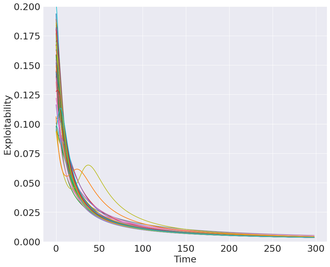
3p

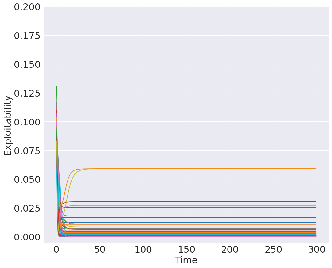
3r

Figure 1: Exploitability of 3p and 3r.

3r as an algorithm for the BSS problem.

In this section we evaluate the performance of 3r applied to the BSS problem. The global optimum OPT of the BSS problem for $\mathcal{H}_{2}\otimes\mathcal{H}_{2}$ and $\mathcal{H}_{2}\otimes\mathcal{H}_{3}$ systems can be obtained exactly by solving a semidefinite program.

Recall that the BSS problem corresponds to linear optimization over the set of separable states, which is in general hard to compute. In order to benchmark the performance of 3r we try to identify instances of the BSS problem that can be solved to optimality. For this, we rely on the Positive Partial Transpose (PPT) criterion for separability [60, 36]. Specifically, any density matrix $\rho$ describing the joint system $\mathcal{A}\otimes\mathcal{B}$ where $n=\dim\mathcal{A}$ and $m=\dim\mathcal{B}$, can be written as a block matrix

$$\rho=\begin{pmatrix}A_{11}&\ldots&A_{1n}\\ \vdots&&\vdots\\ A_{n1}&\ldots&A_{nn}\end{pmatrix},$$

where each block is an $m\times m$ matrix. The partial transpose of $\rho$ with respect to $\mathcal{B}$ is the matrix obtained from $\rho$ transposing each block $A_{ij}$, namely

$$\rho^{T_{\mathcal{B}}}=\begin{pmatrix}A_{11}^{T}&\ldots&A_{1n}^{T}\\ \vdots&&\vdots\\ A_{n1}^{T}&\ldots&A_{nn}^{T}\end{pmatrix},$$

and analogously we can also define the partial transpose of $\rho$ with respect to $\mathcal{A}$. The PPT criterion states that a necessary condition for $\rho$ to be separable is that the partial transpose $\rho^{T_{\mathcal{B}}}$ is positive semidefinite. Moreover, [36], based on previous work from [74] also show that the PPT criterion is necessary and sufficient when both $\mathcal{A}$ and $\mathcal{B}$ are qubit systems (i.e., $\mathcal{H}_{2}\otimes\mathcal{H}_{2}$) or when one of them is a qubit system and the other a qutrit (i.e., $\mathcal{H}_{2}\otimes\mathcal{H}_{3})$. Consequently, in these two regimes, the BSS problem corresponds to the following Semidefinite Program:

$$\max\{\langle R,\rho\rangle:\rho^{T_{B}}\succeq 0,\rho\succeq 0,\ \Tr(\rho)=1\},$$ (3u)

and consequently, it can be efficiently solved to optimality. Hence, we can benchmark the performance of 3r in the qubit vs. qubit or qubit vs. qutrit regimes by first computing the ground truth by solving the SDP (3u) which we then compare to the last iterate of 3r.

In each run of the experiments, we randomly generate a Hermitian positive definite matrix $R$ and standardize a uniform diagonal initialization (i.e. $\mathbb{1}_{\mathcal{H}}/n$) for 3r. We run 3r until convergence, which we detect by checking the moving average (window size $=5$) of the players’ utility and terminate the algorithm if the moving average stabilizes for several iterations. As a performance metric, we report the mean relative accuracy of 3r’s output compared to OPT across 100 runs. We also report the average number of iterations needed to find a fixed point/solution, along with the standard deviation of the accuracy across the 100 runs. All these results are summarized in Table 3. Figure 2 visualizes our results, and we also include a version of the experiment where the initializations for each player are random density matrices instead of uniform diagonal matrices. The solution to (3u) is computed using CVXPY [20, 1].

Table 3: Empirical performance of discrete dynamic 3r for the BSS problem.

Problem Dimensions	Runs	Accuracy		Average Iterations to Convergence
		Mean	Std. Dev.
$\mathcal{H}_{2}\otimes\mathcal{H}_{2}$	100	0.972	0.0410	14.12
$\mathcal{H}_{2}\otimes\mathcal{H}_{3}$	100	0.965	0.0351	16.97

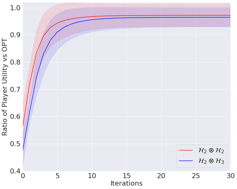
Random games, uniform initialization

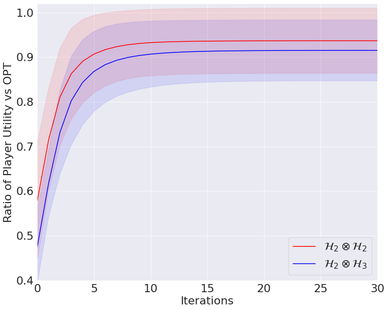
Random games, random initializations

Figure 2: Ratio of the utility attained using 3r vs OPT, averaged over 100 random BSS problem instances. Shaded region represents $\pm 1$ standard deviation from the mean, and each iteration represents alternating updates for $\rho$ and $\sigma$.

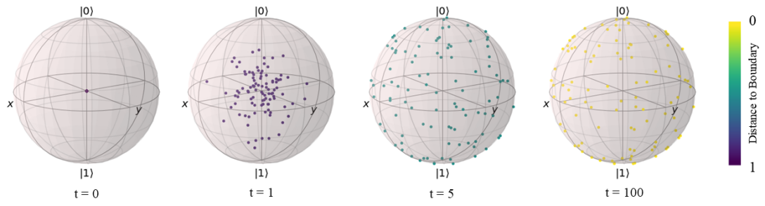
Figure 3: Trajectories going to the boundary of the Bloch-sphere in 100 random game instances with uniform density initializations. Points are color-coded based on distance to boundary, with yellow denoting points that are close the the boundary.

3r as an algorithm for biquadratic optimization.

In the quantum CIG setting, the players’ strategies are density matrices, which (via the SVD) correspond to distributions over rank-1 densities. Consequently, a quantum CIG can be viewed as the mixed extension of a common-interest game where players choose unit vectors and share a biquadratic utility. Our experiments suggest that when the players in a quantum CIG with game operator $R$ use the 3r, their states converge to rank-1 density matrices, an intriguing analogue of the convergence result for classical CIGs. Specifically, for a fixed, randomly generated game instance (i.e. a $4\times 4$ Hermitian $R\succ 0$), we run 3r on 100 randomly generated $\mathcal{H}_{2}\otimes\mathcal{H}_{2}$ games with uniform initialization for both players and visualize them on the Bloch sphere (Figure 3), which is a standard technique for visualizing $2\times 2$ density matrices and achieved using the QuTiP package [44].

For completeness, we now briefly describe the Bloch-sphere representation. The Pauli matrices are given by

$$\begin{gathered}{\sigma_{0}=\begin{pmatrix}1&0\\ 0&1\end{pmatrix}},\;\sigma_{1}=\begin{pmatrix}0&1\\ 1&0\end{pmatrix},\\ \sigma_{2}=\begin{pmatrix}0&-i\\ i&0\end{pmatrix},\sigma_{3}=\begin{pmatrix}1&0\\ 0&-1\end{pmatrix}.\end{gathered}$$

The (non-identity) Pauli matrices are Hermitian, their trace is equal to zero, they have $\pm 1$ eigenvalues, pairwise anti-commute and form an orthogonal basis of the $2\times 2$ complex matrices. Next we show that any $2\times 2$ density operator $\rho$ can be represented as a real 3-dimensional vector with Euclidean norm at most 1, where vectors with norm equal to 1 correspond to pure states. We visualize these 3-dimensional vectors as points on a sphere, known as the Bloch sphere. Specifically, we have that $\rho$ can be written as

$$\rho={1\over 2}(I_{2}+\sum_{i=1}^{3}a_{i}\sigma_{3}),\text{ where }\|a\|_{2}\leq 1,$$

and moreover, $\rho$ is pure iff $\|a\|_{2}=1$. To see this, we expand $\rho$ in the Pauli basis, i.e., $\rho=\sum_{i=0}^{3}a_{i}\sigma_{i},$ where $a_{i}={\Tr(\rho\sigma_{i})/\Tr(\sigma_{i}^{2})}.$ Recalling that $\sigma_{i}^{2}=I_{2}$ we finally get that

$$\rho={1\over 2}(I+\sum_{i=1}^{3}a_{i}\sigma_{3}),\text{ where }a_{i}=\Tr(\rho\sigma_{i}).$$

Lastly, note that all $a_{i}$’s are real (as the inner product of Hermitian matrices) and the eigenvalues of $\sum_{i=1}^{3}a_{i}\sigma_{3}$ are $\pm\|a\|$. Thus, for $\rho$ to be PSD we need that $\|a\|\leq 1$. Lastly, $\rho$ is pure iff $\Tr(\rho^{2})=1$, which is equivalent to $\|a\|_{2}=1$.

In addition to the specific game instance with random initializations in Figure 3, we also explore 3r for a fixed game instance. In particular, we run 3r on a fixed, randomly generated game with 100 randomly generated density initialization. The game generated is in $\mathcal{H}_{2}\otimes\mathcal{H}_{2}$. We then observe a similar phenomenon as before, with 3r generating trajectories that converge to the boundary of the Bloch sphere (Figure 4) for each initialization.

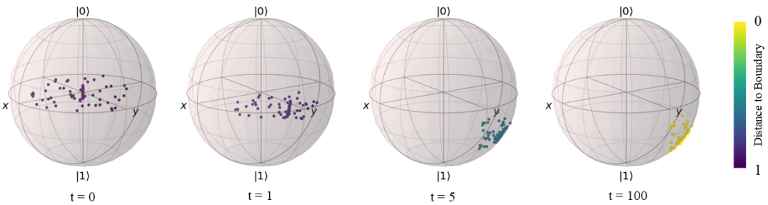
Figure 4: Trajectories going to the boundary of the Bloch sphere in a fixed game instance with 100 randomized density initializations. Points are color-coded based on distance to boundary, with yellow denoting points that are close the the boundary.

Since rank-1 densities in the quantum CIG correspond to unit vectors in the biquadratic optimization problem over the product of unit spheres $\max\{(x\otimes y)^{\dagger}R(x\otimes y):\|x\|_{2}=1,{\|y\|_{2}=1}\}$, this means that 3r can be interpreted as a learning algorithm for solving the biquadratic problem.

Large-scale experiments.

Finally, we present larger-scale experiments which show that our results for convergence to fixed points still holds in systems of larger dimensions.

Thus far we have focused on problems of dimension $\mathcal{H}_{2}\otimes\mathcal{H}_{2}$ and $\mathcal{H}_{2}\otimes\mathcal{H}_{3}$ since we can efficiently compute the optimal value. In order to test the efficacy of 3r for larger-scale problems, we run 3r in randomly generated problems of size $\mathcal{H}_{10}\otimes\mathcal{H}_{10}$ and $\mathcal{H}_{20}\otimes\mathcal{H}_{20}$. In Figure 5 we see that the dynamics converge to fixed points, like in the smaller scale experiments.

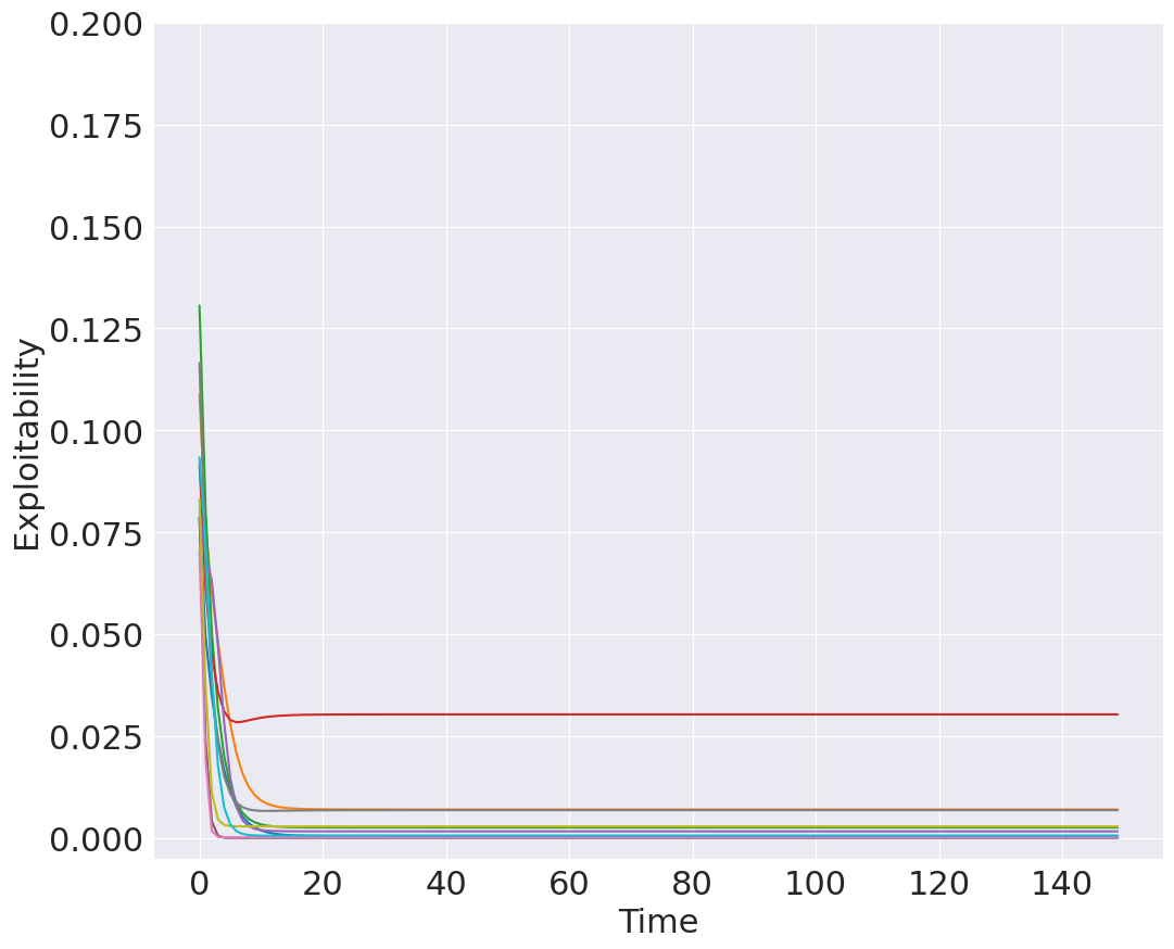
$\mathcal{H}_{10}\otimes\mathcal{H}_{10}$

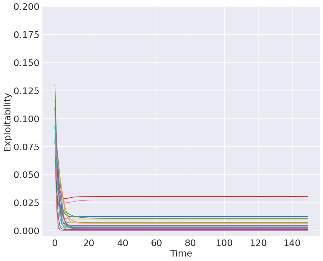
$\mathcal{H}_{20}\otimes\mathcal{H}_{20}$

Figure 5: Exploitability of 3r when applied to 10 randomly generated common-interest games.

Despite the low exploitability, it is not a guarantee that the dynamics have fully stabilized. Hence, for each run of the simulation, we additionally visualize the Frobenius norm between the dynamics at each timestep and the next iterate of the dynamics. Notice that in Figure 6, the log of the Frobenius norm generally decreases steadily over time, implying the dynamics stabilize and do not exhibit any oscillating behaviour.

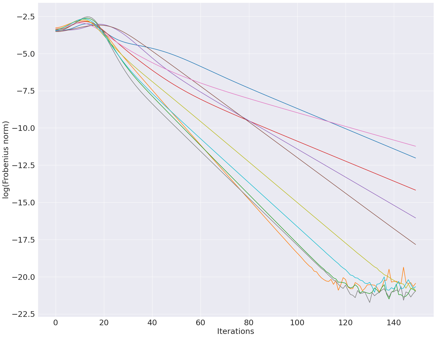
$\mathcal{H}_{10}\otimes\mathcal{H}_{10}$

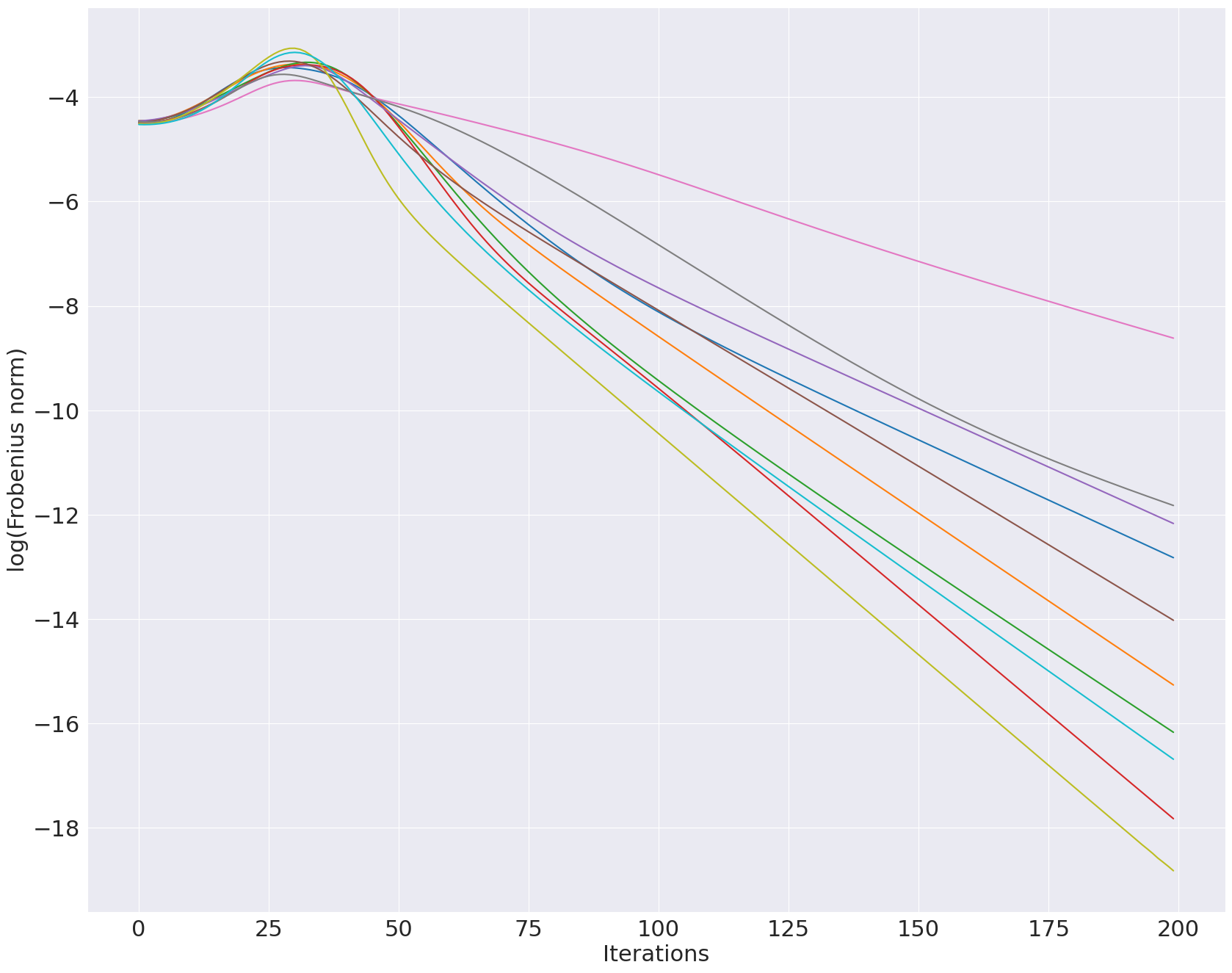
$\mathcal{H}_{20}\otimes\mathcal{H}_{20}$

Figure 6: Frobenius norm between 3r dynamic at each time step and the next iterate.

Table 4: Empirical performance of discrete dynamic lin-MMWU (stepsize $=0.9$) for the BSS problem.

Problem Dimensions	Runs	Accuracy		Average Iterations to Convergence
		Mean	Std. Dev.
$\mathcal{H}_{2}\otimes\mathcal{H}_{2}$	100	0.977	0.0343	29.76
$\mathcal{H}_{2}\otimes\mathcal{H}_{3}$	100	0.972	0.0324	35.69

Comparing lin-MMWU to 3r.

lin-MMWU is a more tunable version of 3r, and we are able to empirically show a difference in performance between these two algorithms. Figure 7 compares the exploitability of lin-MMWU with different stepsizes and 3r, showing that some runs clearly attain a lower exploitabiltiy when using lin-MMWU. Next, we compare the average case performance of each algorithm using the SDP benchmarking technique. The experimental setup is the same as before, and we set stepsize $\epsilon=0.9$. The performance of lin-MMWU is shown in Table 4.

Beyond benchmarking average case performance via SDPs, we are also interested in testing how much better the performance of lin-MMWU is compared to 3r. We consider the metrics of exploitability and utility. We performed 1000 runs of lin-MMWU and 3r and found that in $93.1\%$ of runs, lin-MMWU with stepsize $=0.9$ obtained lower exploitability than 3r, while in $99.6\%$ of runs lin-MMWU obtained higher utility than 3r. The average percentage decrease in exploitability is $36.3\%$, while the percentage improvement in utility is $0.635\%$. Thus, while the utility gain is not very high, empirically lin-MMWU still consistently finds less exploitable and higher utility fixed points than 3r. We note that the stepsize of $0.9$ is selected in order to balance performance and convergence at a reasonable rate.

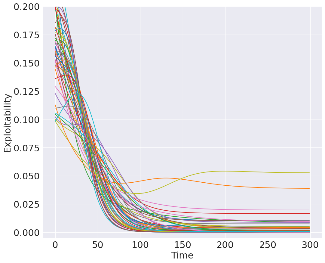
lin-MMWU ($\epsilon=0.1$)

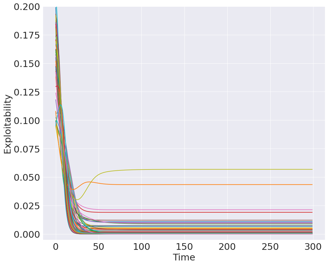
lin-MMWU ($\epsilon=0.5$)

3r

Figure 7: Comparing exploitability of lin-MMWU and 3r.

Improving empirical performance using perturbation.

Notice that in Figures 1 and 7, there are two game instances that perform poorly (i.e., high exploitability) for both discrete algorithms (3r and lin-MMWU). This indicates that the dynamics converge to a sub-optimal stationary point. In order to improve performance, we introduce the following modification of both algorithms: whenever a sub-optimal stationary point is reached, the players apply a random perturbation to their strategy and perform the subsequent update using this perturbed strategy. In principle, players may choose to perturb in the direction of their best response, but if the game matrix is unknown to players they can also perturb randomly, which suffices to drastically reduce exploitability (see Figure 8). We also note that while the fixed points converged to in these two game examples are entirely different after perturbation, they are still rank-1 density matrices. We provide further examples and explanation of the perturbation modification in Appendix LABEL:appsecs:additionalexperiments.

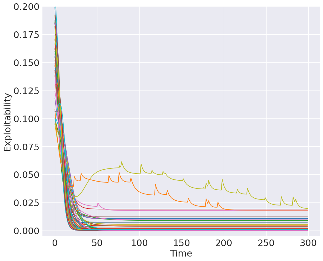
Random perturbation

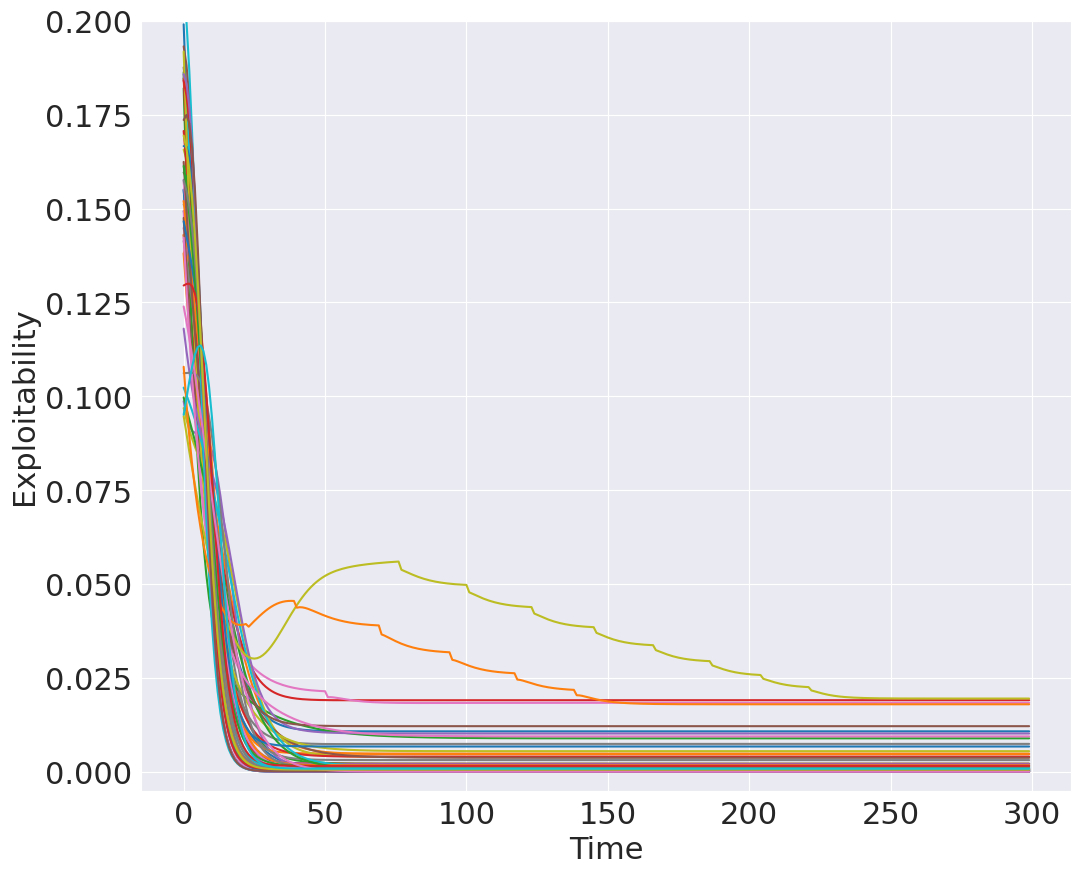
Best-response perturbation

Figure 8: Exploitability of lin-MMWU after perturbation.

6 Conclusion

This paper uses gamification to study the Best Separable State problem, and introduces several new algorithms that solve the problem approximately. In order to accomplish this, we introduce and study quantum common-interest games (CIGs) and establish and equivalence between the first-order stationary points of a BSS instance and the Nash equilibria of a corresponding quantum CIG. For learning in quantum CIGs we introduce non-commutative extensions of continuous and discrete dynamics used for learning in classical potential games, completing the picture of analogues of the classical replicator and multiplicative weight update learning dynamics (see Table 2), and study their convergence properties. Our work establishes deep connections between (online) optimization theory (i.e. multiplicative weights update), traditional as well as evolutionary game theory (i.e. replicator dynamics), and quantum randomness/entanglement (i.e. density matrices).

This work opens up several exciting new research directions, the first of which is to theoretically corroborate the experimental findings for convergence of 3p to Nash equilibria. Another intriguing open question is to what extent and under what conditions the 3r dynamics can be provably shown to converge to a rank-1 matrix for both players in quantum CIGs in analogy to aforementioned classical results [47, 32, 59]. More broadly, the ultimate goal of this line of research is to develop a general theory for learning in arbitrary quantum games. Developing such a framework would require new notions of equilibration and convergence in quantum games, echoing well-explored results for learning in classical games [6, 14, 24, 63].

Appendix A Properties of 3p

In this section we show that time derivative of the state $(\rho_{0},\sigma_{0})$ under the quantum replicator dynamics (3p) is always in the product of the tangent cones of $\rho_{0}\in D(\mathcal{A})$ and $\sigma_{0}\in D(\mathcal{B})$, i.e., it does not point outside of the state space. To do this we first recall the notion of the cone of feasible directions and the tangent cone:

Given a closed convex set $C$ in a Hilbert space and a point $x\in C$, the cone of feasible directions at $x$ is given by

$$\mathrm{dir}_{C}(x)=\{d:x+td\in C\text{ for some }t>0\}$$

and the tangent cone $\mathrm{T}_{C}(x)$ at $x$ (see, e.g, [61]) is given by the closure of the cone of feasible directions, i.e.,

$$\mathrm{T}_{C}(x)=\overline{\mathrm{dir}_{C}(x)}.$$

We shall characterize the tangent cones of points in the set of density matrices using the fact that the tangent cone is the polar to the normal cone. We first make the following observation characterizing the normal cones to the PSD cone:

Lemma A.1.

The normal cone to a matrix $X$ in the PSD cone, $N_{\mathrm{PSD}}(X)\equiv\{Z:\left\langle Z,Y-X\right\rangle\leq 0\;\forall\,Y\succeq 0\}$, is equal to the set $\{Z\preceq 0:\left\langle Z,X\right\rangle=0\}$.

Proof.

If $Z\preceq 0$ and $\left\langle Z,X\right\rangle=0$, then $\forall\,Y\succeq 0$ we have that $\left\langle Z,Y-X\right\rangle=\left\langle Z,Y\right\rangle-\left\langle Z,Y\right\rangle=\left\langle Z,X\right\rangle\leq 0$, so $Z\in N_{\mathrm{PSD}}(X)$.

On the other hand, if $Z\in N_{\mathrm{PSD}}(X)$ so that $\left\langle Z,Y-X\right\rangle\leq 0\;\forall\,Y\succeq 0$, then we can in particular consider the PSD matrix $Y:=X+vv^{\dagger}$ for any vector $v$. Then $v^{\dagger}Zv=\left\langle Z,vv^{\dagger}\right\rangle=\left\langle Z,Y-X\right\rangle\leq 0\;\forall\,v$, so we have that $Z\preceq 0$. It then follows that $\left\langle Z,X\right\rangle\leq 0$. However, taking $Y:=\frac{1}{2}X$ in the definition of the normal cone, we have that $\frac{1}{2}\left\langle Z,X\right\rangle=-\left\langle Z,-\frac{1}{2}X\right\rangle=-\left\langle Z,Y-X\right\rangle\geq 0$. Thus $\left\langle Z,X\right\rangle=0$. ∎

This gives us the following characterization of the tangent cones to the PSD cone:

Lemma A.2.

$\mathrm{T}_{D(\mathcal{A})}(\rho)=\{W:\tr(W)=0,\;u^{\dagger}Wu\geq 0\;\forall u\in\ker\rho\}$.

Proof.

Given a closed convex set $C$ and a point $x\in C$, the tangent cone at $x$ is the polar of the normal cone at $x$, i.e. $\mathrm{T}_{C}(x)=N_{C}(x)^{\circ}$ where the normal cone at $x$ is given by $N_{C}(x)\equiv\{z:\left\langle z,y-x\right\rangle\leq 0\;\forall y\in C\}$, and the polar of a set $S$ is given by $S^{\circ}=\{w:\left\langle w,z\right\rangle\leq 0\;\forall z\in S\}$ (see, e.g., [61]) .

For a Hermitian matrix $X$ in the PSD cone, we have from Lemma A.1 that the normal cone at $X$ is given by

$$N_{\mathrm{PSD}}(X)= \{Z:\left\langle Z,Y-X\right\rangle\leq 0\;\forall\,Y\succeq 0\}$$

$$= \{Z\preceq 0:\left\langle Z,X\right\rangle=0\},$$

and so the tangent cone at $X$ is given by

$$\mathrm{T}_{\mathrm{PSD}}(X)=N_{\mathrm{PSD}}(X)^{\circ}=\{W:u^{\dagger}Wu\geq 0\;\forall u\in\ker X\}.$$

Finally, we have that

$$\begin{split}&\mathrm{T}_{D(\mathcal{A})}(X)\\ =&\mathrm{T}_{\mathrm{PSD}}(X)\cap\mathrm{T}_{\tr=1}(X)\\ =&\{W:u^{\dagger}Wu\geq 0\;\forall u\in\ker X\}\cap(\tr=0)\\ =&\{W:\tr W=0,\;u^{\dagger}Wu\geq 0\;\forall u\in\ker X\}.\end{split}$$

∎

With this characterization of the tangent cone in hand, we are now ready to prove the theorem:

Theorem A.1.

At any point $(\rho,\sigma)\in D(\mathcal{A})\times D(\mathcal{B})$, the time derivatives $\dot{\rho}=\rho^{\nicefrac{{1}}{{2}}}\Big{[}\Phi(\sigma)-\left\langle\rho,\Phi(\sigma)\right\rangle\operatorname{\mathbb{1}}_{\mathcal{A}}\Big{]}\rho^{\nicefrac{{1}}{{2}}}$, $\dot{\sigma}=\sigma^{\nicefrac{{1}}{{2}}}\Big{[}\Phi^{\dagger}(\rho)-\left\langle\rho,\Phi(\sigma)\right\rangle\operatorname{\mathbb{1}}_{\mathcal{B}}\Big{]}\sigma^{\nicefrac{{1}}{{2}}}$ given by 3p lie in the tangent cones $\mathrm{T}_{D(\mathcal{A})}(\rho)$, $\mathrm{T}_{D(\mathcal{B})}(\sigma)$ respectively.

Proof.

Firstly, the time derivative $\dot{\rho}$ is traceless since

$$\tr(\rho^{\nicefrac{{1}}{{2}}}\Big{[}\Phi(\sigma)-\left\langle\rho,\Phi(\sigma)\right\rangle\operatorname{\mathbb{1}}_{\mathcal{A}}\Big{]}\rho^{\nicefrac{{1}}{{2}}})$$

$$=$$

References

- [1] A. Agrawal, R. Verschueren, S. Diamond, and S. Boyd. A rewriting system for convex optimization problems. Journal of Control and Decision, 5(1):42–60, 2018.
- [2] Z. Allen-Zhu, Z. Liao, and L. Orecchia. Spectral sparsification and regret minimization beyond matrix multiplicative updates. In Proceedings of the forty-seventh annual ACM symposium on Theory of computing, pages 237–245, 2015.
- [3] S. Arora, E. Hazan, and S. Kale. Fast algorithms for approximate semidefinite programming using the multiplicative weights update method. In 46th Annual IEEE Symposium on Foundations of Computer Science (FOCS’05), pages 339–348. IEEE, 2005.
- [4] S. Arora, E. Hazan, and S. Kale. The multiplicative weights update method: a meta-algorithm and applications. Theory of computing, 8(1):121–164, 2012.
- [5] S. Arora and S. Kale. A combinatorial, primal-dual approach to semidefinite programs. In Proceedings of the thirty-ninth annual ACM symposium on Theory of computing, pages 227–236, 2007.
- [6] J. P. Bailey and G. Piliouras. Multiplicative weights update in zero-sum games. In ACM Conference on Economics and Computation, 2018.
- [7] N. Bard, J. N. Foerster, S. Chandar, N. Burch, M. Lanctot, H. F. Song, E. Parisotto, V. Dumoulin, S. Moitra, E. Hughes, et al. The hanabi challenge: A new frontier for ai research. Artificial Intelligence, 280:103216, 2020.
- [8] L. E. Baum and J. A. Eagon. An inequality with applications to statistical estimation for probabilistic functions of markov processes and to a model for ecology. Bulletin of the American Mathematical Society, 73(3):360–363, 1967.
- [9] M. Berta, F. Borderi, O. Fawzi, and V. B. Scholz. Semidefinite programming hierarchies for constrained bilinear optimization. Mathematical Programming, 194(1):781–829, 2022.
- [10] M. Berta, O. Fawzi, and V. B. Scholz. Quantum bilinear optimization. SIAM Journal on Optimization, 26(3):1529–1564, 2016.
- [11] R. Bhatia. Positive definite matrices. Princeton university press, 2009.
- [12] I. M. Bomze. Lotka-Volterra equation and replicator dynamics: a two-dimensional classification. Biological cybernetics, 48(3):201–211, 1983.
- [13] J. Bostanci and J. Watrous. Quantum game theory and the complexity of approximating quantum nash equilibria. Quantum, 6:882, 2022.
- [14] N. Cesa-Bianchi and G. Lugosi. Prediction, learning, and games. Cambridge university press, 2006.
- [15] G. Chiribella, G. M. D’Ariano, and P. Perinotti. Theoretical framework for quantum networks. Physical Review A, 80(2):022339, 2009.
- [16] A. Dafoe, Y. Bachrach, G. Hadfield, E. Horvitz, K. Larson, and T. Graepel. Cooperative ai: machines must learn to find common ground. Nature, 2021.
- [17] A. Dafoe, E. Hughes, Y. Bachrach, T. Collins, K. R. McKee, J. Z. Leibo, K. Larson, and T. Graepel. Open problems in cooperative ai. arXiv preprint arXiv:2012.08630, 2020.
- [18] C. Daskalakis, S. Skoulakis, and M. Zampetakis. The complexity of constrained min-max optimization. In Proceedings of the 53rd Annual ACM SIGACT Symposium on Theory of Computing, pages 1466–1478, 2021.
- [19] D. Della Penda, A. Abrardo, M. Moretti, and M. Johansson. Potential games for subcarrier allocation in multi-cell networks with d2d communications. In 2016 IEEE International Conference on Communications (ICC), pages 1–6. IEEE, 2016.
- [20] S. Diamond and S. Boyd. CVXPY: A Python-embedded modeling language for convex optimization. Journal of Machine Learning Research, 17(83):1–5, 2016.
- [21] A. C. Doherty, P. A. Parrilo, and F. M. Spedalieri. Complete family of separability criteria. Physical Review A, 69(2):022308, 2004.
- [22] J. Eisert, M. Wilkens, and M. Lewenstein. Quantum games and quantum strategies. Physical Review Letters, 83(15):3077, 1999.
- [23] Y. Freund and R. E. Schapire. A decision-theoretic generalization of on-line learning and an application to boosting. Journal of computer and system sciences, 55(1):119–139, 1997.
- [24] D. Fudenberg, F. Drew, D. K. Levine, and D. K. Levine. The theory of learning in games, volume 2. MIT press, 1998.
- [25] D. Fudenberg and J. Tirole. Game theory. MIT press, 1991.
- [26] I. Gemp, B. McWilliams, C. Vernade, and T. Graepel. Eigengame: PCA as a nash equilibrium. arXiv preprint arXiv:2010.00554, 2020.
- [27] S. Gharibian. Strong NP-hardness of the quantum separability problem. arXiv preprint arXiv:0810.4507, 2008.
- [28] M. Grötschel, L. Lovász, and A. Schrijver. Geometric algorithms and combinatorial optimization, volume 2. Springer Science & Business Media, 2012.
- [29] L. Gurvits. Classical deterministic complexity of Edmonds’ problem and quantum entanglement. In Proceedings of the thirty-fifth annual ACM symposium on Theory of computing, pages 10–19, 2003.
- [30] G. Gutoski and J. Watrous. Toward a general theory of quantum games. In Proceedings of the thirty-ninth annual ACM symposium on Theory of computing, pages 565–574, 2007.
- [31] Q. He, G. Cui, X. Zhang, F. Chen, S. Deng, H. Jin, Y. Li, and Y. Yang. A game-theoretical approach for user allocation in edge computing environment. IEEE Transactions on Parallel and Distributed Systems, 31(3):515–529, 2019.
- [32] A. Heliou, J. Cohen, and P. Mertikopoulos. Learning with bandit feedback in potential games. Advances in Neural Information Processing Systems, 30, 2017.
- [33] J. Hofbauer and W. H. Sandholm. On the global convergence of stochastic fictitious play. Econometrica, 70(6):2265–2294, 2002.
- [34] J. Hofbauer and K. Sigmund. Evolutionary game dynamics. Bulletin of the American mathematical society, 40(4):479–519, 2003.
- [35] J. Hofbauer, K. Sigmund, et al. Evolutionary games and population dynamics. Cambridge university press, 1998.
- [36] M. Horodecki, P. Horodecki, and R. Horodecki. On the necessary and sufficient conditions for separability of mixed quantum states. Phys. Lett. A, 223(11), 1996.
- [37] S. Huber, R. König, and M. Tomamichel. Jointly constrained semidefinite bilinear programming with an application to Dobrushin curves. IEEE Transactions on Information Theory, 66(5):2934–2950, 2019.
- [38] C. Ickstadt, T. Theobald, and E. Tsigaridas. Semidefinite games. arXiv preprint arXiv:2202.12035, 2022.
- [39] L. M. Ioannou. Computational complexity of the quantum separability problem. arXiv preprint quant-ph/0603199, 2006.
- [40] R. Jain, Z. Ji, S. Upadhyay, and J. Watrous. QIP=PSPACE. Journal of the ACM (JACM), 58(6):1–27, 2011.
- [41] R. Jain, G. Piliouras, and R. Sim. Matrix multiplicative weights updates in quantum zero-sum games: Conservation laws & recurrence. arXiv preprint arXiv:2211.01681, 2022.
- [42] R. Jain and J. Watrous. Parallel approximation of non-interactive zero-sum quantum games. In 2009 24th Annual IEEE Conference on Computational Complexity, pages 243–253. IEEE, 2009.
- [43] M. Johanson, K. Waugh, M. Bowling, and M. Zinkevich. Accelerating best response calculation in large extensive games. In Twenty-second international joint conference on artificial intelligence, 2011.
- [44] J. R. Johansson, P. D. Nation, and F. Nori. QuTiP: An open-source python framework for the dynamics of open quantum systems. Computer Physics Communications, 183(8):1760–1772, 2012.
- [45] S. Kale. Efficient algorithms using the multiplicative weights update method. Princeton University, 2007.
- [46] H. Kitano, M. Asada, Y. Kuniyoshi, I. Noda, E. Osawa, and H. Matsubara. Robocup: A challenge problem for ai. AI magazine, 18(1):73–73, 1997.
- [47] R. Kleinberg, G. Piliouras, and É. Tardos. Multiplicative updates outperform generic no-regret learning in congestion games. In Proceedings of the forty-first annual ACM symposium on Theory of computing, pages 533–542, 2009.
- [48] Q. D. Lã, Y. H. Chew, and B.-H. Soong. Potential games. In Potential Game Theory, pages 23–69. Springer, 2016.
- [49] V. Losert and E. Akin. Dynamics of games and genes: Discrete versus continuous time. Journal of Mathematical Biology, 17(2):241–251, 1983.
- [50] J. R. Marden, G. Arslan, and J. S. Shamma. Cooperative control and potential games. IEEE Transactions on Systems, Man, and Cybernetics, Part B (Cybernetics), 39(6):1393–1407, 2009.
- [51] P. Mertikopoulos and W. H. Sandholm. Learning in games via reinforcement and regularization. Mathematics of Operations Research, 41(4):1297–1324, 2016.
- [52] P. Mertikopoulos and W. H. Sandholm. Riemannian game dynamics. Journal of Economic Theory, 177:315–364, 2018.
- [53] D. A. Meyer. Quantum strategies. Physical Review Letters, 82(5):1052, 1999.
- [54] D. Monderer and L. S. Shapley. Potential games. Games and economic behavior, 14(1):124–143, 1996.
- [55] M. Moravčík, M. Schmid, N. Burch, V. Lisỳ, D. Morrill, N. Bard, T. Davis, K. Waugh, M. Johanson, and M. Bowling. Deepstack: Expert-level artificial intelligence in heads-up no-limit poker. Science, 356(6337):508–513, 2017.
- [56] A. S. Nemirovskij and D. B. Yudin. Problem complexity and method efficiency in optimization. 1983.
- [57] L. Orecchia, S. Sachdeva, and N. K. Vishnoi. Approximating the exponential, the Lanczos method and an O(m)-time spectral algorithm for balanced separator. In Proceedings of the forty-fourth annual ACM symposium on Theory of computing, pages 1141–1160, 2012.
- [58] G. Palaiopanos, I. Panageas, and G. Piliouras. Multiplicative weights update with constant step-size in congestion games: Convergence, limit cycles and chaos. Advances in Neural Information Processing Systems, 30, 2017.
- [59] I. Panageas, G. Piliouras, and X. Wang. Multiplicative weights updates as a distributed constrained optimization algorithm: Convergence to second-order stationary points almost always. In International Conference on Machine Learning, pages 4961–4969. PMLR, 2019.
- [60] A. Peres. Separability criterion for density matrices. Physical Review Letters, 77(8):1413, 1996.
- [61] R. T. Rockafellar. Clarke’s tangent cones and the boundaries of closed sets in . Nonlinear Analysis: theory, methods and applications, 3:145–154, 1979.
- [62] R. W. Rosenthal. A class of games possessing pure-strategy nash equilibria. International Journal of Game Theory, 2(1):65–67, 1973.
- [63] T. Roughgarden. Algorithmic game theory. Communications of the ACM, 53(7):78–86, 2010.
- [64] W. Rudin. Real and complex analysis (McGraw-Hill international editions: Mathematics series). 1987.
- [65] W. H. Sandholm. Population games and evolutionary dynamics. MIT press, 2010.
- [66] S. Shahshahani. A new mathematical framework for the study of linkage and selection. American Mathematical Soc., 1979.
- [67] D. Silver, A. Huang, C. J. Maddison, A. Guez, L. Sifre, G. Van Den Driessche, J. Schrittwieser, I. Antonoglou, V. Panneershelvam, M. Lanctot, et al. Mastering the game of go with deep neural networks and tree search. nature, 529(7587):484–489, 2016.
- [68] S. H. Singh. A Non-Negative Matrix Factorization game. arXiv preprint arXiv:2104.05069, 2021.
- [69] P. Stone, G. Kaminka, S. Kraus, and J. Rosenschein. Ad hoc autonomous agent teams: Collaboration without pre-coordination. In Proceedings of the AAAI Conference on Artificial Intelligence, volume 24, pages 1504–1509, 2010.
- [70] P. D. Taylor and L. B. Jonker. Evolutionary stable strategies and game dynamics. Mathematical biosciences, 40(1-2):145–156, 1978.
- [71] K. Tsuda, G. Rätsch, and M. K. Warmuth. Matrix exponentiated gradient updates for on-line learning and Bregman projection. Journal of Machine Learning Research, 6(Jun):995–1018, 2005.
- [72] J. W. Weibull. Evolutionary game theory. MIT press, 1997.
- [73] A. Wibisono, A. C. Wilson, and M. I. Jordan. A variational perspective on accelerated methods in optimization. proceedings of the National Academy of Sciences, 113(47):E7351–E7358, 2016.
- [74] S. L. Woronowicz. Positive maps of low dimensional matrix algebras. Reports on Mathematical Physics, 10(2):165–183, 1976.
- [75] J. Zeng, Q. Wang, J. Liu, J. Chen, and H. Chen. A potential game approach to distributed operational optimization for microgrid energy management with renewable energy and demand response. IEEE Transactions on Industrial Electronics, 66(6):4479–4489, 2018.
- [76] S. Zhang. Quantum strategic game theory. In Proceedings of the 3rd Innovations in Theoretical Computer Science Conference, pages 39–59, 2012.