Optical communication-based identification for multi-UAV systems: theory and practice

Abstract

Mutual relative localization and identification is an important feature for the stabilization and navigation of multi- Unmanned Aerial Vehicle (UAV) systems. Camera-based communications technology, also referred to as Optical Camera Communications (OCC) in the literature, is a novel approach that could bring a valuable solution to such a complex task. In such system, the UAVs are equipped with LEDs that act as beacons and with cameras allowing them to locate the LEDs of other UAVs. Specific blinking sequences are assigned to the LEDs of each of the UAVs in order to uniquely identify them. This camera-based relative localization and identification system is immune to Radio Frequency (RF) electromagnetic interference and operates in Global Navigation Satellite (GNSS) denied environments. In addition, since many UAVs are already equipped with cameras, the implementation of this system is inexpensive. In this article, we study in detail the capacity of this system and its limitations. Furthermore, we show how to construct blinking sequences for UAV LEDs in order to improve system performance. Finally, experimental results are presented to corroborate the analytical derivations.

I Introduction

Mutual relative localization and identification is an important feature in multi-UAV systems that is useful for motion coordination and cooperative task planning. While the relative localization is important for close cooperative flying and mutual collision avoidance, the identification of neighboring vehicles of the team, which is the prime focus of this paper, is crucial for all high-level planning mechanisms. This feature can be implemented by means of either RF electromagnetic signals or by using vision-based techniques, or through a combination of both. For instance, in [1, 2], RTK-GNSS is used for UAV localization. In [3], Ultra Wide Band (UWB) ranging is used to determine the distance between UAVs. In [4], a motion capture system integrated with infrared cameras is used. A set of markers reflecting emitted infrared light is attached to the UAV and the motion capture system estimates and sends its position estimate to the UAV via an RF link. Such localization techniques, based on RF, are vulnerable to electromagnetic interference and may fail in providing mutual identification in multi-robot systems. On the other hand, vision-based techniques are immune to electromagnetic interference and can be used to provide relative localization and identification in multi-robot systems.

Vision-based localization and identification systems can be divided into passive and active systems. Passive systems use optical markers that do not emit light, whereas active systems use optical markers which emit light. In [5], the authors present a passive system where specific marker patterns are assigned to each robot. The same passive system was used in [6] for localization and identification of UAVs in an outdoor scenario. One of the main disadvantages of passive systems is their sensitivity to ambient light. Thus, they do not work well in poorly illuminated environments. These problems are solved by using active vision-based localization and identification systems. In such techniques, the active markers of UAVs are generally implemented with energy-efficient LED light sources.

In [7], the authors equipped a UAV with infrared LEDs and used a CMOS camera to perform localization in an indoor scenario. Different blinking frequencies were assigned to each LED in order to differentiate them. Square blinking signals in the range of 1-2kHz were chosen. Their frequencies were set in such a way that no two signals shared common harmonics, so as to avoid ambiguities in their discrimination. In [8, 9, 10, 11], our research group presented the UltraViolet Direction And Ranging (UVDAR) system for UAVs, see Fig. 1 and Fig. 2. In this system, UAVs are equipped with Ultraviolet (UV) LEDs as markers and cameras coupled with optical filters that attenuate most visible light, but still allow UV light to pass. Similar to the previously mentioned method, the optical signals emitted by the LEDs were square signals of different frequencies. The commonplace use of square signals at different frequencies is a straightforward way to discriminate between the different blinking patterns emitted by all LEDs. However, this is an inefficient technique, as will be demonstrated further in this article.

In the field of communications, the Optical Camera Communications (OCC) system, in which the transmitter is a LED and the receiver is a camera [12, 13], has been used for car-to-car communications and car-to-infrastructure communications [14, 15, 16, 17, 18]. Despite the fact that the purpose of the OCC system is to exchange information, the theory developed for these types of systems [19, 20, 21] can be used to improve the active vision-based localization and identification systems for UAVs.

This article focuses on the mutual identification capacity of a vision-based active system; the relative localization issue is beyond its scope. We investigate mutual identification using the UVDAR system, mentioned above.

Our research group developed the UVDAR system as a proof-of-concept placeholder for different relative localization and identification systems. In addition, the UVDAR system has been used for a variety of experimental applications where it is essential that the localization and the identification of UAVs is implemented independent of any infrastructure. These applications include swarming or flocking both in open spaces [11] and in obstacle-filled environments [22], visual communication [23], directed leader-follower behavior [24], hostile agent avoidance and shepherding [25], landing on moving platforms [26], automated building of visual training datasets for machine learning [27], and formation flights.

Figure 1: A pair of DJI F450-based UAV platforms equipped with the UVDAR system. Note the ultraviolet LEDs on the sides of the UAV body.

In this paper, we propose an approach inspired by the theory developed for OCC systems. This theory was developed for vehicular communications, but has never been used for localization or identification of UAVs. Since the requirements and operational conditions of the two problems differ, the theory developed for OCC must be adjusted and expanded before it can be applied to the problem of UAV.

The main contributions of this article are as follows:

• Blinking sequence generation method: a theoretical framework was developed to design sets of blinking sequences for the LEDs of groups of UAV. These sequence sets are optimized to discriminate between as many sequences as possible in the shortest amount of time. This will enable large groups of UAVs to perform mutual identification in the shortest time possible.

• Theoretical analysis of UVDAR: we performed an analytical analysis to derive the probability of misdetection of the blinking sequences. We derived analytical formulas to determine the number of different blinking sequences that can be detected as a function of their length. We further calculated the limit of the sequence length as a function of the UAVs clock signals. This can be used to calculate the total number of UAVs that can be identified by this system, depending on the quality of their clock signals.

• Experimental validation: we implemented a prototype of the proposed vision-based mutual identification system for UAVs and tested it outdoors.

The article is organized as follows. In section II, we describe the system model. This includes the models for the UAV clock signal, for the optical identification system, and for the optical transmission channel. In section III, we derive the optical Signal-to-Noise Ratio (SNR). In section IV, we formalize the problem of the visual identification system for UAVs. In section V, we describe the theoretical framework for the construction of the LEDs’ blinking sequences using the Non-Return-to-Zero (NRZ) optical modulation (a popular optical modulation scheme). In section VI, we show how the use of the Manchester optical modulation (another popular optical modulation scheme), instead of the NRZ, changes the properties of the identification system. In section VII, we study the effects of the UAVs clock on the performance of the identification system. Section VIII describes the experiments performed. Conclusions are provided in section IX.

II System Model

We consider a group of UAVs composed of $J$ members. Each UAV is equipped with the UVDAR system, see Fig. 2 and Fig. 3. The system is composed mainly of three modules (as shown in Fig. 3): the optical transmitter, the optical receiver, and the clock signal generator. In this section, we will discuss the three modules in detail, as well as the optical channel model, which describes the relationship between the emitted optical signals and the received optical signals.

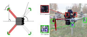
Figure 2: UAV equipped with the UVDAR system.

Figure 3: UVDAR block diagram of the $j$th UAV

II-A Clock signal

The clock signal’s falling (or rising) edges indicate the instants when the receiver’s camera shoots, and when the transmitter’s LEDs can change state. An ideal clock signal should be stable and the interval between falling (or rising) edges should always remain constant. Furthermore, the clock signal frequency of the different UAVs of the group should be exactly the same. Unfortunately, due to impairments, the clock signals are not perfectly stable. Even if all nominal frequencies of all clocks are the same, their true frequencies will differ slightly. These impairments and their effects on similar systems have been documented in the literature. For instance, in [28, 29], it was observed that the measured interframe interval of certain cameras is time-variant. In [12], it was noted in the context of smartphone cameras, that the nominal frame rate, fixed by software, differs from the true frame rate and varies depending on the phone.

These irregularities on the clock signal limit the capacity of the optical identification system studied in this article as it will be demonstrated in section VII. First, let us describe the model of the $j$th UAV clock signal, denoted by $c_{j}(t)$. Without loss of generality, we consider that the optical transmitter and receiver are controlled by the falling edges of $c_{j}(t)$. Based on the mathematical models for clock signals described in [30, 31], we model the $k$th falling edge instant of $c_{j}(t)$ as:

$$t_{j,k}=T_{j}+n_{j,k}+t_{j,k-1},\quad\quad k=1,2,$$ (1)

where $t_{j,0}$ is the instant when the system of the $j$th UAV is turned on; $t_{j,k}$ with $k\geq 1$ is the instant of the $k$th falling edge instant of $c_{j}(t)$; $T_{j}>0$ is the true clock signal period of $c_{j}(t)$ and is modelled as a random variable with mean $\mathbb{E}[T_{j}]=T$, with $T$ being the nominal period of the clock signal, and variance $\mathrm{var}[T_{j}]=\sigma^{2}_{T}$. Due to the fabrication process uncertainties, different clocks will have slightly different oscillation frequencies, even if their nominal frequencies are the same. Thus, we consider that the set $\{T_{j}\}_{j=1}^{J}$ is composed of $J$ statistically independent and identically distributed random variables. $n_{j,k}$ accounts for the frequency instability of the clock signal and is modelled as a white noise process.

II-B Optical Transmitter

Fig. 4 depicts the block diagram of the optical transmitter for the quadrotor shown in Fig. 2. The optical transmitter is divided into $M$ parallel branches. In this particular case, we select $M=4$, i.e., one transmitter branch per UAV arm in Fig. 2. Note that it is possible to have optical transmitters with more branches [8, 10], but a discussion on such configurations is beyond the scope of this article. The optical transmitter modules are:

• Binary stream generator $m$: it takes as inputs the clock signal $c_{j}^{d}(t)$ and a binary matrix $\mathbf{S}_{j}$ of size $M\times L$, which contains $M$ binary sequences of length $L$. The $m$th binary stream generator produces the discrete-time stream $s_{j,m}$ composed of a continuously repeated concatenation of the binary sequence contained in the $m$th row of the matrix $\mathbf{S}_{j}$; $s_{j,m}[k]\in\{0,1\}$ denotes the $k$th bit in the binary stream $s_{j,m}$. All the binary sequences used by the UAVs in the group are stored in a dictionary matrix $\mathbf{D}$; each row of the matrix $\mathbf{D}$ is a different binary sequence, and its identification number is the row number in which it is stored. The dictionary $\mathbf{D}$ is shared by all the UAVs in the group (see Fig. 5). Finally, the identification number embedded in the stream $s_{j,m}$ is the same as the identification number of the binary sequence used to generate it.

• Encoder and Modulator (Enc./Mod.): the encoder codifies the binary discrete-time stream $s_{j,m}$ with a line code, such as NRZ or Manchester [32]. The modulator modulates the encoded signal with On-Off Keying (OOK) [33] to produce the continuous-time electrical signal $u_{j,m}(t)\in\left\{0,1\right\}$.

• Frequency divider: it divides the clock signal frequency by a division factor $d_{f}$. The modulator and the encoder are both driven directly with the clock signal $c_{j}(t)$. However, the binary stream generator is driven by $c_{j}^{d}(t)$. If the Manchester code is used, then each bit consists of two minibits and the frequency of $c_{j}^{d}(t)$ must be half the frequency of $c_{j}(t)$, i.e., we need $d_{f}=2$. Alternatively, if the NRZ code is used, then each bit consists of only one minibit and thus the frequency of $c_{j}^{d}(t)$ must be equal to the frequency of $c_{j}(t)$, i.e. $d_{f}=1$.

• Analog frontend: this transforms the binary electrical signal $u_{j,m}(t)$ into the optical signal $v_{j,m}(t)=Pu_{j,m}(t)$, which represents the emitted optical power. Each frontend has two LEDs that emit the same optical signal with a wavelength of 400 nm, which falls into the UV spectrum. Both LEDs are mounted in orthogonal directions (see Fig. 2) to increase the angular range of visibility of the optical signal $v_{j,m}(t)$.

Figure 4: Optical transmitter architecture for the $j$th UAV.

II-C Optical Receiver

Figure 5: Optical receiver architecture for the $j$th UAV.

The optical receiver of the $j$th UAV follows the architecture shown in Fig. 5 and is composed of the following modules:

• Camera: a grey scale camera is mounted on the UAV as shown in Fig. 2. The camera is coupled with an optical filter that allows UV light to pass and filters-out most visible light, see [34]. The optical filter attenuates most of the background light and facilitates the detection of the UV light emitted by the other UAVs, see Fig. 6. The camera shoots at every falling edge of the clock signal $c_{j}(t)$ with an exposure time $\tau_{e}$. The $k$th frame captured is denoted as $\mathbf{F}_{j}[k]$. We denote the pixel of the $m$th row and $n$th column as $\left[\mathbf{F}_{j}[k]\right]_{m,n}$.

  

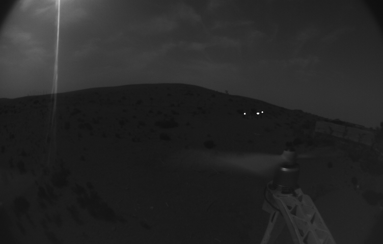
  Figure 6: Grey scale image produced by a UV camera used in the UVDAR system onboard a UAV. The three bright spots in the image are active UV LED markers on another UAV flying past. Note that despite the fact that this image was actually captured in extremely bright mid-day conditions in desert dunes near Abu Dhabi, there is a high contrast between the background and the markers.

• Image Processing: this module must detect the bright spots potentially generated by the UV LEDs from the other UAVs in the group, track their motion on the screen, and then extract the optical signal from their blinking patterns. To do this, the frame $\mathbf{F}_{j}[k]$ is first binarized with the threshold $\eta_{b}$ to produce $\bar{\mathbf{F}}_{j}[k]$. This simplifies the distinction between the background and bright spots potentially generated by UV LEDs, see Fig. 6. When a new bright spot is detected in $\bar{\mathbf{F}}_{j}[k]$, a serialized service number $n_{s}$ is assigned and the following operations take place simultaneously: i) the coordinates of the central pixel of the $n_{s}$th bright spot is estimated $\hat{\mathbf{p}}_{j,n_{s}}[k]$, and its motion on screen begins to be tracked; ii) the pixel with coordinates $\hat{\mathbf{p}}_{j,n_{s}}[k]$ is read in $\bar{\mathbf{F}}_{j}[k]$, and the values are stored as a binary time series $y_{j,n_{s}}[k]$. The instant when the time series associated to the $n_{s}$ bright spot is created is denoted as its birth time $t_{b,j,n_{s}}$; iii) a classifier instance is created to process the time series $y_{j,n_{s}}$.

  As long as the $n_{s}$th bright spot is successfully tracked, the associated time series $y_{j,n_{s}}$ remains alive. However, once the tracking fails, the time series $y_{j,n_{s}}$ dies and the classifier instance dedicated for processing it is destroyed. We denote this instant as the death time $t_{d,j,n_{s}}$ of time series $y_{j,n_{s}}$. Possible reasons for tracking failure may include LED occlusions, fast movements of the bright spot on the camera frame, or LED blinking patterns with long times off.

• Classifier. Each classifier takes as input the dictionary $\mathbf{D}$ described in section II-B and the last $L$ bits received in the binary stream $y_{j,n_{s}}$. The classifier output is the time-series $z_{j,n_{s}}[k]$ which is then fed into the upper modules, see Fig. 3. The first objective of the classifier is to determine if $\{y_{j,n_{s}}[m]\}_{m=k-L+1}^{k}$ was generated with a binary sequence contained in the dictionary $\mathbf{D}$. This allows for discarding bright spots generated by sources other than the UAVs, as can be the case of random dynamic reflections. As will be seen later in appendix B, this is done by calculating the correlation of $\{y_{j,n_{s}}[m]\}_{m=k-L+1}^{k}$ with the sequences contained into the dictionary $\mathbf{D}$, and then comparing it with a detection threshold $\eta_{d}$. If the classifier decides that $\{y_{j,n_{s}}[m]\}_{m=k-L+1}^{k}$ was not generated by a binary sequence contained in the dictionary $\mathbf{D}$, then it produces $z_{j,n_{s}}[k]=-1$. In the contrary case, the classifier estimates the identification number of the binary stream $y_{j,n_{s}}$; $z_{j,n_{s}}[k]$ takes on this number.

II-D Optical channel model

In this subsection, we describe the optical channel from different optical transmitters to the $j$th UAV camera. The value of the $\bar{\mathbf{F}}_{j}[k]$ pixels coinciding with the centers of the bright spots generated by the UV LEDs appearing in the $j$th UAV camera Field of View (FoV), including Line of Sight (LoS), can be modelled as follows:

$$\mathbf{y}_{j}[k]=\mathbf{1}_{+}(\mathbf{x}_{j}[k]-\eta_{b}),$$ (2)

$$\mathbf{x}_{j}[k]=\min\left(\max\left(\boldsymbol{\omega}_{j}[k],\mathbf{0}\right),{\bar{\boldsymbol{\omega}}}\right)+\mathbf{n}_{j,2,th}[k],$$ (3)

$$\boldsymbol{\omega}_{j}[k]=\int_{t_{j,k}}^{t_{j,k}+\tau_{e}}\mathbf{w}_{j}(t)\mathrm{d}t,$$ (4)

$$\mathbf{w}_{j}(t)=\mathbf{H}_{j}(t)\mathbf{v}_{j}(t)+\mathbf{d}_{j,n}(t)+\mathbf{n}_{j,sh}(t)+\mathbf{n}_{j,1,th}(t),$$ (5)

where $\mathbf{v}_{j}(t)$ is a column vector with $(J-1)2M$ entries containing all optical power emitted by the $2M$ UV LEDs of all of the UAVs in the group, excluding the $j$th UAV. In (5), $\mathbf{w}_{j}(t)$ is the instantaneous electrical signal generated at the pixels of interest before considering the exposition process, $\mathbf{H}_{j}(t)$ is the optical channel gain, $\mathbf{d}_{j,n}(t)$ is the dc level generated by the background illumination [30], $\mathbf{n}_{j,1,th}(t)$ is the thermal noise generated in the circuitry before the exposition [30]; and $\mathbf{n}_{j,sh}(t)$ is the shot noise [35, 36]. The entries of $\mathbf{n}_{j,1,th}(t)$ are statistically independent zero-mean white Gaussian noise processes with constant variance $\sigma_{th,1}^{2}$. The shot noise at a given pixel is modelled as Gaussian random process with a variance proportional to the incident power [35]. The shot noise variables generated at different pixels are statistically independent. Thus, the shot noise vector $\mathbf{n}_{j,sh}(t)$ is modeled as a zero-mean Gaussian vector with covariance matrix $\alpha\mathrm{diag}(\mathbf{H}_{j}(t)\mathbf{v}_{j}(t)+\mathbf{d}_{j,n}(t))$, where $\alpha$ is a proportionality constant depending on the particular hardware implementation [35, 36]. In Eq. (4), $\boldsymbol{\omega}_{j}[k]$ represents the values of the pixels after their exposition for a duration $\tau_{e}$. Eq. (4) assumes a global shutter camera; however, the derivations in this article are also valid for a rolling shutter camera [37] with minor adjustments. In Eq. (3), $\mathbf{x}_{j}[k]$ represents the values of the pixels after their exposition and saturation. In other words, $\mathbf{x}_{j}[k]$ represents the values of the pixels in the frame $\mathbf{F}_{j}[k]$; $\bar{\mathbf{w}}$ is the saturation level of the pixels, and $\mathbf{n}_{j,2,th}[k]$ is the thermal noise generated in the circuitry after the exposition and the saturation. $\mathbf{n}_{j,2,th}[k]$ is modelled as a zero-mean white Gaussian noise process with constant variance $\sigma_{th,2}^{2}$. Finally, $\mathbf{y}_{j}[k]$ is the value of the pixels in $\bar{\mathbf{F}}_{j}[k]$, and $\eta_{b}$ is the binarization threshold.

Now, let us denote by $\left[\mathbf{H}_{j}(t)\right]_{\ell_{r},\ell_{c}}$ the entry corresponding to the $\ell_{r}$ row and $\ell_{c}$ column of $\mathbf{H}_{j}(t)$. The gain $\left[\mathbf{H}_{j}(t)\right]_{\ell,\ell}$ is a contribution of the $\ell$th LED to the central pixel of the bright spot in the camera caused by this LED and is given by:

$$\left[\mathbf{H}_{j}(t)\right]_{\ell,\ell}=\frac{K_{j,\ell}(t)R_{o}(\phi_{j,\ell}(t))}{d_{j,\ell}^{2}},$$ (6)

where $d_{j,\ell}$ is the distance between the $\ell$th LED and the $j$th UAV camera; the gain $K_{j,\ell}(t)$ accounts for the lens magnification, the optical filter attenuation, the pixel receptivity, and other environmental effects. If there is not LoS between the $\ell$th LED and the $j$th UAV camera, or if the $\ell$th LED is not in the FoV of the $j$th UAV camera, then $K_{j,\ell}(t)=0$. Then, $\phi_{j,\ell}(t)$ is the departure angle of the ray of light emitted from the $\ell$th LED to the $j$th UAV camera. $R_{o}(\phi_{j,\ell}(t))$ is the radiant intensity of the emitting LED and is modelled with the generalized Lambertian radiant intensity function [33, 38]:

$$R_{o}(\phi_{j,\ell}(t))=\frac{(m+1)\cos^{m}(\phi_{j,\ell}(t))}{2\pi},$$ (7)

where $m=-\frac{\ln(2)}{\ln(\Phi_{1/2})}$ with $\Phi_{1/2}$ being the half power LED semi-angle.

As observed in Fig. 6, the bright spot generated by a single LED on the camera can be larger than a single pixel [8]. This is due to the following reasons: i) LEDs are not punctual sources of light, but rather small radiant surfaces; ii) the light emitted by LEDs is diffusive [39]; iii) and the presence of the blooming effect [40]. For the system described in this article, the camera will simultaneously observe multiple LEDs located at different distances. The camera cannot simultaneously focus on all of the onscreen LEDs; therefore, some will be out of focus and create blurring. Additionally, depending on the motion speed of the LEDs in the screen and on the exposition time $\tau_{e}$, additional blurring can occur. Furthermore, environmental factors, such as fog, can increase the spreading of the LED image on the screen [16]. Because of this spreading, InterPixel Interference (IPI) [40, 39] can occur. This is taken into account by the gain $\left[\mathbf{H}_{j}(t)\right]_{\ell,m}$ with $m\neq\ell$, which determines the level of interference of the $m$th LED to the central pixel of the bright spot generated by the $\ell$th LED. For simplicity, we will disregard this effect in our article. However, we remind the reader that the IPI may be relevant in the following cases: i) pairs of LEDs from the same front-end, see section II-B and Fig. 2; and ii) LEDs belonging to different transmitter branches of the same UAV when the UAV is far from the camera. In the first case, both LEDs emit the same optical signal and thus, the IPI produces constructive interference. In the second case, if the LEDs from both branches emit different optical signals, then the IPI can complicate their proper classification.

III Optical Channel SNR analysis

We are interested in determining the performance of the vision-based identification system and then optimizing it. To do this, we need an expression for the SNR of the optical channel described in section II-D. Therefore, we must derive such an expression. To do this, we will assume that the image processing module (see Fig. 5) perfectly tracks the center of the bright spot generated by the emitting LED.

Experimental results show that when the LED is significantly closer to the camera, then the pixels become saturated and the SNR attains its maximum value [14]. As a consequence, the bit error rate becomes significantly smaller [21],[23]. In our application, we are interested in the performance of the identification system when the UAVs are not extremely close to each other. Therefore, we are more interested in the case where the optical power received is not large enough to saturate the pixels in the camera, thus simplifying (3). As mentioned in section II-D, we also disregard the IPI. Thus, $\mathbf{H}_{j}(t)$ in (5) becomes a diagonal matrix. In other words, (5) represent a set of parallel and independent Single Input Single Output (SISO) optical channels. This allows us to focus the analysis on a single LED-to-camera link. Finally, we reasonably assume that the exposition time $\tau_{e}$ is smaller than the coherence time of the background illumination signal $d_{n}(t)$, and also smaller than the coherence time of the optical channel gain $\mathbf{H}_{j}(t)$ in (5). In other words, we assume that the rate of change of $d_{n}(t)$ and $\mathbf{H}_{j}(t)$ is significantly slow w.r.t. $\tau_{e}$, and thus they can be considered constant for the duration of the exposition time. After considering all the assumptions mentioned above, we can focus on a single SISO optical channel between an LED from the $j$th UAV and the camera from the $\ell$th UAV. We then obtain from (3)-(5) the following:

$$x_{\ell}[k]=h_{\ell}(t_{k})\int_{t_{\ell,k}}^{t_{\ell,k}+\tau_{e}}v_{j}(t)\mathrm{d}t+n_{\ell}[k],$$ (8)

where $x_{\ell}[k]$ is the pixel value from the $k$th frame captured by the $\ell$th UAV camera, and $v_{j}(t)$ is the optical power emitted by the LED of the $j$th UAV, see II-B. In general, the integral representing the exposition process in (8) becomes [30]:

$$\int_{t_{k}}^{t_{k}+\tau_{e}}{p}(t)\mathrm{d}t=\tau_{e}P(a[k]s[k_{t}]+(1-a[k])s[k_{t}+1]),$$ (9)

where $k_{t}$ is related to $k$ by:

$$k_{t}=\left\{\operatorname*{arg\,min}_{n}\{|t_{\ell,k}-t_{j,n}|\}:t_{j,n}\leq t_{\ell,k}<t_{j,n+1}\right\}.$$ (10)

During the exposition process, a bit transition may occur in $v_{j}(t)$. This is modelled by the random process $a[k]\in[0,1]$, whose behaviour depends on the relative uncertainties of the clock signals from the transmitter and receiver (i.e., $c_{j}(t)$ and $c_{\ell}(t)$), as well as on the exposition time $\tau_{e}$. We will study the random process $a[k]$ in more detail in section VII.

The different noises described in section II-D are regrouped in the term $n_{\ell}[k]\sim\mathcal{N}(\mu_{k},\sigma_{k}^{2})$ with its mean:

$$\mu_{k} = {d}_{n}(t_{k})\tau_{e},$$ (11)

and variance:

$$\sigma_{k}^{2} = \sigma_{th,2}^{2}+\sigma_{th,1}^{2}\tau_{e}+{d}_{n}(t_{k})\alpha\tau_{e}$$

$$+ h(t_{k})\left(\int_{t_{k}}^{t_{k}+\tau_{e}}\mathbb{E}[{v}(t)]\mathrm{d}t\right)\alpha$$

$$= \sigma_{th,2}^{2}+\sigma_{th,1}^{2}\tau_{e}+{d}_{n}(t_{k})\alpha\tau_{e}$$

$$+ h(t_{k})P\mathbb{E}[a[k]s[k_{t}]+(1-a[k])s[k_{t}+1]]\alpha\tau_{e}$$

$$= \sigma_{th,2}^{2}+(\sigma_{th,1}^{2}+({d}_{n}(t_{k})+h(t_{k})P\mathbb{E}[s[k_{t}+1]])\alpha)\tau_{e}$$

$$= \sigma_{th,2}^{2}+(\sigma_{th,1}^{2}+({d}_{n}(t_{k})+h(t_{k})P\mathbb{E}[s[k_{t}]])\alpha)\tau_{e}.$$

The SNR of the signal $x_{\ell}[k]$ in (8), while considering (9)-(III), is given by:

$$\gamma_{k}=\frac{h^{2}(t_{k})\tau_{e}^{2}P^{2}\mathbb{E}[(a[k]s[k_{t}]+(1-a[k])s[k_{t}+1])^{2}]}{\tau_{e}^{2}{d}_{n}^{2}(t_{k})+\sigma_{k}^{2}}.$$ (13)

After considering that $s[k_{t}]$ is a binary variable and performing algebra on (III), we obtain:

$$\gamma_{k} = \frac{h^{2}(t_{k})\tau_{e}^{2}P^{2}\left(1-2\mathbb{E}\left[a[k]-a^{2}[k]\right]\right)\mathbb{E}\left[s[k_{t}]\right]}{\tau_{e}^{2}{d}_{n}^{2}(t_{k})+\sigma_{k}^{2}}$$

$$+ \frac{h^{2}(t_{k})\tau_{e}^{2}P^{2}2\mathbb{E}\left[a[k]-a^{2}[k]\right]\mathbb{E}\left[s[k_{t}]s[k_{t}+1]\right]}{\tau_{e}^{2}{d}_{n}^{2}(t_{k})+\sigma_{k}^{2}}.$$

IV Problem description and proposed solution

The purpose of the mutual visual identification system described in this article is to successfully determine the identification numbers associated to the optical signals emitted by the LEDs of the UAVs in the group, as in section II-B. This visual identification system can be used to estimate the relative location and pose of the UAVs [10]. In this case, each branch of the UAVs optical transmitters will transmit different optical signals, and thus all rows in $\mathbf{S}_{j}$ will be different. On the other hand, the identification system can be used to estimate only the UAVs relative position [8, 9, 11]. In this case, each branch of the UAVs optical transmitters will transmit the same optical signals, and therefore all the rows in $\mathbf{S}_{j}$ will be identical. Note that, the matrix $\mathbf{S}_{j}$ is related to the dictionary $\mathbf{D}$ by:

$$\mathbf{S}_{j}=\mathbf{A}_{j}\mathbf{D},$$ (15)

where $\mathbf{A}_{j}$ is an $M\times N$ binary matrix called an assignation matrix. This assignation matrix is used to select the binary sequences from the dictionary $\mathbf{D}$ that will be used by the $j$th UAV, and also to determine in which branches they will be emitted. Thus, each row of the matrix $\mathbf{A}_{j}$ will have only a single entry with value ’1’.

We seek to design the dictionary matrix $\mathbf{D}$ for the system described in section II in order to minimize the expected identification time for a fixed number of different optical signals. In other words, we seek to minimize the expected identification time given a fixed number of rows of the matrix $\mathbf{D}$. We define the identification time of an optical signal as the time elapsed from its birth time (defined in section II-C) until the time when the classifier assigned to the signal successfully determines its identification number. In addition to the design of the dictionary $\mathbf{D}$, we also need to design the optimum classifier in Fig. 5 and the binary stream generator in Fig. 4, which transforms each binary sequence in $\mathbf{S}_{j}$ into a continuous binary stream. The design of the assignation matrices $\{\mathbf{A}_{j}\}_{j=1}^{J}$ is beyond the scope of this article. Thus, they will be considered fixed with an arbitrary configuration.

Two approaches are possible for the design of the binary stream generators. The first approach involves synchronous transmission, and the second approach involves asynchronous transmission.

In synchronous transmission, each optical transmitter branch emits the optical signal in packets that must contain at least two fields [41, 21]: i) the packet header for frame synchronization (necessary to process the content of the packet) and ii) the payload that contains the portion of the optical signal carrying with its identification number. To decode the optical signal identification number, the optical receiver must first detect the packet’s header. If there is a detection error on the header, the receiver needs to wait until the next packet is received to try this operation again. In addition, this approach requires an interpacket gap [42] to clearly separate the packets. All of these issues add latency to the identification of the optical signals. We have used this synchronous transmission for implementing an optical communication system [23] before, however it is not the best approach to minimize the expected detection time as required by the application described in this paper. Furthermore, synchronous transmission requires that the receiver executes an instance of the frame synchronization algorithm for every bright spot on the camera frame before being able to decode the optical signal identification number. This further increases the complexity and computational burden of the optical receiver, limiting the number of optical signals that can be simultaneously processed by the receiver.

In asynchronous transmission, each optical transmitter branch emits continuous periodic signals [43, 44] without idle times, such as the interpacket gap required by the synchronous transmission. Once the receiver collects a full period of the optical signal, it can attempt to decode the optical signal identification number at every single instant. This contributes in reducing the identification time. Hence, we will use asynchronous transmission in this system. The $m$th binary stream generator of the $j$th UAV in Fig. 4 will generate $s_{j,m}$ by continuously concatenating the $m$th row of the matrix $\mathbf{S}_{j}$.

Previous versions of this optical identification system [8, 9, 10, 11] also use asynchronous transmission. In these versions, the LEDs emit optical signals with different blinking frequencies to differentiate among themselves, although experimental results proved such an approach to be limited. In the following section, we will construct a dictionary $\mathbf{D}$ containing a set of binary sequences that will allow for us to perform the identification task more efficiently.

Finally, we also need to determine the encoder used by the optical transmitter in Fig. 4. Since we want to minimize the expected identification time, we select the NRZ coding as it maximizes the bit rate for the OOK modulation (as long as synchronization problems are not considered) [45]. In section VI, we discuss the Manchester coding that is commonly used in many optical communication systems.

V Binary Sequences Construction and Combinatorial Analysis

The performance of the mutual vision-based identification system discussed in this article strongly depends on the set of binary sequences contained in the dictionary $\mathbf{D}$, as mentioned in section II-C. Let $\mathcal{X}^{L}$ be the set of all the binary sequences contained in the dictionary matrix $\mathbf{D}$ with dimensions $M\times L$. Let $\mathbf{b}_{n}$ denote the $n$th binary sequence in $\mathcal{X}^{L}$ and $\mathbf{b}_{n}[k]$ denote its $k$th bit, where $k=0,1,\cdots,L-1$. For simplicity, we will disregard the effects of the clock signals mismatches in this section, but they will be studied theoretically in section VII and experimentally in section VIII.

Before we proceed to design the set of sequences $\mathcal{X}^{L}$, we describe the requirements of the vision-based identification system receiver of Fig. 5. The image processing module in Fig. 5 must reliably detect the bright spots generated by the LEDs of the group’s UAVs. It must also be able to discriminate bright spots generated by the UAVs from the bright spots generated by random environmental lights. As the UAVs move and their relative positions change, the image processing module must track the motion of the blinking lights emitted by the UAVs LEDs in the camera frame. We want the classifier to determine the true identification number of the analyzed optical sequences as fast as possible. In addition, we want the vision-based identification system to support as many different optical signals as possible in order to enable its use for a group of a large number of UAVs.

The requirements described for the visual-based identification system receiver dictate those for the binary sequences contained in the set $\mathcal{X}^{L}$, i.e.:

1. To facilitate the detection and tracking of the bright spots generated by the LEDs, we set the minimum average power of the emitted optical signals to an appropriate value. Since we are using the OOK modulation with the NRZ coding, the average power of the optical signal emitted by the LED using the binary sequence $\mathbf{b}_{n}$ is proportional to the average power of the binary sequence $\mathbf{b}_{n}$. Thus, to ensure a minimum average power on all emitted optical sequences, we constrain all of the binary sequences to satisfy:

   $$\|\mathbf{b}_{n}\|_{0}\geq\bar{b}L,$$ (16)

   where $\bar{b}\in[0,1]$ is the desired normalized minimum average power, and $\|.\|_{0}$ is the $L_{0}$-norm.

2. Experimental data show that many of the bright spots on the camera frames that are not generated by UAV LEDs are sunlight reflections. Some of these reflections are generated by static reflectors (e.g. a parked car) and appear on many consecutive camera frames as a constant bright spot. We help to discriminate valid binary sequences from these types of reflections by limiting the maximum time that any LED can be continuously turned on. In other words, we limit to $N_{1}$ the number of circularly consecutive bits with value ’1’ for each binary sequence $\mathbf{b}_{n}$.

3. The image processing module must track the motion of all bright spots detected on the camera frame. One way to implement this tracker is by using the Hough transform [46], as is done in [9]. However, regardless of the particular implementation, the general behaviour of the tracker is as follows. When the bright spot is detected on the camera frame, the tracker locks to the central pixel of the bright spot and starts tracking it. Since the UAV LEDs are blinking, when the LED is turned off, the tracker must predict the central pixel of the bright spot which should appear once the LED is turned on again. The longer the LED remains off, the larger the uncertainty of the central pixel location. This uncertainty also increases with the velocity of the bright source on the camera frame. If this uncertainty grows too large, the tracking will fail. To reduce the tracking failure probability, we limit the time that each LED can remain turned off during the emission of the optical signals. To achieve this, we restrict $\mathbf{b}_{n}$ to have no more than $N_{0}$ circularly consecutive bits with value ’0’.

4. The emitted optical signals are periodic with a period of $L$ bits. The $L$ most recent bits received at the input of the classifier at time instant $k$, assuming no bit errors, are:

   $$\left[\begin{array}[]{cc}y[k]\\ y[k-1]\\ \vdots\\ y[k-L+2]\\ y[k-L+1]\end{array}\right]=\left[\begin{array}[]{cc}\mathbf{b}_{n}[{\rm mod}(L-1+d,L)]\\ \mathbf{b}_{n}[{\rm mod}(L-2+d,L)]\\ \vdots\\ \mathbf{b}_{n}[{\rm mod}(d+1,L)]\\ \mathbf{b}_{n}[{\rm mod}(d,L)]\end{array}\right],$$ (17)

   where $d$ is a random variable uniformly distributed within the discrete set $\{0,1,\dots,L-1$}, representing the timing asynchronization between the optical receiver of one UAV and the optical transmitter of the other UAV. To minimize the identification time, the classifier must identify $\mathbf{b}_{n}$, regardless of the random shift $d$ and without its knowledge. As a consequence, any two binary sequences $\mathbf{b}_{n}$ and $\mathbf{b}_{m}$ are considered equal if one is a circularly shifted version of the other. In other words, $\mathbf{b}_{n}$ and $\mathbf{b}_{m}$ are different if they satisfy:

   $$H_{c}(\mathbf{b}_{n},\mathbf{b}_{m}) > 0,$$ (18)

   $$H_{c}(\mathbf{b}_{n},\mathbf{b}_{m}) \triangleq \min_{d}\left\|\mathbf{b}_{n}\oplus c(\mathbf{b}_{m},d)\right\|_{0},$$ (19)

   where $c(\mathbf{b}_{n},d)$ is the binary sequence $\mathbf{b}_{n}$ after being circularly shifted $d$ bits to the right, $\oplus$ is the XOR logic operator, and $H_{c}(\mathbf{b}_{n},\mathbf{b}_{m})$ is the circular Hamming distance between the binary sequences $\mathbf{b}_{n}$ and $\mathbf{b}_{m}$. Thus, all the sequences in $\mathcal{X}^{L}$ must satisfy pairwise condition (18). Any two binary sequences $\mathbf{b}_{n}$ and $\mathbf{b}_{m}$ that do not satisfy (18) are said to be circularly equivalent.

5. When the SNR of the optical channel is poor, the Bit Error Rate (BER) can be large. This would result in large identification time, as well as many identification failures. When the SNR of the optical channel is poor, it is necessary to add some robustness against bit errors. One way to achieve this is by increasing the circular Hamming distance of the set $\mathcal{X}^{L}$ defined as:

   $$D(\mathcal{\mathcal{X}^{L}})=\min_{\mathbf{b}_{n},\mathbf{b}_{m}\in\mathcal{\mathcal{X}^{L}}}H_{c}(\mathbf{b}_{n},\mathbf{b}_{m}).$$ (20)

   If $D(\mathcal{X}^{L})=1$, any single bit error can transform a valid binary sequence into another valid binary sequence. Thus, in general, it is impossible to determine if the binary sequence was correctly decoded. If $D(\mathcal{X}^{L})=2$, any single bit error will transform a valid binary sequence into an invalid binary sequence. In general, the Hamming distance of this invalid sequence to the original sequence and to other valid sequences will be the same. Thus, in this case, it will be possible to detect single bit errors on the received binary sequence, but it will not be possible to correct it. If $D(\mathcal{X}^{L})=3$, any single bit error will transform a valid binary sequence into an invalid binary sequence. However, the circular Hamming distance of this erroneous invalid binary sequence to the original binary sequence will be shorter than to any other valid binary sequence. Thus, it will be possible to detect and correct binary sequences received with only a single erroneous bit.

   To maintain cardinality $|\mathcal{X}^{L}|$, if we increase the Hamming distance $D(\mathcal{X}^{L})$, then we must also increase the sequence length $L$. Thus, the selection of the Hamming distance $D(\mathcal{X}^{L})$ must be carefully done. This trade-off is further analyzed in section VIII.

V-A Binary sequence set generation and analysis

After establishing the sequence requirements, we proceed to construct $\mathcal{X}^{L}$ and study its cardinality. To do this, we use algorithm 1 with the following inputs: the set $\mathcal{S}^{L}$ of all the $2^{L}$ binary sequences of length $L$, the minimum value allowed for each sequence average $\bar{b}$ (see (16)), the maximum number $N_{1}$ ($N_{0}$) of circularly consecutive bits with value ’1’ (’0’) for each sequence, and the circular Hamming distance $H_{m}$ for $\mathcal{X}^{L}$.

Algorithm 1 Sequences generation for NRZ coding

1:procedure $\mathcal{X}^{L}=f(\mathcal{S}^{L},\bar{b},N_{1},N_{0},H_{m})$

2:     $\mathcal{A}^{L}$=PowerTest($\mathcal{S}^{L},\bar{b}$)

3:     $\mathcal{B}^{L}$=CircularityTest($\mathcal{A}^{L}$)

4:     $\mathcal{C}^{L}$=OnesTest($\mathcal{B}^{L},N_{1}$)

5:     $\mathcal{D}^{L}$=ZerosTest($\mathcal{C}^{L},N_{0}$)

6:     $\mathcal{E}^{L}$=HammingTest($\mathcal{D}^{L},H_{m}$)

7:     return $\mathcal{E}^{L}$

We now discuss in detail each step of algorithm 1 and perform a combinatorial analysis to calculate the cardinality of the output set $\mathcal{X}^{L}$. To do this, we partition $\mathcal{S}^{L}$ into $L+1$ partitions, $\{\mathcal{S}^{L}_{\ell}\}_{{\ell}=0}^{L}$, where $\mathcal{S}^{L}_{\ell}$ is the partition that contains all the binary sequences $\mathbf{b}\in\mathcal{S}^{L}$ that satisfy $\|\mathbf{b}\|_{0}={\ell}$. The same partition is applied to each set. The cardinality of $\mathcal{S}^{L}_{\ell}$ is given by the binomial coefficient ’$L$ choose $\ell$’:

$$|\mathcal{S}_{\ell}^{L}|=\left(\begin{array}[]{c}L\\ {\ell}\end{array}\right).$$ (21)

V-A1 Power test

The power test sets the minimum power of the emitted optical signals to $\bar{b}P$. This is done by discarding the subsets $\mathcal{S}_{\ell}^{L}$ with ${\ell}<L\bar{b}$. Thus, the cardinality of $\mathcal{A}^{L}$ is:

$$|\mathcal{A}^{L}|=\sum_{{\ell}=\lceil L\bar{b}\rceil}^{L}|\mathcal{S}_{\ell}^{L}|.$$ (22)

V-A2 Circularity test

It ensures that all binary sequences in $\mathcal{B}^{L}$ are circularly different (see (18)-(19)). To do this, we extract a sequence $\mathbf{b}$ from $\mathcal{A}_{\ell}^{L}$, add it to $\mathcal{B}_{\ell}^{L}$, and eliminate from $\mathcal{A}_{\ell}^{L}$ all the sequences that are circularly equivalent to $\mathbf{b}$. We repeat this for each sequence in $\mathcal{A}_{\ell}^{L}$ until $|\mathcal{A}_{\ell}^{L}|=0$. Then, we repeat this process for all the remaining partitions of $\mathcal{A}^{L}$. Each binary sequence $\mathbf{b}\in\mathcal{A}_{\ell}^{L}$ has, at most, $L-1$ circularly equivalent sequences in $\mathcal{A}_{\ell}^{L}$. Therefore, for $0<\ell<L$, we can approximate the cardinality of $\mathcal{B}_{\ell}^{L}$ as:

$$|\mathcal{B}_{\ell}^{L}|\approx|\mathcal{A}_{\ell}^{L}|/L,$$ (23)

while $|\mathcal{B}_{0}^{L}|=1$ and $|\mathcal{B}_{L}^{L}|=1$.

V-A3 Ones and zeros tests

These tests ensure that each of the binary sequences has no more than $N_{1}$ circularly consecutive bits with value ’1’, and no more than $N_{0}$ circularly consecutive bits with value ’0’.

Let us focus first on the Ones test. All sequences within partitions $\{\mathcal{B}_{\ell}^{L}\}_{{\ell}\leq N_{1}}$ have no more than $N_{1}$ circularly consecutive bits with value ’1’, since their $L_{0}$ norm is not larger than $N_{1}$ by definition. Consequently, $|\mathcal{C}_{\ell}^{L}|=|\mathcal{B}_{\ell}^{L}|$ for ${\ell}\leq N_{1}$.

On the other hand, partitions $\{\mathcal{B}_{\ell}^{L}\}_{{\ell}>N_{1}}$ have sequences with more than $N_{1}$ circularly consecutive bits with value ’1’ and must be eliminated. To calculate $\{|\mathcal{C}_{\ell}^{L}|\}_{{\ell}\in(N_{1},L-1]}$, we proceed as follows. Due to the circular equivalence, every single sequence $\mathbf{b}\in\mathcal{B}_{\ell}^{L}$ with $N_{1}<{\ell}<L$ having more than $N_{1}$ circularly consecutive bits with value ’1’ can be written, after some circular shifting, in the form of the following row vector:

$$\mathbf{b}=[1_{N_{1}+1},v_{L-N_{1}-2}(\ell-N_{1}-1),0],$$ (24)

where $1_{x}$ is a binary row vector of length $x$ and $\|1_{x}\|_{0}=x$, $v_{x}(y)$ is any binary row vector of length $x$ with $\|v_{x}(y)\|_{0}=y$. The number of all sequences $\mathbf{b}\in\mathcal{B}_{\ell}^{L}$ in (24) is determined by the number of different vectors $v_{L-N_{1}-2}(\ell-N_{1}-1)$ in (24). This number is given by the binomial coefficient $L-N_{1}-2$ choose $\ell-N_{1}-1$:

$$\Delta_{C}(\ell)=\left(\begin{array}[]{c}L-N_{1}-2\\ \ell-N_{1}-1\end{array}\right).$$ (25)

The number of sequences $\mathbf{b}\in\mathcal{B}_{\ell}^{L}$ that violate the constraint of the maximum allowed number of circularly consecutive bits with value ’1’ is approximately equal to $\Delta_{C}(\ell)$. Thus, we have:

$$|\mathcal{C}_{\ell}^{L}|\approx\max\left(|\mathcal{B}_{\ell}^{L}|-\Delta_{C}({\ell}),0\right).$$ (26)

The zeros test acts in a complementary manner to the ones test in algorithm 1. Therefore, a similar procedure can be used to estimate $|\mathcal{D}_{\ell}^{L}|$.

If $N_{1}\geq L-N_{0}$, the partitions of the set $\mathcal{C}^{L}$ that are modified by the zero-test are $\{\mathcal{C}_{\ell}^{L}\}_{{\ell}=0}^{L-N_{0}}$, and they also satisfy $\mathcal{C}_{\ell}^{L}=\mathcal{B}_{\ell}^{L}$. In other words, the zeros-test acts on partitions that were not modified by the ones-test. Thus, using the same method used to derive (25)-(26), we obtain for the zero-test:

$$|\mathcal{D}_{\ell}^{L}| \approx \max\left(|\mathcal{C}_{\ell}^{L}|-\Delta_{D}({\ell}),0\right),$$ (27)

$$\Delta_{D}({\ell}) = \left(\begin{array}[]{c}L-N_{0}-2\\ L-{\ell}-N_{0}-1\end{array}\right).$$ (30)

If $N_{1}<L-N_{0}$, then we can divide the partitions into three groups: i) partitions affected by the zeros-test only, i.e., partitions that satisfy $\mathcal{C}_{\ell}^{L}=\mathcal{B}_{\ell}^{L}$ and $\mathcal{D}_{\ell}^{L}\neq\mathcal{C}_{\ell}^{L}$; these partitions are given by ${\ell}\in 0,1,\cdots,N_{1}-1$; ii) partitions affected by both tests, i.e., partitions that satisfy $\mathcal{C}_{\ell}^{L}\neq\mathcal{B}_{\ell}^{L}$ and $\mathcal{D}_{\ell}^{L}\neq\mathcal{C}_{\ell}^{L}$; these partitions are given by ${\ell}\in N_{1},N_{1}+1,\cdots,L-N_{0}$; and iii) partitions affected only by the ones-test, i.e., partitions that satisfy $\mathcal{C}_{\ell}^{L}\neq\mathcal{B}_{\ell}^{L}$ and $\mathcal{D}_{\ell}^{L}=\mathcal{C}_{\ell}^{L}$; these partitions are given by ${\ell}\in L-N_{0}+1,L-N_{0}+2,\cdots,L$.

The cardinality of the partitions $\{\mathcal{D}_{\ell}^{L}\}_{{\ell}\in[0,N_{1})}$ is calculated using (27)-(30). The cardinality of partitions $\{\mathcal{D}_{\ell}^{L}\}_{{\ell}\in(L-N_{0},L]}$ remains the same as that of partitions $\{\mathcal{C}_{\ell}^{L}\}_{{\ell}\in(L-N_{0},L]}$. Regarding partitions $\{\mathcal{C}_{\ell}^{L}\}_{{\ell}\in[N_{1},L-N_{0}]}$, (27)-(30) provide a poor estimation for the cardinality because they disregard that some sequences which violate the zeros-test also violate the ones-test. This implies that some sequences that violate the zeros-test have already been discarded by the ones-test. After extensive numerical analysis, we derived the following heuristic approximation that provides high accuracy for the cardinality of partitions $\{\mathcal{D}_{\ell}^{L}\}_{{\ell}\in(L-N_{0},L]}$:

$$|\mathcal{D}_{\ell}^{L}| \approx \max(|\mathcal{C}_{\ell}^{L}|-\Delta_{D}^{\prime}({\ell}),0),$$ (31)

$$\Delta_{D}^{\prime}({\ell}) = \max(\Delta_{D}({\ell})-\Delta_{C}({\ell}),0)$$ (32)

where $\Delta_{D}^{\prime}({\ell})$ is based on the difference between the number of sequences eliminated by the one-test and those eliminated by zero-test to reflect the fact that some sequences violate both tests and can be thus eliminated by either.

A good cardinality approximation for every partition $\mathcal{D}_{\ell}^{L}$ can be obtained by combining equations (22), (23), (25), (26), (30), (31), and (33). We show, under different conditions, the cardinality of $\mathcal{D}^{L}$ and its estimation, using the above-mentioned equations, in the fifth and sixth columns of Table I, respectively. By comparing both columns, we note that our estimate is very precise in most of the cases.

V-A4 Hamming distance test

This last test in Algorithm (1) tries to maximize the cardinality of $\mathcal{X}^{L}$, while maintaining the circular Hamming distance $D(\mathcal{X}^{L})=H_{m}$. In other words, it tries to solve the following optimization problem:

$$\operatorname*{maximize}_{\mathbf{f}} \|\mathbf{f}\|_{0}$$ (33)

$$\mathrm{s.t.}$$

$$H_{m}[\mathbf{f}]_{k}[\mathbf{f}]_{j} \leq H_{c}(\mathbf{b}_{k},\mathbf{b}_{j}),$$ (34)

$$j,k=1,2,...,|\mathcal{D}^{L}|,$$

$$j\neq k$$

where $\mathbf{b}_{k}$ is the $k$th sequence in $\mathcal{D}^{L}$, and $\mathbf{f}$ is a binary vector of length $|\mathcal{D}^{L}|$ that indicates which sequences are included in $\mathcal{X}^{L}$. If $\mathbf{b}_{k}\in\mathcal{X}^{L}$, then $[\mathbf{f}]_{k}=1$. However, if $\mathbf{b}_{k}\notin\mathcal{X}^{L}$, then $[\mathbf{f}]_{k}=0$.

Equations (33)-(V-A4) describe a discrete combinatorial optimization problem. Verifying if a particular binary vector $\mathbf{f}^{*}$ constitutes an optimum solution requires the exploration of the full search space (composed of $2^{|\mathcal{D}^{L}|}$ elements). Thus, as $|\mathcal{D}^{L}|$ grows, the problem becomes much more computationally expensive to solve. Consequently, suboptimal solutions that are computationally less demanding are of interest.

For $H_{m}=1$, we have that $\mathcal{X}^{L}=\mathcal{D}^{L}$. Let us consider the particular case of $H_{m}=2$. We can derive analytically a suboptimal solution for this particular case by considering the following three interesting properties of the binary sequences and their partitions:
i) if $\mathbf{b}_{k},\mathbf{b}_{j}\in\mathcal{D}^{L}_{\ell}$, then $H_{c}(\mathbf{b}_{k},\mathbf{b}_{j})\geq 2$ because $\|\mathbf{b}_{k}\|_{0}=\|\mathbf{b}_{j}\|_{0}$ and $H_{c}(\mathbf{b_{k}},\mathbf{b}_{j})>0$. To transform any binary sequence $\mathbf{b_{k}}$ into any other sequence $\mathbf{b_{j}}$, at least two bit flips are needed: a ’0’ bit flip and a ’1’ bit flip; A single one bit flip on $\mathbf{b_{k}}$ would alter $\|\mathbf{b}_{k}\|_{0}$, and thus the resulting sequence would no longer belong to $\mathcal{D}^{L}_{\ell}$;
ii) if $\mathbf{b}_{j}\in\mathcal{D}^{L}_{\ell}$ and $\mathbf{b}_{k}\in\mathcal{D}^{L}_{\ell\pm 2}$, then $H_{c}(\mathbf{b}_{j},\mathbf{b}_{k})\geq 2$ due to $\|\mathbf{b}_{j}\|_{0}=\|\mathbf{b}_{k}\|_{0}\pm 2$;
iii) If $\mathbf{b}_{j}\in\mathcal{D}^{L}_{\ell}$ and $\mathbf{b}_{k}\in\mathcal{D}^{L}_{\ell\pm 1}$, then $H_{c}(\mathbf{b}_{j},\mathbf{b}_{k})\geq 1$ due to $\|\mathbf{b}_{j}\|_{0}=\|\mathbf{b}_{k}\|_{0}\pm 1$.

From these three properties, we conclude that $D(\cap_{k}\mathcal{D}^{L}_{2k})\geq 2$ and $D(\cap_{k}\mathcal{D}^{L}_{2k+1})\geq 2$. Consequently, a suboptimal solution to (33)-(V-A4) for $H_{m}=2$ is:

$$\mathcal{X}^{L}=\bigg{\{}\begin{array}[]{cc}\cap_{k}\mathcal{D}^{L}_{2k}&{\rm if}\,|\cap_{k}\mathcal{D}^{L}_{2k}|>|\cap_{k}\mathcal{D}^{L}_{2k+1}|\\ \cap_{k}\mathcal{D}^{L}_{2k+1}&{\rm otherwise}\end{array}$$ (35)

and its cardinality is the sum of the cardinalities of selected partitions selected, which we already have shown how to calculate.

Developing similar methods for $H_{m}>2$ is extremely complicated due to the growing complexity of the relations among the binary sequences and the partitions to be considered. In Appendix A, we present a general suboptimal method. This alternative suboptimal method is iterative and based on a random search. It is simple to implement, but difficult to analyze. We compared the suboptimal solution (35) with the solutions provided by the iterative suboptimal method described in Appendix A. After a large number of numerical comparisons, we observed that the suboptimal solution (35) outperforms the suboptimal solutions obtained with the method described in Appendix A. This might suggest that (35) could be an optimum solution to (33)-(V-A4), or at least very close to it. Due to the extensive size of the search space, as well as the random component of the method in Appendix A, it is not possible to confirm such a hypothesis.

Let us now consider the case for $H_{m}=3$. In this case, we use the method described in Appendix A to obtain a set satisfying $D(\mathcal{X}^{L})=3$. Although the method described in Appendix A is simple, calculating the cardinality of the set produced with such a method is extremely complicated. One reason behind this complexity lies in the consideration of the circular Hamming distance (20) that introduces complex relations between many sequences from different partitions. As we increase the value of $H_{m}$, the number of relations to take into consideration increases. This significantly complicates the derivation of an analytical estimate for the cardinality of $\mathcal{X}^{L}$ when $H_{m}=3$. Further, the fact that the method described in Appendix A is based on random search further complicates the issue. However, it is possible to analytically derive a coarse cardinality estimation. To do this, we use a modified version of the definition, used in [47], of a sphere around a vector $\mathbf{c}$:

$$\mathcal{S}_{r}(\mathbf{c})\triangleq\{\mathbf{v}\in\mathcal{D}^{L}\,:\,H_{c}(\mathbf{c},\mathbf{v})\leq r\}$$ (36)

where $\mathbf{c}$ is the center of the sphere of radius $r$. If $\mathbf{b}_{j},\mathbf{b}_{k}\in\mathcal{X}^{L}$ with $D(\mathcal{X}^{L})=3$, then $H_{c}(\mathbf{b}_{j},\mathbf{b}_{k})\geq 3$ and the following properties also hold:
i) the spheres of radius one of any two valid sequences do not overlap $\mathcal{S}_{1}(\mathbf{b}_{j})\cap\mathcal{S}_{1}(\mathbf{b}_{k})=\emptyset$;
ii) the sphere of radius two of any valid sequences does not include any other valid sequence $\mathcal{S}_{2}(\mathbf{b}_{j})\cap\mathbf{b}_{k}=\emptyset$;
iii) the spheres of radius two (or larger) of any two valid sequences can overlap and so, in general, we have that $\mathcal{S}_{n}(\mathbf{b}_{j})\cap\mathcal{S}_{n}(\mathbf{b}_{k})\neq\emptyset$ for $n\geq 2$;
iv) regardless of the nature of $\mathcal{D}^{L}$ in (36), the volume of the sphere of radius one of any sequence is bounded as follows: $|\mathcal{S}_{1}(\mathbf{b})|\leq L+1$.

From the properties described above, we can think, in an oversimplified manner, of the optimization problem (33)-(V-A4) as the problem of forming as many spheres of radius one as possible according to the definition (36) using the sequences contained in $\mathcal{D}^{L}$, where $\mathcal{X}^{L}$ is formed with the sequences that constitute the centers of all the spheres. Following this simplified reinterpretation of (33)-(V-A4), we conclude that a coarse estimation for the cardinality of $\mathcal{X}^{L}$ when $D(\mathcal{X}^{L})=3$ is equal to the maximum number of spheres of radius one that can be formed with sequences in $\mathcal{D}^{L}$:

$$|\mathcal{X}^{L}|\approx\left\lceil\frac{|\mathcal{D}^{L}|}{L+1}\right\rceil.$$ (37)

In table I, we plot, for a circular Hamming distance of three and different conditions, the cardinality of $\mathcal{X}^{L}$ in the seventh column and its coarse estimate using (37) in the eighth column. In comparing both columns, we observe that for $L\leq 11$, equation (37) has a good accuracy. However, as $L$ grows, its accuracy becomes poor.

TABLE I: Cardinality Results

$L$	$\bar{b}$	$N_{1}$	$N_{0}$	$|\mathcal{D}^{L}|$	$\hat{|\mathcal{D}^{L}|}$	$|\mathcal{X}^{L}|$	$\hat{|\mathcal{X}^{L}|}$
8	0.1	6	4	29	28	4	4
8	0.2	6	6	32	31	5	4
8	0.5	4	5	18	17	4	2
8	0.5	3	7	14	13	2	2
10	0.3	7	3	72	70	8	7
10	0.4	3	6	56	54	6	6
10	0.5	7	2	42	41	4	4
11	0.2	4	9	148	148	11	${13}$
11	0.2	4	3	97	98	9	9
11	0.2	6	8	172	172	11	$\mathbf{15}$
12	0.1	6	7	326	321	20	$\mathbf{26}$
12	0.4	3	7	159	153	13	13
12	0.5	8	5	210	206	15	17
13	0.2	6	4	474	473	22	$\mathbf{34}$
13	0.4	9	8	443	443	21	$\mathbf{32}$
13	0.5	6	4	277	277	18	${20}$
13	0.5	2	8	24	$\mathbf{6}$	3	2
14	0.2	3	4	518	516	30	$\mathbf{35}$
14	0.5	6	8	649	646	33	$\mathbf{44}$
14	0.5	3	3	248	268	20	$\mathbf{17}$

VI Manchester coding

As discussed in section II-B, in optical communications there are two highly popular coding schemes for optical signals: NRZ and Manchester. In section V, we performed the analysis of the binary sequence construction considering the NRZ coding. In this section, we briefly show how the binary sequence construction process changes when we use Manchester coding instead.

When we use Manchester coding, the encoder/modulator must operate twice as fast as the binary stream generator and the frequency division factor must be $d_{f}=2$ (see diagram in Fig. 4). In this case, each bit has a duration $T_{b}$ of two periods of the clock signal $c_{j}(t)$, i.e., $T_{b}=2T$. With Manchester coding, the LED always changes state in the middle of every bit. Consequently, regardless of the binary stream signal $s_{j,m}$, the average power of the emitted optical signal is $\mathbb{E}[v_{jm}(t)]=0.5P$. The LEDs will be continuously turned on for $2T$ at most, and also continuously turned off for $2T$ at most. Thus, the Manchester coding automatically satisfies some of the requirements listed in section V related to the visual identification system and the optical signal. Thus, if we use the Manchester coding, we can drop some lines from Algorithm 1 and use Algorithm 2 instead.

Algorithm 2 Sequences generation for Manchester coding

1:procedure $\mathcal{X}^{L}=f_{M}(\mathcal{S}^{L},H_{m})$

2:     $\mathcal{A}^{L}$=CircularityTest($\mathcal{S}^{L}$)

3:     $\mathcal{B}^{L}$=HammingTest($\mathcal{A}^{L},H_{m}$)

4:     return $\mathcal{B}^{L}$

First, we note that Algorithm 2 is less restrictive than Algorithm 1. This means that it will discard less sequences and, consequently under the same conditions, generate a set $\mathcal{X}^{L}$ with higher cardinality. In other words, we require shorter sequence lengths $L$ to obtain the set $\mathcal{X}^{L}$ with a desired number of sequences. However, the bit duration $T_{b}$ when using the Manchester code is twice that of the NRZ code. Thus, a more detailed comparison is required to determine which coding is more efficient for the visual-based identification system studied in this article. To fairly compare both codes, we note from Algorithm 1 and Algorithm 2 that $|f_{M}(\mathcal{S}^{L},H_{m})|$$=$$|f(\mathcal{S}^{L},0.5,2,2,H_{m})|$. Using this equivalence, we generate various sets of binary sequences with Algorithms 1 and 2 for comparison. The result is shown in table II. The left part of the table shows the results obtained by using Algorithm 1 with the NRZ coding, where $N_{NRZ}$ is the number of obtained sequences and $LT_{b}/T$ is the normalized sequence duration. On the right side of the table, we observe the same information for the sequences obtained using algorithm 2 with the Manchester coding.

TABLE II: NRZ and Manchester Comparison

$N_{NRZ}$	L	$H_{m}$	$LT_{b}/T$	$N_{Man}$	L	$H_{m}$	$LT_{b}/T$
6	8	1	8	6	5	1	10
11	10	1	10	12	6	1	12
24	12	1	12	34	8	1	16
47	14	1	14	58	9	1	18
105	16	1	16	106	10	1	20
5	12	3	12	5	8	3	16
7	14	3	14	8	10	3	20
16	16	3	16	18	12	3	24
28	18	3	18	29	13	3	26

By comparing the left and right parts of both tables, we note that for a given value of $N_{NRZ}$, the resulting sequence duration is always shorter than the duration for the corresponding value $N_{Man}$. Consequently, the NRZ coding results in a shorter sequence duration than the Manchester coding and, consequently, allows for shorter identification times.

Finally, as mentioned in the introduction, the strategy of using optical signals of different frequencies as done in previous versions of the UVDAR system [8, 9, 10, 11] is extremely inefficient. If we use this strategy, it can be demonstrated using the Fast Fourier Transform (FFT) that we can only produce $L/2$ different sequences of length $L$. When we compare this to the results of table II, it is clear how inefficient such a strategy is.

VII Identification Time Analysis

In this section, we study the identification time of the sequences while taking into account the effect that the clock signal described in (1) has on the behaviour of the visual-based identification system. Without loss of generality, we focus on the link from one of the LEDs from the optical transmitter of UAV 1 and the optical receiver of UAV 0. To simplify the analysis, we assume an errorless image processing module that detects and perfectly tracks the bright spot generated by the LEDs of UAV 1.

VII-A Ideal clock signals

We start with the simplest case where all clock signals are stable (i.e., $n_{j,k}=0$ in (1)) and have the same true period (i.e., $T_{j}=T$). In this case, (1) becomes:

$$t_{j,k_{j}}=k_{j}T+t_{j,0},$$ (38)

where $k_{j}$ is the local discrete-time index of the $j$th UAV. From (38), it is clear that the clock signals of UAV 1’s optical transmitter and of UAV 0’s optical receiver operate at exactly the same rate. Thus, the receiver always takes one sample per bit transmitted and the only source of bit error detection comes from the noise sources discussed in section II-D and section III.

When $H_{m}=1$, the classifier must accumulate the $L$ consecutive bits correctly detected without error to successfully identify the binary sequence. Thus, in this case, the minimum normalized detection time is $L$, which occurs when the first $L$ bits received present no error. For a particular bit error probability $p_{b}$ (calculated in Appendix C), the following probabilities for the identification time $T_{d}$ hold:

$$Pr(T_{d}<L) = 0,$$ (39)

$$Pr(T_{d}=L) = (1-p_{b})^{L}.$$ (40)

For $Pr(T_{d}=L+m)$ with $m=1,2,\cdots,L$, it is required that the most recent $L$ bits received are correctly detected and that the $m-L$ bit (counted backwards from the most recent bit) is erroneous. This happens with the following probability:

$$Pr(T_{d}=L+m)=p_{b}(1-p_{b})^{L}.$$ (41)

For $m\in 1,2,\cdots,L-1]$, we have

$$Pr(T_{d}=2L+m)=1-p_{b}(1-p_{b})^{2L}-(m-1)p_{b}^{2}(1-p_{b})^{2L},$$ (42)

and for $m\geq L$ we have

$$Pr(T_{d}=2L+m)=\left(1-\sum_{k=0}^{m-1}Pr(T_{d}=L+k)\right)p_{b}(1-p_{b})^{L}.$$ (43)

From (41)-(43), the expected identification time is:

$$\mathbb{E}[T_{d}] = \left[\frac{3p_{b}}{2}L^{2}+\left(1+\frac{p_{b}}{2}\right)L\right](1-p_{b})^{L}$$

$$+ \left[\sum_{n=2L+1}^{\infty}n\left(1-\sum_{k=L}^{n-L-1}Pr(T_{d}=k)\right)\right](1-p_{b})^{L}$$

If $p_{b}$ is small enough such that $\sum_{m=L}^{2L}Pr(T_{d}=m)\gg\sum_{m=2L+1}^{\infty}Pr(T_{d}=m)$, the second term in (VII-A) becomes negligible and we obtain an analytical approximation for the expected identification time. From (VII-A), we generally observe that the expected identification time is a strictly increasing nonlinear function of the sequence length $L$. This analysis also holds for $H_{m}=2$. In that case, the successful identification has the same requirements as with the case $H_{m}=2$.

When $H_{m}=3$, then the receiver must accumulate $L$ consecutive bits with no more than a single erroneous bit to successfully identify the binary sequence. Thus, the detection time $T_{d}=L$ occurs if there are either no errors or only one error within the first $L$ bits. This happens with probability:

$$Pr(T_{d}=L)=(1-p_{b})^{L}+Lp_{b}(1-p_{b})^{L-1}.$$ (45)

Following a similar method as the one used to derive (39)-(43), we obtain the following probabilities. For $1<m<L-1$:

$$\mathrm{Pr}\left(T_{d}=L+m\right) = \left[\sum_{k=0}^{m-1}(1-(1-p_{b})^{k})+L-1\right]$$ (46)

$$\times p_{b}^{2}(1-p_{b})^{L-1}$$

$$= \left[(m+L-1)p_{b}-1+(1-p_{b})^{m}\right]$$

$$\times p_{b}(1-p_{b})^{L-1}.$$

For $T_{d}=2L$:

$$\mathrm{Pr}\left(T_{d}=2L\right) = \left[\sum_{k=0}^{L-1}(1-(1-p_{b})^{k})\right]p_{b}^{2}(1-p_{b})^{L-1}$$

$$= \left[Lp_{b}-1+(1-p_{b})^{L})\right]p_{b}(1-p_{b})^{L-1}.$$

For larger values of $T_{d}$, it becomes extremely complicated to derive an analytical expression for this probability.

VII-B Stable clock signals with uncertain oscillation frequency

We now consider a more realistic case where all clock signals are stable (i.e., $n_{j,k}=0$ in (1)), but we consider the uncertainty due to the fabrication process in the clock period (i.e., $\sigma^{2}_{T}$). Then, (1) becomes:

$$t_{j,k_{j}}=k_{j}T_{j}+t_{j,0}.$$ (48)

After doing some algebra in (48) and (10), $k_{t}$ becomes:

$$k_{t}=\left\lfloor\frac{\Delta+k_{0}T_{0}}{T_{1}}\right\rfloor-\left\lceil\frac{2(t_{0,0}-t_{1,0})}{T_{1}+T_{0}+\mathrm{sign}(t_{0,0}-t_{1,0})(T_{1}-T_{0})}\right\rceil,$$ (49)

where

$$\Delta=t_{0,0}-t_{1,0}-\left\lfloor\frac{2(t_{0,0}-t_{1,0})}{T_{1}+T_{0}+\mathrm{sign}(t_{0,0}-t_{1,0})(T_{1}-T_{0})}\right\rfloor.$$ (50)

The index $k_{t}$, defined in (10), is the value of the local discrete time index $k_{1}$ at the transmitter when the local discrete time index at the receiver is $k_{0}$. In other words, at local discrete time $k_{0}$, the receiver samples the $k_{t}$th bit emitted by the receiver.

Let us define the following random variable:

$$\delta_{0,1}\triangleq\frac{T_{0}}{T_{1}}-1.$$ (51)

As mentioned in section II-A, $T_{j_{0}}$ and $T_{j_{1}}$ are statistically independent. We also assume that $\sigma^{2}_{T}/T^{2}\ll 1$. In addition, we assume that the skewedness of $T_{j}$ is zero, i.e., its probability distribution is symmetric w.r.t. its mean. Using Taylor series approximations in (51), we demonstrate that $\mathbb{E}[\delta_{0,1}]\approx 0$ and that:

$$\mathrm{var}[\delta_{0,1}]=\sigma^{2}_{\delta}\approx 2\sigma^{2}_{T}/T^{2}.$$ (52)

The r.h.s. of (49) is composed of a first term that is nonlinear and time-variant, and of a constant second term. We can rewrite the first term using (51):

$$\left\lfloor\frac{\Delta+k_{0}T_{0}}{T_{1}}\right\rfloor = \left\lfloor\frac{\Delta+k_{0}(1+\delta_{0,1})T_{1})}{T_{1}}\right\rfloor$$ (53)

$$= k_{0}+\left\lfloor\frac{\Delta}{T_{1}}+k_{0}\delta_{0,1}\right\rfloor.$$

We observe in (53) that the time variant term of $k_{t}$ in (49) is composed of a linear term $k_{0}$ and a nonlinear function of $\delta_{0,1}$ and $k_{0}$. When the receiver’s clock is slower than the transmitter’s clock, we have $\delta_{0,1}>0$. The nonlinear function in (53) increases one unit approximately every $\lfloor 1/\delta_{0,1}\rfloor$ sampling instants. However, when the receiver’s clock is faster than the transmitter’s clock, we have $\delta_{0,1}<0$ and the nonlinear function in (53) decreases one unit approximately every $\lfloor 1/|\delta_{0,1}|\rfloor$ sampling instants.

Consequently, every $\approx\lfloor 1/|\delta_{0,1}|\rfloor$ sampling instants, the receiver will miss a bit (if $\delta_{0,1}<0$) or duplicate a bit (if $\delta_{0,1}>0$). If the length of the emitted binary sequence, $L$, is larger than $\lfloor 1/|\delta_{0,1}|\rfloor$, the sequence will always be received with a missing or a duplicated bit. It can be shown that the effect of a missing or duplicated bit on the classifier is similar to the effect of a burst of erroneous bits. Thus, in general, it would be impossible for the classifier at the received to correctly identify the emitted binary sequence. To ensure a correct reception through this optical link for a given $\delta_{0,1}$, the binary sequence length must satisfy $L<\lfloor 1/|\delta_{0,1}|\rfloor$. Thus, taking into consideration that $\delta_{01}$ is actually a random variable, the probability that the transmission of a binary sequence length $L$ over this optical link fails every time is $\mathrm{Pr}\left(L\geq|\delta_{01}|^{-1}\right)$. From (52) and the Chebyshev’s inequality, we can bound this probability as follows:

$$\mathrm{Pr}\left(L\geq|\delta_{01}|^{-1}\right) \leq \sigma^{2}_{\delta}L^{2}=\frac{2\sigma^{2}_{T}L^{2}}{T^{2}},$$ (54)

Thus, the probability that the transmission through this link can work correctly is:

$$\mathrm{Pr}\left(L<|\delta_{01}|^{-1}\right) \geq 1-\frac{2\sigma^{2}_{T}L^{2}}{T^{2}}.$$ (55)

The inequality (55) is key to determine the maximum binary sequence length $L$ that can be used for the identification system in a group of $J$ UAVs. From (55), we note that the probability that all possible $J(J-1)$ optical links are able to operate correctly is:

$$p_{g}\left(J\right) = \mathrm{Pr}\left(\delta_{J}<L^{-1}\right)$$ (56)

$$\delta_{J} = \max_{\begin{array}[]{cc}j,k=1,2,\cdots,J\\ j\neq k\end{array}}|\delta_{j,k}|.$$ (59)

The random variable $\delta_{J}$ is the maximum value of the $J(J-1)$ identically distributed random variables $\{|\delta_{j,k}|\}_{j\neq k}$. However, that set of $J(J-1)$ random variables is generated by only $J$ independent random variables ($\{T_{j}\}_{j=1}^{J}$). Thus, the random variables $\{|\delta_{j,k}|\}_{j\neq k}$ are not statistically independent. However, if we neglect the effect of the correlation and assume $\{|\delta_{j,k}|\}_{j\neq k}$ as statistically independent, then we have that:

$$p_{g}\left(J\right)=\left(\mathrm{Pr}\left(|\delta_{jk}|<L^{-1}\right)\right)^{J(J-1)},$$ (60)

Further, using (55), we obtain:

$$p_{g}\left(J\right)\geq\left(1-\frac{2\sigma^{2}_{T}L^{2}}{T^{2}}\right)^{J(J-1)}.$$ (61)

The probability $p_{g}\left(J\right)$ that all optical links operate correctly in the group of $J$ UAVs is lower bounded according to (61). Consequently, if we want all the optical links in a group of $J$ UAVs to work correctly with a probability that is lower bounded by $p_{g}\left(J\right)$, then the sequence length must satisfy:

$$L \leq \frac{T}{\sigma_{T}}\sqrt{\frac{1}{2}\left(1-\exp\left(\frac{\ln{(p_{g}\left(J\right))}}{J(J-1)}\right)\right)}=L_{max}.$$ (62)

From (62), we note that the maximum sequence length $L_{max}$ is proportional to the nominal clock period $T$ and inversely proportional to the standard deviation of the clock period $\sigma_{T}$. It is also interesting to observe that $L_{max}$ is a decreasing function of the number of UAVs within the group.

In an individual optical link, as long as the binary sequence length $L$ is shorter than $|\delta_{j,k}|$, there will occasionally be missing or replicated bits. In this case, the expected identification time will be given by the equations derived in section VII-A, plus some small delay due to the errors provoked by the occasional missing or replicated bits.

VIII Simulations and Experiments

In this section, we present simulations and various experimental results to better understand the behaviour of the visual-based identification system studied in this article.

VIII-A Hamming distance effect on the identification time

Let us consider a group of $J=11$ UAVs with two different blinking sequences assigned to each UAV, i.e. $\mathrm{dim}(\mathbf{S}_{j})=2$. Thus, we need to construct a dictionary $\mathbf{D}$ with at least 22 different binary sequences. In addition, we set $\bar{b}=0.4$, $N_{1}=7$, and $N_{0}=7$.

We consider two different cases. In case $A$, we construct a set with $H_{m}=1$, the minimum length that satisfies the desired number of sequences is $L=8$, and produces 22 different binary sequences. In case $B$, we construct a second set with $H_{m}=3$, the minimum length that satisfies the desired number of sequences is $L=13$, and produces 22 different binary sequences.

We perform simulations to calculate for both cases the classification probability error $p_{ce}$ and the expected identification time $T_{d}$ for different bit probability errors $p_{b}$. We perform these simulations assuming $\sigma_{T}=0$, i.e., assuming perfect clock signals. The results are presented in table III. For $p_{b}\leq 0.2$, the identification time $T_{d}$ for case $B$ is longer, but its classification error probability is lower.

In the absence of clock signal mismatch, the benefits of the reduced classification error probability provided by the robustness obtained by increasing the circular Hamming distance weaken as the bit probability error increases. The reason for this is that sets of sequences with a larger circular Hamming distance must have larger lengths to maintain their cardinality, thus presenting more errors.

TABLE III: Simulation Results $\delta=0$

$p_{b}$	$2\cdot 10^{-1}$	$10^{-1}$	$10^{-2}$	$10^{-3}$
$\mathbb{E}[T_{d}]$ (case $A$)	21.404	12.751	8.369	8.031
$\mathbb{E}[T_{d}]$ (case $B$)	24.927	15.598	13.025	13.001
$p_{ce}$ (case $A$)	0.789	0.538	0.073	0.0070
$p_{ce}$ (case $B$)	0.687	0.322	0.006	0.0001

VIII-B Clock Period Uncertainty effect on the maximum identification capacity

TABLE IV: Simulation Results $|\delta|=0.01$

$p_{b}$	$2\cdot 10^{-1}$	$10^{-1}$	$10^{-2}$	$10^{-3}$	$10^{-6}$
$\mathbb{E}[T_{d}]$ (case $A$)	21.735	13.036	8.542	8.205	8.175
$\mathbb{E}[T_{d}]$ (case $B$)	25.025	16.134	13.267	13.205	13.214
$p_{ce}$ (case $A$)	0.795	0.559	0.120	0.059	0.051
$p_{ce}$ (case $B$)	0.704	0.368	0.064	0.057	0.056

We run the same simulations for the same set of binary sequences as we did in section VIII-A, but this time, we consider a mismatch between the transmitter and receiver clocks. We consider a reasonable mismatch of $\delta=0.01$ (i.e., one bit missed every 100 bits transmitted approximately) and present the results in table IV. The results for a mismatch of $\delta=-0.01$ are exactly the same. We can divide the results into three parts: i) high bit error probability ($p_{b}\geq 10^{-1}$); ii) mild bit error probability ($p_{b}=10^{-2}$); and iii) low bit error probability ($p_{b}\leq 10^{-3}$).

Regarding the identification time, we observe a slight increase. However, regarding the classification error probability, we observe a more interesting behaviour: when the bit error probability is large, the classification error probability for case $A$ gets close to that of case $B$, though still slightly higher. When the bit error probability is medium, the classification error probability is significantly lower for case $B$. When the bit error probability is low, we observe an interesting behaviour, where the classification error probability for both cases reaches a common lower limit; the errors due to the clocks mismatch dominate the errors due to individual bit decoding errors. Therefore, increasing the SNR (which implies further decreasing $p_{b}$) will not contribute to further reducing the classification error probability. Another interesting aspect is that when $p_{b}$ is low, the classification error probability for case $A$ is slightly lower than for case $B$. This is because longer binary sequences are more affected by the clocks mismatch. For instance, the probability that the $L$ bits analyzed at the classifier would exhibit a missing bit is $0.08$ for case $A$ and $0.13$ for case $B$. Thus, even if sequences of case $B$ are more robust against errors, they are also more likely to exhibit more errors because they are longer.

When we compare tables III and IV, we observe that even a small mismatch of $1\%$ in the period of the transmitter and receiver clocks can have a noticeable effect in the performance of the identification system.

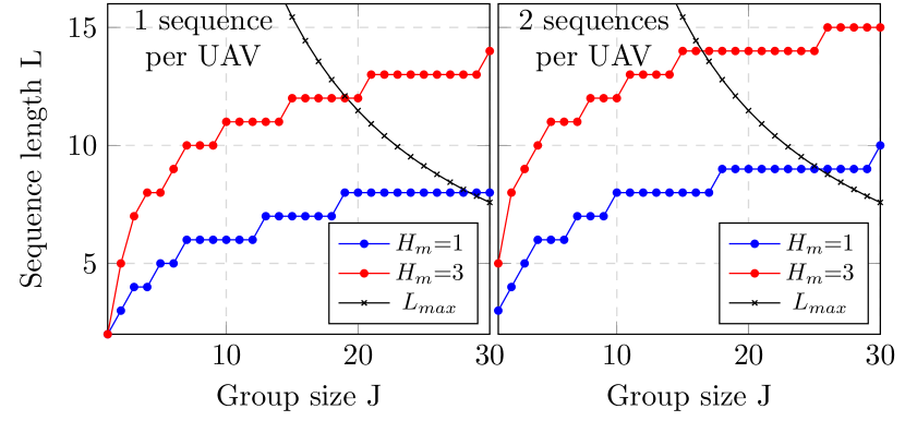
Figure 7: In black, $L_{max}$ for $p_{g}(J)$=0.999 and $T/\sigma_{T}=10^{4}$. In blue (red), minimum sequence length $L$ of a set with circular Hamming distance 1 (Hamming distance 3), that satisfies the cardinality constraints for a group of $J$ UAVs.

As mentioned in section VII-B, the variance $\sigma_{T}^{2}$ of the clock used in the UAVs determines the capacity of the identification system. To illustrate this, we analyse the case of groups composed of $J$ UAVs equipped with reasonably accurate clocks ($T/\sigma_{T}=10^{4}$). In Fig. 7, we plot in black the maximum sequence length $L_{max}$ that can be used by the identification system so that we have a probability $p_{g}\left(J\right)$ that all optical links can operate correctly (i.e., that any UAV can identify any other UAV). In blue, we plot the minimum sequence length $L$ of a set with circular Hamming distance 1, required to assign one sequence per UAV (left) and two sequences per UAV (right). In red, we plot the minimum sequence length $L$ of a set with circular Hamming distance 3 required to assign one sequence per UAV (left), and two sequences per UAV (right).

In the left image, we observe that for $L\geq 29$, the blue and red curves are above $L_{max}$. This means that given the clocks used by the UAVs, it is not possible to assign one distinct sequence per UAV and ensure that any UAV in the group will be able to identify any other UAV in the group with a probability of $p_{g}\left(J\right)$ or higher. In the right image where we assign two different sequences per UAV, this occurs for $L\geq 26$. If we want to assign two distinct sequences to every UAV and ensure any UAV in the group will be able to identify any other UAV in the group with a probability of $p_{g}\left(J\right)$ or higher, we will have to use clocks with higher accuracy.

On the left, we observe that for $20\leq J\leq 28$ only sets of sequences with circular Hamming distance 1 are able to satisfy the cardinality constraint, but any sets of sequences with circular Hamming distance 3 will fail to do so. Finally, groups of size $J\leq 19$ are able to use either sets of sequences with circular Hamming distance 1 or 3 and still satisfy the cardinality constraint.

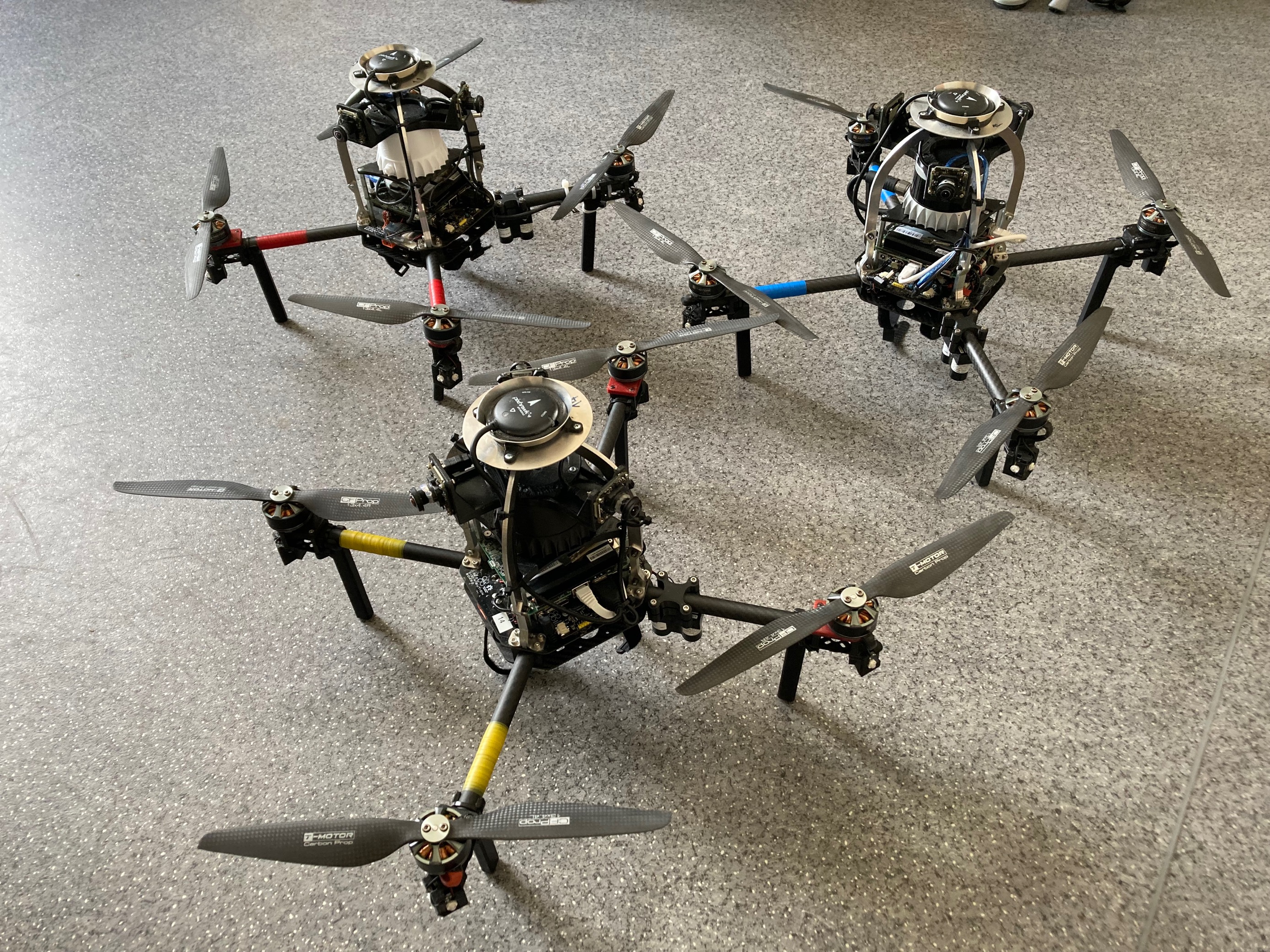
Figure 8: UAV platforms used in the experimental data acquisition. The frame is based on the Holybro X500 platform, with an arm length from the center of $0.245\text{\,}\mathrm{cm}$. Each unit is equipped with the UVDAR system, with three UV cameras and four pairs of UV LEDs. Each of the LED pairs is placed at the end of each arm of the UAV and the LEDs at $90\text{\,}\mathrm{\SIUnitSymbolDegree}$ horizontally from each other. The LEDs have a Lambertian radiation pattern and are rated at $1\text{\,}\mathrm{W}$ input power, although in our case, we are driving them at $200\text{\,}\mathrm{mW}$, producing cca $900\text{\,}\mathrm{mW}$ of radiometric power. Two of the cameras were aimed $70\text{\,}\mathrm{\SIUnitSymbolDegree}$ to the left and right from the central axis of the UAV, while the third was oriented backwards to cover the entirety of the horizontal surroundings.

VIII-C Camera interframe duration analysis

We have recorded the camera interframe duration of the UAV shown in Fig. 8 during 400 seconds, see Fig. 9 (top). The timings are recorded as they were reported by the camera driver used on the platforms. The camera frame rate was nominally set to 60 frames/s. The p.d.f. derived from the measurements histogram is plotted in blue in Fig. 9 (bottom) and the Laplace distribution with its parameters estimated using the maximum log-likelihood method is plotted in red. We observe an almost perfect match between both plots, and thus we conclude that the camera interframe duration follows a Laplace probability distribution. In Fig. 10, we observe the power spectrum of the temporal variations of the camera interframe duration. From the plot, we observe that the power spectrum is not flat and that the temporal variations of the camera interframe duration cannot be modelled as a white noise process.

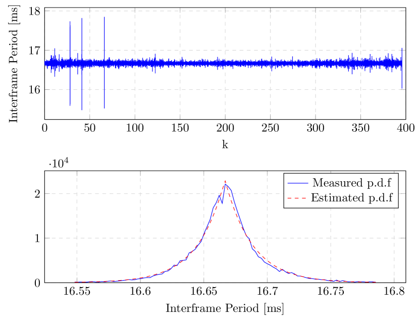
Figure 9: Interframe camera duration recorded (top). The p.d.f. of the interframe camera duration (bottom).

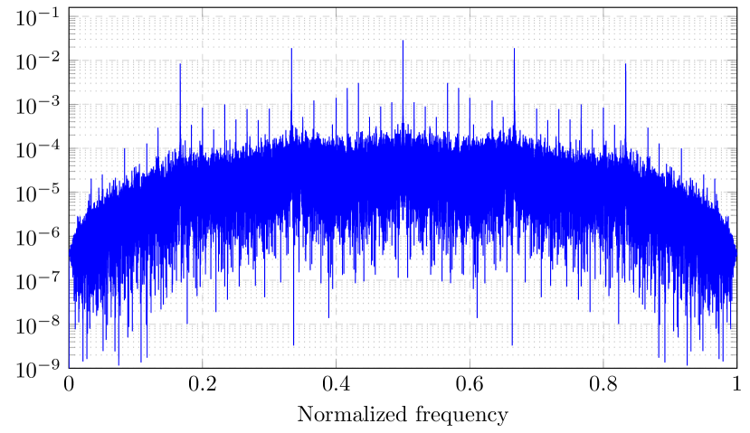
Figure 10: Power spectrum of the interframe camera period temporal variations.

VIII-D Static indoor testing

To continue investigating the effect of the clock signal impairments on the performance of the optical identification system, we perform the following indoor static experiment. We place two UAVs (UAV-0 and UAV-1) of the same model as before $5\text{\,}\mathrm{m}$ apart on the floor of the laboratory. The UAV-0 camera operates with a nominal frame rate of 60 frames/s, and points to UAV-1. The UAV-1 points one arm towards the UAV-0 camera, while two adjacent arms remain oriented parallel to the UAV-0 camera image plane. We name these LEDs in the order from left to right on their camera image as D0, D1, and D2.

The bit-rate of the blinking LEDs was $60.241\text{\,}\mathrm{Hz}$ due to hardware limitations of the microcontroller architecture used in the LED driver. This creates a difference in the period of less than $66.7\text{\,}\mathrm{\SIUnitSymbolMicro s}$ compared to the nominal camera period of $16.167\text{\,}\mathrm{ms}$ with the exposure time of the camera being set to $500\text{\,}\mathrm{\SIUnitSymbolMicro s}$. The precision of the crystal clock of the LED driver incurs an additional error that is several orders of magnitude lower that those of the other sources of error; it is thus considered negligible. Each LED emits an optical signal generated with a different binary sequence, see Fig. 4.

Regarding the optical signals emitter by the LEDs, we generate a set of binary sequences $f(\mathcal{S}^{7},0.5,3,3,1)$ with the algorithm described in section V. We then feed the binary stream generators (see Fig. 4) associated with the LEDs D0, D1, and D2 the binary sequences 0010111, 0011011, and 0011101. Then, we record the UAV-0 camera footage for $180\text{\,}\mathrm{s}$.

In this experiment, the pixels corresponding to the light emitted the LEDs get almost saturated when the LEDs are turned on because of the short distance between the UAVs. As a consequence, the resulting SNR at the receiver is high and the effects of the clock signal impairments and mismatch dominate the effects of the noise at the optical receiver.

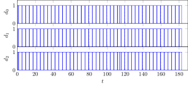
Figure 11: Classification success signals for $f(\mathcal{S}^{7},0.5,3,3,1)$ at $5\text{\,}\mathrm{m}$.

In Fig. 11, we plot, for each of the three LEDs, a binary signal that takes the value 1 when the binary sequence embedded in the optical signal is correctly classified, and 0 otherwise. The first thing we note in these plots is the presence of quasi periodic errors; these errors are generated by the mismatch between the transmitter and the receiver clock signals, as described in section VII.

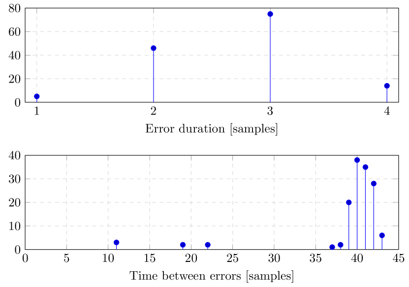
Figure 12: Error analysis for signal $f(\mathcal{S}^{7},0.5,3,3,1)$ at $5\text{\,}\mathrm{m}$.

To analyze these errors in more detail, we plot the histograms of their duration and of the time between errors measured from start-to-start in Fig. 12. From these histograms, we note two different types of errors; the first type of error is caused by noise at the receiver, and it has a duration of one single sample. The time between them does not follow any specific pattern. The second type of error is due to missing/duplicated bits caused by clock mismatches. In this experiment, they can last between two and four samples. The time between them is a random variable with a mean of around 40.6 samples and a variance of around 1.49 samples.

The histograms in Fig. 12 show the following: i) if the optical signals are generated with sequences with a length of 39 bits or larger, they will always be received with errors; ii) the clock signal mismatch is time-variant, which is why the time between errors caused by missing/duplicated bits varies mostly between 39-42 samples; and iii) at high SNR, the factor that mainly limits the performance of the optical identification system is the mismatch between the transmitter and receiver clocks.

VIII-E Dynamic outdoor testing

Finally, as proof of concept, we deployed outdoors a group of three UAVs (UAV-0, UAV-1, and UAV-2) equipped with the UVDAR system. We used binary sequences taken from the set generated with $f(\mathcal{S}^{14},3,3,0.5,1)$, and assigned one sequence to each arm of each UAV. Therefore, each UAV emitted four unique optical signals through its LEDs. We show in Fig. 13 a camera snapshot showing correctly classified markers. The UAVs flew autonomously according to a formation enforcement technique developed in our laboratory. The specifics of this formation enforcement system are beyond the scope of this work, but this experiment was also used to validate such formation algorithm. The UAVs were set to assume various specific relative formations in sequence, which was achieved with mutual relative localization using the UVDAR system as described in this paper. It worth noting that the ability to distinguish between the individual signals allowed the UAVs to identify each other and estimate relative orientations.

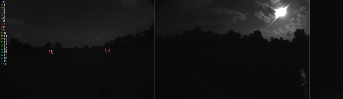
Figure 13: View left UVDAR camera of UAV-0 in outdoor flight experiment. The markers are correctly labeled based on the retrieved signal.

In this experiment, we recorded the content of the UAV-0 camera for $235\text{\,}\mathrm{s}$ with a nominal frame rate of 60 frames/s. The clock signal of the optical transmitters of all the UAVs operate with a nominal frequency of $60\text{\,}\mathrm{Hz}$. The trajectories shown in Fig. 14 present the relative motion of the UAV-1 and UAV-2 within the frame of the UAV-0 camera. This flight allowed us to test the visual identification system studied in this paper in a more challenging and realistic scenario.

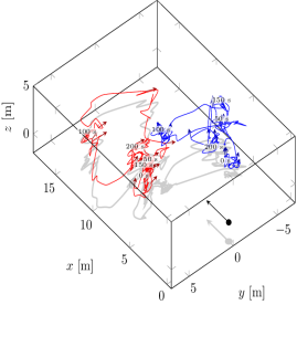
Figure 14: Trajectories of the UAV-1 (blue), UAV-2 (red) w.r.t. left UV camera (black) of UAV-0. Arrows signify the heading of the UAVs. The numbers along the trajectories indicate time.

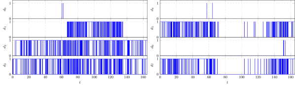
Figure 15: Successful classification signals for UAV-1 (left) and UAV-2 (right).

In Fig. 15, we plot the classification success signal for each individual LED of the UAV-1 (left column) and the UAV-2 (right column) by the left camera of UAV-0. This signal takes value 1 when the classification is successful, takes a zero value when there is an error in classification, or when the LED gets out of the UAV-0 camera FoV. From Fig. 15, we observe that usually only two LEDs per UAV are captured by the UAV-0 camera, although sometimes three LEDs can be captured simultaneously (see UAV-1 in the interval [70-135]s). We also note that the UAV-2 leaves the UAV-0 camera FoV and is lost for approximately $30\text{\,}\mathrm{s}$ during the experiment.

The detection success is significantly more erratic than in the prior testing with the static transmitter and receiver, since the motion of the UAVs affects the optical signal retrieval. Additionally, the distances between the transmitters and receivers were at times greater, and the contrast of the active LEDs in the image was slightly lower due to sunlight. Despite this, the classification success was good enough for the formation enforcement system to perform its function, which testifies of the practical applicability of the proposed identification system in real-world conditions.

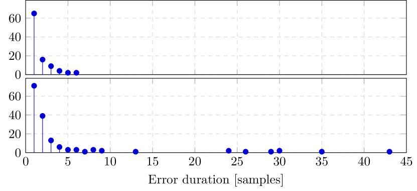
Figure 16: Error duration histograms for UAV-1 (top) and UAV-2 (bottom).

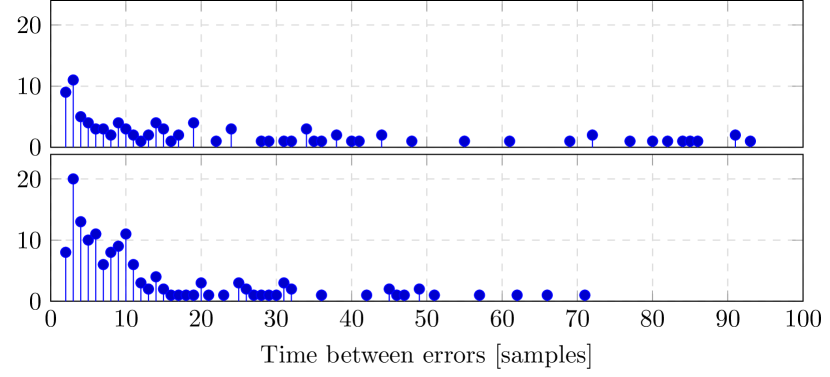
Figure 17: Time between error histograms for UAV-1 (top) and UAV-2 (bottom).

For both binary signals mentioned above, we plot in Fig. 16 the histograms of the duration of the errors observed. In Fig. 17, we plot the histograms of the time between the errors. The first thing that we note in Fig. 16 is that most of the errors for both UAVs last only one single sample. For UAV-1, single sample errors constitute 66.33$\%$ of the total errors. For UAV-1, single sample errors constitute 47.02$\%$ of the total errors. From Fig. 17, we also observe that errors occur more often; this is due to the larger distances (lower SNR) and the additional effect of the blurring and tracking errors. Despite the challenging conditions, the probability of correctly detecting UAV-1 is 0.9311 and that of detecting UAV-2 is 0.6327, while the errors appear in bursts of short duration (as long as the LoS is present). This shows that this identification system can operate with good performance in real scenarios.

Finally, we present a video of the experiment just described above in the following link, and in Fig. 18 we observe some snapshots of the video.

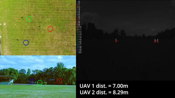
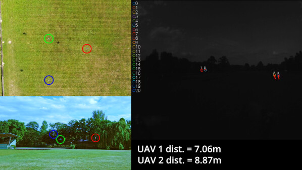
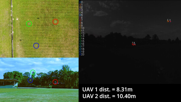
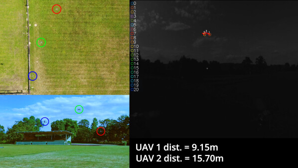
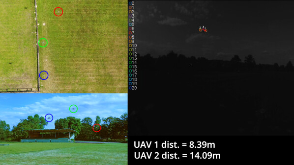
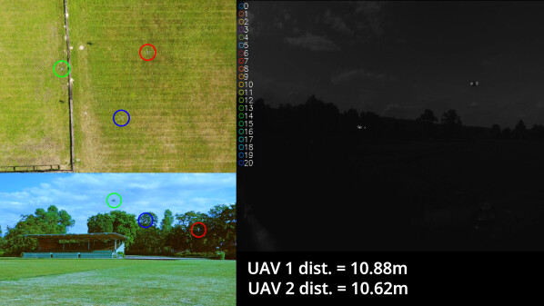
Figure 18: Snapshots from the outdoor experimental testing video. UAV-0 (red), UAV-1 (green), and UAV-2 (blue). The time difference between snapshots is $30\text{\,}\mathrm{s}$.

IX Conclusion

In this paper, we have studied in detail the theoretical and practical aspects of the camera-based optical identification system for UAVs, called UVDAR. We have shown how to optimize the optical signals emitted by the UAVs in order to maximize the number of detectable UAVs and minimize identification time. We have also demonstrated with theoretical analysis and through experiments that clock signal mismatches are some of the main elements limiting the visual identification system capacity. We have tested the visual identification system both indoors and outdoors and shown that it can operate with reasonable performance and we have also characterized its error behaviour. The achieved results can be directly exploited for the optimization of the performance of visual-based localization and identification systems, such as UVDAR, for increased robustness against tracking errors and for evaluating the capacity of this optical system in serving as the basis for an optical communication network for UAVs.

Appendix A Hamming Distance Elimination

In this section, we describe an iterative suboptimum solution for the optimization problem (33)-(V-A4). At each iteration, a candidate set is constructed by randomly discarding sequences from the input set. After a number of predefined iterations, the algorithm selects the candidate set with the highest cardinality.

Let us start by considering a set $\mathcal{S}^{L}$ of binary sequences of length $L$. We store the subindex $k$ of the sequence $\mathbf{b}_{k}\in\mathcal{S}^{L}$ in the $k$th entry of the vector $\mathbf{v}$, i.e., $[\mathbf{v}]_{k}=k$, for $k=1,2,\cdots,|\mathcal{S}^{L}|$. We can solve (63) with the following iterative algorithm, where at iteration $i$, we construct the following vector:

$$\mathbf{w}_{i}=\mathbf{P}_{i}\mathbf{v},$$ (63)

where $\mathbf{P}_{i}$ is a random permutation matrix. Then, we form the Hamming distance matrix $\mathbf{H}(\mathbf{P}_{i})$ where $[\mathbf{H}(\mathbf{P}_{i})]_{m,n}=H_{c}(\mathbf{b}_{[\mathbf{w}_{i}]_{m}},\mathbf{b}_{[\mathbf{w}_{i}]_{n}})$, see (19). We then create a binary vector $\mathbf{f}_{i}$ of length $|\mathcal{S}|$ with all entries initiated with value ’1’. Starting at the first row, we analyze this matrix. We check entry by entry from the column $m=n+1$ up to the last. If $[\mathbf{f}_{i}]_{m}=1$, we analyze this row, otherwise we skip it and move to the next one. If $[\mathbf{f}_{i}]_{n}=1$ and $[\mathbf{H}(\mathbf{P}_{i})]_{m,n}\geq H_{m}$, then we do nothing. If $[\mathbf{f}_{i}]_{n}=1$ and $[\mathbf{H}(\mathbf{P}_{i})]_{m,n}<H_{m}$, we set $[\mathbf{f}_{i}]_{n}=0$. If $[\mathbf{f}_{i}]_{n}=0$, we skip this entry. When we finish analyzing this row, we proceed to analyze the next row with the same procedure. Once we finish analyzing $\mathbf{H}(\mathbf{P}_{i})$, we generate a new random permutation matrix $\mathbf{P}_{i+1}$ and repeat the process until we run the desired number of algorithm iterations $I$. Finally, we select the vector $\{\mathbf{f}_{i}\}_{i=1}^{I}$ with the largest norm as the suboptimal solution for the optimization problem (33)-(V-A4).

The optimization problem (33)-(V-A4) is a combinatorial problem. The only way to actually be sure to obtain the optimum solution is to run the algorithm described in this appendix for all the possible $|\mathcal{S}^{L}|!$ permutation matrices $\mathbf{P}$. However, $|\mathcal{S}^{L}|!$ is, in general, an astronomically large number, then we cannot explore the full search space of (33)-(V-A4) and we can only obtain a suboptimum solution. As the number of iterations $I$ increases, so does the probability that the obtained vector $\mathbf{f}$ is the optimum solution for (33)-(V-A4).

Appendix B Classifier

Each classifier has $M$ parallel correlator filters. The $m$th correlator is tuned to the binary sequence contained in the $m$th row of the dictionary $\mathbf{D}$. Thus, the output of the $m$th correlator of the classifier associated to the time series $y_{j,n}$ of the $j$th UAV is given by:

$$w_{j,n}[k] = \frac{1}{L}\max\left(\mathbf{C}(f_{bip}([\mathbf{D}]_{m}))f_{bip}(\mathbf{y}_{j,n}[k])\right),$$ (64)

$$\mathbf{y}_{j,n}[k] = [y_{j,n}[k],y_{j,n}[k-1],\cdots,y_{j,n}[k-L+1]]^{\mathrm{T}},$$

where $[\mathbf{D}]_{m}$ is the $m$th row of the dictionary matrix $\mathbf{D}$, $f_{bip}(\cdot)$ is a function that maps the unipolar binary variable $a\in\{0,1\}$ to the bipolar binary variable $f_{bip}(a)\in\{-1,+1\}$, where $\mathbf{C}([\mathbf{D}]_{m})$ is a square circulant matrix formed with the sequence $[\mathbf{D}]_{m}$. Finally, the outputs of the $M$ correlators are fed into the classifying layer:

$$z_{j,n}[k]=\begin{cases}\operatorname*{arg\,max}_{j}\{w_{j,n}[k]\}\quad\,\mathrm{if}\quad\,\max_{j}\{w_{j,n}[k]\}\geq\eta_{d}\\ -1\quad\quad\quad\quad\quad\quad\quad\quad\,\mathrm{otherwise}\end{cases}$$ (65)

where $\eta_{d}$ is the detection threshold. If $z_{n}[k]\neq-1$, then $z_{j,n}[k]$ contains the estimation of the identification number of the sequence contained in the time series $y_{j,n}$. On the other hand, if $z_{n}[k]=-1$, then the classifier assumes at time $k$ that $y_{j,n}$ is not generated by any binary sequence contained in the dictionary $\mathbf{D}$. This can be due to erroneous bits that modified the time series $y_{j,n}$ or can also be because $y_{j,n}$ is generated by random sources of light external to the UAV group (e.g., sun reflections or blinking LEDs for external systems).

Appendix C SNR and bit error probability

Following a similar analysis as in [30, 31] and using (38), we can show that the probability distribution of $a[k]$ in (9) is:

$$f_{a}(x_{a})=\left(\frac{T-\tau_{e}}{T}\right)\delta(x_{a}-1)+\frac{\tau_{e}}{T}$$ (66)

with $\mathbb{E}[a[k]]=1-\frac{\tau_{e}}{2T}$ and $\mathbb{E}[a^{2}[k]]=1-\frac{2\tau_{e}}{3T}$. $x_{a}\in[0,1]$ is a uniform random variable that represents the random phase shift between the transmitter and receiver. Thus, the SNR (III) becomes:

$$\gamma_{k}=\frac{h^{2}_{k}P^{2}\tau_{e}^{2}\left(\left(1-\frac{\tau_{e}}{3T}\right)\mathbb{E}\left[s[k_{t}]\right]+\frac{\tau_{e}}{3T}\mathbb{E}\left[s[k_{t}]s[k_{t}+1]\right]\right)}{\tau_{e}^{2}{d}_{k}^{2}+\tau_{e}(\sigma_{th,1}^{2}+\alpha{d}_{k}+\alpha h_{k}P\mathbb{E}[s[k_{t}]])+\sigma_{th,2}^{2}},$$ (67)

and the erroneous bit probability is:

$$\mathrm{p}_{b} = \mathrm{Pr}\left(x_{k}>\eta_{b}|s_{k}=0,s_{k+1}=0\right)\mathrm{Pr}\left(s_{k}=0,s_{k+1}=0\right)$$

$$+ \mathrm{Pr}\left(x_{k}>\eta_{b}|s_{k}=0,s_{k+1}=1\right)\mathrm{Pr}\left(s_{k}=0,s_{k+1}=1\right)$$

$$+ \mathrm{Pr}\left(x_{k}<\eta_{b}|s_{k}=1,s_{k+1}=0\right)\mathrm{Pr}\left(s_{k}=1,s_{k+1}=0\right)$$

$$+ \mathrm{Pr}\left(x_{k}<\eta_{b}|s_{k}=1,s_{k+1}=1\right)\mathrm{Pr}\left(s_{k}=1,s_{k+1}=1\right)$$

where $\eta_{b}$ is the binarization threshold, $x_{k}$ is the short notation for $x_{\ell}[k]$ in (8), and:

$$\mathrm{Pr}\left(s_{k}=a,s_{k+1}=b\right)=\mathrm{Pr}\left(s_{k}=a|,s_{k+1}=b\right)\mathrm{Pr}\left(s_{k+1}=b\right)$$ (69)

with $\mathrm{Pr}\left(s_{k+1}=1\right)=\frac{\sum_{k}k|\mathcal{E}_{k}|}{L\sum_{k}|\mathcal{E}_{k}|}$ and $\mathrm{Pr}\left(s_{k+1}=0\right)=1-\mathrm{Pr}\left(s_{k+1}=1\right)$. The conditional probabilities in (69) must be calculated numerically from the set of binary sequences in the dictionary $\mathbf{D}$. The conditional probabilities in (C) must be calculated considering the optical channel described in section III.

ORCID

Daniel Bonilla Licea${}^{\href{https://orcid.org/0000-0002-1057-816X}{\mbox{\scalerel*{ \leavevmode\hbox to256pt{\vbox to256pt{\text{[drawing]}}} }{|}}}}$: 0000-0002-1057-816X
Viktor Walter${}^{\href{https://orcid.org/0000-0001-8693-6261}{\mbox{\scalerel*{ \leavevmode\hbox to256pt{\vbox to256pt{\text{[drawing]}}} }{|}}}}$: 0000-0001-8693-6261
Mounir Ghogho${}^{\href{https://orcid.org/0000-0002-0055-7867}{\mbox{\scalerel*{ \leavevmode\hbox to256pt{\vbox to256pt{\text{[drawing]}}} }{|}}}}$: 0000-0002-0055-7867
Martin Saska${}^{\href{https://orcid.org/0000-0001-7106-3816}{\mbox{\scalerel*{ \leavevmode\hbox to256pt{\vbox to256pt{\text{[drawing]}}} }{|}}}}$: 0000-0001-7106-3816

Daniel Bonilla Licea received his M.Sc. degree in 2011 from the Centro de Investigación y Estudios Avanzados (CINVESTAV), Mexico City. From May 2011 until June 2012, he worked as an intern in the signal processing team of Intel Labs in Guadalajara, Mexico. He received his PhD degree in 2016 from the University of Leeds, U.K. In 2016 he was invited for a short research visit at the Centre de Recherche en Automatique de Nancy (CRAN), France. In 2017, he collaborated in a research project with the Centro de Investigación en Computacion (CIC) in Mexico. From 2017 to 2020, he held a postdoctoral position at the International University of Rabat, Morocco. Currently, he holds a postdoctoral position at the Czech Technical University in Prague, Czech Republic. His primary research interests include signal processing and communications-aware robotics.

Viktor Walter received his MSc. degree at Brno University of Technology in 2016 and entered the Multi-Robot Systems (MRS) group at the Czech Technical University in Prague the same year for his PhD studies. In 2017 and 2018, he visited the CNRS Laboratory of Analysis and Architecture of Systems (LAAS) in Toulouse, where he worked in the Robotics and Interactions (RIS) group under professor Antonio Franchi. Currently, he works as a researcher and PhD student at the Czech Technical University in Prague in the MRS group led by Martin Saska. His research concerns vision-based mutual relative localization of UAVs and other applications of computer vision on UAVs. He developed and maintains the UltraViolet Direction And Ranging (UVDAR) system used by MRS and other research teams for real-world cooperative UAV flights in arbitrary environments.

Mounir Ghogho has received the M.Sc. degree in 1993 and the PhD degree in 1997 from the National Polytechnic Institute of Toulouse, France. He was an EPSRC Research Fellow with the University of Strathclyde (Scotland), from Sept 1997 to Nov 2001. In Dec 2001, he joined the school of Electronic and Electrical Engineering at the University of Leeds (England), where he was promoted to full Professor in 2008. While still affiliated with the University of Leeds, in 2010 he joined the International University of Rabat where he is currently Dean of the College of Doctoral Studies and Director of TICLab (ICT Research Laboratory). He is a Fellow of IEEE and AAIA (Asia-Pacific AI Association), a recipient of the 2013 IBM Faculty Award, and a recipient of the 2000 UK Royal Academy of Engineering Research Fellowship. He is the co-founder and co-director of the CNRS-associated International Research lab DataNet, in the field of Big Data and artificial intelligence. His research interests are in Machine Learning, Signal Processing and Wireless Communication. He has coordinated around 20 research projects and supervised over 30 PhD students in the UK and Morocco. He served as Associate Editor of many journals including the IEEE Signal Processing Magazine and the IEEE Transactions on Signal Processing.

Martin Saska received his MSc. degree at Czech Technical University in Prague, 2005, and his Ph.D. degree at University of Wuerzburg, Germany, within the PhD program of Elite Network of Bavaria, 2009. Since 2009, he is a research fellow at Czech Technical University in Prague, where he founded and heads the Multi-robot Systems lab (http://mrs.felk.cvut.cz/) and co-founded Center for Robotics and Autonomous Systems with more than 70 researchers cooperating in robotics (https://robotics.fel.cvut.cz/cras/). He was a visiting scholar at University of Illinois at Urbana-Champaign, USA in 2008, and at University of Pennsylvania, USA in 2012, 2014 and 2016, where he worked with Vijay Kumar’s group within GRASP lab. He is an author or co-author of ¿150 publications in peer-reviewed conferences with multiple best paper awards and more ¿40 publications in impacted journals, including IJRR, AURO, JFR, ASC, EJC, with ¿4000 citations indexed by Scholar and H-index 35. His team won multiple robotic challenges in MBZIRC 2017, MBZIRC 2020, and DARPA SubT competitions (http://mrs.felk.cvut.cz/projects/mbzirc, http://mrs.felk.cvut.cz/mbzirc2020, http://mrs.felk.cvut.cz/projects/darpa).

References

- [1] Q. Ali, N. Gageik, and S. Montenegro, “A review on distributed control of cooperating mini uavs,” International Journal of Artificial Intelligence & Applications, vol. 5, pp. 1–13, 2014.
- [2] J. Vilca, L. Adouane, and Y. Mezouar, “Adaptive leader-follower formation in cluttered environment using dynamic target reconfiguration,” in Distributed Autonomous Robotic Systems, N.-Y. Chong and Y.-J. Cho, Eds. Tokyo: Springer Japan, 2016, pp. 237–254.
- [3] T. Chen, Q. Gao, and M. Guo, “An improved multiple uavs cooperative flight algorithm based on leader follower strategy,” in 2018 Chinese Control And Decision Conference (CCDC), 2018, pp. 165–169.
- [4] D. A. Mercado, R. Castro, and R. Lozano, “Quadrotors flight formation control using a leader-follower approach,” in 2013 European Control Conference (ECC), 2013, pp. 3858–3863.
- [5] T. K. et al., “A practical multirobot localization system,” J. Intell. Robot. Syst., vol. 76, p. 539–562, 2014.
- [6] M. S. et al., “System for deployment of groups of unmanned micro aerial vehicles in gps-denied environments using onboard visual relative localization,” Auton. Robots, vol. 41, no. 4, pp. 919–944, 2017.
- [7] A. Censi, J. Strubel, C. Brandli, T. Delbruck, and D. Scaramuzza, “Low-latency localization by active led markers tracking using a dynamic vision sensor,” in 2013 IEEE/RSJ International Conference on Intelligent Robots and Systems, 2013, pp. 891–898.
- [8] V. Walter, M. Saska, and A. Franchi, “Fast mutual relative localization of uavs using ultraviolet led markers,” in 2018 International Conference on Unmanned Aircraft Systems (ICUAS), 2018, pp. 1217–1226.
- [9] V. Walter, N. Staub, M. Saska, and A. Franchi, “Mutual localization of uavs based on blinking ultraviolet markers and 3d time-position hough transform,” in 2018 IEEE 14th International Conference on Automation Science and Engineering (CASE), 2018, pp. 298–303.
- [10] V. Walter, N. Staub, A. Franchi, and M. Saska, “Uvdar system for visual relative localization with application to leader–follower formations of multirotor uavs,” IEEE Robotics and Automation Letters, vol. 4, no. 3, pp. 2637–2644, 2019.
- [11] P. Petráček, V. Walter, T. Báča, and M. Saska, “Bio-inspired compact swarms of unmanned aerial vehicles without communication and external localization,” Bioinspiration & Biomimetics, vol. 16, no. 2, p. 026009, dec 2020. [Online]. Available: https://doi.org/10.1088/1748-3190/abc6b3
- [12] N. T. Le, M. Hossain, and Y. M. Jang, “A survey of design and implementation for optical camera communication,” Signal Processing: Image Communication, vol. 53, pp. 95–109, 2017. [Online]. Available: https://www.sciencedirect.com/science/article/pii/S0923596517300188
- [13] N. Saeed, S. Guo, K.-H. Park, T. Y. Al-Naffouri, and M.-S. Alouini, “Optical camera communications: Survey, use cases, challenges, and future trends,” Physical Communication, vol. 37, p. 100900, 2019. [Online]. Available: https://www.sciencedirect.com/science/article/pii/S1874490719304859
- [14] I. Takai, S. Ito, K. Yasutomi, K. Kagawa, M. Andoh, and S. Kawahito, “Led and cmos image sensor based optical wireless communication system for automotive applications,” IEEE Photonics Journal, vol. 5, no. 5, pp. 6 801 418–6 801 418, 2013.
- [15] I. Takai, T. Harada, M. Andoh, K. Yasutomi, K. Kagawa, and S. Kawahito, “Optical vehicle-to-vehicle communication system using led transmitter and camera receiver,” IEEE Photonics Journal, vol. 6, no. 5, pp. 1–14, 2014.
- [16] Y. H. Kim, W. A. Cahyadi, and Y. H. Chung, “Experimental demonstration of vlc-based vehicle-to-vehicle communications under fog conditions,” IEEE Photonics Journal, vol. 7, no. 6, pp. 1–9, 2015.
- [17] T. Nguyen, A. Islam, and Y. M. Jang, “Region-of-interest signaling vehicular system using optical camera communications,” IEEE Photonics Journal, vol. 9, no. 1, pp. 1–20, 2017.
- [18] M. R. Soares, N. Chaudhary, E. Eso, O. I. Younus, L. Nero Alves, and Z. Ghassemlooy, “Optical camera communications with convolutional neural network for vehicle-tovehicle links,” in 2020 12th International Symposium on Communication Systems, Networks and Digital Signal Processing (CSNDSP), 2020, pp. 1–6.
- [19] T. Nguyen, A. Islam, T. Hossan, and Y. M. Jang, “Current status and performance analysis of optical camera communication technologies for 5g networks,” IEEE Access, vol. 5, pp. 4574–4594, 2017.
- [20] P. Luo, M. Zhang, Z. Ghassemlooy, S. Zvanovec, S. Feng, and P. Zhang, “Undersampled-based modulation schemes for optical camera communications,” IEEE Communications Magazine, vol. 56, no. 2, pp. 204–212, 2018.
- [21] D. T. Nguyen, Y. Chae, and Y. Park, “Enhancement of data rate and packet size in image sensor communications by employing constant power 4-pam,” IEEE Access, vol. 6, pp. 8000–8010, 2018.
- [22] A. Ahmad, D. Bonilla Licea, G. Silano, T. Baca, and M. Saska, “PACNav: A Collective Navigation Approach for UAV Swarms Deprived of Communication and External Localization,” Bioinspiration & Biomimetics, October 2022. [Online]. Available: https://iopscience.iop.org/article/10.1088/1748-3190/ac98e6
- [23] J. Horyna, V. Walter, and M. Saska, “Uvdar-com: Uv-based relative localization of uavs with integrated optical communication,” in 2022 International Conference on Unmanned Aircraft Systems (ICUAS), 2022, pp. 1302–1308.
- [24] V. Walter, N. Staub, A. Franchi, and M. Saska, “Uvdar system for visual relative localization with application to leader–follower formations of multirotor uavs,” IEEE Robotics and Automation Letters, vol. 4, no. 3, pp. 2637–2644, July 2019.
- [25] F. Novák, V. Walter, P. Petráček, T. Báča, and M. Saska, “Fast collective evasion in self-localized swarms of unmanned aerial vehicles,” Bioinspiration & Biomimetics, vol. 16, no. 6, p. 066025, nov 2021. [Online]. Available: https://doi.org/10.1088/1748-3190/ac3060
- [26] F. Novák, “State estimation of an unmanned surface vehicle by an unmanned multirotor helicopter,” 2022. [Online]. Available: http://hdl.handle.net/10467/100876
- [27] V. Walter, M. Vrba, and M. Saska, “On training datasets for machine learning-based visual relative localization of micro-scale UAVs,” in 2020 IEEE International Conference on Robotics and Automation (ICRA), Aug 2020, pp. 10 674–10 680.
- [28] T. Nguyen, N. T. Le, and Y. M. Jang, “Asynchronous scheme for unidirectional optical camera communications (occ),” in 2014 Sixth International Conference on Ubiquitous and Future Networks (ICUFN), 2014, pp. 48–51.
- [29] W. Hu, H. Gu, and Q. Pu, “Lightsync: Unsynchronized visual communication over screen-camera links,” in Proceedings of the 19th Annual International Conference on Mobile Computing &; Networking, ser. MobiCom ’13. New York, NY, USA: Association for Computing Machinery, 2013, p. 15–26. [Online]. Available: https://doi.org/10.1145/2500423.2500437
- [30] W. Mao and J. Kahn, “Free-space heterochronous imaging reception of multiple optical signals,” IEEE Transactions on Communications, vol. 52, no. 2, pp. 269–279, 2004.
- [31] D. Messerschmitt, “Synchronization in digital system design,” IEEE Journal on Selected Areas in Communications, vol. 8, no. 8, pp. 1404–1419, 1990.
- [32] C. W. Chow, C. H. Yeh, Y. F. Liu, and P. Y. Huang, “Mitigation of optical background noise in light-emitting diode (led) optical wireless communication systems,” IEEE Photonics Journal, vol. 5, no. 1, pp. 7 900 307–7 900 307, 2013.
- [33] J. Kahn and J. Barry, “Wireless infrared communications,” Proceedings of the IEEE, vol. 85, no. 2, pp. 265–298, 1997.
- [34] “BP365 near-uv bandpass filter,” https://midopt.com/filters/bp365/, accessed: 2022-03-10.
- [35] S. Hranilovic and F. Kschischang, “A pixelated mimo wireless optical communication system,” IEEE Journal of Selected Topics in Quantum Electronics, vol. 12, no. 4, pp. 859–874, 2006.
- [36] R. Singh, T. O’Farrell, and J. P. R. David, “An enhanced color shift keying modulation scheme for high-speed wireless visible light communications,” Journal of Lightwave Technology, vol. 32, no. 14, pp. 2582–2592, 2014.
- [37] M. Uysal, C. Capsoni, Z. Ghassemlooy, A. Boucouvalas, and E. Udvary, Optical Wireless Communications. Springer, 2016.
- [38] T. Yamazato, M. Kinoshita, S. Arai, E. Souke, T. Yendo, T. Fujii, K. Kamakura, and H. Okada, “Vehicle motion and pixel illumination modeling for image sensor based visible light communication,” IEEE Journal on Selected Areas in Communications, vol. 33, no. 9, pp. 1793–1805, 2015.
- [39] T. Kasashima, T. Yamazato, H. Okada, T. Fujii, T. Yendo, and S. Arai, “Interpixel interference cancellation method for road-to-vehicle visible light communication,” in 2013 IEEE 5th International Symposium on Wireless Vehicular Communications (WiVeC), 2013, pp. 1–5.
- [40] D. Vuong and M. Yoo, “Interpixel interference mitigation in visible light communication using image sensor,” IEEE Access, vol. 6, pp. 45 543–45 551, 2018.
- [41] S. Yoshizawa, S. Handa, F. Sasamori, and O. Takyu, “A simple but effective approach for visible light beacon-based positioning systems with smartphone,” in 2016 IEEE 12th International Colloquium on Signal Processing Its Applications (CSPA), 2016, pp. 32–35.
- [42] C. L. Lim, K. S. Lee, H. Wang, H. Weatherspoon, and A. Tang, “Packet clustering introduced by routers: Modeling, analysis and experiments,” in 2014 48th Annual Conference on Information Sciences and Systems (CISS), 2014, pp. 1–6.
- [43] L. Li, P. Hu, C. Peng, G. Shen, and F. Zhao, “Epsilon: A visible light based positioning system,” in 11th USENIX Symposium on Networked Systems Design and Implementation (NSDI 14). Seattle, WA: USENIX Association, Apr. 2014, pp. 331–343. [Online]. Available: https://www.usenix.org/conference/nsdi14/technical-sessions/presentation/li
- [44] S. Shimada, H. Hashizume, and M. Sugimoto, “Indoor positioning using reflected light and a video camera,” in 2018 International Conference on Indoor Positioning and Indoor Navigation (IPIN), 2018, pp. 1–8.
- [45] J. K. Kwon, “Inverse source coding for dimming in visible light communications using nrz-ook on reliable links,” IEEE Photonics Technology Letters, vol. 22, no. 19, pp. 1455–1457, 2010.
- [46] P. E. Hart, “How the hough transform was invented [dsp history],” IEEE Signal Processing Magazine, vol. 26, no. 6, pp. 18–22, 2009.
- [47] V. Pless, Introduction to the Theory of Error-Correcting Codes. John Wiley & Sons, Ltd, 1998.