Robust and Scalable Bayesian Online Changepoint Detection

Abstract

This paper proposes an online, provably robust, and scalable Bayesian approach for changepoint detection. The resulting algorithm has key advantages over previous work: it provides provable robustness by leveraging the generalised Bayesian perspective, and also addresses the scalability issues of previous attempts. Specifically, the proposed generalised Bayesian formalism leads to conjugate posteriors whose parameters are available in closed form by leveraging diffusion score matching. The resulting algorithm is exact, can be updated through simple algebra, and is more than 10 times faster than its closest competitor.

1 Introduction

Changepoint (CP) detection is the task of identifying sudden changes in the statistical properties of a data stream. The methods to detect CPs are used in applications including systems health monitoring (Stival et al., 2022; Yang et al., 2006), financial data (Kim et al., 2022; Kummerfeld & Danks, 2013), climate change (Reeves et al., 2007; Itoh & Kurths, 2010), and cyber security (Hallgren et al., 2022). Existing approaches include likelihood ratio methods such as the parametric method CUSUM (Page, 1954) or Change Finder methods (Kawahara & Sugiyama, 2009), to Bayesian methods such as in Chib (1998); Fearnhead (2006).

Detecting CPs in an online fashion is an even more challenging task, but can allow practitioners to act on these systems in real-time. In a Bayesian context, the most popular method is Bayesian online changepoint detection (BOCD) (Adams & MacKay, 2007; Fearnhead & Liu, 2007). Here, the data stream is assumed to come from one of several different underlying distributions; and the goal is to quantify our uncertainty over the most recent time at which the data distribution changed. BOCD has many desirable properties: it is suitable for multivariate data and has the capacity to quantify uncertainty. However, it also has a significant flaw inherited from Bayesian inference: it is not robust under outliers or model misspecification. This can lead to failures, where most data points inferred to be CPs are simply mild heterogeneities in the data. This is a significant problem, and can causes practitioners to act on safety-critical systems based upon an erroneously declared CPs.

The lack of robustness in Bayesian methods has recently come to the forefront, and various strategies have been proposed to address it. Arguably the most successful amongst these have been generalised Bayesian methods (see e.g. Bissiri et al., 2016; Jewson et al., 2018; Knoblauch et al., 2022). Building on these ideas, Knoblauch et al. (2018) introduced the first robust version of BOCD using generalised Bayesian inference based on $\beta$-divergences ($\beta$-BOCD).

While the resulting algorithm is generally applicable and provides robustness, it has a major drawback that has severely impeded its broader use: it is not scalable. This is mainly due to the intractability of the generalised posterior and predictive distributions, which require multiple variational approximations to be performed at each time point. As a result, $\beta$-BOCD is practically infeasible if one is interested in online methods for high-frequency data, or if one deals with a constrained computational budget.

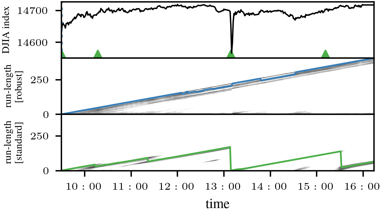
Figure 1: Twitter Flash Crash. The run-length is the time since the last changepoint (CP). Top: Jow Dones Index with Maximum a posteriori CPs detected by standard BOCD marked as ${\color[rgb]{77,175,74}\blacktriangle}$. Middle & Bottom: run-length posteriors of ${\mathcal{D}}_{m}$-BOCD with most likely run-length in blue and of standard BOCD in green. Standard BOCD incorrectly detects a CP, ${\mathcal{D}}_{m}$-BOCD does not.

This paper proposes a new generalised Bayesian inference scheme based on diffusion score matching (Barp et al., 2019), which is effectively a weighted version of the original score-matching divergence of Hyvärinen (2006). If the weights are chosen appropriately, the resulting posteriors are provably robust, and the corresponding CP detection algorithm, denoted ${\mathcal{D}}_{m}$-BOCD, is also robust to outliers. This is illustrated in Figure 1 on the value of the Dow Jones Industrial Average (DJIA) on the day of the ‘Twitter flash crash’ on 17/04/2013: standard BOCD falsely identifies $3$ CPs, whilst ${\mathcal{D}}_{m}$-BOCD correctly identifies no CPs.

Additionally—and unlike posteriors based on the $\beta$-divergence—${\mathcal{D}}_{m}$-posteriors also have a conjugacy property for likelihoods of the exponential family so long as the prior is chosen to be a normal, truncated normal, or any other squared exponential distribution. This makes ${\mathcal{D}}_{m}$-BOCD very fast: specifically, it ensures that all posteriors used in the algorithm can be updated exactly and efficiently through elementary vector and matrix calculations. If one uses the pruning strategies for the CP posterior proposed in Adams & MacKay (2007), the computational complexity of our algorithm is $\mathcal{O}(T(d^{2}+p^{2}))$; where $T$ is the length of the data stream, $d$ is the dimension of the observations, and $p$ is the number of model parameters. This is the same computational complexity as the original BOCD algorithm. This also makes ${\mathcal{D}}_{m}$-BOCD more than $10$ times faster than $\beta$-BOCD in our numerical experiments.

Beyond that, ${\mathcal{D}}_{m}$-BOCD has benefits that make it more attractive than standard BOCD even from a purely computational point of view in certain settings. For example, when modelling $d$-dimensional observations with non-Gaussian exponential family distributions, we can obtain conjugate ${\mathcal{D}}_{m}$-posteriors, even though no conjugate posteriors exist in the standard Bayesian case.

In summary, we make two key contributions:

• We derive and propose the ${\mathcal{D}}_{m}$-posterior; proving its robustness and closed form updates in the process;

• We use this posterior for BOCD, leading to the first algorithm that is both robust and scalable.

The remainder of the paper is structured as follows: Section 2 reviews BOCD and generalised Bayesian inference. Section 3 derives the robustness and scalability properties of ${\mathcal{D}}_{m}$-posteriors, and integrates them with BOCD. We then validate our approach experimentally in Section 4.

2 Background

Our method merges generalised Bayesian posteriors based on diffusion score matching with the BOCD algorithm. Here, we provide a short explanation of the concepts relevant for understanding this interface.

2.1 Bayesian Online Changepoint Detection (BOCD)

Let $x_{1:T}$ be a sequence of observations $x_{1},x_{2},\dots,x_{T}$, where $x_{t}\in{\mathcal{X}}\subseteq{\mathbb{R}}^{d}$ for the time index $t\in\{1,\ldots,T\}$. Throughout, $x_{1:T}$ follows the product partition model of Barry & Hartigan (1993): the data is partitioned through a sequence of changepoints (CPs) $0=\tau_{1}<\tau_{2}<\dots$ so that the $i$-th segment is $x_{\tau_{i}:\tau_{i+1}-1}$, and data within the $i$-th segment is independently and identically distributed (i.i.d.) conditional on $\tau_{i},\tau_{i+1}$. In the model underlying BOCD, the data in each segment is modelled with the same model class $\{p_{\theta}:\theta\in\Theta\}$, but with a different parameter for each segment. The key insight for this model, reached independently by both Adams & MacKay (2007) and Fearnhead & Liu (2007), is that Bayesian inference can be made online and efficiently if, at time $t$, one only tracks a posterior distribution over the most recent CP. Instead of defining a prior and posterior over the CPs directly, BOCD therefore seeks to infer the so-called run-length $r_{t}$ of the current segment—the amount of time since the most recent CP.

The remainder of this section details the hierarchical Bayesian model underlying the BOCD construction. Firstly, the approach uses a conditional prior on the run-length:

$$\textstyle r_{t}|r_{t-1} \textstyle\sim H(r_{t}|r_{t-1}).$$ (Conditional prior on run-length)

Since at time $t$ we either have a new CP ($r_{t}=0$) or the current segment continues ($r_{t}=r_{t-1}+1$), $H(r_{t}|r_{t-1})$ has positive probability mass only for $r_{t}\in\{0,r_{t-1}+1\}$. See Wilson et al. (2010) for a broader discussion of prior selection. Conditional on $r_{t}$, all data points $x_{t^{\prime}}$ from the same segment $(t-r_{t}):t$ so that $t^{\prime}\in\{t-r_{t},t-r_{t}+1,\dots,t\}$ are then modelled as i.i.d. from $p_{\theta}$ via

$$\textstyle\theta \textstyle\sim\pi(\theta)$$ (Parameter prior),

$$\textstyle x_{t^{\prime}}|\theta \textstyle\sim p_{\theta}(x_{t^{\prime}})$$ (Probability model for data).

The quantity of interest is the posterior over $r_{t}$, which is

$$\textstyle p(r_{t}|x_{1:t})=\dfrac{p(r_{t},x_{1:t})}{p(x_{1:t})}=\dfrac{p(r_{t},x_{1:t})}{\sum_{r_{t}=0}^{t}p(r_{t},x_{1:t})}.$$

This shows that the run-length posterior is tractable whenever the joint distribution between run-length and observations given by $p(r_{t},x_{1:t})$ is also tractable. Intriguingly, these terms can be computed efficiently via an online recursion whenever the posterior predictive is tractable: rCl p(r_t,x_1:t) = ∑_r_t-1= 0^t-1⏟p (x_t—x^(r_t)_t-1 )_    Predictive Posterior ⏟H(r_t—r_t-1)_CP priorp(r_t-1,x_1:t-1), where $x^{(r_{t})}_{t-1}=x_{t-r_{t}:t-1}$ is the segment with run-length $r_{t}$ except the most recent observation $x_{t}$, and the predictive of $x_{t}$ constructed from $x^{(r_{t})}_{t-1}$ is

$$\textstyle p(x_{t}|x^{(r_{t})}_{t-1})=\int_{\Theta}p_{\theta}(x_{t})\pi^{\operatorname{B}}(\theta|x^{(r_{t})}_{t-1})d\theta,$$ (1)

where $\pi^{\operatorname{B}}(\theta|x^{(r_{t})}_{t-1})\propto\prod_{i=1}^{r_{t}}p_{\theta}(x_{t-i})\pi(\theta)$ is the Bayes posterior over $\theta$ in the current segment. To ensure that this integral is tractable in closed form, BOCD algorithms usually use prior densities $\pi(\theta)$ and models $p_{\theta}(x)$ forming a conjugate likelihood-prior pair.

Since the standard BOCD method was proposed, it has been extended in a wide range of directions. A full literature review is beyond the scope of this paper, but we highlight extensions to Gaussian processes models (Saatçi et al., 2010), non-exponential families (Turner et al., 2013), multiple models in different segments (Knoblauch & Damoulas, 2018; Knoblauch et al., 2022), observations with multiple fidelity levels (Gundersen et al., 2021), and prediction (Agudelo-España et al., 2020). We also note that while BOCD only quantifies uncertainty about the most recent CP, an efficient maximum a-posteriori Viterbi-style recursion can be used to efficiently update point estimates of all CP locations (see e.g. Fearnhead & Liu, 2007).

Unfortunately, BOCD is not robust: it finds spurious CPs whenever the model is a poor description of data. To address this issue, one can replace the standard Bayesian parameter posterior in (1) with a robust generalised Bayesian posterior.

2.2 Generalised Bayesian (GB) inference

If the statistical model $p_{\theta}$ is well-specified so that for some $\theta_{0}\in\Theta$, the true data-generating mechanism is $p_{\theta_{0}}$, standard Bayesian updating is the optimal way of integrating prior information with data (Zellner, 1988). Crucially, this no longer holds if the model is misspecified. In this setting, uncertainties are miscalibrated, posterior inferences are sensitive to outliers and heterogeneity, and the Bayesian update may no longer be the best way of processing information. To address these issues, a recent line of research has advocated for the use of generalised Bayesian inference (see e.g. Grünwald, 2012; Bissiri et al., 2016; Jewson et al., 2018; Knoblauch et al., 2022; Fong et al., 2021; Jewson & Rossell, 2022; Matsubara et al., 2022b) which, once conditioned on some data $x_{1:T}$, is based on a belief distribution of the form

$$\textstyle\pi_{\omega}^{\mathcal{D}}(\theta|x_{1:T})\propto\pi(\theta)\exp\{-\omega T\cdot\widehat{\mathcal{D}}(\theta)\}.$$ (2)

While $\widehat{\mathcal{D}}(\theta)$ could in principle represent any loss function, we consider a narrowed scope. Specifically, for $\mathcal{D}$ being a discrepancy measure on the space of probability measures on $\mathcal{X}$, and $p_{0}$ being the true data-generating process, $\widehat{\mathcal{D}}:\Theta\to{\mathbb{R}}$ uses $x_{1:T}$ to estimate the part of the discrepancy $\mathcal{D}(p_{0},p_{\theta})$ that depends on $\theta$. Here, $\omega>0$ is called the learning rate and acts as a scaling parameter that determines how quickly the posterior learns from the data. While the choice of $\omega$ may depend on various other considerations (Grünwald, 2012; Holmes & Walker, 2017), it is typically chosen to provide approximate frequentist coverage (Lyddon et al., 2019; Martin & Syring, 2022). Neither of these techniques are suitable for the online setting; and we will therefore propose a new way of choosing $\omega$ in Section 3.4.

The posteriors in (2) are called generalised posteriors because for $\omega=1$, and $\widehat{\mathcal{D}}(\theta)=\frac{1}{T}\sum_{t=1}^{T}-\log p(x_{t}|\theta)$ estimating the Kullback-Leibler divergence between the model and the data-generating process, one recovers the standard Bayes posterior. Using such generalisations is usually done for two main arguments: to provide robustness, and to improve computation. For example, Chernozhukov & Hong (2003) are the first to suggest them for estimation when computing a minimum is hard. Rather than focusing on computational aspects, Hooker & Vidyashankar (2014), Ghosh & Basu (2016) and Bissiri et al. (2016) advocated for their use to improve robustness. This has led to a flurry of papers proposing particular discrepancy measures that induce robustness (e.g. Chérief-Abdellatif & Alquier, 2020), and their various applications in sequential Monte Carlo (Boustati et al., 2020), deep Gaussian processes (Knoblauch, 2019), and Bayesian neural networks (Futami et al., 2018). More recently, a line of work has exploited generalised posteriors both for computational gain and robustness: Matsubara et al. (2022b, a) showcased their use for robust inference in unnormalised models with both continuous and discrete data. Similarly, Schmon et al. (2020); Dellaporta et al. (2022); Pacchiardi & Dutta (2021); Legramanti et al. (2022) have used them for robustness in simulation-based and likelihood-free settings.

2.3 Generalised Bayesian Inference in BOCD

Knoblauch et al. (2018) first proposed a robustification of BOCD based on (2) and the $\beta$-divergence, which is robust and well-defined for $\beta\in(0,\infty)$ when $p_{\theta}$ is uniformly bounded on $\mathcal{X}$, and whose natural estimator was derived by Basu et al. (1998) and is given by

$$\textstyle\widehat{\mathcal{D}}_{\beta}(\theta)=\dfrac{1}{T}\sum_{t=1}^{T}\dfrac{1}{1+\beta}\int_{{\mathcal{X}}}p_{\theta}(x)^{1+\beta}dx+\dfrac{1}{\beta}p_{\theta}(x_{t})^{\beta}.$$

While the resulting method can be made robust, it has several key failures that make it computationally infeasible in most settings. Firstly, the loss depends on $\int_{{\mathcal{X}}}p_{\theta}(x)^{1+\beta}dx$. Unless this integral is available in closed form, using $\widehat{\mathcal{D}}_{\beta}$ will introduce the same challenges as working with an intractable likelihood in a standard Bayesian setting. Secondly, the hyperparameter $\beta$ enters the loss as the exponent of a likelihood. Numerically, this makes the loss extremely sensitive to even very minor changes in $\beta$, which makes it very difficult to tune $\beta$ and counteracts the very robustness one hopes to achieve. This numerical instability is compounded by the fact that (2) depends on the exponentiation of $\widehat{\mathcal{D}}_{\beta}$—if $p_{\theta}$ is an exponential family member, then even if one ignores the integral term, $\exp\{-\omega T\widehat{\mathcal{D}}_{\beta}(\theta)\}$ is a double exponential. Thirdly, posteriors based on $\widehat{\mathcal{D}}_{\beta}$ often have to be approximated using variational methods. Since this has to be done for all run-lengths $r_{t}$ at each time step $t$ for the recursive relationship powering the algorithm, this represents a substantive computational overhead.

Taken together, these issues often render posteriors based on the $\beta$-divergence computationally infeasible; especially in high-dimensional settings. In principle, one could replace the $\beta$-divergence with various robust alternatives whose numerical issues are less substantive and whose hyperparameters are easier to tune—such as $\alpha$-divergences (Hooker & Vidyashankar, 2014), $\gamma$-divergences (Knoblauch, 2019), or maximum mean discrepancies (Chérief-Abdellatif & Alquier, 2020). Unfortunately, none of these alternatives alleviate the problem of computationally expensive variational approximations. This is an issue, since ultimately, it is the conjugate forms that can be updated in terms of sufficient statistics that make BOCD computationally attractive.

In the face of this, it may be tempting to postulate an inherent trade-off between robustness and computational tractability for generalised Bayes. But this is not so; recently, it was shown that robust posteriors based on kernel Stein discrepancies have a conjugacy property (Proposition 2 of Matsubara et al., 2022b). These generalised posteriors however are not suitable for BOCD: Updating them from $t-1$ to $t$ observations takes $\mathcal{O}(t)$ operations—as opposed to the $\mathcal{O}(1)$ operations required for standard Bayesian posteriors. Such updates would lead to an algorithm whose computational demands per iteration increase linearly the longer it is run, leading to an ‘online’ algorithm in name only. This is why the current paper proposes a new class of generalised posteriors based on diffusion score matching (Barp et al., 2019): we prove that they are robust, and lead to conjugacy, with closed forms updates that take $\mathcal{O}(1)$ operations.

3 Methodology

We present the methodological innovations of the current paper in three steps: After an exposition of diffusion score matching, we first explain how the resulting generalised Bayesian posterior yields closed form updates. In a second step, we provide formal robustness guarantees for these posteriors. In the last step, we show how to integrate them into the BOCD framework, yielding ${\mathcal{D}}_{m}$-BOCD; and how to choose its hyperparameters.

3.1 Diffusion Score Matching Bayes

Notation.

We write the divergence operator on a vector field $f$ as $\nabla\cdot f$. This condenses the formulae derived in this paper, but we provide all uncondensed versions in Appendix A. The $d$-dimensional vector (and $d\times p$ sized matrix) of partial derivatives for $f:\mathcal{X}\to\mathbb{R}$ (and $g:\mathcal{X}\to\mathbb{R}^{p}$) evaluated at $x\in\mathcal{X}$ is written as $\nabla f(x)$ (and $\nabla g(x)$).

Score Matching.

Score matching is a discrepancy-based method for estimating parameters first proposed by Hyvärinen (2006). The key idea is to approximately minimise the Fisher divergence between the statistical model $\{p_{\theta}:\theta\in\Theta\}$ and the data-generating process $p_{0}$. This method takes its name from the fact that for a density $p$ on $\mathcal{X}$ and $s_{p}(x)=\nabla\log p(x)$—the so-called score function of the density $p$—the Fisher divergence is

$$\textstyle{\mathcal{D}}_{I_{d}}(p_{0}||p_{\theta}) \textstyle={\mathbb{E}}_{X\sim p_{0}}\left[\|s_{p_{\theta}}(X)-s_{p_{0}}(X)\|_{2}^{2}\right].$$

This divergence is therefore minimised by matching the scores of the model to that of the data-generating process $p_{0}$. This objective is convenient for two main reasons: Firstly, for the density $p=\tilde{p}\frac{1}{Z}$ with normaliser $Z>0$, $s_{p}=s_{\tilde{p}}$, so that the objective is attractive when working with likelihoods whose normaliser $Z$ is unknown. Secondly, the objective can be rewritten so that the scores of $p_{0}$ do not have to be estimated to compute it.

Score matching has been used widely, including for data on manifolds or other complex domains (Mardia et al., 2016; Liu et al., 2022; Scealy & Wood, 2022), energy-based models (Vincent, 2011), anomaly detection (Zhai et al., 2016), nonparametric density estimation (Sriperumbudur et al., 2017), score-based generative modelling (Song & Ermon, 2019), and even for Bayesian model selection (Dawid & Musio, 2015; Shao et al., 2019; Jewson & Rossell, 2022) or as a scoring rule (Parry et al., 2012). In recent work, Wu et al. (2023) used score matching for change point detection. This work differs from ours in three major ways: they consider a frequentist setting based on the CUSUM statistic, they only consider standard score matching, and they are not concerned with robustness. Building on these successes, various generalised forms of score matching have been proposed over the years to address some of its shortcomings (e.g. Lyu, 2009; Xu et al., 2022; Yu et al., 2022; Matsubara et al., 2022a).

Diffusion Score Matching.

The particular generalisation we consider hereafter is diffusion score matching, which was introduced in Barp et al. (2019) and amounts to a weighted version of the Fisher divergence given as

$$\textstyle{\mathcal{D}}_{m}(p_{0}\|p_{\theta})={\mathbb{E}}_{X\sim p_{0}}\left[\|m^{\top}(X)(s_{p_{\theta}}(X)-s_{p_{0}}(X))\|_{2}^{2}\right],$$

for a pointwise invertible matrix-valued function $m:\mathcal{X}\to\mathbb{R}^{d\times d}$. The function $m$ is also known as diffusion matrix due to the construction of this distance as a Stein discrepancy with a pre-conditioned diffusion Stein operator; see Anastasiou et al. (2023) for full details.

Like ${\mathcal{D}}_{I_{d}}$, ${\mathcal{D}}_{m}$ is a statistical divergence between densities $p_{0}$ and $p_{\theta}$ on ${\mathcal{X}}={\mathbb{R}}^{d}$ whenever $\int_{{\mathcal{X}}}|s_{p_{\theta}}(x)-s_{p_{0}}(x)|^{2}p_{0}(x)dx<\infty$. Under appropriate smoothness and boundary conditions, this can be extended to the case where $\mathcal{X}$ is a connected subset of $\mathbb{R}^{d}$ (Liu et al., 2022; Zhang et al., 2022). More generally, ${\mathcal{D}}_{m}$ recovers ${\mathcal{D}}_{I_{d}}$ for $m(x)=I_{d}$ (the $d-$dimensional identity matrix), the estimator in Hyvärinen (2007) for $m(x)=x$, and the generalised h-score matching method for $m(x)=\operatorname{diag}(h^{1/2}(x))$, where $h$ is defined in Yu et al. (2018, 2019). The function $m$ can be thought of as up-weighting areas of $\mathcal{X}$ on which matching the scores of the model to that of the data-generating process is most important. For the purposes of the current paper, we will choose this weight to ensure that the constructed generalised posteriors are provably robust (see Section 3.3 for details).

Estimating ${\mathcal{D}}_{m}$ directly is challenging, as it would require estimating the unknown score $s_{p_{0}}$. Fortunately, under the aforementioned smoothness and boundary conditions (Section B.5) (Liu et al., 2022), we can expand the above equation and use integration by parts. Then, up to a constant that does not depend on $\theta$, we can rewrite ${\mathcal{D}}_{m}(p_{0}\|p_{\theta})$ as rCl E_X∼p_0 [∥(m^⊤s_p_θ)(X)∥_2^2 +(2∇⋅(mm^⊤ s_p_θ))(X) ].   Crucially, the quantity above no longer features $s_{p_{0}}$, and only depends on $p_{0}$ through an expectation. This leads to a natural estimator which for $x_{1:T}$ is given by

$$\textstyle\widehat{\mathcal{D}}_{m}(\theta) \textstyle=\dfrac{1}{T}\sum_{t=1}^{T}d_{m}(\theta,x_{t}),\quad\text{ where }$$

$$\textstyle d_{m}(\theta,x_{t}) \textstyle=\|(m^{\top}s_{p_{\theta}})(x_{t})\|_{2}^{2}+(2\nabla\cdot(mm^{\top}s_{p_{\theta}}))(x_{t}).$$

Diffusion Score Matching Bayes.

Based on the estimator $\widehat{\mathcal{D}}_{m}$ for the part of $\mathcal{D}_{m}$ that depends on $\theta$, we can construct rCl π^D_m_ω(θ— x_1:T) ∝π(θ) exp(-ωT ^D_m(θ)). Using score matching for a generalised Bayes posterior was first discussed in passing in Section 4.2 of Giummolè et al. (2019), though the context is about reference priors for objective Bayesian inference, and the method is only briefly mentioned. This previous work also does not robustify the resulting posterior through the introduction of a weighting matrix $m$, or derive its conjugate posteriors.

3.2 Conjugacy for Exponential Family Models

The conjugacy of posteriors of the form (3.1) make them more attractive than potential alternatives. For exponential family likelihoods, these posteriors depend on two parameters available in closed form. The exponential family is given the collection of models with a probability density function rCl p_θ(x) = exp(η(θ)^⊤r(x)-a(θ)+b(x)), where $\eta:\Theta\to{\mathbb{R}}^{p}$, $r:{\mathcal{X}}\to{\mathbb{R}}^{p}$, $a:\Theta\to{\mathbb{R}}$, and $b:{\mathcal{X}}\to{\mathbb{R}}$. When $\eta(\theta)=\theta$, we say that the exponential family model is in natural form, and one can reparametrise a model to natural form by reparameterising with the map $\eta^{-1}$. Exponential family class of distributions includes the Gaussian, exponential, Gamma, and Beta distributions.

Proposition 3.1.

If $p_{\theta}$ is given by (3.2), then rCl π^D_m_ω(θ— x_1:T) ∝π(θ) exp(-ωT [η(θ)^⊤ Λ_Tη(θ)+η(θ)^⊤ν_T]), for $\Lambda_{T}=\frac{1}{T}\sum_{t=1}^{T}\Lambda(x_{t})$, $\nu_{T}=\frac{2}{T}\sum_{t=1}^{T}\nu(x_{t})$, and

$$\textstyle\Lambda(x) \textstyle=(\nabla r^{\top}mm^{\top}\nabla r)(x),$$

$$\textstyle\nu(x) \textstyle=\left(\nabla r^{\top}mm^{\top}\nabla b+\nabla\cdot(mm^{\top}\nabla r)\right)(x).$$

Taking $\eta(\theta)=\theta$ and choosing a squared exponential prior $\pi(\theta)\propto\exp{(-\frac{1}{2}(\theta-\mu)^{\top}\Sigma^{-1}(\theta-\mu))}$, also makes $\pi^{{\mathcal{D}}_{m}}_{\omega}(\theta|x_{1:T})$ a (truncated) normal of the form

$$\textstyle\pi^{{\mathcal{D}}_{m}}_{\omega}(\theta|x_{1:T}) \textstyle\propto\exp{\left(-\frac{1}{2}(\theta-\mu_{T})^{\top}\Sigma_{T}^{-1}(\theta-\mu_{T})\right)},$$

for $\Sigma_{T}^{-1}=\Sigma^{-1}+2\omega T\Lambda_{T}$ and $\mu_{T}=\Sigma_{T}\left(\Sigma^{-1}\mu-\omega T\nu_{T}\right)$.

The proof is in Section B.1. The natural exponential family allows us to recover a form of Gaussian conjugacy, since the diffusion score matching squared becomes a quadratic form in this case. This renders DSM-Bayes scalable; as we will elaborate upon in Section 3.4, $\Sigma_{T}^{-1}$ and $\mu_{T}$ can be updated with a new observation in ${\mathcal{O}}(p^{2}+d^{2})$ operations.

3.3 Global Bias-Robustness

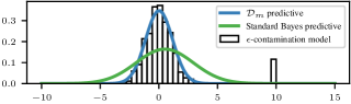
Figure 2: Impact of misspecification in posteriors. The robust ${\mathcal{D}}_{m}$-posterior and non-robust standard Bayes posterior predictive when the data are incorrectly modelled as Gaussian, but follow an $\varepsilon$-contamination model ${\mathbb{P}}=0.95\mathcal{N}(0,1)+0.05\delta_{10}$.

Building a BOCD algorithm based on $\pi^{{\mathcal{D}}_{m}}_{\omega}(\theta|x_{1:T})$ is attractive not only computationally, but also due to its robustness. We prove this robustness formally by using the classical framework of $\varepsilon$-contamination models (see, e.g. Huber, 1981). Given a distribution ${\mathbb{P}}$, we consider its $\varepsilon$-contaminated counterpart ${\mathbb{P}}_{\varepsilon,y}=(1-\varepsilon){\mathbb{P}}+\varepsilon\delta_{y}$, where $\delta_{y}$ is the dirac-measure at some $y\in{\mathcal{X}}$, and $\varepsilon\in[0,1]$. The classical perspective on robustness proceeds by defining a point estimator $E:\mathcal{P}(\mathcal{X})\to\Theta$ that maps from $\mathcal{P}(\mathcal{X})$, the space of distributions on $\mathcal{X}$, to $\Theta$. One then investigates its robustness via $\lim_{\varepsilon\to 0}\frac{1}{\varepsilon}\|E({\mathbb{P}})-E({\mathbb{P}}_{\varepsilon,y})\|_{2}$, which under mild conditions is equivalent to the derivative $\frac{\partial}{\partial\varepsilon}\|E({\mathbb{P}}_{\varepsilon,y})\|_{2}\big{|}_{\varepsilon=0}$. This limit is the so-called influence function. It quantifies the impact of an infinitesimal contamination at $y$ on the estimator, and is a classical tool to measure outlier robustness.

The Bayesian case is slightly more complicated and depicted in Figure 2: we are not concerned by estimators on $\Theta$, but on $\mathcal{P}(\Theta)$. The estimates under study are thus infinite-dimensional objects that vary over $\Theta$. To get a handle on this, we first define an influence function pointwise for each $\theta\in\Theta$. To this end, note that $\widehat{\mathcal{D}}_{m}(\theta)=\mathbb{E}_{X\sim{\mathbb{P}}_{T}}[d_{m}(\theta,X)]$. We can now define the density-valued estimator $\pi^{{\mathcal{D}}_{m}}_{\omega}(\theta|{\mathbb{P}})\propto\pi(\theta)\exp\{-\omega T\mathbb{E}_{X\sim{\mathbb{P}}}[d_{m}(\theta,X)]\}$, noting $\pi^{{\mathcal{D}}_{m}}_{\omega}(\theta|{\mathbb{P}}_{T})=\pi^{{\mathcal{D}}_{m}}_{\omega}(\theta|x_{1:T})$ for ${\mathbb{P}}_{T}=\frac{1}{T}\sum_{t=1}^{T}\delta_{x_{t}}$. Its pointwise posterior influence function (PIF) is rCl PIF(y,θ,P) = ddεπ^D_m_ω(θ—P_ε, y)—_ε=0. Since this is a definition of sensitivity that is local to both $\theta$ and $y$, making a global statement for all of $\pi^{{\mathcal{D}}_{m}}_{\omega}(\theta|x_{1:T})$ requires that we aggregate a notion of sensitivity over both arguments. The easiest way to do this is to investigate $\sup_{\theta\in\Theta,y\in\mathcal{X}}\text{PIF}(y,\theta,{\mathbb{P}}_{T})$. If this double supremum is bounded, we call a posterior globally bias-robust, which means that the impact of contamination on the posterior density is uniformly bounded—both over the parameter space, and the location of said contamination in the data space. This way of studying the robustness of generalised posteriors was pioneered in Ghosh & Basu (2016), and extended by Matsubara et al. (2022b). We build on these advances, and provide a simple condition on $m$ for global bias-robustness of $\pi^{{\mathcal{D}}_{m}}_{\omega}(\theta|x_{1:T})$ in some exponential family models.

Proposition 3.2.

If $p_{\theta}$ is as in (3.2) so that $\eta(\theta)=\theta$ and $\nabla b=0$, and if the prior is a squared exponential as in Proposition 3.1, then $\pi^{{\mathcal{D}}_{m}}_{\omega}(\theta|x_{1:T})$ is globally bias-robust if $m:{\mathcal{X}}\to{\mathbb{R}}^{d\times d}$ is chosen so that $\theta^{\star}\neq 0_{p}$ and

$$\textstyle m_{ij}(x)=\left\{\begin{aligned} \textstyle&\textstyle\dfrac{1}{\sqrt{1+(\nabla r(x)\theta^{\star})_{i}^{2}}}&\textstyle&\textstyle\text{if }i=j,\\ \textstyle&\textstyle 0&\textstyle&\textstyle\text{if }i\neq j.\end{aligned}\right.$$

While $m$ could in principle depend on $\theta$, this would break the conjugacy presented in Proposition 3.1. The above choice of $m$ does not depend on $\theta$, and therefore maintains the computational advantages of $\pi^{{\mathcal{D}}_{m}}_{\omega}(\theta|x_{1:T})$. The result’s conditions are also mild: we can always ensure that $\eta(\theta)=\theta$ by re-parameterising. Similarly, most distributions of interest satisfy $\nabla b=0$. Examples include Gaussians, exponentials, (inverse) Gamma, and Beta distributions. Note also that $m$ is only applicable to models with support $\mathcal{X}={\mathbb{R}}^{d}$, as the expansion in (3.1) is otherwise not valid without additional boundary conditions. However, we prove that the proposed weight matrix $m$ also leads to a well-defined discrepancy measure for various distributions defined on subsets of $\mathcal{X}$, including the Gamma and the exponential distribution (see Section B.5).

3.4 ${\mathcal{D}}_{m}$-BOCD

Using our robust posterior within BOCD is straightforward, as its only appearance is in the posterior predictive via

$$\textstyle p\big{(}x_{t}|x^{(r)}_{t-1}\big{)}=\int_{\Theta}p_{\theta}(x_{t})\pi^{{\mathcal{D}}_{m}}_{\omega}\big{(}\theta|x^{(r)}_{t-1}\big{)}d\theta.$$

If $p_{\theta}$ is a natural exponential family with a squared exponential prior, then $\pi^{{\mathcal{D}}_{m}}_{\omega}(\theta|x^{(r)}_{t-1}))$ is a normal distribution parameterised by inverse covariance matrix $\Sigma_{t-1,r}^{-1}$ and mean $\mu_{t-1,r}$ by virtue of 3.1. This makes the predictive easy to compute—either in closed form or by sampling from $\pi^{{\mathcal{D}}_{m}}_{\omega}$—which is a significant advantage over the $\beta$-BOCD framework. For the latter, the posterior will generally be intractable so that the algorithm relies on variational approximations. Importantly, there is no way to both efficiently and exactly update variational approximations based on $x_{1:t}$ once observation $x_{t+1}$ arrives: one either uses cheap updates that lead to subpar variational approximations of the posterior, or one re-computes the approximation from scratch at the expense of a substantive computational overhead.

In contrast, our approach allows for a cheap and exact update: if we store $\Sigma_{t-1,r}^{-1}$ and $\mu_{t-1,r}$, we can perform the update $\pi^{{\mathcal{D}}_{m}}_{\omega}(\theta|x^{(r)}_{t-1})\mapsto\pi^{{\mathcal{D}}_{m}}_{\omega}(\theta|x^{(r+1)}_{t})$ that adds $x_{t}$ into the parameter posterior of the segment $x^{(r)}_{t-1}$ via

$$\textstyle\Sigma_{t,r+1}^{-1} \textstyle=\Sigma_{t-1,r}^{-1}+2\omega\Lambda(x_{t}),$$

$$\textstyle\mu_{t,r+1} \textstyle=\Sigma_{t,r+1}\left(\Sigma_{t-1,r}^{-1}\mu_{t-1,r}-2\omega\nu(x_{t})\right).$$

If we have access to the un-inverted matrix $\Sigma_{t,r+1}$, all of these operations are basic matrix and vector additions or multiplications that take ${\mathcal{O}}(p^{2}+d^{2})$ operations to execute. While naively computing $\Sigma_{t,r+1}$ from $\Sigma_{t,r+1}^{-1}$ would take ${\mathcal{O}}(p^{3})$ operations, we can apply the Sherman-Morrison formula to the update of $\Sigma_{t,r+1}^{-1}$ to reduce this to ${\mathcal{O}}(p^{2})$, maintaining the overall complexity of ${\mathcal{O}}(p^{2}+d^{2})$. This is also the complexity of standard BOCD with the Gaussian likelihood and conjugate prior (Adams & MacKay, 2007). In CP methods for high-frequency data, both the number of parameters $p$ and the data dimension $d$ are typically small, so that an update of ${\mathcal{O}}(p^{2}+d^{2})$ is attractive.

Run-length pruning.

A naive implementation of ${\mathcal{D}}_{m}$-BOCD would keep a posterior over all possible run-lengths $r_{t}=\{0,1\dots,t-1\}$, but this would lead to an algorithm with overall complexity ${\mathcal{O}}(\sum_{t=1}^{T}t(d^{2}+p^{2}))={\mathcal{O}}(T^{2}(d^{2}+p^{2}))$ for a time series of length $T$. To prevent this, authors have proposed to ‘prune’ the run-length posterior to a constant length (Adams & MacKay, 2007; Fearnhead & Liu, 2007). Here, we follow the most popular strategy (e.g. Adams & MacKay, 2007; Saatçi et al., 2010; Knoblauch & Damoulas, 2018) by keeping only the $k$ most probable run-lengths. For all experiments, we take $k=50$.

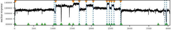
Figure 3: Well-log data. MAP segmentation indicated by blue dashed lines for ${\mathcal{D}}_{m}$-BOCD, ${\color[rgb]{255,127,0}\blacktriangledown}$ for $\beta$-BOCD, and ${\color[rgb]{77,175,74}\blacktriangle}$ for standard BOCD. Standard BOCD mistakenly labels outliers as CPs, while both ${\mathcal{D}}_{m}$-BOCD and $\beta$-BOCD are robust and identify lasting changes.

Choice of $m$

Throughout, we choose $m$ as per Proposition 3.2, as it ensures robustness—even for certain distributions with boundaries (see Section B.5). Regarding $\theta^{\star}$, we found that ${\mathcal{D}}_{m}$-BOCD was not very sensitive to this choice; likely because tuning $\omega$ offsets any sensitivity to it. In all experiments, we thus picked $\theta^{\star}$ as the maximum likelihood estimate computed on the full data set. We note that one known issue with robust CP detection method is that they can experience a latency when it comes to detecting actual CPs. Interestingly, this is not something we observe in our experiments with this choice of $m$ and $\theta^{*}$.

Choice of $\omega$

How to choose $\omega$ is an important question for generalised Bayesian inference, and has more than one answer (Lyddon et al., 2019; Syring & Martin, 2019; Matsubara et al., 2022a; Bochkina, 2022; Wu & Martin, 2023). Previous methods are computationally expensive, asymptotically motivated, and focus on tuning the learning rate to provide asymptotically correct frequentist coverage. As the computational overhead of these methods is substantial and their asymptotic arguments generally do not apply to the CP setting, we pursue a different strategy: we match the uncertainty of the generalised posterior to that of its standard counterpart on the first $t^{\star}$ observations of the data stream. To operationalise this, we choose

$$\textstyle\omega^{\star}=\operatorname*{arg\,min}_{\omega>0}\operatorname{KL}\left(\pi^{{\mathcal{D}}_{m}}_{\omega}(\theta|x_{1:t^{\star}})\|\pi^{\operatorname{B}}(\theta|x_{1:t^{\star}})\right).$$

Computing $\omega^{\star}$ is implemented using automatic differentiation via jax (Bradbury et al., 2018). This is possible even if the standard Bayes posterior $\pi^{\operatorname{B}}$ is intractable, since $\pi^{{\mathcal{D}}_{m}}_{\omega}$ has a conjugacy property (see Proposition 3.1). Since the standard Bayes posterior is reliable in the absence of outliers and heterogeneity, this yields reasonable uncertainty quantification if the degree of misspecification is mild at the beginning of the data stream. Our experiments confirm this: the uncertainty is well-calibrated, both predictively and with regards to the run-length posterior.

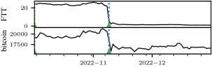
Figure 4: Crypto-crash. MAP segmentation indicated by blue dashed lines for ${\mathcal{D}}_{m}$-BOCD, and by ${\color[rgb]{77,175,74}\blacktriangle}$ for standard BOCD. There are no outliers, so both methods identify the correct CP.

4 Experiments

We investigate ${\mathcal{D}}_{m}$-BOCD empirically in several numerical experiments. In doing so, we highlight its computational and inferential advantages over standard BOCD and $\beta$-BOCD. In all experiments, we choose conjugate priors as in Proposition 3.1, and $m$ and $\omega$ as in Section 3.4. All code and data is publicly available at https://github.com/maltamiranomontero/DSM-bocd.

Computational complexity.

We compare the complexity of the three BOCD methods in different settings and show that ${\mathcal{D}}_{m}$-BOCD is considerably faster than $\beta$-BOCD, even when sampling is needed. Moreover, Figure 5 shows that ${\mathcal{D}}_{m}$ is as fast as standard BOCD when $d=1$ and the predictive posterior is available in closed form. See Section C.1 for details.

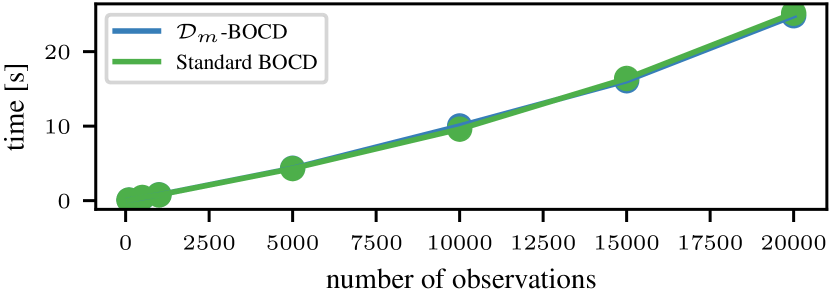
Figure 5: Overall time in seconds versus number of observations. We observe that both methods are equally fast for any number of observations.

Accuracy and detection delay.

We quantify the method’s performance advantage by comparing detection delay and accuracy on artificially generated data with outliers. We generate 600 samples with 2% of outliers and 6 CPs; then, we report the positive predictive value (PPV), true positive rate (TPR), and detection delay. See Section C.3 for the exact expression of the metrics. Table 1 shows that our method detects the same amount of true positives as the standard BOCD while not detecting many false positives, showing the strength of our method. Moreover, the detection delay shows that in spite of being robust to outliers, ${\mathcal{D}}_{m}$-BOCD does not cause any delay in the detection of CP.

Method	PPV	TPR	Delays
${\mathcal{D}}_{m}$-BOCD	0.907$\pm$0.154	0.883$\pm$0.13	1.643$\pm$0.475
Standard BOCD	0.6$\pm$0.128	0.833$\pm$0.149	1.05$\pm$1.545

Table 1: Performance indices-mean and standard deviation-using the positive predictive value (PPV), true positive rate (TPR), and the detection delays over 10 realisations. For PPV and TPR, the nearest to 1, the better. For delays, the lower, the better.

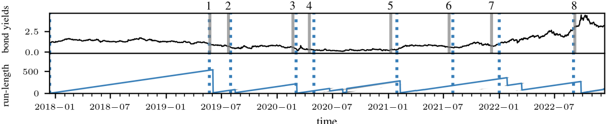
Figure 6: UK’s 10 year government bond yield 2018-2023. The MAP-segmentation resulting from ${\mathcal{D}}_{m}$-BOCD is indicated in dashed blue lines. The bottom panel displays the corresponding run-length posterior, with the most likely run-length marked in blue. A series of political events of national importance closely track the segmentation, and are marked with solid gray lines: 1. Theresa May announces her resignation from her position as prime minister; 2. Boris Johnson sworn in as prime minister; 3. the first Covid case recorded in EU; 4. the first Covid wave in the UK is officially declared; 5. the third Covid wave in the UK is officially declared; 6. the legal limits on social contact removed in UK; 7. Covid ’Plan B’ measures are implemented in UK in response to the spread of the Omicron variant; 8. Liz Truss is sworn in as prime minister.

Twitter flash crash & Cryptocrash.

A robust CP detection algorithm must not to be fooled by outliers while detecting CP correctly. We show that ${\mathcal{D}}_{m}$-BOCD has this capability on two real-world examples: the first is the Dow Jones Industrial Average (DJIA) index every minute on 17/04/2013, the day of the Twitter flash crash. The data is publicly available on FirstRate Data. That day, the Associated Press’ Twitter account was hacked and falsely tweeted that explosions at the White House had injured then-president Barack Obama. In response, the DJIA dropped by 150 points in a matter of seconds before bouncing back. As Figure 1 shows, this is a clear outlier. Modelling the time series with a Gaussian, the plot shows that ${\mathcal{D}}_{m}$-BOCD successfully ignores this blip, while standard BOCD incorrectly labels it as a CP. The second example tracks the average daily value of FTT and Bitcoin between 10/2022 and 12/2022, data which is publicly available on Yahoo finance. FTT was the token issued by FTX, one of the biggest crypto-exchanges before it failed due to a liquidity crisis on November 11th 2022. The ensuing collapse of FTX marked a crash in the value of various crypto-currencies, including Bitcoin. Using a two-dimensional Gaussian distribution for both ${\mathcal{D}}_{m}$-BOCD and standard BOCD, Figure 4 shows that both methods correctly detect the CP. Figure 12 in Appendix C also displays the run-length posteriors, and shows that robustness does not lead to increased CP detection latency.

Well-log.

The well-log data was introduced in Ruanaidh & Fitzgerald (1996), and consists in 4,050 nuclear magnetic resonance measurements recorded while drilling a well. CPs in the sequence correspond to changes in the sediment layers the drill is penetrating. On top of these clear changes, the data contains outliers and contaminants corresponding to more short-term events in geological history—such as flooding, earthquakes, or volcanic activity. When this data set is studied, its outliers have traditionally been removed before CP detection algorithms are run (see e.g. Adams & MacKay, 2007; Ruggieri & Antonellis, 2016; Levy-leduc & Harchaoui, 2008). We leave them in, and Figure 3 shows that this is unproblematic for ${\mathcal{D}}_{m}$-BOCD, but does lead to falsely labelled CPs with BOCD. We also compare the algorithm with $\beta$-BOCD (Knoblauch et al., 2018), and find that the detected changes are almost identical. On a machine with processor Intel i7-7500U 2.7 GHz, and 12GB of RAM, ${\mathcal{D}}_{m}$-BOCD took about 10 times less than $\beta$-BOCD.

Multivariate synthetic data.

In certain settings, ${\mathcal{D}}_{m}$-posteriors are conjugate when standard posteriors are not. An example is a multivariate time series whose dimensions follow different distributions belonging to the exponential family. To this end, we generate 1000 samples from a time series with CPs at $t=250,750$. Conditional on the CPs, the data is generated independently from an exponential in the first dimension and Gaussian distribution in the second dimension. ${\mathcal{D}}_{m}$-BOCD is immediately applicable, and Figure 7 shows that the algorithm functions reliably. We do not compare to BOCD in this setting: for this model, standard Bayesian posteriors would require expensive sampling algorithms or variational approximations to be employed, rendering the algorithm impractical.

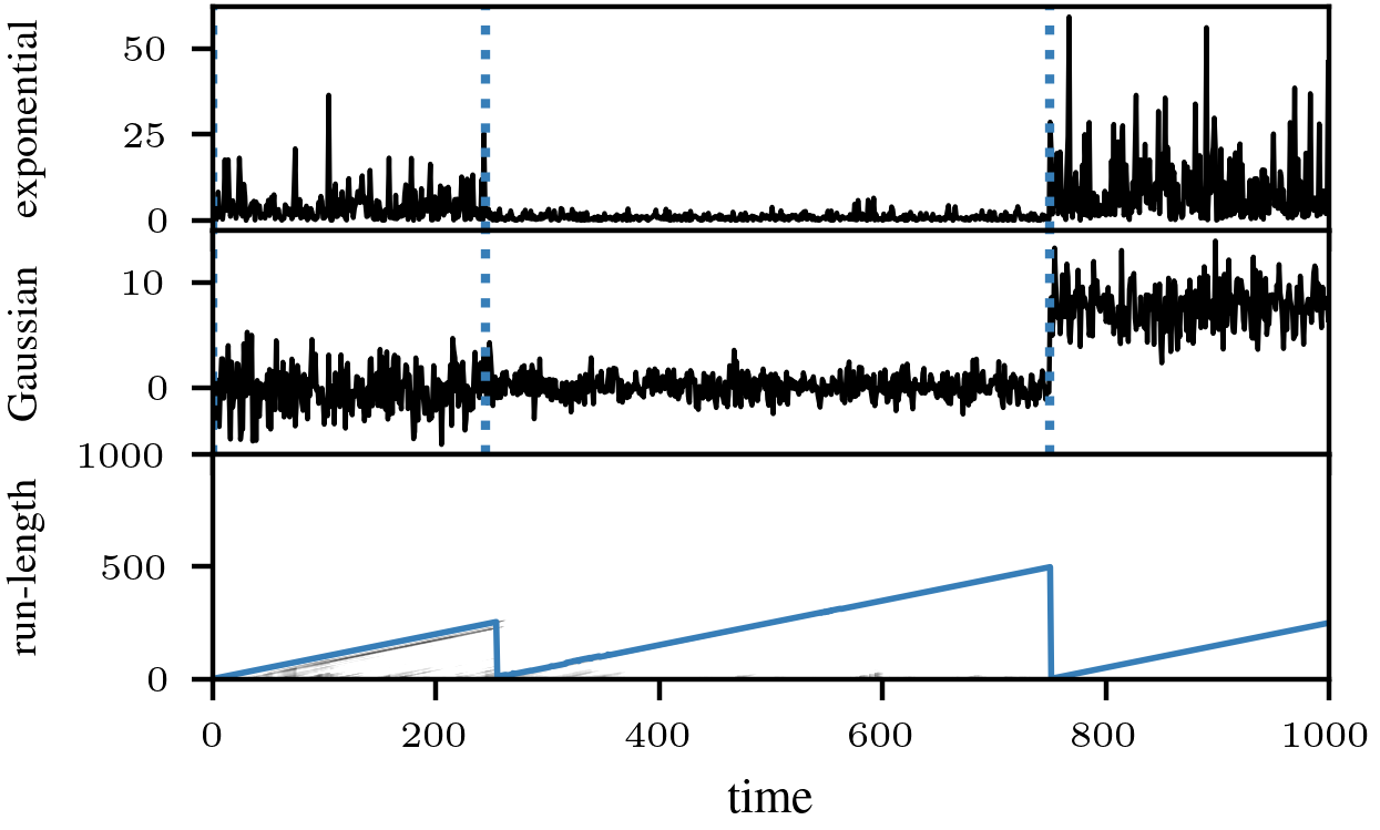
Figure 7: Multivariate synthetic example. A 2-dimensional CP problem. For the chosen model, ${\mathcal{D}}_{m}$-BOCD is computationally efficient, but standard BOCD is computationally infeasible. The MAP segmentation is indicated by dashed blue lines, and the bottom panel shows the run-length distribution, with the most likely value in blue.

UK 10 year government bond yield.

Finally, we run the ${\mathcal{D}}_{m}$-BOCD on the daily yield of 10 year UK government bonds from 2018 to 2022 (see Figure 6). The data is publicly available via the Bank of England database. Since the 10-year yield has been positive throughout history, we model it using the gamma distribution. As shown in Figure 6, we detect changes in the yield curve that correspond to important political events in the UK. This distribution leads to a ${\mathcal{D}}_{m}$-posterior that is a Gaussian truncated at zero. For standard Bayes, a conjugate prior exists, but it leads to a posterior with intractable normalisation constant. Like the multivariate synthetic data example, this constitutes another instance where ${\mathcal{D}}_{m}$-posteriors have better computational properties than standard Bayes.

5 Conclusion

We proposed ${\mathcal{D}}_{m}$-BOCD, a new version of BOCD that is both robust to outliers and scalable. The algorithm relies on a new generalised Bayesian inference scheme constructed with diffusion score-matching. These posteriors have closed form updates for models that are members of the exponential family, and provide robustness by appropriately tuning the diffusion matrix $m$. For $T$ observations, $d$-dimensional data, and $p$ model parameters, the overall run time of the method is ${\mathcal{O}}(T(p^{2}+d^{2}))$, and we demonstrate that it is just as fast as standard BOCD. By showcasing the various computational and inferential benefits of ${\mathcal{D}}_{m}$-BOCD on a range of examples, we demonstrate that it is a powerful and needed addition to the literature. In the future, we will also investigate the applicability of ${\mathcal{D}}_{m}$-BOCD to regression models. This is not trivial: the regression setting changes both the definition of valid score matching losses, as well as how to show their robustness (Xu et al., 2022).

${\mathcal{D}}_{m}$-posteriors also are of independent interest for computational challenges in Bayesian inference: like the generalised posterior in Matsubara et al. (2022b) and Matsubara et al. (2022a), they can be computed even without access to the normalising constant of the likelihood. This suggests that ${\mathcal{D}}_{m}$-posteriors should be studied more broadly as a potential competitor to other Bayesian methods for intractable likelihood problems.

Acknowledgements

We would like to thank Ayush Bharti for feedback on a first draft of this paper. JK was funded by EPSRC grant EP/W005859/1. FXB was supported by the Lloyd’s Register Foundation Programme on Data-Centric Engineering and The Alan Turing Institute under EPSRC grant EP/N510129/1.

Supplementary Materials

In Appendix A, we provide mathematical background. In Appendix B, we present the proofs and derivations of all the theoretical results in our paper, while Appendix C contains additional details regarding our experiments.

Appendix A Background

Let $\nabla=(\partial/\partial x_{1},\ldots,\partial/\partial x_{d})^{\top}$, $f:{\mathcal{X}}\to{\mathbb{R}}^{d}$ and $g:{\mathcal{X}}\to{\mathbb{R}}^{d\times p}$; the divergence operator is define as follows:

$$\textstyle(\nabla\cdot f)(x)=\sum_{i=1}^{d}\dfrac{\partial f_{i}}{\partial x_{i}}(x),\qquad(\nabla\cdot g)_{j}(x)=\sum_{i=1}^{d}\dfrac{\partial g_{ij}}{\partial x_{i}}(x),\quad\forall j\in\{1,...,p\}.$$

Expanding the term $\nabla\cdot mm^{\top}\nabla\log p_{\theta}(x)$ appearing as part of $d_{m}(\theta,x)$, we get

$$\textstyle\nabla\cdot mm^{\top}\nabla\log p_{\theta}(x) \textstyle=\sum_{i=1}^{d}\dfrac{\partial}{\partial x_{i}}(mm^{\top}\nabla\log p_{\theta}(x))_{i}$$

$$\textstyle=\sum_{i=1}^{d}\sum_{j=1}^{d}\dfrac{\partial}{\partial x_{i}}\left((mm^{\top})_{ij}(\nabla\log p_{\theta}(x))_{j}\right)$$

$$\textstyle=\sum_{i=1}^{d}\sum_{j=1}^{d}\left(\dfrac{\partial}{\partial x_{i}}(mm^{\top})_{ij}\right)(\nabla\log p_{\theta}(x))_{j}+\sum_{i=1}^{d}\sum_{j=1}^{d}(mm^{\top})_{ij}\left(\nabla^{2}\log p_{\theta}(x)\right)_{ij}$$

$$\textstyle=\sum_{i=1}^{d}\sum_{j=1}^{d}\left(\dfrac{\partial}{\partial x_{i}}(mm^{\top})_{ij}\right)(\nabla\log p_{\theta}(x))_{j}+\sum_{j=1}^{d}\left(mm^{\top}\nabla^{2}\log p_{\theta}(x)\right)_{jj}$$

$$\textstyle=\sum_{j=1}^{d}\sum_{i=1}^{d}\left(\dfrac{\partial}{\partial x_{i}}(mm^{\top})_{ij}\right)(\nabla\log p_{\theta}(x))_{j}+\operatorname{Tr}\left(mm^{\top}\nabla^{2}\log p_{\theta}(x)\right).$$

Where $\nabla^{2}$ is the Hessian. The expression in the last line is more straightforward to implement in practice and it is therefore the one we use in our code.

The term $\nu(x)$ in Proposition 3.1 contains $(\nabla\cdot(mm^{\top}\nabla r)(x))$. The $j$-th index of this $p$-dimensional vector equals

$$\textstyle(\nabla\cdot(mm^{\top}\nabla r)(x))_{j} \textstyle=\sum_{i=1}^{d}\dfrac{\partial}{\partial x_{i}}(mm^{\top}\nabla r(x))_{ij}.$$

Appendix B Theoretical Results

In this section we present the derivation of the ${\mathcal{D}}_{m}$-posterior, along with the proof of its robustness.

B.1 Proof of Proposition 3.1

In this Subsection we present the proof of the main result of Section 3.2: the conjugacy for exponential family models.

Proof. Let $p_{\theta}$ be an exponential family model. Then $\nabla\log{p_{\theta}}=\nabla r(x)^{\top}\eta(\theta)+\nabla b(x)$, and the DSM estimator has the following form:

$$\textstyle{\widehat{\mathcal{D}}_{m}}(\theta)=\frac{1}{T}\sum_{t=1}^{T}\underbrace{\|m^{\top}(\nabla r(x_{t})\eta(\theta)+\nabla b(x_{t}))\|_{2}^{2}}_{(1)}+2\underbrace{\nabla\cdot(mm^{\top}(\nabla r(x_{t})\eta(\theta)+\nabla b(x_{t})))}_{(2)}.$$

Let $\overset{+C}{=}$ indicate equality up to an additive term that does not depend on $\theta$.

$$\textstyle(1) \textstyle=\eta(\theta)^{\top}\nabla r(x_{t})^{\top}mm^{\top}\nabla r(x_{t})\eta(\theta)+\nabla b(x_{t})^{\top}mm^{\top}\nabla b(x_{t})+2\eta(\theta)^{\top}\nabla r(x_{t})^{\top}mm^{\top}\nabla b(x_{t})$$

$$\textstyle\overset{+C}{=}\eta(\theta)^{\top}\nabla r(x_{t})^{\top}mm^{\top}\nabla r(x_{t})\eta(\theta)+2\eta(\theta)^{\top}\nabla r(x_{t})^{\top}mm^{\top}\nabla b(x_{t}),$$

and

$$\textstyle(2) \textstyle=\nabla\cdot(mm^{\top}\nabla r(x_{t})\eta(\theta))+\nabla\cdot(mm^{\top}\nabla b(x_{t}))$$

$$\textstyle\overset{+C}{=}\nabla\cdot(mm^{\top}\nabla r(x_{t})\eta(\theta))$$

$$\textstyle=\eta(\theta)^{\top}(\nabla\cdot(mm^{\top}\nabla r(x_{t}))).$$

Therefore, ${\widehat{\mathcal{D}}_{m}}(\theta)=\eta(\theta)^{\top}\Lambda_{T}\eta(\theta)+\eta(\theta)^{\top}\nu_{T}$ where

$$\textstyle\Lambda_{T} \textstyle:=\dfrac{1}{T}\sum_{t=1}^{T}\nabla r(x_{t})^{\top}mm^{\top}\nabla r(x_{t}),$$

$$\textstyle\nu_{T} \textstyle:=\dfrac{2}{T}\sum_{t=1}^{T}\nabla r(x_{t})^{\top}mm^{\top}\nabla b(x_{t})+\nabla\cdot(mm^{\top}\nabla r(x_{t})).$$

Now, assuming the prior has a p.d.f. $\pi$, the DSM-Bayes generalised posterior has a p.d.f.

$$\textstyle\pi_{\omega}^{{\mathcal{D}}_{m}}\propto\pi(\theta)\exp{(-\omega T[\eta(\theta)^{\top}\Lambda_{T}\eta(\theta)+\eta(\theta)^{\top}\nu_{T}])}.$$

For $\eta(\theta)=\theta$, and the prior $\pi(\theta)\propto\exp{(-\frac{1}{2}(\theta-\mu)^{\top}\Sigma^{-1}(\theta-\mu))}$, we obtain the generalised posterior by completing the square as follows:

$$\textstyle\pi_{\omega}^{{\mathcal{D}}_{m}}(\theta) \textstyle\propto\exp{(-\frac{1}{2}(\theta-\mu)^{\top}\Sigma^{-1}(\theta-\mu_{T}))}\exp{(-\omega T[\theta^{\top}\Lambda_{T}\theta+\theta^{\top}\nu_{T}])}$$

$$\textstyle=\exp\left(-\dfrac{1}{2}\left(\theta^{\top}\Sigma^{-1}\theta-2\theta^{\top}\Sigma^{-1}\mu+\mu^{\top}\Sigma^{-1}\mu+\theta^{\top}2\omega T\Lambda_{T}\theta+\theta^{\top}2\omega n\nu_{T}\right)\right)$$

$$\textstyle\propto\exp\left(-\dfrac{1}{2}\left(\theta^{\top}(\Sigma^{-1}+2\omega T\Lambda_{T})\theta-2\theta^{\top}(\Sigma^{-1}\mu-\omega T\nu_{T})\right)\right)$$

$$\textstyle\propto\exp{\left(-\frac{1}{2}(\theta-\mu_{T})^{\top}\Sigma_{T}^{-1}(\theta-\mu_{T})\right)},$$

where

$$\textstyle\Sigma_{T}^{-1} \textstyle:=\Sigma^{-1}+2\omega T\Lambda_{T},$$

$$\textstyle\mu_{T} \textstyle:=\Sigma_{T}\left(\Sigma^{-1}\mu-\omega T\nu_{T}\right).$$

$\blacksquare$

B.2 Update Parameters for online DSM-Bayes

In this Section we derive the efficient parameter updates presented in Section 3.4. To do so, we expand the expressions $\Lambda$ and $\nu$ as follows:

$$\textstyle\Lambda_{T+1} \textstyle:=\dfrac{1}{T+1}\sum_{t=1}^{T+1}\nabla r(x_{t})^{\top}mm^{\top}\nabla r(x_{t})$$

$$\textstyle=\dfrac{1}{T+1}\left(\sum_{t=1}^{T}\nabla r(x_{t})^{\top}mm^{\top}\nabla r(x_{t})+\nabla r(x_{T+1})^{\top}mm^{\top}\nabla r(x_{T+1})\right)$$

$$\textstyle=\dfrac{1}{T+1}\left(n\Lambda_{T}+\nabla r(x_{T+1})^{\top}mm^{\top}\nabla r(x_{T+1})\right)$$

$$\textstyle\nu_{T+1} \textstyle:=\dfrac{2}{T+1}\sum_{t=1}^{T+1}\nabla r(x_{t})^{\top}mm^{\top}\nabla b(x_{t})+\nabla\cdot(mm^{\top}\nabla r(x_{t}))$$

$$\textstyle=\dfrac{1}{T+1}\left(T\nu_{T}+2(\nabla r(x_{T+1})^{\top}mm^{\top}\nabla b(x_{T+1})+\nabla\cdot(mm^{\top}\nabla r(x_{T+1}))\right).$$

Now, assuming the prior has the conjugate form of Proposition 3.1, the ${\mathcal{D}}_{m}$-posterior is given by

$$\textstyle\pi_{\omega}^{{\mathcal{D}}_{M}}(\theta)\propto\exp{\left(-\frac{1}{2}(\theta-\mu_{T})^{\top}\Sigma_{T}^{-1}(\theta-\mu_{T})\right)},$$

where

$$\textstyle\Sigma_{T}^{-1} \textstyle:=\Sigma^{-1}+2\omega n\Lambda_{T},$$

$$\textstyle\mu_{T} \textstyle:=\Sigma_{T}\left(\Sigma^{-1}\mu-\omega n\nu_{T}\right).$$

So the parameter updates for $\Sigma_{T}$ and $\mu_{T}$ as $T$ increases are:

$$\textstyle\Sigma_{T+1}^{-1} \textstyle:=\Sigma^{-1}+2\omega(T+1)\Lambda_{T+1}$$

$$\textstyle=\Sigma^{-1}+2\omega\left(n\Lambda_{T}+\nabla t(x_{T+1})^{\top}mm^{\top}\nabla t(x_{T+1})\right)$$

$$\textstyle=\Sigma_{T}^{-1}+2\omega\nabla r(x_{T+1})^{\top}mm^{\top}\nabla r(x_{T+1})$$

$$\textstyle\mu_{T+1} \textstyle:=\Sigma_{T+1}\left(\Sigma^{-1}\mu-\omega(T+1)\nu_{T+1}\right)$$

$$\textstyle=\Sigma_{T+1}\left(\Sigma^{-1}\mu-\omega\left(T\nu_{T}+2(\nabla r(x_{T+1})^{\top}mm^{\top}\nabla b(x_{T+1})+\nabla\cdot(mm^{\top}\nabla r(x_{T+1}))\right)\right)$$

$$\textstyle=\Sigma_{T+1}\left(\Sigma_{T}^{-1}\mu_{T}-2\omega\left(\nabla r(x_{T+1})^{\top}mm^{\top}\nabla b(x_{T+1})+\nabla\cdot(mm^{\top}\nabla r(x_{T+1})\right)\right).$$

obtaining the desired expression.

B.3 Global Bias-Robustness

In this Subsection, we present the theory necessary to prove that the generalized posterior presented in Section 3.1 is global bias-robust conditioned to the choice of $m$.

We first need to review a result from Matsubara et al. (2022a) which states conditions for a discrepancy measure $\mathcal{D}(\theta)$ in order to prove that the corresponding generalised Bayes posterior $\pi_{\omega}^{\mathcal{D}}$ is globally robust to outliers. As in the original results, we will state our findings in terms of distributions ${\mathbb{P}}\in\mathcal{P}(\mathcal{X})$, where $\mathcal{P}(\mathcal{X})$ denotes the set of probability distributions on $\mathcal{X}$. To this end, we will build on the notation introduced in Section 3.3, and write rCl π_ω^D(θ— P)∝π(θ) exp{-ωT ⋅D(θ; P)}    for   D(θ; P) = E_X ∼P[d(θ, X)]. Here, the the discrepancy-based loss $\mathcal{D}(\theta;{\mathbb{P}})=\mathbb{E}_{X\sim{\mathbb{P}}}[d(\theta,X)]$ allows us to recover theoretical posteriors based on averaging some kind of discrepancy $d:\Theta\times\mathcal{X}\to\mathbb{R}$ for any measure $\mathbb{P}$. This makes the results more general and more natural to derive. Note that all derived results apply to the ${\mathcal{D}}_{m}$-posterior computed from data points $x_{1:T}$, as we can recover it by considering $d=d_{m}$, and the corresponding empirical measure ${\mathbb{P}}_{T}=\frac{1}{T}\sum_{t=1}^{T}\delta_{x_{t}}$. In particular, for $d=d_{m}$ we have that $\mathcal{D}(\theta;{\mathbb{P}}_{T})=\widehat{\mathcal{D}}_{m}(\theta)$ so that $\pi_{\omega}^{\mathcal{D}}(\theta|{\mathbb{P}}_{T})=\pi_{\omega}^{\mathcal{D}_{m}}(\theta|x_{1:T})$ as defined in (3.1).

The original work of Matsubara et al. (2022b) constructed a proof of robustness for posteriors that did not depend on an averaged loss $\mathcal{D}(\theta;{\mathbb{P}})=\mathbb{E}_{X\sim{\mathbb{P}}}[d(\theta,X)]$, and so the conditions they derive do not exploit this averaged form. Instead, they showed in Lemma 5 of their paper that global bias-robustness holds if rCl sup_θ∈Θ sup_y∈X —ddεD(θ;P_ε,y)—_ε=0(y,θ,P)—π(θ) & ¡ ∞,    and
∫_Θsup_y∈X —ddεD(θ;P_ε,y)—_ε=0(y,θ,P)—π(θ)dθ ¡ ∞. Clearly, we can simplify this further because our loss is an average. As long as the function $d$ over which the loss is averaged is sufficiently regular, the below result shows that we obtain global bias-robustness.

Proposition B.1.

For each $\theta\in\Theta$. Suppose that $\pi$ is upper bounded over $\Theta$. If there exists a function $\gamma:\Theta\to{\mathbb{R}}$ such that:

1. $\sup_{y\in{\mathcal{X}}}|d(\theta,y)|\leq\gamma(\theta)$ ,

2. $\sup_{\theta\in\Theta}\gamma(\theta)\pi(\theta)<\infty$ , and

3. $\int_{\Theta}\gamma(\theta)\pi(\theta)d\theta<\infty$.

Then the posterior influence function $\operatorname{PIF}(y,\theta,{\mathbb{P}})$ of $\pi_{\omega}^{\mathcal{D}}(\theta|{\mathbb{P}})$ defined in (B.3) is bounded over both $\theta\in\Theta$ and $y\in\mathcal{Y}$, so that the $\pi_{\omega}^{\mathcal{D}}(\theta|{\mathbb{P}})$ is globally robust.

Proof.

As outlined above, we simply have to show that the the above conditions suffice to guarantee (B.3) and (B.3). Rewriting the loss function related to the contamination model would be:

$$\textstyle{\mathcal{D}}(\theta;{\mathbb{P}}_{\varepsilon,y})={\mathbb{E}}_{x\sim{\mathbb{P}}_{\varepsilon,y}}[d(\theta,x)]=(1-\varepsilon){\mathbb{E}}_{x\sim{\mathbb{P}}}[d(\theta,x)]+\varepsilon{\mathbb{E}}_{x\sim\delta_{y}}[d(\theta,x)].$$

Then, differentiating the last expression w.r.t. $\varepsilon$, and evaluating $\varepsilon=0$, we obtain:

$$\textstyle\frac{d}{d\varepsilon}{\mathcal{D}}(\theta;{\mathbb{P}}_{\varepsilon,y})|_{\varepsilon=0}={\mathbb{E}}_{x\sim{\mathbb{P}}}[d(\theta,x)]+{\mathbb{E}}_{x\sim\delta_{y}}[d(\theta,x)]$$

Using Jensen’s inequality, we bound the expression $|\frac{d}{d\varepsilon}{\mathcal{D}}(\theta;{\mathbb{P}}_{\varepsilon,y})|_{\varepsilon=0}|$ as follows:

$$\textstyle|\frac{d}{d\varepsilon}{\mathcal{D}}(\theta;{\mathbb{P}}_{\varepsilon,y})|_{\varepsilon=0}| \textstyle\leq|{\mathbb{E}}_{x\sim\delta_{y}}[d(\theta,x)]|+|{\mathbb{E}}_{x\sim{\mathbb{P}}}[d(\theta,x)]|$$

$$\textstyle\leq{\mathbb{E}}_{x\sim\delta_{y}}[|d(\theta,x)|]+{\mathbb{E}}_{x\sim{\mathbb{P}}}[|d(\theta,x)|]$$

$$\textstyle=|d(\theta,y)|+{\mathbb{E}}_{x\sim{\mathbb{P}}}[|d(\theta,x)|]$$

$$\textstyle\leq|d(\theta,y)|+{\mathbb{E}}_{x\sim{\mathbb{P}}}[\sup_{y\in{\mathcal{X}}}|d(\theta,y)|]$$

$$\textstyle=|d(\theta,y)|+\sup_{y\in{\mathcal{X}}}|d(\theta,y)|,$$

and taking a supremum over $y$ we obtain the bound:

$$\textstyle\sup_{y\in{\mathcal{X}}}|\frac{d}{d\varepsilon}{\mathcal{D}}(\theta;{\mathbb{P}}_{\varepsilon,y})|\leq 2\sup_{y\in{\mathcal{X}}}|d(\theta,y)|\leq 2\gamma(\theta),$$

where the last inequality holds since $\gamma$ fulfil condition 1. Using this bound, we check the two conditions of Matsubara et al. (2022b).

1. $\sup_{\theta\in\Theta}\sup_{y\in{\mathcal{X}}}|\frac{d}{d\varepsilon}{\mathcal{D}}(\theta;{\mathbb{P}}_{\varepsilon,y})|\pi(\theta)\leq\sup_{\theta\in\Theta}2\gamma(\theta)\pi(\theta)<\infty$ , and

2. $\int_{\Theta}\sup_{y\in{\mathcal{X}}}|\frac{d}{d\varepsilon}{\mathcal{D}}(\theta;{\mathbb{P}}_{\varepsilon,y})|\pi(\theta)d\theta\leq\int_{\Theta}2\gamma(\theta)\pi(\theta)d\theta<\infty$,

where the last inequalities hold because $\gamma$ meets conditions 2 and 3. Therefore, by virtue of Matsubara et al. (2022b) the posterior is globally bias-robust. $\blacksquare$

B.4 Proof of Proposition 3.2

In this Subsection we provide the proof of Proposition 3.2. The strategy of the proof is simple: We show that $d=d_{m}$ admits a natural function $\gamma$ that satisfies the conditions of Proposition B.1.

Proof.

From Proposition B.1, it is sufficient to find a function $\gamma$ such that:

$$\textstyle\sup_{y\in{\mathcal{X}}}|\underbrace{\|m^{\top}(y)\nabla\log p_{\theta}(y)\|_{2}^{2}}_{(1)}+2\underbrace{\nabla\cdot m(y)m^{\top}(y)\nabla\log p_{\theta}(y)}_{(2)}|\leq\gamma(\theta).$$

Now, following from the form of $m$ in Proposition 3.2 and the fact that $p_{\theta}$ is an exponential family member as in (3.2), we have:

$$\textstyle(1)=\|m^{\top}(y)\nabla\log p_{\theta}(y)\|_{2}^{2} \textstyle=\sum_{i=1}^{d}(m^{\top}(y)\nabla\log p_{\theta}(y))_{i}^{2}=\sum_{i=1}^{d}\dfrac{(\nabla r(x)\theta)_{i}^{2}}{1+(\nabla r(x)\theta^{\star})_{i}^{2}}\leq\sum_{i=1}^{d}\dfrac{(\nabla r(x)\theta)_{i}^{2}}{(\nabla r(x)\theta^{\star})_{i}^{2}}.$$

Using the fact that $\|x\|_{2}^{2}\leq\|x\|_{1}^{2}\leq d\|x\|_{2}^{2}$ for $x\in{\mathbb{R}}^{d}$, we have:

$$\textstyle\sum_{i=1}^{d}\dfrac{(\nabla r(x)\theta)_{i}^{2}}{(\nabla r(x)\theta^{\star})_{i}^{2}}\leq\sum_{i=1}^{d}\dfrac{p\|\theta\|^{2}_{2}}{\|\theta^{\star}\|^{2}_{2}}=\dfrac{dp\|\theta\|^{2}_{2}}{\|\theta^{\star}\|^{2}_{2}}=:\gamma_{1}(\theta).$$

For the second expression, we have:

$$\textstyle(2)=|\nabla\cdot m(y)m^{\top}(y)\nabla\log p_{\theta}(y)| \textstyle=\left|\sum_{i=1}^{d}\dfrac{\partial}{\partial x_{t}}(m(y)m^{\top}(y)\nabla\log p_{\theta}(y))_{i}\right|$$

$$\textstyle=\left|\sum_{i=1}^{d}\dfrac{\partial}{\partial x_{t}}\left(\dfrac{(\nabla r(x)\theta)_{i}}{1+(\nabla r(x)\theta^{\star})_{i}^{2}}\right)\right|$$

$$\textstyle=\left|\sum_{i=1}^{d}\dfrac{(\nabla^{2}r(x)\theta)_{ii}(1+(\nabla r(x)\theta^{\star})_{i}^{2})-2(\nabla r(x)\theta^{\star})_{i}(\nabla r(x)\theta)_{i}(\nabla^{2}r(x)\theta^{\star})_{ii}}{(1+(\nabla r(x)\theta^{\star})_{i}^{2})^{2}}\right|$$

$$\textstyle\leq\sum_{i=1}^{d}\left|\dfrac{(\nabla^{2}r(x)\theta)_{ii}}{1+(\nabla r(x)\theta^{\star})_{i}^{2})}\right|+2\left|\dfrac{(\nabla r(x)\theta^{\star})_{i}(\nabla r(x)\theta)_{i}(\nabla^{2}r(x)\theta^{\star})_{ii}}{(1+(\nabla r(x)\theta^{\star})_{i}^{2})^{2}}\right|.$$

For most distributions of interest, including Gaussians, exponentials, (inverse) Gamma, and Beta distributions, $\left|\dfrac{(\nabla^{2}r(x)\theta)_{ii}}{1+(\nabla r(x)\theta^{\star})_{i}^{2})}\right|$ is bounded for every $\theta\in\Theta$, then:

$$\textstyle\sum_{i=1}^{d}\left|\dfrac{(\nabla^{2}r(x)\theta)_{ii}}{1+(\nabla r(x)\theta^{\star})_{i}^{2}}\right|+2\left|\dfrac{(\nabla r(x)\theta^{\star})_{i}(\nabla r(x)\theta)_{i}(\nabla^{2}r(x)\theta^{\star})_{ii}}{(1+(\nabla r(x)\theta^{\star})_{i}^{2})^{2}}\right| \textstyle\leq dC(\theta)+2C(\theta)\sum_{i=1}^{d}\left|\dfrac{(\nabla r(x)\theta^{\star})_{i}(\nabla r(x)\theta)_{i}}{(1+(\nabla r(x)\theta^{\star})_{i}^{2})^{2}}\right|$$

$$\textstyle\leq dC(\theta)(1+2d\dfrac{\|\theta\|^{2}_{2}}{\|\theta^{\star}\|^{2}_{2}})=:\gamma_{2}(\theta).$$

Defining $\gamma(\theta):=\gamma_{1}(\theta)+\gamma_{2}(\theta)$ we have :

$$\textstyle\sup_{y\in{\mathcal{X}}}\left|\|m^{\top}(y)\nabla\log p_{\theta}(y)\|_{2}^{2}+2\nabla\cdot m(y)m^{\top}(y)\nabla\log p_{\theta}(y)\right|\leq\gamma(\theta).$$

Now we are in a position to verify conditions (1) and (2) of Proposition B.1. Since $\gamma(\theta)$ is a polynomial function, $\pi(\theta)$ is a squared exponential prior, and the squared exponential has infinitely many moments, it is clear that:

$$\textstyle\sup_{\theta\in\Theta}\pi(\theta)\gamma(\theta) \textstyle<\infty,$$

$$\textstyle\int_{\Theta}\pi(\theta)\gamma(\theta)d\theta \textstyle<\infty,$$

which completes the proof. $\blacksquare$

B.5 Boundary and smoothness conditions

In this subsection, we review the boundary and smoothness conditions discussed in Section 3.1, alongside the DSM extension to more general domains ${\mathcal{X}}$.

The smoothness conditions needed to get the expansion of ${\mathcal{D}}_{m}$ as in Section 3.1 for ${\mathcal{X}}={\mathbb{R}}^{d}$ are the following:

Lemma B.2.

If $p_{\theta}$ is twice-differentiable, and $p_{0}mm^{\top}\nabla\log p_{\theta},\nabla\cdot(p_{0}mm^{\top}\nabla\log p_{\theta})\in L^{1}({\mathbb{R}}^{d})$, then we can rewrite ${\mathcal{D}}_{m}$ as in Section 3.1.

Yu et al. (2019) extended the DSM to densities with non-negative support, i.e. ${\mathcal{X}}={\mathbb{R}}^{d}_{\geq 0}$.

Theorem B.3.

Suppose that $\log p_{0}(x)$ and $m$ are continuously differentiable almost everywhere on ${\mathbb{R}}^{d}_{+}$ and $\log p_{\theta}$ is twice continuously differentiable with respect to $x$ on ${\mathbb{R}}^{d}_{+}$. Furthermore, we assume the boundary condition,

$$\textstyle\lim_{|x^{(i)}|\to\infty}p_{0}(x)m_{ii}^{2}(x)\partial_{i}\log p_{\theta}(x)-\lim_{|x^{(i)}|\to 0+}p_{0}(x)m_{ii}^{2}(x)\partial_{i}\log p_{\theta}(x)=0,\forall i\in\{1,...,d\},$$

where $x_{i}$ is the i-dimension of $x$. Then, we can rewrite ${\mathcal{D}}_{m}$ as in Section 3.1

Later, Liu et al. (2022) extended the DSM to densities with support in a Lipschitz Domain, which, intuitively speaking, are bounded connected open domains whose local boundary is a level set of some Lipschitz function.

Theorem B.4.

Assume ${\mathcal{X}}\subset\mathbb{R}^{d}$ is a Lipschitz domain. Suppose $p_{0},\partial_{i}\log p_{\theta}\in H^{1}({\mathcal{X}})$ and that for any $z\in\partial{{\mathcal{X}}}$ it holds that

$$\textstyle\lim_{x\!\rightarrow z}p_{0}(x)m_{ii}^{2}(x)\partial_{i}\log p_{\theta}(x)v_{i}(z)=0,\forall i\in\{1,...,d\},$$

where $x\rightarrow z$ takes any point sequence converging to $z\in\partial{{\mathcal{X}}}$ into account, $v=(v_{1},...,v_{d})$ is the unit outward normal vector on $\partial{{\mathcal{X}}}$, and $H^{1}({\mathcal{X}})$ is the Sobolev-Hilbert space. Then, we can rewrite ${\mathcal{D}}_{m}$ as in Section 3.1.

The Sobolev-Hilbert space is defined as follows:

$$\textstyle H^{1}({\mathcal{X}})=\big{\{}f\in L^{2}({\mathcal{X}})\,\big{|}\,\|f\|_{L^{2}({\mathcal{X}})}^{2}+\sum_{i=1}^{d}\|D_{i}f\|_{L^{2}({\mathcal{X}})}^{2}<\infty\big{\}},$$

where $D_{i}$ is the weak derivative corresponding to $\partial_{i}$ and $\|f\|_{L^{2}({\mathcal{X}})}=\sqrt{\int_{\mathcal{X}}|f(x)|^{2}dx}$.

Gamma distribution

Let $p_{\theta}$ be a gamma distribution, and ${\mathcal{X}}={\mathbb{R}}_{+}$. Assume $p_{0}$ bounded from above and that $\log p_{0}(x)$ is continuously differentiable almost everywhere on ${\mathbb{R}}_{+}$. Then for $m$ as in Proposition 3.2, we have

$$\textstyle\lim_{|x|\to 0+}p_{0}(x)m^{2}(x)\partial\log p_{\theta}(x) \textstyle=\lim_{|x|\to 0+}p_{0}(x)\dfrac{\nabla r(x)\theta+\nabla b(x)}{1+(\nabla r(x)\theta^{\star})_{i}^{2}}$$

$$\textstyle=\lim_{|x|\to 0+}p_{0}(x)\dfrac{\frac{\theta_{1}}{x}-\theta_{2}}{1+(\frac{\theta_{1}^{\star}}{x}-\theta_{2}^{\star})^{2}}$$

$$\textstyle=\lim_{|x|\to 0+}p_{0}(x)\dfrac{x\theta_{1}-x^{2}\theta_{2}}{x+(\theta_{1}^{\star}-x\theta_{2}^{\star})^{2}}$$

$$\textstyle=0.$$

The last equality holds since $p_{0}$ is bounded. Now, for the second boundary condition:

$$\textstyle\lim_{|x|\to\infty}p_{0}(x)m^{2}(x)\partial\log p_{\theta}(x) \textstyle=\lim_{|x|\to\infty}p_{0}(x)\dfrac{\nabla r(x)\theta+\nabla b(x)}{1+(\nabla r(x)\theta^{\star})_{i}^{2}}=\lim_{|x|\to\infty}p_{0}(x)\dfrac{\frac{\theta_{1}}{x}-\theta_{2}}{1+(\frac{\theta_{1}^{\star}}{x}-\theta_{2}^{\star})^{2}}=0.$$

The last equality holds since $p_{0}$ a density, therefore, $\lim_{|x|\to\infty}p_{0}(x)=0$. Then the $m$ proposed in Proposition 3.2 satisfies the boundary conditions in Theorem B.3 for the gamma distribution.

Exponential distribution

Let $p_{\theta}$ be a exponential distribution, and ${\mathcal{X}}={\mathbb{R}}_{+}$. Assume $p_{0}$ bounded, such that $\log p_{0}(x)$ is continuously differentiable almost everywhere on ${\mathbb{R}}_{+}$. Then for $m$ such as in Proposition 3.2 :

$$\textstyle\lim_{|x|\to 0+}p_{0}(x)m^{2}(x)\partial\log p_{\theta}(x) \textstyle=\lim_{|x|\to 0+}p_{0}(x)\dfrac{\nabla r(x)\theta+\nabla b(x)}{1+(\nabla r(x)\theta^{\star})_{i}^{2}}=\lim_{|x|\to 0+}p_{0}(x)=\dfrac{\theta}{1+\theta^{\star 2}}\lim_{|x|\to 0+}p_{0}(x).$$

The term for the second limit would be similar:

$$\textstyle\lim_{|x|\to\infty}p_{0}(x)m^{2}(x)\partial\log p_{\theta}(x) \textstyle=\dfrac{\theta}{1+\theta^{\star 2}}\lim_{|x|\to\infty}p_{0}(x).$$

Therefore, the expression in Theorem B.3 looks as follows:

$$\textstyle\lim_{|x^{(i)}|\to\infty}p_{0}(x)m_{ii}^{2}(x)\partial_{i}\log p_{\theta}(x)-\lim_{|x^{(i)}|\to 0+}p_{0}(x)m_{ii}^{2}(x)\partial_{i}\log p_{\theta}(x)=\dfrac{\theta}{1+\theta^{\star 2}}\left(\lim_{|x|\to\infty}p_{0}(x)-\lim_{|x|\to 0+}p_{0}(x)\right).$$

Then the $m$ proposed in Proposition 3.2 satisfies the boundary conditions in Theorem B.3 if

$\lim_{|x|\to\infty}p_{0}(x)=\lim_{|x|\to 0+}p_{0}(x)$.

Appendix C Additional Details on Numerical Experiments

In this section we give additional details on the numerical experiments of Section 4. We provide the exact prior and $\omega$ used in each experiment. Moreover, we present an extra numerical experiment to compare the computational complexity of standard BOCD and ${\mathcal{D}}_{m}$-BOCD in Section C.1.

C.1 Computational complexity

The computational complexity of both standard BOCD and ${\mathcal{D}}_{m}$-BOCD is linear in the number of data points. To verify that this theoretical complexity mirrors the practical computational overhead, we generate samples from a Gaussian distribution with 1 CP where the mean varies. We vary the sample size from $T=100$ up to $T=20000$. We fit a Gaussian distribution with the correct variance taken as fixed in both the ${\mathcal{D}}_{m}$-BOCD and the standard BOCD. As shown in Figure 8(a), both methods are equally fast for any number of observations.

Although the computational complexity of ${\mathcal{D}}_{m}$-BOCD is linear in the data, it is quadratic in the dimension of the observations, in particular, is ${\mathcal{O}}(T(p^{2}+d^{2}))$. To observe this in practice, we consider the same settings as before, but now we fix the sample size to $T=100$ and vary the data dimensions from $d=1$ up to $d=500$. Figure 8(b) shows that both methods take practically the same time when $d$ is less than $100$.

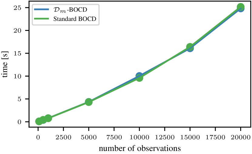
(a) Overall time in seconds versus number of observations. We observe that both methods are equally fast for any number of observations.

(b) Overall time in seconds versus the dimension of the observations. We observe that both methods are practically equally fast when the dimension of the observations is less than $100$.

Figure 8: Comparison between ${\mathcal{D}}_{m}$-BOCD and the standard BOCD. blue line for ${\mathcal{D}}_{m}$-BOCD, and green line for standard BOCD.

The previous setting is where ${\mathcal{D}}_{m}$-BOCD clearly shows its advantage over the $\beta$-BOCD due to its completely closed form, making it nearly equivalent, in terms of computational overhead, to standard BOCD. In more complex settings, the posterior predictive may not be available in closed form; hence, we approximate it by sampling from $\pi_{\omega}^{{\mathcal{D}}_{m}}$. It might not be obvious how this is a significant advantage over the $\beta$-BOCD framework. To demonstrate that ${\mathcal{D}}_{m}$-BOCD is faster than $\beta$-BOCD, we generate samples from a Gaussian distribution with 1 CP, where the mean and the variance change. We vary the sample size from $T=100$ to $T=20000$ and fit a Gaussian distribution in the ${\mathcal{D}}_{m}$-BOCD, $\beta$-BOCD and the standard BOCD. In Figure 9, we observe that although the standard BOCD is faster than ${\mathcal{D}}_{m}$-BOCD, our method is considerably faster than the $\beta$-BOCD for any number of observations.

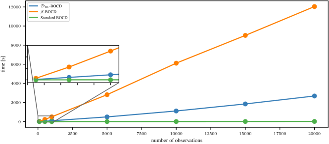
Figure 9: Overall time in seconds versus the number of observations. blue line for ${\mathcal{D}}_{m}$-BOCD, orange line for $\beta$-BOCD, and green line for standard BOCD. We observe that our method is faster than $\beta$-BOCD but is slower than the standard BOCD.

C.2 Varying $m$, $k$, and outliers intensity.

We have demonstrated that our method is insensitive to the scale of the outliers. To do so, we compare the performance of the standard BOCD with the ${\mathcal{D}}_{m}$-BOCD in different contaminated datasets: while everything else stays the same, we scale the contamination points. We generate 600 samples with 6 CPs at $T\in\{200,400\}$, and 3 contaminated point at $T\in\{100,300,500\}$. We contaminate the data by adding (or subtracting) 0, 5, 10, 20, and 40. For the ${\mathcal{D}}_{m}$-BOCD, we choose two different $m$ functions: $m$ as proposed to assure robustness, and $m=I_{d}$. In Figure 10, we observe that both Standard BOCD and ${\mathcal{D}}_{m}$-BOCD with $m=I_{d}$ mistakenly label outliers as CPs, while ${\mathcal{D}}_{m}$-BOCD with $m$ robust is robust and identifies lasting changes.

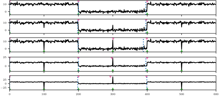
Figure 10: Contamination point scaled by 0, 5, 10, 20, and 40, from top to bottom. MAP segmentation indicated by blue dashed lines for ${\mathcal{D}}_{m}$-BOCD with $m$ robust, ${\color[rgb]{247,129,191}\blacktriangledown}$ for ${\mathcal{D}}_{m}$-BOCD with $m=I_{d}$, and ${\color[rgb]{77,175,74}\blacktriangle}$ for standard BOCD. Both Standard BOCD and ${\mathcal{D}}_{m}$-BOCD with $m=I_{d}$ mistakenly label outliers as CPs, while $\ DSM_{m}$-BOCD with $m$ robust is robust and identifies lasting changes.

Finally, for contamination scaled by 10, we compared the performance and wall-clock time for $k\in\{1,50,600\}$. In Figure 11, we observe that for $k=1$ the method cannot detect any changepoint, while for $k=50$ and $k=600$, the method successfully identifies the changepoints. However, in Table 2 for $k=600$, the method takes 6x more time. As we discussed in the main paper, $k$ is a parameter in all variants of BOCD and will make all algorithms more expensive if increased.

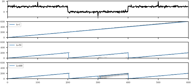
Figure 11: MAP segmentation indicated by blue dashed lines for ${\mathcal{D}}_{m}$-BOCD with $m$ robust. For $k=1$ the method cannot detect any changepoint, while for $k=50$ and $k=600$, the method successfully identifies the changepoints

k	time [s]
1	1
50	38
600	236

Table 2: Wall-clock time for varying $k$

C.3 Accuracy and detection delay

We quantify the method’s performance advantage by comparing detection delay and accuracy on artificially generated data with outliers. In particular, We generate 600 samples with 2% of outliers and 6 CPs; then, we report the positive predictive value (PPV), true positive rate (TPR), and the detection delays. These metrics are given by

$$\text{TPR}=\dfrac{\text{TP}}{\text{TP}+\text{FN}},\quad\quad\text{PPV}=\dfrac{\text{TP}}{\text{TP}+\text{FP}},$$

where TP, FP, and FN are true positives, false positives, and false negatives, respectively. We say the method detects a TP changepoint when the changepoint detected for the method is in a small neighbourhood of the true CP. In order to measure how far the predicted CP is from the true CP, we measure the time difference between both and call it detection delay. For both PPV and TPR, the nearest to 1, the better. For delays, the lower, the better. We run the experiment 10 times, varying the position of the outliers. The following table shows the mean and standard deviation for each metric:

Method	PPV	TPR	Delays
DSM-BOCD	0.907$\pm$0.154	0.883$\pm$0.13	1.643$\pm$0.475
Standard BOCD	0.6$\pm$0.128	0.833$\pm$0.149	1.05$\pm$1.545

Table 3: Performance indices-mean and standard deviation-using the positive predictive value (PPV), true positive rate (TPR), and the detection delays over 10 realisations. For PPV and TPR, the nearest to 1, the better. For delays, the lower, the better.

In Table 3, we observe ${\mathcal{D}}_{m}$-BOCD has a significantly better performance with respect to PPV, meaning that the rate of false positives is lower than standard BOCD. This is a consequence of the robustness of our method. Moreover, we see a similar result concerning TPR, which measures the amount of changepoint not detected for the methods. Overall, this means that our method detects the same amount of TP as the standard BOCD while not detecting many FP, showing the strength of our method. Lastly, the detection delay shows that in spite of being robust to outliers, ${\mathcal{D}}_{m}$-BOCD does not cause any delay in the detection of CP.

C.4 Twitter flash crash & Cryptocrash

In the Twitter flash crash experiment, we model the data with a Gaussian distribution, modelling its natural parameters. For ${\mathcal{D}}_{m}$-BOCD, we use a conjugate squared exponential prior r with parameters $\mu=(0,1)^{\top}$, and $\Sigma$ a diagonal matrix so that $\operatorname{diag}(\Sigma)=(10,1)$ for the natural parameters of said Gaussian. For standard BOCD, we use a Normal-inverse gamma prior with parameters $\mu_{0}=0$, $\nu=1$, $\alpha=2$ and $\beta=10$. We use the first 50 observations to select $\omega$ as in Section 3.4, with an obtained value of $\omega^{\star}\approx 0.0001$

In the Cryptocrash experiment, we model the data with a multivariate Gaussian distribution modelling its natural parameters, and use conjugate squared exponential prior with parameters $\mu=(0,1,0,1)^{\top}$, and $\Sigma$ diagonal matrix such that $\operatorname{diag}(\Sigma)=(2,1,2,1)$ for the ${\mathcal{D}}_{m}$-BOCD. For standard BOCD, we model mean and variance instead, and use a normal-inverse-Wishart prior with parameters $\nu=0,\,\kappa=1,\,\mu=(0,0)$ and $\Psi$ diagonal matrix such that $\operatorname{diag}(\Psi)=(1,1)$. we manually fix $\omega=0.01$. Figure 12 shows the run-length posteriors and the Maximum A Posteriori (MAP) segmentations produced by each method. Since the most likely run-lengths are virtually identical, the below plot also shows that in spite of being robust to outliers, ${\mathcal{D}}_{m}$-BOCD does not cause any delay in the detection of CPs.

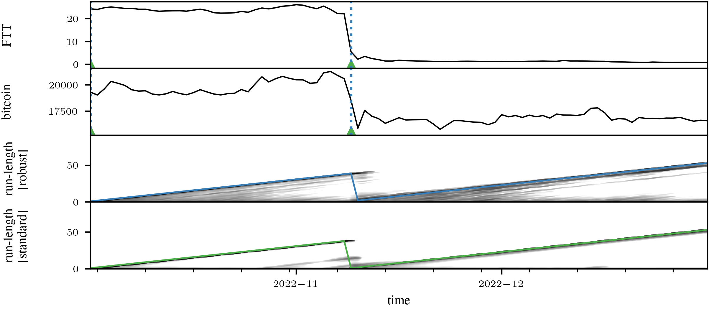
Figure 12: Maximum a posteriori (MAP) segmentation. In blue ${\mathcal{D}}$-BOCD segmentation using dashed lines. In green Standard BOCD segmentation using ${\color[rgb]{77,175,74}\blacktriangle}$ marks. In addition we plot the run-length posteriors of robust ${\mathcal{D}}_{m}$-BOCD algorithm with most likely run-length in blue and of standard BOCD in green. We observe that robustness does not lead to increased CP detection latency: both methods detect the CP at the same time.

C.5 Well-log

We model the data with a Gaussian distribution, modelling its natural parameters and using a conjugate squared exponential prior with parameters $\mu=(0,10)^{\top}$, and $\Sigma$ diagonal matrix such that $\operatorname{diag}(\Sigma)=(100,100)$. Figure 13 shows the run-length and the segmentation of each method. We use the first 200 observations to select $\omega$ as in Section 3.4, with an obtained value of $\omega^{\star}\approx 0.0004$

C.6 Multivariate synthetic data

We generate 1000 samples from a time series with CPs at t = 250, 750. Conditional on the CPs, the data is generated independently from an exponential in the first a and Gaussian distribution in the second dimension. Since both dimensions are exponential family members, their joint distribution is too. On the natural parameters of this joint distribution, we place a conjugate squared exponential prior with parameters $\mu=(1,0,0.5)^{\top}$, and $\Sigma$ diagonal matrix such that $\operatorname{diag}(\Sigma)=(1,1,0.2)$. As we do not compare against BOCD on this data set, we simply fix $\omega^{\star}=0.15$.

C.7 UK 10 year government bond yield

We model the data with a Gamma distribution and use a conjugate squared exponential prior with parameters $\mu=(0,1)^{\top}$, and $\Sigma$ diagonal matrix such that $\operatorname{diag}(\Sigma)=(50,3)$ on its natural parameters. We use the first 100 observations to select $\omega$ as in 3.4. The obtained value is $\omega^{\star}\approx 0.05$.

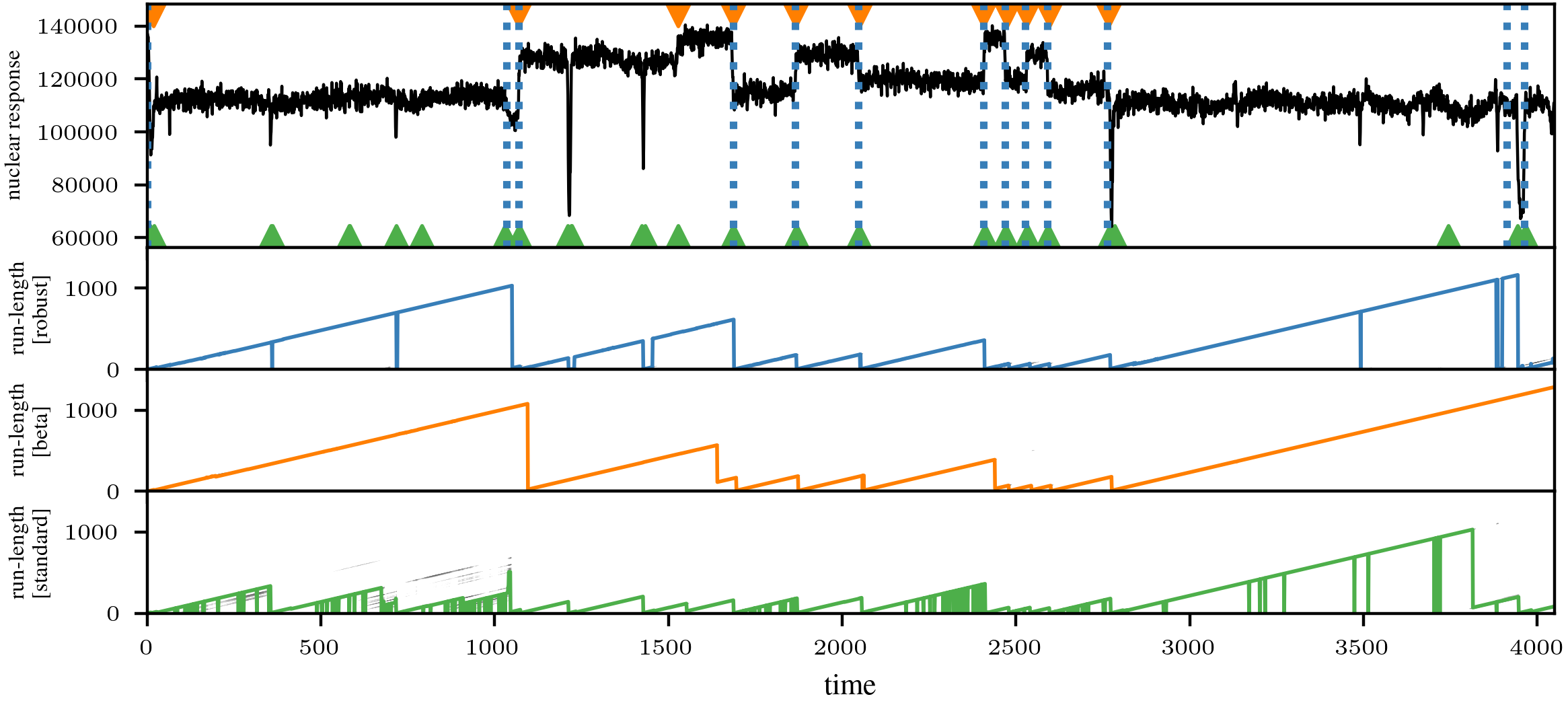
Figure 13: AP segmentation for the well-log indicated by blue dashed lines for ${\mathcal{D}}_{m}$-BOCD, ${\color[rgb]{255,127,0}\blacktriangledown}$ for $\beta$-BOCD, and ${\color[rgb]{77,175,74}\blacktriangle}$ for standard BOCD. In addition we plot the run-length posteriors of robust ${\mathcal{D}}_{m}$-BOCD algorithm with most likely run-length in blue, $\beta$-BOCD in orange, and of standard BOCD in green. We observe that our method is more robust to outliers than the standard BOCD, but is more sensitive than $\beta$-BOCD.

References

- Adams & MacKay (2007) Adams, R. P. and MacKay, D. J. Bayesian online changepoint detection. arXiv:0710.3742, 2007.
- Agudelo-España et al. (2020) Agudelo-España, D., Gomez-Gonzalez, S., Bauer, S., Schölkopf, B., and Peters, J. Bayesian online prediction of change points. In Conference on Uncertainty in Artificial Intelligence, pp. 320–329, 2020.
- Anastasiou et al. (2023) Anastasiou, A., Barp, A., Briol, F.-X., Ebner, B., Gaunt, R. E., Ghaderinezhad, F., Gorham, J., Gretton, A., Ley, C., Liu, Q., Mackey, L., Oates, C. J., Reinert, G., and Swan, Y. Stein’s method meets computational statistics: A review of some recent developments. Statistical Science, 38:120–139, 2023.
- Barp et al. (2019) Barp, A., Briol, F.-X., Duncan, A., Girolami, M., and Mackey, L. Minimum Stein discrepancy estimators. In Advances in Neural Information Processing Systems, pp. 12964–12976, 2019.
- Barry & Hartigan (1993) Barry, D. and Hartigan, J. A. A Bayesian analysis for change point problems. Journal of the American Statistical Association, 88(421):309–319, 1993.
- Basu et al. (1998) Basu, A., Harris, I. R., Hjort, N. L., and Jones, M. Robust and efficient estimation by minimising a density power divergence. Biometrika, 85(3):549–559, 1998.
- Bissiri et al. (2016) Bissiri, P. G., Holmes, C. C., and Walker, S. G. A general framework for updating belief distributions. Journal of the Royal Statistical Society: Series B (Statistical Methodology), 78(5):1103–1130, 2016.
- Bochkina (2022) Bochkina, N. Bernstein-von Mises theorem and misspecified models: a review. arXiv:2204.13614, 2022.
- Boustati et al. (2020) Boustati, A., Akyildiz, O. D., Damoulas, T., and Johansen, A. Generalised Bayesian filtering via sequential Monte Carlo. In Advances in Neural Information Processing Systems, pp. 418–429, 2020.
- Bradbury et al. (2018) Bradbury, J., Frostig, R., Hawkins, P., Johnson, M. J., Leary, C., Maclaurin, D., Necula, G., Paszke, A., VanderPlas, J., Wanderman-Milne, S., and Zhang, Q. JAX: composable transformations of Python+NumPy programs, 2018. URL http://github.com/google/jax.
- Chérief-Abdellatif & Alquier (2020) Chérief-Abdellatif, B.-E. and Alquier, P. MMD-Bayes: Robust Bayesian estimation via maximum mean discrepancy. In Symposium on Advances in Approximate Bayesian Inference, 2020.
- Chernozhukov & Hong (2003) Chernozhukov, V. and Hong, H. An MCMC approach to classical estimation. Journal of Econometrics, 115(2):293–346, 2003.
- Chib (1998) Chib, S. Estimation and comparison of multiple change-point models. Journal of Econometrics, 86(2):221–241, 1998.
- Dawid & Musio (2015) Dawid, A. P. and Musio, M. Bayesian model selection based on proper scoring rules. Bayesian Analysis, 10(2):479–499, 2015.
- Dellaporta et al. (2022) Dellaporta, C., Knoblauch, J., Damoulas, T., and Briol, F.-X. Robust Bayesian inference for simulator-based models via the MMD posterior bootstrap. In International Conference on Artificial Intelligence and Statistics, pp. 943–970, 2022.
- Fearnhead (2006) Fearnhead, P. Exact and efficient Bayesian inference for multiple changepoint problems. Statistics and Computing, 16(2):203–213, 2006.
- Fearnhead & Liu (2007) Fearnhead, P. and Liu, Z. On-line inference for multiple changepoint problems. Journal of the Royal Statistical Society: Series B (Statistical Methodology), 69(4):589–605, 2007.
- Fong et al. (2021) Fong, E., Holmes, C., and Walker, S. G. Martingale posterior distributions. arXiv:2103.15671, 2021.
- Futami et al. (2018) Futami, F., Sato, I., and Sugiyama, M. Variational inference based on robust divergences. In International Conference on Artificial Intelligence and Statistics, pp. 813–822, 2018.
- Ghosh & Basu (2016) Ghosh, A. and Basu, A. Robust Bayes estimation using the density power divergence. Annals of the Institute of Statistical Mathematics, 68(2):413–437, 2016.
- Giummolè et al. (2019) Giummolè, F., Mameli, V., Ruli, E., and Ventura, L. Objective Bayesian inference with proper scoring rules. TEST, 28(3):728–755, 2019.
- Grünwald (2012) Grünwald, P. The safe Bayesian. In International Conference on Algorithmic Learning Theory, pp. 169–183, 2012.
- Gundersen et al. (2021) Gundersen, G. W., Cai, D., Zhou, C., Engelhardt, B. E., and Adams, R. P. Active multi-fidelity Bayesian online changepoint detection. In Uncertainty in Artificial Intelligence, pp. 1916–1926, 2021.
- Hallgren et al. (2022) Hallgren, K. L., Heard, N. A., and Adams, N. M. Changepoint detection in non-exchangeable data. Statistics and Computing, 32(6):1–19, 2022.
- Holmes & Walker (2017) Holmes, C. C. and Walker, S. G. Assigning a value to a power likelihood in a general Bayesian model. Biometrika, 104(2):497–503, 2017.
- Hooker & Vidyashankar (2014) Hooker, G. and Vidyashankar, A. Bayesian model robustness via disparities. TEST, 23(3):556–584, 2014.
- Huber (1981) Huber, P. J. Robust statistics. Wiley Series in Probability and Mathematical Statistics, 1981.
- Hyvärinen (2006) Hyvärinen, A. Estimation of non-normalized statistical models by score matching. Journal of Machine Learning Research, 6:695–708, 2006.
- Hyvärinen (2007) Hyvärinen, A. Some extensions of score matching. Computational Statistics and Data Analysis, 51(5):2499–2512, 2007.
- Itoh & Kurths (2010) Itoh, N. and Kurths, J. Change-point detection of climate time series by nonparametric method. In Proceedings of the World Congress on Engineering and Computer Science, volume 1, pp. 445–448, 2010.
- Jewson & Rossell (2022) Jewson, J. and Rossell, D. General Bayesian loss function selection and the use of improper models. Journal of the Royal Statistical Society Series B: Statistical Methodology, 84(5):1640–1665, 2022.
- Jewson et al. (2018) Jewson, J., Smith, J. Q., and Holmes, C. Principled Bayesian minimum divergence inference. Entropy, 20(6):442, 2018.
- Kawahara & Sugiyama (2009) Kawahara, Y. and Sugiyama, M. Change-point detection in time-series data by direct density-ratio estimation. In Proceedings of the 2009 SIAM International Conference on Data Mining, pp. 389–400. SIAM, 2009.
- Kim et al. (2022) Kim, K., Park, J. H., Lee, M., and Song, J. W. Unsupervised change point detection and trend prediction for financial time-series using a new CUSUM-based approach. IEEE Access, 10:34690–34705, 2022.
- Knoblauch (2019) Knoblauch, J. Robust deep Gaussian processes. arXiv:1904.02303, 2019.
- Knoblauch & Damoulas (2018) Knoblauch, J. and Damoulas, T. Spatio-temporal Bayesian on-line changepoint detection with model selection. In International Conference on Machine Learning, pp. 2718–2727, 2018.
- Knoblauch et al. (2018) Knoblauch, J., Jewson, J. E., and Damoulas, T. Doubly robust Bayesian inference for non-stationary streaming data with -divergences. In Advances in Neural Information Processing Systems, 2018.
- Knoblauch et al. (2022) Knoblauch, J., Jewson, J., and Damoulas, T. An optimization-centric view on Bayes’ rule: Reviewing and generalizing variational inference. Journal of Machine Learning Research, 23(132):1–109, 2022.
- Kummerfeld & Danks (2013) Kummerfeld, E. and Danks, D. Tracking time-varying graphical structure. Advances in Neural Information Processing Systems, 26, 2013.
- Legramanti et al. (2022) Legramanti, S., Durante, D., and Alquier, P. Concentration and robustness of discrepancy-based ABC via Rademacher complexity. arXiv:2206.06991, 2022.
- Levy-leduc & Harchaoui (2008) Levy-leduc, C. and Harchaoui, Z. Catching change-points with lasso. In Advances in Neural Information Processing Systems, pp. 617–624, 2008.
- Liu et al. (2022) Liu, S., Kanamori, T., and Williams, D. J. Estimating density models with truncation boundaries using score matching. Journal of Machine Learning Research, 23(186):1–38, 2022.
- Lyddon et al. (2019) Lyddon, S. P., Holmes, C. C., and Walker, S. G. General Bayesian updating and the loss-likelihood bootstrap. Biometrika, 106(2):465–478, 2019.
- Lyu (2009) Lyu, S. Interpretation and generalization of score matching. In Uncertainty in Artificial Intelligence, pp. 359–366, 2009.
- Mardia et al. (2016) Mardia, K. V., Kent, J. T., and Laha, A. K. Score matching estimators for directional distributions. arXiv:1604.08470, 2016.
- Martin & Syring (2022) Martin, R. and Syring, N. Direct Gibbs posterior inference on risk minimizers: Construction, concentration, and calibration. Handbook of Statistics, 2022.
- Matsubara et al. (2022a) Matsubara, T., Knoblauch, J., Briol, F.-X., Oates, C., et al. Generalised Bayesian inference for discrete intractable likelihood. arXiv:2206.08420, 2022a.
- Matsubara et al. (2022b) Matsubara, T., Knoblauch, J., Briol, F.-X., and Oates, C. J. Robust generalised Bayesian inference for intractable likelihoods. Journal of the Royal Statistical Society: Series B (Statistical Methodology), 84(3):997–1022, 2022b.
- Pacchiardi & Dutta (2021) Pacchiardi, L. and Dutta, R. Generalized Bayesian likelihood-free inference using scoring rules estimators. arXiv:2104.03889, 2021.
- Page (1954) Page, E. S. Continuous inspection schemes. Biometrika, 41(1/2):100–115, 1954.
- Parry et al. (2012) Parry, M., Dawid, A. P., and Lauritzen, S. Proper local scoring rules. Annals of Statistics, 40(1):561–592, 2012.
- Reeves et al. (2007) Reeves, J., Chen, J., Wang, X. L., Lund, R., and Lu, Q. Q. A review and comparison of changepoint detection techniques for climate data. Journal of Applied Meteorology and Climatology, 46(6):900–915, 2007.
- Ruanaidh & Fitzgerald (1996) Ruanaidh, J. J. O. and Fitzgerald, W. J. Numerical Bayesian methods applied to signal processing. Springer Science & Business Media, 1996.
- Ruggieri & Antonellis (2016) Ruggieri, E. and Antonellis, M. An exact approach to Bayesian sequential change point detection. Computational Statistics & Data Analysis, 97:71–86, 2016.
- Saatçi et al. (2010) Saatçi, Y., Turner, R. D., and Rasmussen, C. E. Gaussian process change point models. In International Conference on Machine Learning, 2010.
- Scealy & Wood (2022) Scealy, J. L. and Wood, A. T. A. Score matching for compositional distributions. Journal of the American Statistical Association, to appear, 2022.
- Schmon et al. (2020) Schmon, S. M., Cannon, P. W., and Knoblauch, J. Generalized posteriors in approximate Bayesian computation. In Symposium on Advances in Approximate Bayesian Inference, 2020.
- Shao et al. (2019) Shao, S., Jacob, P. E., Ding, J., and Tarokh, V. Bayesian model comparison with the Hyvarinen score: computation and consistency. Journal of the American Statistical Association, 114(528):1826–1837, 2019.
- Song & Ermon (2019) Song, Y. and Ermon, S. Generative modeling by estimating gradients of the data distribution. Neural Information Processing Systems, 32, 2019.
- Sriperumbudur et al. (2017) Sriperumbudur, B. K., Fukumizu, K., Gretton, A., and Hyvarinen, A. Density estimation in infinite dimensional exponential families. Journal of Machine Learning Research, 18(57):1–59, 2017.
- Stival et al. (2022) Stival, M., Bernardi, M., and Dellaportas, P. Doubly-online changepoint detection for monitoring health status during sports activities. arXiv:2206.11578, 2022.
- Syring & Martin (2019) Syring, N. and Martin, R. Calibrating general posterior credible regions. Biometrika, 106(2):479–486, 2019.
- Turner et al. (2013) Turner, R. D., Bottone, S., and Stanek, C. J. Online variational approximations to non-exponential family change point models: with application to radar tracking. In Advances in Neural Information Processing Systems, 2013.
- Vincent (2011) Vincent, P. A connection between score matching and denoising autoencoders. Neural Computation, 1674:1661–1674, 2011.
- Wilson et al. (2010) Wilson, R. C., Nassar, M. R., and Gold, J. I. Bayesian on-line learning of the hazard rate in change-point problems. Neural Computation, 22(9):2452–2476, 2010.
- Wu & Martin (2023) Wu, P.-S. and Martin, R. A comparison of learning rate selection methods in generalized Bayesian inference. Bayesian Analysis, 18(1):105–132, 2023.
- Wu et al. (2023) Wu, S., Diao, E., Banerjee, T., Ding, J., and Tarokh, V. Quickest change detection for unnormalized statistical models. arXiv:2302.00250, 2023.
- Xu et al. (2022) Xu, J., Scealy, J. L., Wood, A. T., and Zou, T. Generalized score matching for regression. arXiv:2203.09864, 2022.
- Yang et al. (2006) Yang, P., Dumont, G., and Ansermino, J. M. Adaptive change detection in heart rate trend monitoring in anesthetized children. IEEE Transactions on Biomedical Engineering, 53(11):2211–2219, 2006.
- Yu et al. (2018) Yu, S., Drton, M., and Shojaie, A. Graphical models for non-negative data using generalized score matching. In International Conference on Artificial Intelligence and Statistics, pp. 1781–1790, 2018.
- Yu et al. (2019) Yu, S., Drton, M., and Shojaie, A. Generalized score matching for non-negative data. Journal of Machine Learning Research, 20:1–70, 2019.
- Yu et al. (2022) Yu, S., Drton, M., and Shojaie, A. Generalized score matching for general domains. Information and Inference, 11(2):739–780, 2022.
- Zellner (1988) Zellner, A. Optimal information processing and Bayes’s theorem. The American Statistician, 42(4):278–280, 1988.
- Zhai et al. (2016) Zhai, S., Cheng, Y., Lu, W., and Zhang, Z. Deep structured energy based models for anomaly detection. In International Conference on Machine Learning, volume 3, pp. 1742–1751, 2016.
- Zhang et al. (2022) Zhang, M., Key, O., Hayes, P., Barber, D., Paige, B., and Briol, F.-X. Towards healing the blindness of score matching. NeurIPS 2022 workshop on score-based methods, arXiv:2209.07396, 2022.