Scaling Goal-based Exploration via Pruning Proto-goals

Abstract

One of the gnarliest challenges in reinforcement learning (RL) is exploration that scales to vast domains, where novelty-, or coverage-seeking behaviour falls short. Goal-directed, purposeful behaviours are able to overcome this, but rely on a good goal space. The core challenge in goal discovery is finding the right balance between generality (not hand-crafted) and tractability (useful, not too many). Our approach explicitly seeks the middle ground, enabling the human designer to specify a vast but meaningful proto-goal space, and an autonomous discovery process to refine this to a narrower space of controllable, reachable, novel, and relevant goals. The effectiveness of goal-conditioned exploration with the latter is then demonstrated in three challenging environments.

1 Introduction

Exploration is widely recognised as a core challenge in RL. It is most acutely felt when scaling to vast domains, where classical novelty-seeking methods are insufficient (Taiga et al., 2020) because there are simply too many things to observe, do, and learn about; and the agent’s lifetime is far too short to approach exhaustive coverage (Sutton et al., 2022).

Abstraction can overcome this issue (Gershman, 2017; Konidaris, 2019): by learning about goal-directed, purposeful behaviours (and how to combine them), the RL agent can ignore irrelevant details, and effectively traverse the state space. Goal-conditioned RL is one natural formalism of abstraction, and especially appealing when the agent can learn to generalise across goals (Schaul et al., 2015).

The effectiveness of goal-conditioned agents directly depends on the size and quality of the goal space (Section 3). If it is too large, such as treating all encountered states as goals (Andrychowicz et al., 2017), most of the abstraction benefits vanish. On the other extreme, hand-crafting a small number of useful goals (Barreto et al., 2019) limits the generality of the method. The answer to this conundrum is to adaptively expand or refine the goal space based on experience, also known as the discovery problem, allowing for a more autonomous agent that can be both general and scalable.

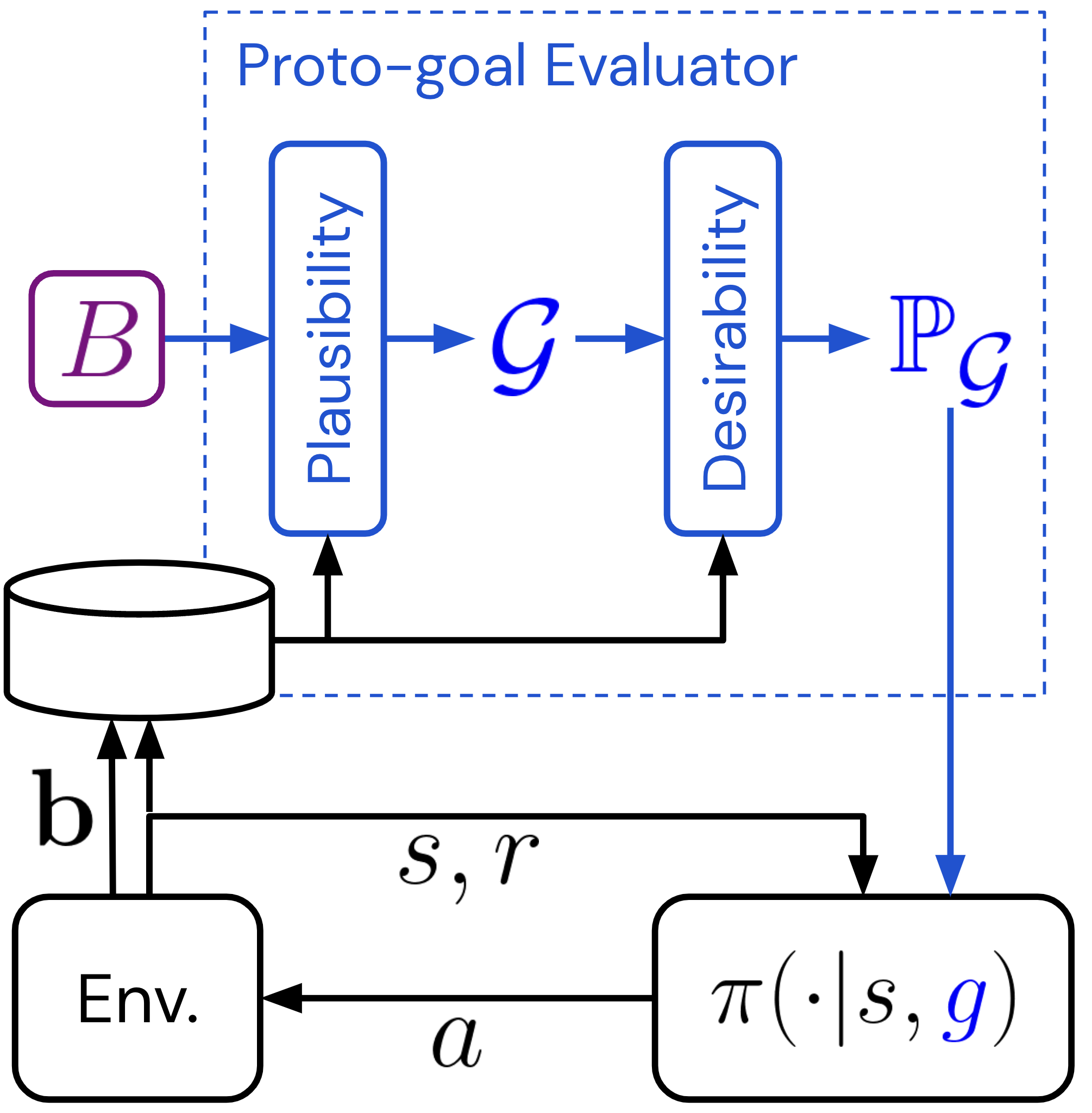
Figure 1: Proto-goal RL: a goal-conditioned RL agent’s policy $\pi$ acts with goals $g$ obtained from its Proto-goal Evaluator (PGE, blue). The PGE refines a cheaply defined proto-goal space ($B$, violet) into a smaller set of plausible goals $\mathcal{G}$, using observed transition data $(s,a,r,s^{\prime})$ that includes information about encountered proto-goals ($\mathbf{b}$). It further endows $\mathcal{G}$ with a distribution $\mathbb{P}_{\mathcal{G}}$, based on goal desirability, from which $g$ is then sampled.

Taking a step towards this ultimate aim, we propose a framework with two elements. First, a proto-goal space (Section 3), which can be cheaply designed to be meaningful for the domain at hand, e.g., by pointing out the most salient part of an observation using domain knowledge (Chentanez et al., 2004). What makes defining a proto-goal space much easier than defining a goal space is its leniency: it can remain (combinatorially) large and unrefined, with many uninteresting or useless proto-goals. Second, an adaptive function mapping this space to a compact set of useful goals, called a Proto-goal Evaluator (PGE, Section 4). The PGE may employ multiple criteria of usefulness, such as controllability, novelty, reachability, learning progress, or reward-relevance. Finally we address pragmatic concerns on how to integrate these elements into a large-scale goal-conditioned RL agent (Section 5), and show it can produce a qualitative leap in performance in otherwise intractable exploration domains (Section 6).

2 Background and Related Work

We consider problems modeled as Markov Decision Processes (MDPs) $\mathcal{M}=(\mathcal{S},\mathcal{A},\mathcal{R},\mathcal{T},\gamma)$, where $\mathcal{S}$ is the state space, $\mathcal{A}$ is the action space, $\mathcal{R}$ is the reward function, $\mathcal{T}$ is the transition function and $\gamma$ is the discount factor. The aim of the agent is to learn a policy that maximises the sum of expected rewards (Sutton and Barto, 2018).

Exploration in RL.

Many RL systems use dithering strategies for exploration (e.g., $\epsilon$-greedy, softmax, action-noise (Lillicrap et al., 2016) and parameter noise (Fortunato et al., 2018; Plappert et al., 2018)). Among those that address deep exploration, the majority of research (Taiga et al., 2020) has focused on count-based exploration (Strehl and Littman, 2008; Bellemare et al., 2016), minimizing model prediction error (Pathak et al., 2017; Burda et al., 2019a, b), or picking actions to reduce uncertainty (Osband et al., 2016, 2018) over the state space. These strategies try to eventually learn about all states, which might not be a scalable strategy when the world is a lot bigger than the agent (Sutton et al., 2022). We build on the relatively under-studied family of exploration methods that maximize the agent’s learning progress (Schmidhuber, 1991; Kaplan and Oudeyer, 2004).

General Value Functions.

Rather than being limited to predicting and maximizing a single reward (as in vanilla RL), General Value Functions (GVFs) (Sutton et al., 2011) predict (and sometimes control (Jaderberg et al., 2017)) “cumulants” that can be constructed out of the agent’s sensorimotor stream. The discounted sum of these cumulants are GVFs and can serve as the basis of representing rich knowledge about the world (Schaul and Ring, 2013; Veeriah et al., 2019).

Goal-conditioned RL.

When the space of cumulants is limited to goals, GVFs reduce to goal-conditioned value functions that are often represented using Universal Value Function Approximators (UVFAs) (Schaul et al., 2015). Hindsight Experience Replay (HER) is a popular way of learning UVFAs in a sample-efficient way (Andrychowicz et al., 2017). The two most common approaches is to assume that a set of goals is given, or to treats all observations as potential goals (Liu et al., 2022) and try to learn a controller that can reach any state. In large environments, the latter methods often over-explore (Pong et al., 2019; Pitis et al., 2020) or suffer from interference between goals (Schaul et al., 2019).

Discovery of goals and options.

Rather than assuming that useful goals are pre-specified by a designer, general-purpose agents must discover their own goals or options (Sutton et al., 1999). Several heuristics have been proposed for discovery (see Abel (2020) Ch 2.3 for a survey): reward relevance (Bacon et al., 2017; Veeriah et al., 2021), composability (Konidaris and Barto, 2009; Bagaria and Konidaris, 2020), diversity (Eysenbach et al., 2018; Campos et al., 2020), empowerment (Mohamed and Rezende, 2015), coverage (Bagaria et al., 2021; Machado et al., 2017), etc. These heuristics measure desirability, but they must be paired with plausibility metrics like controllability and reachability to discover meaningful goals in large goal spaces. The IMGEP framework (Forestier et al., 2022) also does skill-acquisition based on competence progress, but they assume more structure in the goal space (e.g., Euclidean measure, objects), and use evolution strategies to represent policies instead of RL.

3 Goals and Proto-goals

A goal is anything that an agent can pursue and attain through its behaviour. Goals are well formalised with a scalar cumulant $c_{g}:\mathcal{S}\times\mathcal{A}\times\mathcal{S}\rightarrow\mathbb{R}$ and a continuation function $\gamma_{g}:\mathcal{S}\times\mathcal{A}\times\mathcal{S}\rightarrow[0,1]$, as proposed in the general value function (GVF) framework (Sutton et al., 2011). Here, we consider the subclass of attainment goals $g$, or “endgoals”, which imply a binary reward that is paired with termination. In other words a transition has either $(c_{g}=0,\gamma_{g}>0)$ or $(c_{g}=1,\gamma_{g}=0)$, i.e., only terminal transitions are rewarding. The corresponding goal-optimal value functions satisfy:

$$Q^{*}_{g}(s,a)=\mathbb{E}_{s^{\prime}}\left[c_{g}(s,a,s^{\prime})+\gamma_{g}(s,a,s^{\prime})\max_{a^{\prime}}Q^{*}_{g}(s^{\prime},a^{\prime})\right],$$

with corresponding greedy policy $\pi^{*}_{g}:=\arg\max_{a}Q^{*}_{g}(s,a)$.

Proto-goals are sources of goals. Since attainment goals can easily be derived from any binary function, we formally define a proto-goal to be a binary function of a transition $b_{i}:\mathcal{S}\times\mathcal{A}\times\mathcal{S}\rightarrow\{0,1\}$. We assume that, for a given domain, a set $B$ of such proto-goals can be queried. Proto-goals differ from goals in two ways. First, to fully specify a goal, a proto-goal must be paired with a time-scale constant $\gamma\in[0,1]$ (a discount), which defines the horizon over which $g$ should be achieved. The pair $(b_{i},\gamma)$ then define the goal’s cumulant $c_{g}(s,a,s^{\prime}):=b_{i}(s,a,s^{\prime})$ and continuation function $\gamma_{g}(s,a,s^{\prime}):=\gamma(1-b_{i}(s,a,s^{\prime}))$. Second, less formally, the space of proto-goals $B$ is vastly larger than any reasonable set goals $\mathcal{G}$ that could be useful to an RL agent. Hence the need for the Proto-goal evaluator (Section 4) to convert one space into the other.

3.1 Example Proto-goal Spaces

A proto-goal space implicitly defines a large, discrete space of goals. Its design uses some domain knowledge, but, crucially, no direct knowledge of how to reach the solution. The most common form is to use designer knowledge about which aspects of an observation are most salient. For example, many games have on-screen counters that track task-relevant quantities (health, resources, etc.). Other examples include treating inventory as privileged in Minecraft, sound effects in console video games, text feedback in domains like NetHack (see Section 6.3 and Figure 7), or object attributes in robotics. In all of these cases, it is straightforward to build a set of binary functions—for example, in NetHack, a naive proto-goal space includes one binary function for each possible word that could be present in the text feedback.

3.2 Representation

Each observation from the environment is accompanied by a binary proto-goal vector $\mathbf{b}_{t}\in\{0,1\}^{|B|}$, with entries of $1$ indicating which proto-goals are achieved in the current state (Figure 1). Initially, the agent decomposes $\mathbf{b}_{t}$ into $1$-hot vectors, focusing on goals that depend on a single dimension. As the agent begins to master $1$-hot goals, it combines them using the procedure described in Section 3.3, to expand the goal space and construct multi-hot goals.

When querying the goal-conditioned policy $\pi(a|s,g)$, we use the same $1$-hot or multi-hot binary vector representation for the goal $g$.

3.3 Goal Recombinations

A neat side-effect of a binary proto-goal space $B$ is that it can straightforwardly be extended to a combinatorially larger goal space with logical operations. For example, using the logical AND operation, we can create goals that are only attained once multiple separate bits of $\mathbf{b}$ are activated simultaneously. One advantage of this is that it places less burden on the design of the proto-goal space, because $B$ only needs to contain useful goal components, not the useful goals themselves. This is also a form of continual learning (Ring, 1994), with more complex or harder-to-reach goals continually being constructed out of existing ones. The guiding principle to keep this constructivist process from drowning in too many combinations is to operate in a gradual fashion: we only combine goals that in addition to being plausible and desirable (Section 4), have also been mastered (Section 5.3).

4 Proto-goal Evaluator

The Proto-goal Evaluator (PGE) converts the large set of proto-goals to a smaller, more interesting set of goals $\mathcal{G}$. It does this in two stages: a binary filtering stage that prunes goals by plausibility, and a weighting stage that creates a distribution over the remaining goals $\mathbb{P}_{\mathcal{G}}:\mathcal{G}\rightarrow[0,1]$, based on desirability.

4.1 Plausibility Pruning

Implausible proto-goals are those that most likely cannot be achieved (either ever or given the current data distribution). Having them in the goal space is unlikely to increase the agent’s competence; to the contrary, they can distract and hog capacity. We use the following three criteria to eliminate implausible goals:

Observed:

we prune any proto-goal $b_{i}$ that has never been observed in the agent’s experience, so far.

Reachable:

we prune proto-goals that are deemed unreachable (e.g., pigs cannot fly, a person cannot be in London and Paris at the same time).

Controllable:

similarly, we prune goals that are outside of the agent’s control (e.g., sunny weather is reachable, but not controllable).

For the first criterion, we simply track global counts $N(g)$ for how often we have observed the proto-goal $b_{i}$ that corresponds to $g$ being reached. Estimating reachability and controllability is a bit more involved. We do this by computing a pair of proxy value functions: each goal $g$ is associated with two types of reward functions (or cumulants)—one with “seek” semantics and the other with “avoid” semantics:

$$R_{\text{seek}}(s,g) =1\text{ if }g\text{ is achieved in }s\text{ else }0$$

$$R_{\text{avoid}}(s,g) =-1\text{ if }g\text{ is achieved in }s\text{ else }0.$$

These seek/avoid cumulants in turn induce seek/avoid policies, and value functions $V_{\text{seek}},V_{\text{avoid}}$ that correspond to these policies. Estimates of these values are learned from transitions stored in the replay buffer $\mathcal{B}$.

A proto-goal $g$ is globally reachable if it can be achieved from some state:

$$\max_{s\sim\mathcal{B}}V_{\text{seek}}(s,g)>\tau_{1},$$ (1)

where $\tau_{1}>0$ is a threshold representing the (discounted) probability below which a goal is deemed to be unreachable.

A proto-goal $g$ is judged as uncontrollable if a policy seeking it is equally likely to encounter it as a policy avoiding it:

$$\mathbb{E}_{s}\Big{[}V_{\text{seek}}(s,g)\Big{]}-\mathbb{E}_{s}\Big{[}-V_{\text{avoid}}(s,g)\Big{]}<\tau_{2},$$ (2)

up to threshold $\tau_{2}$. The set of plausible goals $\mathcal{G}$ is the subset of those proto-goals induced by $B$ that satisfy both Eq. 1 and 2.

4.1.1 Scalably Estimating Many Seek/Avoid Values with LSPI

As a first line of defense in the process of trimming a vast proto-goal space, the reachability and controllability estimation (and hence the computation of the proxy values $V_{\text{seek}},V_{\text{avoid}}$) must be very cheap per goal considered. On the other hand, their accuracy requirement is low: they are not used for acting or updating other values via TD (Sutton, 1988), and it suffices to eliminate some fraction of implausible goals. Consequently, we have adopted four radical simplifications that reduce the compute requirements of estimating proxy values, to far less than is used in the main deep RL agent training. First, we reduce the value estimation to a linear function approximation problem, by invoking two iterations of least-squares policy iteration (LSPI, (Lagoudakis and Parr, 2003; Ghavamzadeh et al., 2010)), one for the “seek” and one for the “avoid” policy. As input features for LSPI we use random projections of the observations into $\mathbb{R}^{|\phi|}$, which has the added benefit of making this approach scalable independently of the observation size. Third, the estimation is done on a batch of transitions that are only a small subset of the data available in the agent’s replay buffer $\mathcal{B}$ (Lin, 1993). Finally, we accept some latency by recomputing proxy values asynchronously, and only a few times ($\approx 10$) per minute. Section 6.2 shows that such a light-weight LSPI-based approach is indeed effective at identifying controllable goals.

4.2 Desirability Weighting

The second task of the PGE is to enable sampling the most desirable goals from the reduced set of plausible goals $\mathcal{G}$ produced via pruning. A lot has been discussed in the literature about what makes goals desirable (Gregor et al., 2016; Bacon et al., 2017; Konidaris and Barto, 2009; Eysenbach et al., 2018; Bellemare et al., 2016; Machado et al., 2017); for simplicity, we stick to the two most commonly used metrics: novelty and reward-relevance. We use a simple count-based novelty metric (Auer, 2002):

$$\operatorname{novel}(g):=\frac{1}{\sqrt{N(g)}},$$ (3)

where $N(g)$ is the number of times goal $g$ has been achieved across the agent’s lifetime. The desirability score (or “utility”) of a goal $g$ is then simply $u(g):=R(g)+\operatorname{novel}(g)$, where $R(g)$ is the average extrinsic reward achieved on transitions where $g$ was achieved. Desirability scores for each goal are turned into a proportional sampling probability:

$$\mathbb{P}_{\mathcal{G}}(g):=\frac{u(g)}{\sum_{g^{\prime}\in\mathcal{G}}u(g^{\prime})}.$$ (4)

In practice, when queried, the PGE does not output the full distribution, but a (small) discrete set of $K$ plausible and desirable goals, by sampling from $\mathbb{P}_{\mathcal{G}}$ with replacement ($K=100$ in all our experiments).

5 Integrated RL Agent

This section details how to integrate proto-goal spaces and PGE components into a goal-conditioned RL agent. As is typical in the goal-conditioned RL literature, we use a Universal Value Function Approximator (UVFA) neural network to parameterize the goal-conditioned action-value function $Q_{\theta}(s,a,g)$, which is eventually used to pick primitive actions. At the high level, we note that the PGE is used at three separate entry points, namely in determining how to act, what to learn about (in hindsight), and which goals to recombine. What is shared across all three use-cases is the plausibility filtering of the goal space (implausible goals are never useful). However, the three use-cases have subtly different needs, and hence differ in the goal sampling probabilities.

5.1 Which Goal to Pursue in the Current State

For effective exploration, an agent should pursue goals that maximize its expected learning progress, i.e., it should pick a goal that will increase its competence the most (Lopes et al., 2012). As proxies for learning progress, we adopt two commonly used heuristics, namely novelty (Auer, 2002) (Eq. 3) and reachability (Konidaris and Barto, 2009). The issue with exclusively pursuing novelty is that this could lead the agent to prioritise the most difficult goals, which it cannot reach with its current policy yet, and hence induce behaviour that is unlikely to increase its competence. Thus, we combine novelty with a local reachability metric, for which we can reuse the goal-conditioned value $V_{\theta}(s_{t},g)$, which can be interpreted as the (discounted) probability that the agent can achieve goal $g$ from its current state $s_{t}$, under the current policy $\pi_{\theta}$. To avoid computing reachability for each goal in $\mathcal{G}_{t}$ (which can be computationally expensive), we instead sample $M$ goals based on novelty and pick the closest:

$$g_{t}=\operatorname*{argmax}_{g\in\{g_{1},\ldots,g_{M}\}\sim\operatorname{novel}}\Big{[}V_{\theta}(s_{t},g)\Big{]}.$$

5.1.1 Stratified Sampling over Heterogeneous Timescales

The attainment count for a goal $N(g)$ can be low because it is rarely reachable, or because it naturally takes a long time to reach. To account for this heterogeneity in goal space, we first estimate each goal’s natural timescale and then use stratified sampling to preserve diversity and encourage apples-to-apples desirability comparisons. To estimate the characteristic timescale (or horizon) $h$ for each goal, we average the “seek” value-function over the state-space: $h(g):=\mathbb{E}_{s\sim\mathcal{B}}\Big{[}V_{\text{seek}}(s,g)\Big{]}$. Once each goal has a timescale estimate, we divide the goals in the goal space into different buckets (quintiles). Then, we uniformly sample a bucket of goals; since the goals in the bucket have similar timescales ($\approx h$), we use novelty and reachability to sample a specific goal from that bucket to pursue (see Algorithm 2 in the appendix for details).

5.1.2 Learning about Extrinsic Reward

The evaluator always picks actions to maximize the extrinsic task reward. If the actors never did during training, then the action-value function would have unreliable estimates of the task return (called the tandem effect (Ostrovski et al., 2021)). So, periodically, the actors pick the task reward function and select actions based on that. Since the task reward function may not correspond to a specific goal, we represent the task reward function as a special conditioning—a $\mathbf{0}$ tensor serves as the goal input to $Q_{\theta}(s,a,g=\mathbf{0})$.

5.2 Which Goals to Learn about in Hindsight

Once the agent picks a goal $g$ to pursue, it samples a trajectory $\tau$ by rolling out the goal-conditioned policy $\pi_{\theta}(:,g)$. Given all the goals achieved in $\tau$, $\mathcal{G}^{\tau}_{A}$, the agent needs to decide which goals $G\subset\mathcal{G}^{\tau}_{A}$ to learn about in hindsight.

We always learn about the on-policy goal $g$, and the task reward (which corresponds to the conditioning $g=\mathbf{0}$). Among, the set of achieved goals $G\subset\mathcal{G}^{\tau}_{A}$, the agent samples a fixed set of $M_{her}$ goals and learns about them using hindsight experience replay (Andrychowicz et al., 2017) (we use $M_{her}=15$). Similar to the previous section, we want to sample those $M_{her}$ goals that maximize expected learning progress. We found that using a count-based novelty score as a proxy for learning progress (sample proportionally to $\operatorname{novel}(g)$) worked well for this purpose, and outperformed the strategies of (a) learning about all the achieved goals and (b) picking the $M_{her}$ goals uniformly at random from $\mathcal{G}^{\tau}_{A}$.

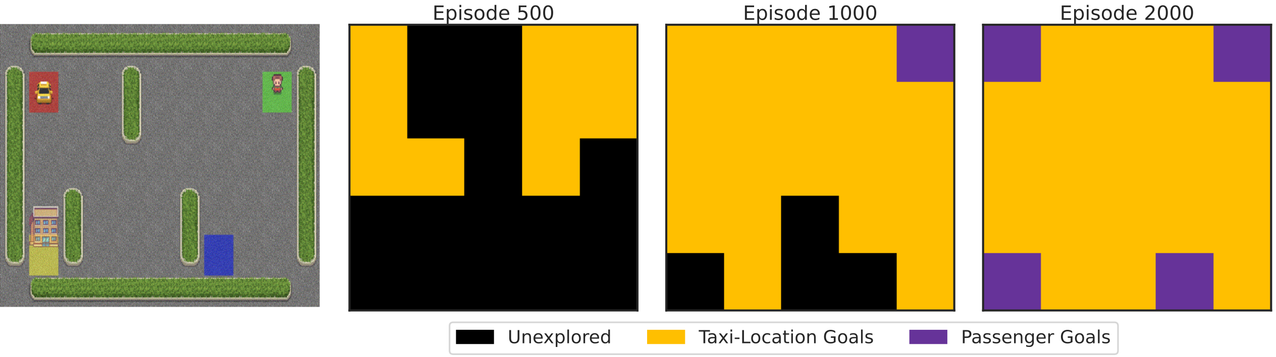
Figure 2: Progression of the goal space refinement in SparseTaxi (domain illustrated in the leftmost sub-figure (Brockman et al., 2016)). This is a visualization of the $5\times 5$ grid; yellow and black squares are explored and unexplored taxi locations respectively; purple squares denote explored passenger locations. The set of plausible goals grows over time from controlling the taxi location, to eventually controlling the location of the passenger. The passenger destination is always deemed uncontrollable by the Proto-goal Evaluator.

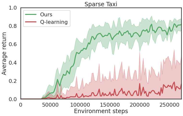
Figure 3: Learning curves comparing Q-learning with $\epsilon$-greedy exploration to proto-goal-based exploration on SparseTaxi. Error bars denote standard error over $20$ independent runs.

5.3 Mastery-based Goal Recombination

We use one simple form of goal recombination in the agent: for any pair of goals that it has mastered, it adds their combination (logical AND) as proto-goal candidate to be evaluated by the PGE. A goal is considered mastered when its success rate is above a pre-specified threshold $\kappa$ ($=0.6$ in all our experiments). For example, if the agent has mastered the goal of getting the key, and another goal of reaching the door, it will combine them to create a new proto-goal which is attained when the agent has reached the door with the key. Implementation details about creating and managing combination proto-goals can be found in the appendix (Algorithm 5).

5.4 Distributed RL Agent Implementation

For all non-toy experiments, we integrate our method with an off-the-shelf distributed RL agent, namely R2D2 (Kapturowski et al., 2018). It is a distributed system of $128$ actors asynchronously interacting with $128$ environments. The learner is Q-learning-based, using a goal-conditioned action-value function $Q_{\theta}(s,a,g)$ parameterized as a UVFA. Experience is stored in a replay buffer $\mathcal{B}$, including the binary proto-goal annotation vector $\mathbf{b}$. More details about the agent, as well as pseudo-code, can be found in Appendix C.

6 Experiments

Our empirical results are designed to establish proto-goal RL an effective way to do exploration, first in a classic tabular set-up (Taxi, Section 6.1), and then at scale in two large-scale domains (NetHack and Baba Is You, Sections 6.3 and 6.4) whose combinatorial proto-goal spaces, left unpruned, would be too large for vanilla goal-conditioned RL. Alongside, ablations and probe experiments show the effectiveness of our controllability and desirability metrics, and provide qualitative insights into the discovered goal spaces.

6.1 Tabular Experiment: Exploration in Taxi

We build intuition about proto-goal exploration on the Taxi domain, a tabular MDP classically used to test hierarchical RL algorithms (Dietterich, 1998). In this problem, the agent controls a taxi in a $5\times 5$ grid; the taxi must first navigate to the passenger, pick them up, take them to their destination (one of $4$) and then drop them off. The default reward function is shaped (Randløv and Alstrøm, 1998), but to make it a harder exploration problem, we propose the SparseTaxi variant, with two changes : (a) no shaping rewards for picking up or dropping off the passenger and (b) the episode terminates when the passenger is dropped off. In other words, the only (sparse) positive reward occurs when the passenger is dropped off at their correct destination.

As proto-goal space, we use a factoring of the state space, namely one $b_{i}$ for each entity (taxi, passenger, destination) in each grid location ($|B|=34$). Figure 2 shows the progression of how the PGE gradually refines a goal space from those throughout training. The set of reachable states expands gradually to mimic a curriculum; at first, goals correspond to navigating the taxi to different locations, later they include goals for dropping off the passenger at different depots. Also noteworthy is that proto-goals corresponding to the destination are absent from the goal space, because they are classified as uncontrollable.

In terms of performance, our proposed method of goal-discovery also leads to more sample-efficient exploration in SparseTaxi (Figure 3). Compared to a vanilla Q-learning agent with $\epsilon$-greedy exploration, our goal-conditioned Q-learning agent learns to reliably and quickly solve the task. More details can be found in Appendix A.

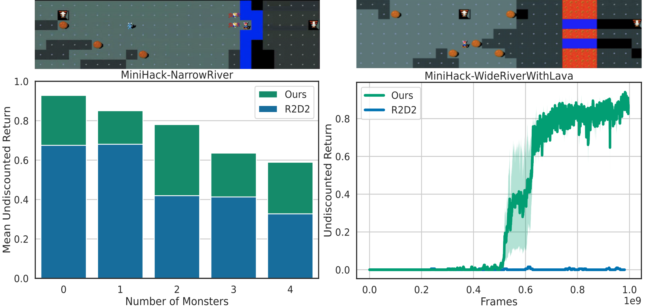
Figure 4: MiniHack experiments. Left: Final performance, when varying difficulty via the number of monsters in NarrowRiver. Right: The challenge of getting off the ground in WideRiverWithLava (no monsters). In all $5+1$ scenarios, using proto-goals outperforms the baseline R2D2 agent. Scenarios are illustrated above the result plots.

6.2 Verifying the Controllability Measure

Our method of measuring controllability using the discrepancy between “seek” and “avoid” values (Section 4.1) is novel, hence we conduct a set of sanity-checks to verify that it can capture controllability in all its guises. Three toy experiments probe three separate types of controllability:

Static controllability:

Proto-goals whose attainment status does not change. The passenger destination in Taxi is a good example of this kind of uncontrollability—while the destination changes between episodes, there is no single transition in the MDP in which it changes.

Time-based controllability:

Some problems have a timer that increments, but is not controllable by the agent. We check whether our controllability metric classifies such time-based proto-goals as plausible, using $4\times 4$ gridworld with a timer that increments from $1$–$100$ (which is the $\max$ number of steps in an episode).

Distractor controllability:

More generally, parts of the observation that change independently of the agent’s actions are distractors for the purpose of controllability. For this test, we use a visual gridworld, where one image channel corresponds to the controllable player, and the two other channels have pixels that light up uniformly at random (Gregor et al., 2016) (often referred to as a “noisy TV” (Schmidhuber, 2010; Burda et al., 2019a)).

For each of these toy setups, we compare our controllability predictions (Eq. 2) to ground-truth labels, and find it to correctly classify which proto-goals are controllable (Figure 6, see Appendix B for details). The prediction quality depends on the amount of data used to estimate the seek/avoid values.

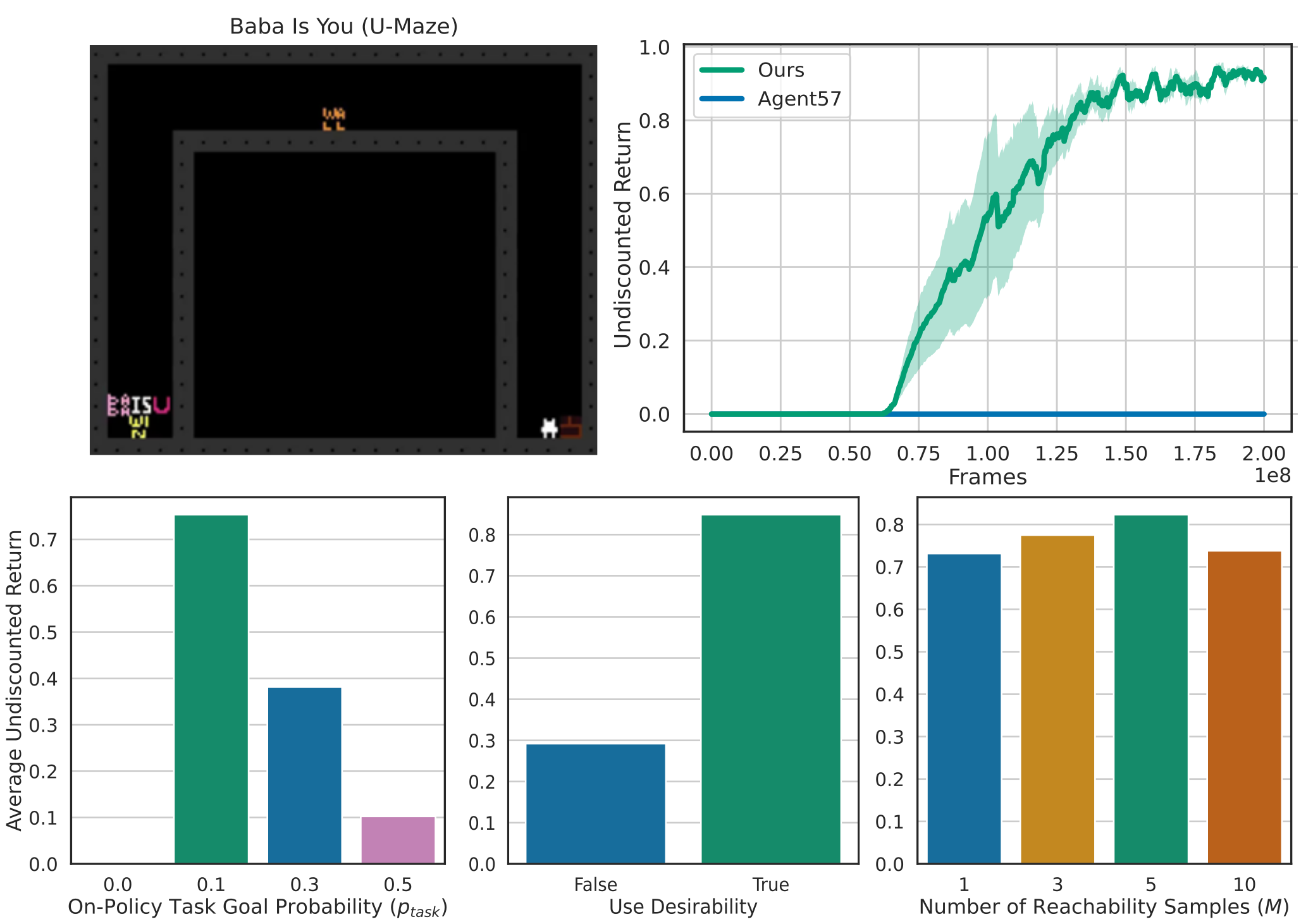
Figure 5: Baba Is You experiments. Top left: U-Maze domain. Top right: Learning curves comparing our approach to (flat-lining) Agent57. Bottom: Ablations showing the importance of sometimes acting according to the task reward during training (left), using desirability metrics in the PGE (middle), and the impact of the number of goals sampled for computing local reachability (right).

6.3 Natural Language Proto-goals: MiniHack

The first large-scale domain we investigate is MiniHack (Samvelyan et al., 2021), a set of puzzles based on the game NetHack (Küttler et al., 2020), which is a grand challenge in RL. In addition to image-based observations, the game also provides natural language messages. This space of language prompts serves as our proto-goal space—while this space is very large (many 1000s of possible sentences), it contains a few useful and interesting goals that denote salient events for the task. Figure 7 illustrates how word-based proto-goal vectors are created in MiniHack.

We use two variants of the River task as exemplary sparse-reward exploration challenges. We choose them because Samvelyan et al. (2021)’s survey noted that while novelty-seeking algorithms (Burda et al., 2019b; Raileanu and Rocktäschel, 2020) could solve the easiest version of River, they were unable to solve more difficult variations.

In all of these, the agent must make a bridge out of boulders and then cross it to reach its goal. In the NarrowRiver variant, the agent needs to place one boulder to create a bridge, and the difficulty depends on the number of monsters who try to kill the player. Figure 4 (left) shows that while increasing the number of monsters degrades performance, our proto-goal agent outperforms the baseline R2D2 agent on each task setting. In the WideLavaRiver variant, the river is wider, requiring $2$ boulders for a bridge, and includes deadly lava that also dissolves boulders. Figure 4 (right) shows that our proto-goal agent comfortably outperforms its baseline.

Discovered goal space.

Words corresponding to important events in the game find their way into the goal-space. For instance, the word “water” appears in the message prompt when the boulder is pushed into the water and when the the player falls into the river and sinks. Later, combination goals like “boulder” AND “water” also appear in the goal-space and require the agent to drop the boulder into the water.

6.4 Doubly Combinatorial Puzzles: Baba Is You

The game Baba Is You (Teikari, 2019) has fascinating emergent complexity. At first sight, the player avatar is a sheep (“Baba”) that can manipulate objects in a 2D space. However, some objects are “word-blocks” that can be arranged into sentences, at which point those sentences become new rules that affect the dynamics of the game (e.g., change the win condition, make walls movable, or let the player control objects other than the sheep with an “X-is-you”-style rule). The natural reward is to reach the (sparse) win condition of the puzzle after $100$s of deliberate interactions.

When testing various RL agents on Baba is You, we observed a common failure mode: the exploration process does not place enough emphasis on manipulating object and text blocks (see also Appendix D.2). So, we created a simple level (U-Maze shown in Figure 5) that is designed to focus on the crucial aspect of rule manipulation. This puzzle requires the agent to learn how to push a word block in place (from center to bottom left), which adds a new win-condition, and then touch the correct block (on the bottom right). Exploration here is challenging because the agent has to master both navigation and block-manipulation before it can get any reward. In addition, the game’s combinatorially large state space is a natural challenge to any novelty-based exploration scheme.

As in Taxi, we use a simple factored proto-goal space, with one binary element for every object (specific word blocks, wall, sheep) being present at any grid-position. Plausible $1$-hot goals could target reaching a specific position of the sheep or movable blocks. Most combinations ($2$-hot proto-goals) are implausible, such as asking the sheep to be in two locations at once, but some could be useful, e.g., targeting particular positions for both “Baba” and a word-block.

Given the exploration challenges in this domain (R2D2 never sees any reward, even on smaller variants of the puzzle), we use the stronger, state-of-the-art Agent57 agent as baseline here, which adds deep exploration on top of R2D2—it constructs an intrinsic reward using novelty and episodic memory (Badia et al., 2020). Figure 5 (top right) shows that our R2D2 with proto-goals (but no intrinsic rewards) outperforms Agent57. Note that with careful tuning, Agent57 does eventually get off the ground on this task, but never within the $200$M frame budget considered here (see Appendix C.1 for details). On the other hand, Agent57 has the advantage that it does not require engineering a proto-goal space.

Discovered goal space.

At first, the goal-space is dominated by navigation goals; once these are mastered, goals that move the word-blocks begin to dominate. Then the agent masters moving to a particular location and moving a word-block to some other location. Eventually, this kind of exploration leads to the agent solving the problem and experiencing the sparse task reward.

Ablations.

Figure 5 (bottom left) analyzes how often the agent should act according to the extrinsic reward instead of picking a goal from the discovered goal-space. When that probability is $0$, the agent never reaches the goal during evaluation; acting according to the task reward function $10\%$ of the time during training performed the best in this setting. In a second ablation, Figure 5 (bottom middle) shows the importance of using desirability metrics on top of plausibility when mapping the proto-goal space to the goal-space. Finally, Figure 5 (bottom right) shows the impact of the number of goals sampled for computing local reachability during goal-selection (Section 5.1). Appendix E details other variants tried, how hyperparameters were tuned, etc.

7 Conclusion and Future Work

We presented a novel approach to using goal-conditioned RL for tackling hard exploration problems. The central contribution is a method that efficiently reduces vast but meaningful proto-goal spaces to a smaller sets of useful goals, using plausibility and desirability criteria based on controllability, reachability, novelty and reward-relevance. Directions for future work include generalising our method to model-based RL to plan with jumpy goal-based models, more fine-grained control on when to switch goals (Pîslar et al., 2022), making the proto-goal space itself learnable, as well as meta-learning the ideal trade-offs between the various desirability criteria.

Appendix A Taxi Details

In Section 6.1, we discussed our experiments with Proto-goal RL on the Taxi domain. Here, we share more details about the problem set up and the agent design.

Proto-goal space.

Each state $s_{t}$ is accompanied by a proto-goal vector $\mathbf{b}_{t}$, which is a $34$ dimensional binary vector: a $25$-bit $1$-hot vector describes the possible taxi locations, a $5$-bit $1$-hot vector describes the passenger location ($4$ depots and $1$ bit to determine whether the passenger is inside the taxi) and a $4$-bit $1$-hot vector describes the passenger’s desired destination. These three $1$-hot vectors are concatenated to form the proto-goal vector $\mathbf{b}_{t}$.

Baseline agent details.

The baseline Q-learning agent maintains a Q-table, $Q:\mathcal{S}\times\mathcal{A}\rightarrow\mathbb{R}$, which is initialized to zero. During training, the agent does $\epsilon$-greedy exploration with $\epsilon=0.1$. Periodically, the agent is tested by rolling out the current greedy policy $\pi=\arg\max_{a}Q(s,a)$ with $\epsilon=0$.

Proto-goal agent details.

Algorithm 1 describes the proto-goal RL agent used for our experiments in tabular taxi. The agent maintains two different Q-tables for each proto-goal $Q_{\text{seek}}^{g}$ and $Q_{\text{avoid}}^{g}$; these Q-tables are first used by the proto-goal evaluator to determine the goal-space $\mathcal{G}$ and subsequently to pick actions conditioned on the goal $g\sim G$ picked for the current episode. All transitions $(s,a,r,s^{\prime})$ are used to update all proto-goal conditioned Q-functions. In addition to learning goal-conditioned Q-functions, the Proto-goal agent maintains one Q-table for the extrinsic reward function $Q(s,a)=\mathbb{E}[R_{1}+R_{2}+\ldots|s_{t}=s,a_{t}=a]$., which is used to greedily pick actions during evaluation.

Algorithm 1 Tabular Proto-goal Agent

1:  Initialize task Q-table: $Q(s,a)=0,\forall{s\in\mathcal{S},a\in\mathcal{A}}.$

2:  Initialize proto-goal Q-tables:

$$Q^{g}_{\text{seek}}(s,a)=Q^{g}_{\text{avoid}}(s,a)=0,\forall{s\in\mathcal{S},a\in\mathcal{A},g\in B}.$$

3:  while training do

4:     Determine goal space: $\mathcal{G}_{t}$=pge($B_{t}$)

5:     Pick a goal $g=$select_goal($s_{t},\mathcal{G}_{t}$)

6:     while not done and not $g$ achieved in $s_{t}$ do

7:        $a_{t}=\arg\max_{a\in\mathcal{A}}Q^{g}_{\text{seek}}(s_{t},a)$

8:        $R_{t},s_{t+1},\mathbf{b}_{t},$ done = env.step($s_{t},a_{t}$)

9:        Add proto-goals $\mathbf{b}_{t}$ to the list of all proto-goals $B_{t}$.

10:        Update the task Q-function using TD-error $\delta_{t}$

$$\delta_{t}=R_{t}+\gamma\max_{a}Q(s_{t+1},a)-Q(s_{t},a_{t}).$$

11:        Update the proto-goal seek Q-functions $\forall g\in B_{t}$

$$\delta^{g}_{t}=r^{g}_{\text{seek}}+\gamma\max_{a}Q_{\text{seek}}^{g}(s_{t+1},a)-Q_{\text{seek}}^{g}(s_{t},a_{t}).$$

12:        Update the proto-goal avoid Q-functions $\forall g\in B_{t}$

$$\delta^{g}_{t}=r_{\text{avoid}}^{g}+\gamma\max_{a}Q_{\text{avoid}}^{g}(s_{t+1},a)-Q_{\text{avoid}}^{g}(s_{t},a_{t}).$$

13:     end while

14:  end while

Algorithm 2 Actor::select_goal()

Inputs: Goal space $\mathcal{G}$, current state $s_{t}$
Output: Goal to pursue at $s_{t}$
Hyperparameters: Number of timescale bins $k$, number of novel goals $m$, task reward probability $p_{task}$.

1:  if random.random()$<p_{task}$ then

2:     return $g_{t}=\mathbf{0}$

3:  else

4:     Bin goals $\mathcal{G}=\{\mathcal{G}_{1},...,\mathcal{G}_{k}\}$ based on timescale.

5:     Uniformly sample a bin from $\mathcal{G}$: $\mathcal{G}^{h}=\{g_{1},...,g_{n}\}$.

6:     Sample (with replacement) a set $G=\{g_{1},...,g_{m}\}$ from $\mathcal{G}^{h}$ based on novelty.

7:     Pick nearest goal in $G$: $g_{t}=\arg\max_{g\in G}\Big{[}V_{\theta}(s_{t}|g)\Big{]}$

8:     return $g_{t}$

9:  end if

Algorithm 3 PGE::get_plausible_proto_goals()

Inputs: Proto-goals observed so far $B_{t}$, replay buffer $\mathcal{B}$.
Hyperparameters: Controllability threshold $\tau_{1}$, reachability threshold $\tau_{2}$.

1:  Sample transitions from replay: $s,a,s^{\prime}\sim\mathcal{B}$.

2:  Relabel transitions based on seek reward function: $r^{g}_{\text{seek}}=R_{\text{seek}}(s,s^{\prime},g)$, $\forall{g}\in B_{t}$.

3:  Relabel transitions based on avoid reward function: $r^{g}_{\text{avoid}}=R_{\text{avoid}}(s,s^{\prime},g)$, $\forall{g}\in B_{t}$.

4:  Train seek value-function for each proto-goal: $V_{\text{seek}}^{g}=$LSPI($s,a,r^{g}_{\text{seek}},s^{\prime}$), $\forall{g}\in B_{t}$.

5:  Train avoid value-function for each proto-goal: $V_{\text{avoid}}^{g}=$LSPI($s,a,r^{g}_{\text{avoid}},s^{\prime}$), $\forall{g}\in B_{t}$.

6:  Get the controllable proto-goals:

$$\mathcal{C}=\Big{\{}g:\mathbb{E}_{s}\Big{[}V_{\text{seek}}^{g}(s)+V_{\text{avoid}}^{g}(s)\Big{]}<\tau_{1},\forall{g}\in B_{t}\Big{\}}.$$

7:  Plausible ones are the sometimes-reachable subset:

$$\mathcal{G}=\Big{\{}g:\max_{s}V^{g}_{\text{seek}}(s)>\tau_{2},\forall{g}\in\mathcal{C}\Big{\}}.$$

8:  return plausible proto-goals $\mathcal{G}$.

Algorithm 4 PGE::get_desirable_goals()

Inputs: Plausible proto-goals $\mathcal{G}$, mapping of proto-goals to counts $N:\mathcal{G}\rightarrow\mathbb{N}$, mapping of proto-goals to average reward $R:\mathcal{G}\rightarrow\mathbb{R}$.
Hyperparameters: Size of goal set $K$.

1:  Assign each proto-goal a desirability score:

$$u(g)=R(g)+\frac{1}{\sqrt{N(g)}},\forall{g\in\mathcal{G}}.$$

2:  Convert the desirability score to probabilities:

$$\mathbb{P}(g)=\frac{u(g)}{\sum_{g}u(g)},\forall{g\in\mathcal{G}}.$$

3:  Sample with replacement $G$, a set of $K$ goals from plausible proto-goals $\mathcal{G}$ using desirability probabilities $\mathbb{P}(g)$.

4:  return goal set $G$.

Algorithm 5 PGE::get_combination_proto_goals()

Inputs: Goal space $\mathcal{G}$, mapping of goals to counts $N:\mathcal{G}\rightarrow\mathbb{N}$, mapping of goals to the average success ratio on the last $10$ on-policy pursuits $S:\mathcal{G}\rightarrow[0,1]$.
Hyperparameters: Mastery threshold $\kappa$.

1:  Mastered goals $M$:

$$M=\{g|g\in\mathcal{G},N(g)\geq 10,S(g)>\kappa\}$$

2:  Convert the mastery scores to probabilities:

$$\mathbb{P}(g)=\frac{S(g)}{\sum_{g}S(g)},\forall{g\in M}.$$

3:  Sample (without replacement) $2$ goals from $\mathbb{P}(g):g_{1},g_{2}$.

4:  Create new proto-goal $\mathbf{b}=$ AND($g_{1},g_{2}$) and add it to the proto-goal space $B_{t}$.

5:  return $B_{t}$

Algorithm 6 Actor::run_loop()

Inputs: Proto-goal evaluator pge.
Hyperparameters: Number of goals to replay $M_{her}$.

1:  while true do

2:     $g=$select_goal($s_{t}$).

3:     Sample trajectory $\tau_{g}=\{s,a,r_{g},s^{\prime},b\}$ by rolling out goal-conditioned policy $\pi_{\theta}(s_{t}|g).$

4:     Add $\tau_{g}$ to the replay buffer.

5:     Get $\mathcal{G}_{A}$, the set of goals achieved during $\tau_{g}$.

6:     Sample $\mathcal{G}_{A}^{\text{novel}}$ without replacement from $\mathcal{G}_{A}$, a set of $\min(M_{her},|\mathcal{G}_{A}|)$ goals, proportionally to $\frac{1}{\sqrt{N(g)}}$.

7:     Relabel trajectory $\tau_{g}$, once for each goal in $\mathcal{G}_{A}^{\text{novel}}$.

8:     Relabel trajectory $\tau_{g}$ with extrinsic reward.

9:     Add relabeled trajectories to the replay buffer.

10:     Use $\tau_{g}$ to update the proto-goal buffer $B_{t}$, their counts and their average reward.

11:  end while

Appendix B Details of Controllability Experiments

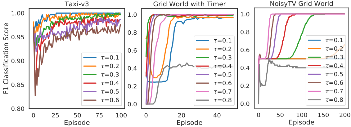
Figure 6: Testing our seek-avoid controllability measure in toy domains using the F1 classification metric. In each domain, we collect transitions using a random policy and measure how effectively we can classify controllability for different values of the threshold $\tau_{1}$.

In each of the toy problem setups described in Section 6.2 of the main paper, we roll out a random policy and store the collected transitions in memory. At the end of each episode, we re-train the seek- and avoid-value functions on all transitions, as discussed in Section 4.1.1, and use Eq. 2 to classify whether or not different proto-goals are controllable. We then test the predicted classification labels against the ground-truth labels using the F1-classification score.

Results.

Figure 6 shows we are able to correctly classify proto-goals as controllable vs uncontrollable in each of the aforementioned cases. These results also suggest that training the seek-avoid value functions using more data improves classification performance.

Appendix C Details of the Proto-R2D2 Agent

Figure 7: Proto-goal space in MiniHack: the message part of the observation is converted to a binary vector $b_{t}$ using bag-of-words.

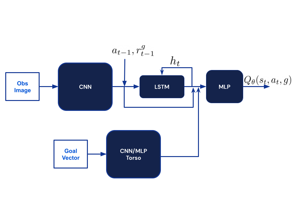
Figure 8: UVFA Architecture used to learn $Q_{\theta}(s,a,g)$.

Figure 9: System architecture of the Proto-goal R2D2 Agent. Gray blocks denote components shared with baseline R2D2, blue blocks denote components added for Proto-goal RL.

We now describe the details of the agent used to produce the results in Sections 6.3 and 6.4. The R2D2 algorithm (Kapturowski et al., 2018) forms the basis for the Proto-R2D2 agent; so, there are $128$ actors interacting with $128$ copies of the environment.

These actors follow the process described in Algorithm 6. The goal-conditioned value-function (UVFA) used to select actions in line 3 is parameterized using the network architecture shown in Figure 8. This UVFA is trained using R2D2’s version of Q-learning on batches randomly sampled from the replay buffer $\{s,a,r_{g},s^{\prime},g\}\sim\mathcal{B}$. As shown in Figure 9, each of the actors stream the proto-goals that they observe to the proto-goal evaluator (PGE), which maintains the buffer $B_{t}$ of ever-seen proto-goals, with the number of times each proto-goal has been achieved $N(g)$. Each actor also streams the extrinsic reward observed when each proto-goal was achieved; this information is also streamed to the PGE, which keeps a running mean of the rewards.

The PGE asynchronously samples from replay and determines the goal-space for goal-conditioned RL. It first prunes the proto-goal buffer $B_{t}$ using plausibility metrics as described in Algorithm 3. Then, it samples a smaller space of goals using desirability metrics as described in Algorithm 4. This goal-space is subsequently used in the next actor/learner iteration.

The evaluator is another process that asynchronously interacts with its own copy of the environment; the rewards it experiences are reported in the learning curves in Figures 4 and 5 (main paper). The evaluator also picks actions using the UVFA parameters $\theta$, but it always conditions the UVFA on task reward-function (using $g=\mathbf{0}$ as discussed in the main paper). Following Badia et al. (2020), all our learning curves are averaged over $3$ random seeds.

C.1 Agent57 Baseline

We performed a grid search over Agent57 hyperparameters episodic_memory_reward_scale$=\{0,0.01,0.001\}$ and meta_episode_length$=\{1,5,10\}$ on the U-Maze task. meta_episode_length represents the number of episodes after which the episodic memory is reset, episodic_memory_reward_scale modulates the contribution of the episodic memory to the intrinsic reward (Badia et al., 2020). Out of these, episodic_memory_reward_scale of $0.001$ and meta_episode_length of $10$ performed the best; the results presented in the paper use these hyperparameters. None of these configurations get off the ground in the $200$ million frames range considered here; however, we have evidence that, when trained up to $1$ billion frames, Agent57 with the chosen hyperparameters can solve U-Maze.

Appendix D More Details about Test Environments

In this section, we outline some more details about the set up for our MiniHack and Baba Is You experiments.

D.1 MiniHack

The puzzle is procedurally generated every episode. The action space in our tasks was all $8$ compass directions. The tasks are partially observable—not all tiles are visible to the agent at all times; the player must go close to a tile to reveal its contents. Even when the number of monsters is configured to $0$, because of the dynamics of NetHack, there is always some probability that a monster will spawn in a tile. Episodes last for a maximum of $350$ steps, unless the player reaches the goal, in which case the episode terminates with a sparse reward of $1$.

D.2 Baba Is You

We use a DMLab (Beattie et al., 2016) implementation of the popular game Baba Is You (Teikari, 2019). The observation is a stack of 2D images: each image in the stack corresponds to a single object. For example, one image plane represents the sheep baba, while another image plane represents the word-block “baba”. Since there are $7$ objects in the U-Maze level, each observation is a $2$D image with $7$ channels. There are $5$ actions in the action-space: up, down, left, right and no-op. Episodes last for a maximum of $1000$ steps. If there is no rule that specifies that X-IS-YOU (where X is any object), then the episode terminates with a reward of $0$ (because there is nothing left to control); if the agent reaches whatever object forms the win condition (as in Y-IS-WIN), then the episode terminates with a sparse reward of $1$.

The preliminary experiments that let to the design to the U-Maze used various RL agents, including V-trace-based planning agents, R2D2, Q-learning, Agent57, tested on different (early) in-game levels of Baba is You.

Appendix E Further Ablations and Variants Tried

In this section, we discuss some of the strategies that did not work and some strategies we used to set the values of certain hyperparameters.

1. Importance of the timescale-based stratification: without timescale stratification (Section 5.1), the local reachability metric always hurt performance, likely because it biased goal-selection towards easy goals. After incorporating stratified sampling, using local reachability outperformed only using novelty for goal-selection and allowed the agent to condition the higher-level policy on the current state.

2. Number of hindsight goals replayed: Each trajectory is used to replay a maximum of $M_{her}=15$ achieved goals in hindsight (Section 5.2). We swept over this value: performance tends to follow the familiar U-shaped curve—replaying too few or too many goals degrades performance.

3. Importance of the plausibility metrics: without the use of the plausibility heuristics discussed in Section 4.1, the system drowns in goals it can never achieve. For example, the vast majority of combination goals are implausible and yet they are very novel; without pruning, these goals dominate the goal-space and prevent true competence progress.

Parameter	Value
Replay buffer size	$1e6$
Prioritized experience replay∗	False
Optimizer	Adam
Learning rate	$3\cdot 10^{-4}$
Adam hyper-parameters	$\beta_{1}=0.9$
	$\beta_{2}=0.999$
	$\epsilon=10^{-4}$
Weight decay	$10^{-4}$
Target net update period	$1e4$
Batch size	64
Discount factor $\gamma$	0.99
Trace length∗	10
Trace $\lambda$	0.95

Table 1: Inherited R2D2 Hyperparameters. These are essentially untuned except for those marked with ^∗ (see Section F).

Parameter	Value	Tuned?
Sampled goal set size $K$	$100$	no
Number of goals to replay $M_{her}$	$15$	yes
Controllability threshold $\tau_{1}$	$0.1$	yes
Reachability threshold $\tau_{2}$	$0.5$	no
Number of random projections $|\phi|$	32	no
LSPI batch size	$1024$	no
LSPI discount factor	$0.95$	no
Task reward probability $p_{task}$	$0.1$	yes
Number of timescale buckets $k$	$5$	no
Number of novelty goals to sample $M$	$5$	no
Mastery threshold $\kappa$	$0.6$	yes
Number of seeds	3	N/A

Table 2: Specific Proto-R2D2 hyperparameters.

Appendix F Hyperparameters

Table 1 lists the parameter settings for the R2D2 agent; Table 2 shows the settings for the hyperparameters specifically added by our algorithm. Here is the rationale for picking the values of some of the hyperparameters:

1. LSPI batch size: this is the batch size for computing the seek/avoid value-functions. We used $1024$ because that was the largest batch size for which the wall-clock time for training was still reasonable.

2. Number of random projections: we followed Ghavamzadeh et al. (2010) and set this to the square-root of the number of transitions in the minibatch. Since this heuristic worked well, we did not tune the number of random projections any further.

3. Controllability threshold: we used $0.1$ because it worked well in smaller domains in which we could measure the F1 classification score against the ground-truth controllable goals (see Figure 6).

4. Number of timescale buckets: we manually looked at goal-spaces with different values of $k$. When $k=5$, the goal-space divided into goal buckets that intuitively segmented based on increasing difficulty.

5. Trace length: R2D2 typically uses a larger trace length (Kapturowski et al., 2018). Unlike Atari games, our tasks can have much shorter episode lengths (due to goal terminations), so we used a shorter trace length.

6. Prioritization: we did not use prioritized experience replay (PER) (Schaul et al., 2016) because it would significantly increase computation and implementation complexity. More specifically, to replay a trajectory with an off-policy goal, we would have to recompute TD errors with respect the hindsight goal’s reward function. Due to the added computation and implementation complexity (and because this was not our core contribution), we did not use prioritization.

Network architecture.

Figure 8 shows the network architecture for the goal-conditioned Q-function. The network architecture is identical to R2D2 (Kapturowski et al., 2018) except for the fact that the goal is processed by its own CNN (when it is an image as in Baba Is You) or by an MLP (when the goal is a flattened binary vector as in MiniHack); the architecture of the goal-processing CNN/MLP is identical to the corresponding blocks in R2D2.

Hyperparameter sensitivity.

In general, we found that the proto-goal agent was robust to different settings of the majority of hyperparamters in Table 2, with the exception of the task goal probability $p_{task}$, whose different settings resulted in qualitatively different performances (see Figure 5).

References

- Abel [2020] David Abel. A Theory of Abstraction in Reinforcement Learning. PhD thesis, Brown University, 2020.
- Andrychowicz et al. [2017] Marcin Andrychowicz, Dwight Crow, Alex Ray, Jonas Schneider, Rachel Fong, Peter Welinder, Bob McGrew, Josh Tobin, Pieter Abbeel, and Wojciech Zaremba. Hindsight experience replay. In Advances in Neural Information Processing Systems 30, 2017, pages 5048–5058, 2017.
- Auer [2002] Peter Auer. Using confidence bounds for exploitation-exploration trade-offs. Journal of Machine Learning Research, 3(Nov):397–422, 2002.
- Bacon et al. [2017] Pierre-Luc Bacon, Jean Harb, and Doina Precup. The option-critic architecture. In Proceedings of the AAAI Conference on Artificial Intelligence, volume 31, 2017.
- Badia et al. [2020] Adrià P. Badia, Bilal Piot, Steven Kapturowski, Pablo Sprechmann, Alex Vitvitskyi, Zhaohan Daniel Guo, and Charles Blundell. Agent57: Outperforming the Atari human benchmark. In International Conference on Machine Learning, pages 507–517, 2020.
- Bagaria and Konidaris [2020] Akhil Bagaria and George Konidaris. Option discovery using deep skill chaining. In International Conference on Learning Representations, 2020.
- Bagaria et al. [2021] Akhil Bagaria, Jason K. Senthil, and George Konidaris. Skill discovery for exploration and planning using deep skill graphs. In International Conference on Machine Learning, pages 521–531. PMLR, 2021.
- Barreto et al. [2019] André Barreto, Diana Borsa, Shaobo Hou, Gheorghe Comanici, Eser Aygün, Philippe Hamel, Daniel Toyama, Shibl Mourad, David Silver, and Doina Precup. The option keyboard: Combining skills in reinforcement learning. Advances in Neural Information Processing Systems, 32, 2019.
- Beattie et al. [2016] Charles Beattie, Joel Z Leibo, Denis Teplyashin, Tom Ward, Marcus Wainwright, Heinrich Küttler, Andrew Lefrancq, Simon Green, Víctor Valdés, Amir Sadik, et al. Deepmind lab. arXiv preprint arXiv:1612.03801, 2016.
- Bellemare et al. [2016] Marc Bellemare, Sriram Srinivasan, Georg Ostrovski, Tom Schaul, David Saxton, and Remi Munos. Unifying count-based exploration and intrinsic motivation. Advances in neural information processing systems, 29, 2016.
- Brockman et al. [2016] Greg Brockman, Vicki Cheung, Ludwig Pettersson, Jonas Schneider, John Schulman, Jie Tang, and Wojciech Zaremba. Openai gym. arXiv preprint arXiv:1606.01540, 2016.
- Burda et al. [2019a] Yuri Burda, Harrison Edwards, Deepak Pathak, Amos J. Storkey, Trevor Darrell, and Alexei A. Efros. Large-scale study of curiosity-driven learning. In International Conference on Learning Representations, ICLR, 2019.
- Burda et al. [2019b] Yuri Burda, Harrison Edwards, Amos Storkey, and Oleg Klimov. Exploration by random network distillation. In International Conference on Learning Representations, 2019.
- Campos et al. [2020] Víctor Campos, Alexander Trott, Caiming Xiong, Richard Socher, Xavier Giró-i Nieto, and Jordi Torres. Explore, discover and learn: Unsupervised discovery of state-covering skills. In International Conference on Machine Learning, 2020.
- Chentanez et al. [2004] Nuttapong Chentanez, Andrew Barto, and Satinder Singh. Intrinsically motivated reinforcement learning. Advances in neural information processing systems, 17, 2004.
- Dietterich [1998] Thomas Dietterich. The MAXQ method for hierarchical reinforcement learning. In ICML, volume 98, pages 118–126, 1998.
- Eysenbach et al. [2018] Benjamin Eysenbach, Abhishek Gupta, Julian Ibarz, and Sergey Levine. Diversity is all you need: Learning skills without a reward function. In International Conference on Learning Representations, 2018.
- Forestier et al. [2022] Sébastien Forestier, Rémy Portelas, Yoan Mollard, and Pierre-Yves Oudeyer. Intrinsically motivated goal exploration processes with automatic curriculum learning. Journal of Machine Learning Research (JMLR), 2022.
- Fortunato et al. [2018] Meire Fortunato, Mohammad G. Azar, Bilal Piot, Jacob Menick, Ian Osband, Alex Graves, Vlad Mnih, Remi Munos, Demis Hassabis, Olivier Pietquin, Charles Blundell, and Shane Legg. Noisy networks for exploration. International Conference on Learning Representations, ICLR, 2018.
- Gershman [2017] Samuel J. Gershman. On the blessing of abstraction. Quarterly Journal of Experimental Psychology, 70:361 – 365, 2017.
- Ghavamzadeh et al. [2010] Mohammad Ghavamzadeh, Alessandro Lazaric, Odalric Maillard, and Rémi Munos. LSTD with random projections. Advances in Neural Information Processing Systems, 23, 2010.
- Gregor et al. [2016] Karol Gregor, Danilo J. Rezende, and Daan Wierstra. Variational intrinsic control. arXiv preprint arXiv:1611.07507, 2016.
- Jaderberg et al. [2017] Max Jaderberg, Volodymyr Mnih, Wojciech Marian Czarnecki, Tom Schaul, Joel Z Leibo, David Silver, and Koray Kavukcuoglu. Reinforcement learning with unsupervised auxiliary tasks. 5th International Conference on Learning Representations, ICLR, 2017.
- Kaplan and Oudeyer [2004] Frédéric Kaplan and Pierre-Yves Oudeyer. Maximizing learning progress: an internal reward system for development. In Embodied artificial intelligence, pages 259–270. Springer, 2004.
- Kapturowski et al. [2018] Steven Kapturowski, Georg Ostrovski, John Quan, Remi Munos, and Will Dabney. Recurrent experience replay in distributed reinforcement learning. In International conference on learning representations, 2018.
- Konidaris and Barto [2009] George Konidaris and Andrew Barto. Skill discovery in continuous reinforcement learning domains using skill chaining. Advances in neural information processing systems, 22, 2009.
- Konidaris [2019] George Konidaris. On the necessity of abstraction. Current opinion in behavioral sciences, 29:1–7, 2019.
- Küttler et al. [2020] Heinrich Küttler, Nantas Nardelli, Alexander Miller, Roberta Raileanu, Marco Selvatici, Edward Grefenstette, and Tim Rocktäschel. The NetHack learning environment. Advances in Neural Information Processing Systems, 33:7671–7684, 2020.
- Lagoudakis and Parr [2003] Michail G. Lagoudakis and Ronald Parr. Least-squares policy iteration. The Journal of Machine Learning Research, 2003.
- Lillicrap et al. [2016] Timothy P. Lillicrap, Jonathan J. Hunt, Alexander Pritzel, Nicolas Heess, Tom Erez, Yuval Tassa, David Silver, and Daan Wierstra. Continuous control with deep reinforcement learning. In International Conference on Learning Representations, ICLR, 2016.
- Lin [1993] Long-Ji Lin. Reinforcement learning for robots using neural networks. Technical report, Carnegie-Mellon Univ Pittsburgh PA School of Computer Science, 1993.
- Liu et al. [2022] Minghuan Liu, Menghui Zhu, and Weinan Zhang. Goal-conditioned reinforcement learning: Problems and solutions. arXiv preprint arXiv:2201.08299, 2022.
- Lopes et al. [2012] Manuel Lopes, Tobias Lang, Marc Toussaint, and Pierre-Yves Oudeyer. Exploration in model-based reinforcement learning by empirically estimating learning progress. Advances in neural information processing systems, 25, 2012.
- Machado et al. [2017] Marlos C. Machado, Marc G. Bellemare, and Michael Bowling. A Laplacian framework for option discovery in reinforcement learning. In International Conference on Machine Learning, pages 2295–2304. PMLR, 2017.
- Mohamed and Rezende [2015] Shakir Mohamed and Danilo Rezende. Variational information maximisation for intrinsically motivated reinforcement learning. Advances in neural information processing systems, 28, 2015.
- Osband et al. [2016] Ian Osband, Charles Blundell, Alexander Pritzel, and Benjamin Van Roy. Deep exploration via bootstrapped DQN. Advances in neural information processing systems, 29, 2016.
- Osband et al. [2018] Ian Osband, John Aslanides, and Albin Cassirer. Randomized prior functions for deep reinforcement learning. Advances in Neural Information Processing Systems, 31, 2018.
- Ostrovski et al. [2021] Georg Ostrovski, Pablo Samuel Castro, and Will Dabney. The difficulty of passive learning in deep reinforcement learning. In Advances in Neural Information Processing Systems, volume 34, pages 23283–23295, 2021.
- Pathak et al. [2017] Deepak Pathak, Pulkit Agrawal, Alexei A. Efros, and Trevor Darrell. Curiosity-driven exploration by self-supervised prediction. In International conference on machine learning, 2017.
- Pîslar et al. [2022] Miruna Pîslar, David Szepesvari, Georg Ostrovski, Diana Borsa, and Tom Schaul. When should agents explore? In International Conference on Learning Representations (ICLR), 2022.
- Pitis et al. [2020] Silviu Pitis, Harris Chan, Stephen Zhao, Bradly Stadie, and Jimmy Ba. Maximum entropy gain exploration for long horizon multi-goal reinforcement learning. In Proceedings of the 37th International Conference on Machine Learning, ICML 2020, volume 119, pages 7750–7761, 2020.
- Plappert et al. [2018] Matthias Plappert, Rein Houthooft, Prafulla Dhariwal, Szymon Sidor, Richard Y. Chen, Xi Chen, Tamim Asfour, Pieter Abbeel, and Marcin Andrychowicz. Parameter space noise for exploration. International Conference on Learning Representations, ICLR, 2018.
- Pong et al. [2019] Vitchyr H. Pong, Murtaza Dalal, Steven Lin, Ashvin Nair, Shikhar Bahl, and Sergey Levine. Skew-fit: State-covering self-supervised reinforcement learning. Proceedings of the 37th International Conference on Machine Learning, ICML, 2019.
- Raileanu and Rocktäschel [2020] Roberta Raileanu and Tim Rocktäschel. RIDE: Rewarding impact-driven exploration for procedurally-generated environments. In International Conference on Learning Representations, 2020.
- Randløv and Alstrøm [1998] Jette Randløv and Preben Alstrøm. Learning to drive a bicycle using reinforcement learning and shaping. In ICML, volume 98, pages 463–471. Citeseer, 1998.
- Ring [1994] Mark B. Ring. Continual learning in reinforcement environments. PhD thesis, University of Texas at Austin, Texas, 1994.
- Samvelyan et al. [2021] Mikayel Samvelyan, Robert Kirk, Vitaly Kurin, Jack Parker-Holder, Minqi Jiang, Eric Hambro, Fabio Petroni, Heinrich Küttler, Edward Grefenstette, and Tim Rocktäschel. MiniHack the planet: A sandbox for open-ended reinforcement learning research. In NeurIPS Datasets and Benchmarks Track, 2021.
- Schaul and Ring [2013] Tom Schaul and Mark B. Ring. Better generalization with forecasts. In IJCAI, pages 1656–1662, 2013.
- Schaul et al. [2015] Tom Schaul, Daniel Horgan, Karol Gregor, and David Silver. Universal value function approximators. In Proceedings of the 32nd International Conference on Machine Learning, ICML, volume 37, pages 1312–1320, 2015.
- Schaul et al. [2016] Tom Schaul, John Quan, Ioannis Antonoglou, and David Silver. Prioritized experience replay. 4th International Conference on Learning Representations, ICLR, 2016.
- Schaul et al. [2019] Tom Schaul, Diana Borsa, Joseph Modayil, and Razvan Pascanu. Ray interference: a source of plateaus in deep reinforcement learning. arXiv preprint arXiv:1904.11455, 2019.
- Schmidhuber [1991] Jürgen Schmidhuber. Curious model-building control systems. In Proc. international joint conference on neural networks, pages 1458–1463, 1991.
- Schmidhuber [2010] Jürgen Schmidhuber. Formal theory of creativity, fun, and intrinsic motivation (1990–2010). IEEE transactions on autonomous mental development, 2(3):230–247, 2010.
- Strehl and Littman [2008] Alexander L. Strehl and Michael L. Littman. An analysis of model-based interval estimation for Markov decision processes. Journal of Computer and System Sciences, 74(8):1309–1331, 2008.
- Sutton and Barto [2018] Richard S. Sutton and Andrew G. Barto. Reinforcement learning: An introduction. MIT press, 2018.
- Sutton et al. [1999] Richard S. Sutton, Doina Precup, and Satinder Singh. Between MDPs and semi-MDPs: A framework for temporal abstraction in reinforcement learning. Artificial Intelligence, pages 181–211, 1999.
- Sutton et al. [2011] Richard S. Sutton, Joseph Modayil, Michael Delp, Thomas Degris, Patrick M. Pilarski, Adam White, and Doina Precup. Horde: A scalable real-time architecture for learning knowledge from unsupervised sensorimotor interaction. In The 10th International Conference on Autonomous Agents and Multiagent Systems-Volume 2, pages 761–768, 2011.
- Sutton et al. [2022] Richard S. Sutton, Michael H. Bowling, and Patrick M. Pilarski. The Alberta plan for AI research. arXiv preprint arXiv:2208.11173, 2022.
- Sutton [1988] Richard S. Sutton. Learning to predict by the methods of temporal differences. Machine learning, 3(1):9–44, 1988.
- Taiga et al. [2020] Adrien Ali Taiga, William Fedus, Marlos C. Machado, Aaron Courville, and Marc G. Bellemare. On bonus based exploration methods in the arcade learning environment. In International Conference on Learning Representations, 2020.
- Tasse et al. [2022] Geraud N. Tasse, Benjamin Rosman, and Steven James. World value functions: Knowledge representation for learning and planning. arXiv preprint arXiv:2206.11940, 2022.
- Teikari [2019] Arvi Teikari. Baba is you. Game [PC], Hempuli Oy, Finland, 2019.
- Veeriah et al. [2019] Vivek Veeriah, Matteo Hessel, Zhongwen Xu, Janarthanan Rajendran, Richard L. Lewis, Junhyuk Oh, Hado van Hasselt, David Silver, and Satinder Singh. Discovery of useful questions as auxiliary tasks. Advances in Neural Information Processing Systems, 32, 2019.
- Veeriah et al. [2021] Vivek Veeriah, Tom Zahavy, Matteo Hessel, Zhongwen Xu, Junhyuk Oh, Iurii Kemaev, Hado van Hasselt, David Silver, and Satinder Singh. Discovery of options via meta-learned subgoals. Advances in Neural Information Processing Systems, 34:29861–29873, 2021.