On some analytic properties of nabla tempered fractional calculus

Abstract

Despite many applications regarding fractional calculus have been reported in literature, it is still unknown how to model some practical process. One major challenge in solving such a problem is that, the nonlocal property is needed while the infinite memory is undesired. Under this context, a new kind nabla fractional calculus accompanied by a tempered function is formulated. However, many properties of such fractional calculus needed to be discovered. From this, this paper gives particular emphasis to the topic. Some remarkable properties like the equivalence relation, the nabla Taylor formula, and the nabla Laplace transform for such nabla fractional calculus are developed and analyzed. It is believed that this work greatly enriches the mathematical theory of nabla tempered fractional calculus and provides high value and huge potential for further applications.

1 Introduction

Fractional calculus, as a powerful toolbox, has attracted an increasing attention from scholars in the past decades [1, 2, 3, 4]. Due to its nonlocal property, fractional calculus play a key role in diverse application of science and engineering. Also, nonlocal property brings many difficulties and challenges in modeling some special objects. From this, the past decade has witnessed a significant progress on tempered fractional calculus by introducing an extra weighted function. Notably, tempered fractional calculus has many merits, and henceforth many researchers have deployed themselves to explore valuables results. A huge work has been done for this subject [5, 6, 7, 8], which makes a positive and profound impact.

Compared with the continuous time case, the research in discrete time case is just in its infancy and only few work has been reported preliminarily. I have to admit that the discrete time case performs better in computing, storage, transport than the continuous time case and it has greater potential in the digital era. The memory effect of delta tempered fractional calculus was investigated and applied to image processing [9]. The tempered fractional derivative on an isolated time scale was defined and a new method was presented based on the time scale theory for numerical discretization in [10]. A general definition for nabla discrete time tempered fractional calculus was presented in [11]. The tempered function was chosen as the nonzero case instead of the discrete exponential function, which greatly enrich the potential of the tempered fractional calculus. Though the study on discrete time tempered fractional calculus is still in sufficient, a proliferation of results reported on discrete time fractional calculus [12, 13, 14, 15] could give us a lot of helpful inspiration.

The basic arithmetic and equivalence relations of fractional difference and fractional sum were discussed in [12, 13, 14, 16]. The continuity on the order of fractional difference was studied in [12, 14, 17]. However, the Grünwald–Letnikov difference is not equivalent to the classical integer order case for integral order, which means that the existing results need extra conditions. The nabla Taylor series was first investigated systematically in [17], while some of the existing results requires quite strict conditions and the nabla Taylor formula expanded at the current time was not discussed enough. A brief review was made on the nabla Laplace transform [18] and some interesting properties still could be built with the existing results. It is worth noting that some similar properties like the classical case can be checked for the tempered case and some seminal properties for the tempered case need to be investigated. Bearing this in mind, some fundamental properties will be developed carefully. However, it is not an easy task to complete this task, since the introduction of the tempered function brings some unexpected difficulty and damage some accustomed properties.

The main contribution of this work lies in the following aspects. (i) The relationship between nabla tempered fractional difference/sum is explored. (ii) The nabla Taylor formula/series representation of nabla tempered fractional calculus is developed. (iii) The nabla Laplace transform for nabla tempered fractional difference/sum is derived. Hopefully, these distinguished properties could be helpful for other researchers understand and apply such fractional calculus.

The remainder of this paper is summarized as follows. In Section 2, the basic concept and properties of nabla tempered fractional calculus are presented here. In Section 3, many foundational properties are developed for such fractional calculus. In Section 4, some concluding remarks are provided to end this paper.

2 Preliminaries

In this section, the definitions and properties for nabla tempered fractional calculus are introduced.

For $x:\mathbb{N}_{a+1-n}\to\mathbb{R}$, its $n$-th nabla difference is defined by

$${\textstyle\nabla^{n}x(k):=\sum_{i=0}^{n}(-1)^{i}\big{(}\begin{smallmatrix}n\\ i\end{smallmatrix}\big{)}x(k-i),}$$ (1)

where $n\in\mathbb{Z}_{+}$, $k\in\mathbb{N}_{a+1}:=\{a+1,a+2,\cdots\}$, $a\in\mathbb{R}$, $\left(\begin{smallmatrix}p\\ q\end{smallmatrix}\right):=\frac{\Gamma(p+1)}{\Gamma(q+1)\Gamma(p-q+1)}$ is the generalized binomial coefficient and $\Gamma(\cdot)$ is the Gamma function.

For $x:\mathbb{N}_{a+1}\to\mathbb{R}$, its $\alpha$-th Grünwald–Letnikov difference/sum is defined by [13, 19]

$${\textstyle{}_{a}^{\rm G}\nabla_{k}^{\alpha}x(k):=\sum_{i=0}^{k-a-1}(-1)^{i}\big{(}\begin{smallmatrix}\alpha\\ i\end{smallmatrix}\big{)}x(k-i),}$$ (2)

where $\alpha\in\mathbb{R}$, $k\in\mathbb{N}_{a+1}$ and $a\in\mathbb{R}$. When $\alpha>0$, ${}_{a}^{\rm G}\nabla_{k}^{\alpha}x(k)$ represents the difference operation. When $\alpha<0$, ${}_{a}^{\rm G}\nabla_{k}^{\alpha}x(k)$ represents the sum operation including the fractional order case and the integer order case. Specially, ${}_{a}^{\rm G}\nabla_{k}^{0}x(k)=x(k)$. Even though $\alpha=n\in\mathbb{Z}_{+}$, ${}_{a}^{\rm G}\nabla_{k}^{\alpha}x(k)\not\equiv\nabla^{n}x(k)$ for all $k\in\mathbb{N}_{a+1}$.

Defining the rising function $p\overline{{}^{q}}:=\frac{\Gamma(p+q)}{\Gamma(p)}$, $p\in\mathbb{Z}_{+}$, $q\in\mathbb{R}$, (2) can rewritten as

$${\textstyle\begin{array}[]{rl}{}_{a}^{\mathrm{G}}\nabla_{k}^{\alpha}x(k)=&\sum_{i=0}^{k-a-1}(-1)^{i}\frac{\Gamma(1+\alpha)}{\Gamma(i+1)\Gamma(1+\alpha-i)}x(k-i)\\ =&\sum_{i=0}^{k-a-1}\frac{\Gamma(i-\alpha)}{\Gamma(i+1)\Gamma(-\alpha)}x(k-i)\\ =&\sum_{i=0}^{k-a-1}\frac{(i+1)^{\overline{-\alpha-1}}}{\Gamma(-\alpha)}x(k-i)\\ =&\sum_{i=a+1}^{k}\frac{(k-i+1)^{\overline{-\alpha-1}}}{\Gamma(-\alpha)}x(i),\end{array}}$$ (3)

where $\Gamma(\theta)\Gamma(1-\theta)=\frac{\pi}{\sin(\pi\theta)}$, $\theta\in\mathbb{R}$ is adopted.

From the previous definitions, the $\alpha$-th Riemann–Liouville fractional difference and Caputo fractional difference for $x:\mathbb{N}_{a+1-n}\to\mathbb{R}$, $\alpha\in(n-1,n)$, $n\in\mathbb{Z}_{+}$, $k\in\mathbb{N}_{a+1}$ and $a\in\mathbb{R}$ are defined by [14]

$${\textstyle{}_{a}^{\mathrm{R}}\nabla_{k}^{\alpha}x(k):=\nabla^{n}{}_{a}^{\rm G}\nabla_{k}^{\alpha-n}x(k),}$$ (4)

$${\textstyle{}_{a}^{\mathrm{C}}\nabla_{k}^{\alpha}x(k):={}_{a}^{\rm G}\nabla_{k}^{\alpha-n}\nabla^{n}x(k).}$$ (5)

On this basis, the following properties hold.

Lemma 1.

[14, 16] For any function $x:\mathbb{N}_{a+1-n}\to\mathbb{R}$, $n\in\mathbb{Z}_{+}$, $a\in\mathbb{R}$, one has

$${\textstyle{}_{a}^{\rm R}\nabla_{k}^{\alpha}{}_{a}^{\rm G}\nabla_{k}^{-\alpha}x(k)={}_{a}^{\rm C}\nabla_{k}^{\alpha}{}_{a}^{\rm G}\nabla_{k}^{-\alpha}x(k)=x(k),}$$ (6)

$${\textstyle{}_{a}^{\rm G}\nabla_{k}^{-\alpha}{}_{a}^{\rm R}\nabla_{k}^{\alpha}x(k)=x(k)-\sum_{i=0}^{n-1}\frac{(k-a)\overline{{}^{\alpha-i-1}}}{\Gamma(\alpha-i)}[{}_{a}^{\rm R}\nabla_{k}^{\alpha-i-1}x(k)]_{k=a},}$$ (7)

$${\textstyle{}_{a}^{\rm G}\nabla_{k}^{-\alpha}{}_{a}^{\rm C}\nabla_{k}^{\alpha}x(k)=x(k)-\sum_{i=0}^{n-1}\frac{(k-a)\overline{{}^{i}}}{i!}[\nabla^{i}x(k)]_{k=a},}$$ (8)

where $k\in\mathbb{N}_{a+1}$, $\alpha\in(n-1,n)$.

By introducing a tempered function $w:\mathbb{N}_{a+1}\to\mathbb{R}\backslash\{0\}$, the concept of nabla fractional calculus can be extended further.

For $x:\mathbb{N}_{a+1}\to\mathbb{R}$, its $\alpha$-th Grünwald–Letnikov tempered difference/sum is defined by [11]

$${\textstyle{}_{a}^{\rm G}\nabla_{k}^{\alpha,w(k)}x(k):=w^{-1}(k)_{a}^{\rm G}\nabla_{k}^{\alpha}[w(k)x(k)],}$$ (9)

where $\alpha\in\mathbb{R},k\in\mathbb{N}_{a+1},a\in\mathbb{R}$ and $w:\mathbb{N}_{a+1}\to\mathbb{R}\backslash\{0\}$.

The $n$-th nabla tempered difference, the $\alpha$-th Riemann–Liouville tempered fractional difference and Caputo tempered fractional difference of $x:\mathbb{N}_{a+1-n}\to\mathbb{R}$ can be defined by

$${\textstyle\nabla^{n,w(k)}x(k):=w^{-1}(k)\nabla^{n}[w(k)x(k)],}$$ (10)

$${\textstyle{}_{a}^{\mathrm{R}}\nabla_{k}^{\alpha,w(k)}x(k):=w^{-1}(k){}_{a}^{\mathrm{R}}\nabla_{k}^{\alpha}[w(k)x(k)],}$$ (11)

$${\textstyle{}_{a}^{\rm C}\nabla_{k}^{\alpha,w(k)}x(k):=w^{-1}(k){}_{a}^{\rm C}\nabla_{k}^{\alpha}[w(k)x(k)],}$$ (12)

respectively, where $\alpha\in(n-1,n),n\in\mathbb{Z}_{+},k\in\mathbb{N}_{a+1},a\in\mathbb{R}$ and $w:\mathbb{N}_{a+1}\to\mathbb{R}\backslash\{0\}$. On this basis, the following relationships hold

$${\textstyle{}_{a}^{\rm R}\nabla_{k}^{\alpha,w(k)}x(k)=\nabla^{n,w(k)}{}_{a}^{\rm G}\nabla_{k}^{\alpha-n,w(k)}x(k),}$$ (13)

$${\textstyle{}_{a}^{\rm C}\nabla_{k}^{\alpha,w(k)}x(k)={}_{a}^{\rm G}\nabla_{k}^{\alpha-n,w(k)}\nabla^{n,w(k)}x(k).}$$ (14)

The equivalent condition of $w:\mathbb{N}_{a+1}\to\mathbb{R}\backslash\{0\}$ is finite nonzero. In this work, when $w(k)=(1-\lambda)^{k-a}$, $\lambda\in\mathbb{R}\backslash\{1\}$, the operations $\nabla^{n,w(k)}x(k),{}_{a}^{\rm G}\nabla_{k}^{\alpha,w(k)}x(k)$, ${}_{a}^{\rm R}\nabla_{k}^{\alpha,w(k)}x(k),{}_{a}^{\rm C}\nabla_{k}^{\alpha,w(k)}x(k)$ could be abbreviate as $\nabla^{n,\lambda}x(k),{}_{a}^{\rm G}\nabla_{k}^{\alpha,\lambda}x(k),{}_{a}^{\rm R}\nabla_{k}^{\alpha,\lambda}x(k)$, ${}_{a}^{\rm C}\nabla_{k}^{\alpha,\lambda}x(k)$, respectively. Notably, this special case is different from the one in [11], which facilitates the use and analysis. Compared to existing results, the tempered function $w(k)$ is no longer limited to the exponential function, which makes this work more general and practical.

By using the linearity, the following lemma can be derived immediately, which is simple while useful for understanding such fractional calculus.

Lemma 2.

For any function $x:\mathbb{N}_{a+1-n}\to\mathbb{R}$, $n\in\mathbb{Z}_{+}$, $a\in\mathbb{R}$, finite nonzero $w(k)$, $\alpha\in(n-1,n)$, $k\in\mathbb{N}_{a+1}$, $\lambda\in\mathbb{R}\backslash\{0\}$, one has

$${\textstyle\left\{\begin{array}[]{rl}{\nabla^{n,w(k)}}x(k)=&{\nabla^{n,\rho w(k)}}x(k),\\ {}_{a}^{\rm{G}}\nabla_{k}^{\alpha,w(k)}x(k)=&{}_{a}^{\rm{G}}\nabla_{k}^{\alpha,\lambda w(k)}x(k),\\ {}_{a}^{\rm{G}}\nabla_{k}^{-\alpha,w(k)}x(k)=&{}_{a}^{\rm{G}}\nabla_{k}^{-\alpha,\lambda w(k)}x(k),\\ {}_{a}^{\rm{R}}\nabla_{k}^{\alpha,w(k)}x(k)=&{}_{a}^{\rm{R}}\nabla_{k}^{\alpha,\lambda w(k)}x(k),\\ {}_{a}^{\rm{C}}\nabla_{k}^{\alpha,w(k)}x(k)=&{}_{a}^{\rm{C}}\nabla_{k}^{\alpha,\lambda w(k)}x(k).\end{array}\right.}$$ (15)

Note that Lemma 2 is indeed the scale invariance. When $\lambda=-1$, the sign of $w(k)$ is just reversed to $\lambda w(k)$. From this, one is ready to claim that if a property on tempered calculus holds for $w(k)>0$, it also holds for $w(k)<0$.

3 Main Results

In this section, a series of nice properties will be nicely developed on the nabla tempered fractional calculus.

3.1 The basic relationship

In this part, the relationship between tempered nabla fractional difference/sum will be discussed.

Theorem 1.

For any $x:\mathbb{N}_{a+1-n}\to\mathbb{R}$, $\alpha\in(n-1,n)$, $n\in\mathbb{Z}_{+}$, $k\in\mathbb{N}_{a+1}$, $a\in\mathbb{R}$, $w:\mathbb{N}_{a+1}\to\mathbb{R}\backslash\{0\}$, one has

$${\textstyle{}_{a}^{\mathrm{R}}\nabla_{k}^{\alpha,w(k)}x(k)={}_{a}^{\rm G}\nabla_{k}^{\alpha,w(k)}x(k),}$$ (16)

$${\textstyle{}_{a}^{\mathrm{R}}\nabla_{k}^{\alpha,w(k)}x(k)={}_{a}^{\mathrm{C}}\nabla_{k}^{\alpha,w(k)}x(k)+\sum_{i=0}^{n-1}\frac{(k-a)^{\overline{i-\alpha}}}{\Gamma(i-\alpha+1)}\frac{w(a)}{w(k)}[\nabla^{i,w(k)}x(k)]_{k=a},}$$ (17)

$${\textstyle{}_{a}^{\rm G}\nabla_{k}^{-\alpha,w(k)}x(k)=\nabla^{n,w(k)}{}_{a}^{\mathrm{G}}\nabla_{k}^{-\alpha-n,w(k)}x(k).}$$ (18)

Proof.

Let $z(k):=w(k)x(k)$. By using [14, Theorem 3.57, Theorem 3.41], i.e., $\nabla\frac{(k-a)^{\overline{\beta}}}{\Gamma(\beta+1)}=\frac{(k-a)^{\overline{\beta-1}}}{\Gamma(\beta)},\beta\in\mathbb{R}\backslash\mathbb{Z}_{+},\nabla\sum_{j=a+1}^{k}f(j,k)=\sum_{j=a+1}^{k}\nabla f(j,k)+f(k,k-1)$, one has

$${\textstyle\begin{array}[]{rl}{}_{a}^{\rm R}\nabla_{k}^{\alpha,w(k)}x(k)=&w^{-1}(k){}_{a}^{\rm R}\nabla_{k}^{\alpha}z(k)\\ =&w^{-1}(k){\nabla^{n}}{}_{a}^{\rm G}\nabla_{k}^{\alpha-n}z(k)\\ =&w^{-1}(k){\nabla^{n}}\sum\nolimits_{j=a+1}^{k}{\frac{{({k-j+1})\overline{{}^{n-\alpha-1}}}}{{\Gamma({n-\alpha})}}z(j)}\\ =&w^{-1}(k){\nabla^{n-1}}[\sum\nolimits_{j=a+1}^{k}{\nabla\frac{{({k-j+1})\overline{{}^{n-\alpha-1}}}}{{\Gamma({n-\alpha})}}z(j)}+\frac{{0\overline{{}^{n-\alpha-1}}}}{{\Gamma({n-\alpha})}}z(k)]\\ =&w^{-1}(k){\nabla^{n-1}}\sum\nolimits_{j=a+1}^{k}{\frac{{({k-j+1})\overline{{}^{n-\alpha-2}}}}{{\Gamma({n-\alpha-1})}}z(j)}+w^{-1}(k)\frac{{0\overline{{}^{n-\alpha-1}}}}{{\Gamma({n-\alpha})}}{\nabla^{n-1}}z(k)\\ =&w^{-1}(k){\nabla^{n-2}}\sum\nolimits_{j=a+1}^{k}{\nabla\frac{{({k-j+1})\overline{{}^{n-\alpha-2}}}}{{\Gamma({n-\alpha-1})}}z(j)}+w^{-1}(k)\frac{{0\overline{{}^{n-\alpha-2}}}}{{\Gamma({n-\alpha-1})}}{\nabla^{n-2}}z(k)\\ &+w^{-1}(k)\frac{{0\overline{{}^{n-\alpha-1}}}}{{\Gamma({n-\alpha})}}{\nabla^{n-1}}z(k)\\ =&w^{-1}(k)\sum\nolimits_{j=a+1}^{k}{\frac{{({k-j+1})\overline{{}^{-\alpha-1}}}}{{\Gamma({-\alpha})}}z(j)}+w^{-1}(k)\sum\nolimits_{i=0}^{n-1}{\frac{{0\overline{{}^{i-\alpha}}}}{{\Gamma({i-\alpha+1})}}{\nabla^{i}}z(k)}\\ =&{}_{a}^{\rm G}\nabla_{k}^{\alpha,w(k)}x(k)+\sum\nolimits_{i=0}^{n-1}{\frac{{0\overline{{}^{i-\alpha}}}}{{\Gamma({i-\alpha+1})}}{\nabla^{i,w(k)}}x(k)},\end{array}}$$ (19)

in which all the first order differences are taken with respect to $k$. By using $\frac{0^{\overline{-\beta}}}{\Gamma(1-\beta)}=0$, $\beta\in\mathbb{R}\backslash\mathbb{Z}_{+}$ and the finite $\nabla^{i,w(k)}x(k)$, $i=0,1,\cdots,n-1$, $k\in\mathbb{N}_{a+1}$, the desired result in (16) can be further derived from (19).

By applying the formula of summation by parts in [14, Theorem 3.39], i.e., $\sum_{j=a+1}^{k}\nabla f(j)g(j)=\left.f(j)g(j)\right|_{j=a}^{j=k}-\sum_{j=a+1}^{k}f(j-1)\nabla g(j)$, it follows

$$\begin{array}[]{rl}{}_{a}^{\rm G}\nabla_{k}^{\alpha,w(k)}x(k)=&w^{-1}(k){}_{a}^{\rm G}\nabla_{k}^{\alpha}z(k)\\ =&w^{-1}(k)\sum\nolimits_{j=a+1}^{k}{\frac{{({k-j+1})\overline{{}^{-\alpha-1}}}}{{\Gamma({-\alpha})}}z(j)}\\ =&w^{-1}(k)-\sum\nolimits_{j=a+1}^{k}{\nabla\frac{{({k-j})\overline{{}^{-\alpha}}}}{{\Gamma({1-\alpha})}}z(j)}\\ =&w^{-1}(k)\frac{{({k-a})\overline{{}^{-\alpha}}}}{{\Gamma({1-\alpha})}}z(a)-\frac{{0\overline{{}^{-\alpha}}}}{{\Gamma({1-\alpha})}}z(k)+w^{-1}(k)\sum\nolimits_{j=a+1}^{k}{\frac{{({k-j+1})\overline{{}^{-\alpha}}}}{{\Gamma({1-\alpha})}}\nabla z(j)}\\ =&w^{-1}(k)\sum\nolimits_{j=a+1}^{k}{\frac{{({k-j+1})\overline{{}^{n-\alpha-1}}}}{{\Gamma({n-\alpha+1})}}{\nabla^{n}}z(j)}+w^{-1}(k)\sum\nolimits_{i=0}^{n-1}{\frac{{({k-a})\overline{{}^{i-\alpha}}}}{{\Gamma({i-\alpha+1})}}}{[{{\nabla^{i}}z(k)}]_{k=a}}\\ &-w^{-1}(k)\sum\nolimits_{i=0}^{n-1}{\frac{{0\overline{{}^{i-\alpha}}}}{{\Gamma({i-\alpha+1})}}{\nabla^{i}}z(k)}\\ =&{}_{a}^{\rm C}\nabla_{k}^{\alpha,w(k)}x(k)+\sum\nolimits_{i=0}^{n-1}{\frac{{({k-a})\overline{{}^{i-\alpha}}}}{{\Gamma({i-\alpha+1})}}}\frac{w(a)}{w(k)}[{{\nabla^{i,w(k)}}z(k)}]_{k=a}\\ &-\sum\nolimits_{i=0}^{n-1}{\frac{{0\overline{{}^{i-\alpha}}}}{{\Gamma({i-\alpha+1})}}{\nabla^{i,w(k)}}x(k)}.\end{array}$$ (20)

The result in (17) can be further developed by using (19) and (20).

By utilizing [16, Theorem 4], one has

$$\begin{array}[]{rl}{}_{a}^{\rm G}\nabla_{k}^{-\alpha,w(k)}x(k)=&{w^{-1}}(k){}_{a}^{\rm G}\nabla_{k}^{-\alpha}z(k)\\ =&{w^{-1}}(k){\nabla^{n}}{}_{a}^{\rm{G}}\nabla_{k}^{-\alpha-n}z(k)\\ =&{w^{-1}}(k){\nabla^{n}}w(k){w^{-1}}(k){}_{a}^{\rm{G}}\nabla_{k}^{-\alpha-n}w(k)x(k)\\ =&{\nabla^{n,w(k)}}{}_{a}^{\rm{G}}\nabla_{k}^{-\alpha-n,w(k)}x(k),\end{array}$$ (21)

which is just (18). The proof is completed. ∎

Theorem 1 presents the basic relation between different fractional differences. Note that the finite value assumption on $\nabla^{i,w(k)}x(k)$ is not necessary for (3.2). When $w(k)=1$, the tempered case reduces to the classical case [16, Theorem 4], [17, Theorem 3]. $w(k)\neq 0$, while it can be positive or negative, for example, $w(k)=\sin\left(k\pi-a\pi+\frac{\pi}{4}\right),k\in\mathbb{N}_{a+1}$.

Theorem 2.

For any $\alpha\in(n-1,n)$, $n\in\mathbb{Z}_{+}$, $w:\mathbb{N}_{a+1}\to\mathbb{R}\backslash\{0\}$, $k\in\mathbb{N}_{a+1}$, $a\in\mathbb{R}$, one has

$${\textstyle{}_{a}^{\rm R}\nabla_{k}^{\alpha,w(k)}{}_{a}^{\rm G}\nabla_{k}^{-\alpha,w(k)}x(k)={}_{a}^{\rm C}\nabla_{k}^{\alpha,w(k)}{}_{a}^{\rm G}\nabla_{k}^{-\alpha,w(k)}x(k)=x(k),}$$ (22)

$${\textstyle\begin{array}[]{l}{}_{a}^{\rm G}\nabla_{k}^{-\alpha,w(k)}{}_{a}^{\rm R}\nabla_{k}^{\alpha,w(k)}x(k)=x(k)-\sum\nolimits_{i=0}^{n-1}{\frac{{({k-a})\overline{{}^{\alpha-i-1}}}}{{\Gamma({\alpha-i})}}}\frac{w(a)}{w(k)}{[{{}_{a}^{\rm R}\nabla_{k}^{\alpha-i-1,w(k)}x(k)}]_{k=a}},\end{array}}$$ (23)

$${\textstyle{}_{a}^{\rm G}\nabla_{k}^{-\alpha,w(k)}{}_{a}^{\rm C}\nabla_{k}^{\alpha,w(k)}x(k)=x(k)-\sum\nolimits_{i=0}^{n-1}{\frac{{({k-a})\overline{{}^{i}}}}{{i!}}}\frac{w(a)}{w(k)}{[{{\nabla^{i,w(k)}}x(k)}]_{k=a}}.}$$ (24)

Proof.

From Lemma 1 and [16, Theorem 2], one has

$${\textstyle\begin{array}[]{rl}{}_{a}^{\rm R}\nabla_{k}^{\alpha,w(k)}{}_{a}^{\rm G}\nabla_{k}^{-\alpha,w(k)}x(k)=&{\nabla^{n,w(k)}}{}_{a}^{\rm G}\nabla_{k}^{\alpha-n,w(k)}{}_{a}^{\rm G}\nabla_{k}^{-\alpha,w(k)}x(k)\\ =&{w^{-1}(k)}{\nabla^{n}}{}_{a}^{\rm G}\nabla_{k}^{\alpha-n}{}_{a}^{\rm G}\nabla_{k}^{-\alpha}[w(k)x(k)]\\ =&{w^{-1}(k)}{\nabla^{n}}{}_{a}^{\rm G}\nabla_{k}^{-n}[w(k)x(k)]\\ =&x(k).\end{array}}$$ (25)

Similarly, by using Lemma 1 and [16, Theorem 4], it follows

$${\textstyle\begin{array}[]{rl}{}_{a}^{\rm C}\nabla_{k}^{\alpha,w(k)}{}_{a}^{\rm G}\nabla_{k}^{-\alpha,w(k)}x(k)=&{}_{a}^{\rm G}\nabla_{k}^{\alpha-n,w(k)}{\nabla^{n,w(k)}}{}_{a}^{\rm G}\nabla_{k}^{-\alpha,w(k)}x(k)\\ =&w^{-1}(k){}_{a}^{\rm G}\nabla_{k}^{\alpha-n}{\nabla^{n}}{}_{a}^{\rm G}\nabla_{k}^{-\alpha}[w(k)x(k)]\\ =&w^{-1}(k){}_{a}^{\rm G}\nabla_{k}^{\alpha-n}{}_{a}^{\rm G}\nabla_{k}^{n-\alpha}[w(k)x(k)]\\ =&w^{-1}(k){}_{a}^{\rm G}\nabla_{k}^{0}[w(k)x(k)]\\ =&x(k).\end{array}}$$ (26)

Combining (25) and (26) yields (22).

Assume $z(k):=w(k)x(k)$. It follows

$$\begin{array}[]{rl}{}_{a}^{\rm G}\nabla_{k}^{-\alpha,w(k)}{}_{a}^{\rm R}\nabla_{k}^{\alpha,w(k)}x(k)=&w^{-1}(k){}_{a}^{\rm G}\nabla_{k}^{-\alpha}{}_{a}^{\rm R}\nabla_{k}^{\alpha}z(k)\\ =&w^{-1}(k)\sum\nolimits_{j=a+1}^{k}{\frac{{({k-j+1})\overline{{}^{\alpha-1}}}}{{\Gamma(\alpha)}}{}_{a}^{\rm R}\nabla_{j}^{\alpha}z(j)}\\ =&w^{-1}(k)\nabla\sum\nolimits_{j=a+1}^{k}{\frac{{({k-j+1})\overline{{}^{\alpha}}}}{{\Gamma({\alpha+1})}}{}_{a}^{\rm R}\nabla_{j}^{\alpha}z(j)}\\ =&w^{-1}(k)\nabla\sum\nolimits_{j=a+1}^{k}{\frac{{({k-j+1})\overline{{}^{\alpha}}}}{{\Gamma({\alpha+1})}}{\nabla^{n}}_{a}^{\rm G}\nabla_{j}^{\alpha-n}z(j)}\\ =&w^{-1}(k)\nabla\sum\nolimits_{j=a+1}^{k}{\frac{{({k-j+1})\overline{{}^{\alpha-n}}}}{{\Gamma({\alpha-n+1})}}{}_{a}^{\rm G}\nabla_{j}^{\alpha-n}z(j)}\\ &-w^{-1}(k){\sum\nolimits_{i=0}^{n-1}{[{{\nabla^{n-i-1}}{}_{a}^{\rm G}\nabla_{k}^{\alpha-n}z(k)}]}_{k=a}\frac{{({k-a})\overline{{}^{\alpha-i-1}}}}{{\Gamma({\alpha-i})}}}\\ =&w^{-1}(k)\nabla{}_{a}^{\rm G}\nabla_{k}^{n-\alpha-1}{}_{a}^{\rm G}\nabla_{k}^{\alpha-n}z(k)\\ &-w^{-1}(k){\sum\nolimits_{i=0}^{n-1}{[{{}_{a}^{\rm R}\nabla_{k}^{\alpha-i-1}z(k)}]}_{k=a}\frac{{({k-a})\overline{{}^{\alpha-i-1}}}}{{\Gamma({\alpha-i})}}}\\ =&w^{-1}(k){}_{a}^{\rm G}\nabla_{k}^{n-\alpha}{}_{a}^{\rm G}\nabla_{k}^{\alpha-n}z(k)\\ &-{\sum\nolimits_{i=0}^{n-1}\frac{w(a)}{w(k)}{[{{}_{a}^{\rm R}\nabla_{k}^{\alpha-i-1}z(k)}]}_{k=a}\frac{{({k-a})\overline{{}^{\alpha-i-1}}}}{{\Gamma({\alpha-i})}}}\\ =&w^{-1}(k)z(k)-{\sum\nolimits_{i=0}^{n-1}\frac{{({k-a})\overline{{}^{\alpha-i-1}}}}{{\Gamma({\alpha-i})}}\frac{w(a)}{w(k)}{[{{}_{a}^{\rm R}\nabla_{k}^{\alpha-i-1,w(k)}x(k)}]}_{k=a}},\end{array}$$ (27)

which implies (23).

For the Caputo case, one has

$$\begin{array}[]{rl}{}_{a}^{\rm G}\nabla_{k}^{-\alpha,w(k)}{}_{a}^{\rm C}\nabla_{k}^{\alpha,w(k)}x(k)=&w^{-1}(k){}_{a}^{\rm G}\nabla_{k}^{-\alpha}{}_{a}^{\rm C}\nabla_{k}^{\alpha}z(k)\\ =&w^{-1}(k){}_{a}^{\rm G}\nabla_{k}^{-\alpha}{}_{a}^{\rm G}\nabla_{k}^{\alpha-n}{\nabla^{n}}z(k)\\ =&w^{-1}(k){}_{a}^{\rm G}\nabla_{k}^{-n}{\nabla^{n}}z(k)\\ =&w^{-1}(k)z(k)-w^{-1}(k){\sum\nolimits_{i=0}^{n-1}{\frac{{({k-a})\overline{{}^{i}}}}{{i!}}[{{\nabla^{i}}z(k)}]}_{k=a}}\\ =&x(k)-{\sum\nolimits_{i=0}^{n-1}\frac{w(a)}{w(k)}{\frac{{({k-a})\overline{{}^{i}}}}{{i!}}[{{\nabla^{i,w(k)}}x(k)}]}_{k=a}},\end{array}$$ (28)

which leads to (24). All of these complete the proof. ∎

Theorem 2 gives the relation between tempered fractional difference and tempered fractional sum, which can be the generalization of [17, Corollary 5]. Along this way, letting $\beta\in(m-1,m)$, $m,n\in\mathbb{Z}_{+}$, $m\leq n$, $k\in\mathbb{N}_{a+1}$, then one has

$$\left\{\begin{array}[]{l}{}_{a}^{\rm R}\nabla_{k}^{n-\beta,w(k)}{}_{a}^{\rm C}\nabla_{k}^{\beta,w(k)}x(k)=\nabla^{n,w(k)}x(k),\\ {}_{a}^{\rm R}\nabla_{k}^{\beta,w(k)}{}_{a}^{\rm C}\nabla_{k}^{n-\beta,w(k)}x(k)=\nabla^{n,w(k)}x(k),\\ {}_{a}^{\rm C}\nabla_{k}^{n-\beta,w(k)}{}_{a}^{\rm R}\nabla_{k}^{\beta,w(k)}x(k)={}_{a}^{\rm G}\nabla_{k}^{n,w(k)}x(k),\\ {}_{a}^{\rm C}\nabla_{k}^{\beta,w(k)}{}_{a}^{\rm R}\nabla_{k}^{n-\beta,w(k)}x(k)={}_{a}^{\rm G}\nabla_{k}^{n,w(k)}x(k).\end{array}\right.$$

By rearranging (24) further, one has

$${\textstyle\begin{array}[]{rl}x(k)=&\sum\nolimits_{i=0}^{n-1}{{\frac{{({k-a})\overline{{}^{i}}}}{{i!}}}\frac{w(a)}{w(k)}[{{\nabla^{i,w(k)}}x(k)}]_{k=a}}+\sum\nolimits_{j=a+1}^{k}{{}\frac{{({k-j+1})\overline{{}^{\alpha-1}}}}{{\Gamma(\alpha)}}\frac{w(j)}{w(k)}{{}_{a}^{\rm C}\nabla_{j}^{\alpha,w(j)}}x(j)}\\ =&\sum\nolimits_{i=0}^{n-1}{{\frac{{({k-a})\overline{{}^{i}}}}{{i!}}}\frac{w(a)}{w(k)}[{{\nabla^{i,w(k)}}x(k)}]_{k=a}}+\sum\nolimits_{j=a+1}^{k}{{}\frac{{({k-j+1})\overline{{}^{n-1}}}}{{\Gamma(n)}}\frac{w(j)}{w(k)}{\nabla^{n,w(j)}}x(j)},\end{array}}$$ (29)

which can be regarded as the nabla Taylor expansion of $x(k)$ at $k=a$ with summation reminder. The summation might be the fractional order case ${}_{a}^{\rm G}\nabla_{k}^{-\alpha,w(k)}{}_{a}^{\rm C}\nabla_{k}^{\alpha,w(k)}x(k)$ or the integer order case ${}_{a}^{\rm G}\nabla_{k}^{-n,w(k)}\nabla^{n,w(k)}x(k)$.

In a similar way, for any $m\in\mathbb{Z}_{+}$, $m<\alpha$, one has

$${\textstyle\begin{array}[]{rl}{\nabla^{m,w(k)}}x(k)=&\sum\nolimits_{i=m}^{n-1}{\frac{({k-a})\overline{{}^{i-m}}}{{(i-m)!}}\frac{w(a)}{w(k)}[{{\nabla^{i,w(k)}}x(k)}]_{k=a}}+\sum\nolimits_{j=a+1}^{k}{{}\frac{{({k-j+1})\overline{{}^{\alpha-m-1}}}}{{\Gamma(\alpha-m)}}\frac{w(j)}{w(k)}{}_{a}^{\rm C}\nabla_{j}^{\alpha,w(k)}x(j)}.\end{array}}$$ (30)

From the definition, one can derive that

$${\textstyle\begin{array}[]{rl}{}_{a}^{\rm G}\nabla_{k}^{n,w(k)}x(k)=&{\nabla^{n,w(k)}}x(k)+\left\{\begin{array}[]{rl}\sum\nolimits_{i=k-a}^{n}{{{({-1})}^{i}}({\begin{smallmatrix}n\\ i\end{smallmatrix}})\frac{w(k-i)}{w(k)}x({k-i})},&k<a+n,\\ 0,&k\geq a+n,\end{array}\right.\end{array}}$$ (31)

where $n\in\mathbb{Z}_{+}$, $k\in\mathbb{N}_{a+1}$, $a\in\mathbb{R}$ and $w(k)\neq 0$. In other words, ${}_{a}^{\rm G}{\nabla}_{k}^{n,w(k)}x(k)$ is not always identical to ${\nabla}^{n,w(k)}x(k)$. To explore more details, the limit of the fractional order case will be discussed.

Theorem 3.

For any $x:\mathbb{N}_{a+1}\to\mathbb{R}$, $\alpha>0$, $k\in\mathbb{N}_{a+1}$, $a\in\mathbb{R}$, $w:\mathbb{N}_{a+1}\to\mathbb{R}\backslash\{0\}$, ${}_{a}^{\rm G}\nabla_{k}^{-\alpha,w(k)}x(k)$ is continuous with respect to $\alpha$ and one has

$${\textstyle\mathop{\lim}\limits_{\alpha\to 0}{}_{a}^{\rm G}\nabla_{k}^{-\alpha,w(k)}x(k)=x(k)}.$$ (32)

Proof.

By using (6), (9) and the formula of summation by parts, it follows

$${\textstyle\begin{array}[]{rl}{}_{a}^{\rm G}\nabla_{k}^{-\alpha,w(k)}x(k)=&w^{-1}(k)\sum\nolimits_{j=a+1}^{k}{{}\frac{{({k-j+1})\overline{{}^{\alpha-1}}}}{{\Gamma(\alpha+1)}}w(j)x(j)}\\ =&w^{-1}(k)\sum\nolimits_{j=a+1}^{k}{{}\frac{{({k-j+1})\overline{{}^{\alpha}}}}{{\Gamma(\alpha+1)}}\nabla[w(j)x(j)]}-w^{-1}(k)\big{[}\frac{{({k-j})\overline{{}^{\alpha}}}}{{\Gamma(\alpha)}}w(j)x(j)\big{]}_{j=a}^{j=k}\\ =&w^{-1}(k)\sum\nolimits_{j=a+1}^{k}{\frac{{({k-j+1})\overline{{}^{\alpha}}}}{{\Gamma(\alpha+1)}}\nabla[w(j)x(j)]}+\frac{{({k-a})\overline{{}^{\alpha}}}}{{\Gamma(\alpha+1)}}\frac{w(a)}{w(k)}x(a).\end{array}}$$ (33)

Since $\frac{{({k-j+1})\overline{{}^{\alpha}}}}{{\Gamma(\alpha+1)}}$ is continuous with respect to $\alpha$ for any $j\in\mathbb{N}_{a+1}^{k}$, ${}_{a}^{\rm G}\nabla_{k}^{-\alpha,w(k)}x(k)$ is also continuous. Due to the fact of $\mathop{\lim}\limits_{\alpha\to 0}{\frac{{({k-j+1})\overline{{}^{\alpha}}}}{{\Gamma(\alpha+1)}}}=1$, taking limit for both sides of (33), one has

$${\textstyle\begin{array}[]{rl}\mathop{\lim}\limits_{\alpha\to 0}{{}_{a}^{\rm G}\nabla_{k}^{-\alpha,w(k)}x(k)}=&w^{-1}(k)\sum\nolimits_{j=a+1}^{k}{\nabla[w(j)x(j)]}+\frac{w(a)}{w(k)}x(a)=x(k).\end{array}}$$ (34)

The proof is thus done. ∎

Theorem 4.

For any $x:\mathbb{N}_{a+1-n}\to\mathbb{R}$, $a\in\mathbb{R}$, $n\in\mathbb{Z}_{+}$, $\alpha\in(n-1,n)$, $w:\mathbb{N}_{a+1}\to\mathbb{R}\backslash\{0\}$, ${}_{a}^{\rm C}\nabla_{k}^{\alpha,w(k)}x(k)$, $k\in\mathbb{N}_{a+1}$ and ${}_{a}^{\rm R}\nabla_{k}^{\alpha,w(k)}x(k)$, $k\in\mathbb{N}_{a+n+1}$ are continuous with respect to $\alpha$ and the following limits hold

$${\textstyle\mathop{\lim}\limits_{\alpha\to n}{}_{a}^{\rm C}\nabla_{k}^{\alpha,w(k)}x(k)={\nabla^{n,w(k)}}x(k)},k\in\mathbb{N}_{a+1},$$ (35)

$${\textstyle\mathop{\lim}\limits_{\alpha\to n-1}{}_{a}^{\rm C}\nabla_{k}^{\alpha,w(k)}x(k)+\frac{w(a)}{w(k)}{[{{\nabla^{n-1,w(k)}}x(k)}]_{k=a}}={\nabla^{n-1,w(k)}}x(k),k\in\mathbb{N}_{a+1},}$$ (36)

$${\textstyle\mathop{\lim}\limits_{\alpha\to n}{}_{a}^{\rm R}\nabla_{k}^{\alpha,w(k)}x(k)={\nabla^{n,w(k)}}x(k)},k\in\mathbb{N}_{a+n+1},$$ (37)

$${\textstyle\mathop{\lim}\limits_{\alpha\to n-1}{}_{a}^{\rm R}\nabla_{k}^{\alpha,w(k)}x(k)={\nabla^{n-1,w(k)}}x(k),k\in\mathbb{N}_{a+n}.}$$ (38)

Proof.

Assume $z(k):=w(k)x(k)$. The formula of summation by parts gives

$${\textstyle\begin{array}[]{rl}{}_{a}^{\rm C}\nabla_{k}^{\alpha,w(k)}x(k)=&w^{-1}(k){}_{a}^{\rm C}\nabla_{k}^{\alpha}z(k)\\ =&w^{-1}(k)\sum\nolimits_{j=a+1}^{k}{\frac{{({k-j+1})\overline{{}^{n-\alpha-1}}}}{{\Gamma({n-\alpha})}}{\nabla^{n}}z(j)}\\ =&w^{-1}(k)\sum\nolimits_{j=a+1}^{k}{\frac{{({k-j+1})\overline{{}^{n-\alpha}}}}{{\Gamma({n-\alpha+1})}}{\nabla^{n+1}}z(j)}+w^{-1}(k)\frac{{({k-a})\overline{{}^{n-\alpha}}}}{{\Gamma({n-\alpha+1})}}{{[{{\nabla^{n}}z(k)}]}_{k=a}}.\end{array}}$$ (39)

Note that $\frac{{({k-j+1})\overline{{}^{n-\alpha-1}}}}{{\Gamma(n-\alpha)}}$ is continuous regarding to $\alpha$ for any $j\in\mathbb{N}_{a+1}^{k}$ $k\in\mathbb{N}_{a+1}$, and therefore ${}_{a}^{\rm C}\nabla_{k}^{\alpha,w(k)}x(k)$ is also continuous. Due to the continuity of ${\frac{{({k-a})\overline{{}^{i-\alpha}}}}{{\Gamma({i-\alpha+1})}}}$ with respect to $\alpha$, $i=0,1,\cdots,n-1$, $\forall k\in\mathbb{N}_{a+n+1}$ and ${}_{a}^{\rm R}\nabla_{k}^{\alpha,w(k)}x(k)={}_{a}^{\rm C}\nabla_{k}^{\alpha,w(k)}x(k)+\sum\nolimits_{i=0}^{n-1}{\frac{{({k-a})\overline{{}^{i-\alpha}}}}{{\Gamma({i-\alpha+1})}}}\frac{w(a)}{w(k)}{[{{\nabla^{i,w(k)}}x(k)}]_{k=a}}$, ${}_{a}^{\rm C}\nabla_{k}^{\alpha,w(k)}x(k)$ is continuous $k\in\mathbb{N}_{a+n+1}$.

Taking limit for $\alpha\to n$ and using $\Gamma(-z)=\infty$, $z\in\mathbb{N}$, one has

$${\textstyle\begin{array}[]{rl}\mathop{\lim}\limits_{\alpha\to n}{}_{a}^{\rm C}\nabla_{k}^{\alpha,w(k)}x(k)=&\mathop{\lim}\limits_{\alpha\to n}w^{-1}(k)\sum\nolimits_{j=a+1}^{k}{\frac{{({k-j+1})\overline{{}^{n-\alpha}}}}{{\Gamma({n-\alpha+1})}}{\nabla^{n+1}}z(j)}\\ &+\mathop{\lim}\limits_{\alpha\to n}w^{-1}(k)\frac{{({k-a})\overline{{}^{n-\alpha}}}}{{\Gamma({n-\alpha+1})}}{{[{{\nabla^{n}}z(k)}]}_{k=a}}\\ =&w^{-1}(k)\sum\nolimits_{j=a+1}^{k}\mathop{\lim}\limits_{\alpha\to n}{\frac{{({k-j+1})\overline{{}^{n-\alpha}}}}{{\Gamma({n-\alpha+1})}}{\nabla^{n+1}}z(j)}\\ &+w^{-1}(k)\mathop{\lim}\limits_{\alpha\to n}\frac{{({k-a})\overline{{}^{n-\alpha}}}}{{\Gamma({n-\alpha+1})}}{{[{{\nabla^{n}}z(k)}]}_{k=a}}\\ =&w^{-1}(k)\sum\nolimits_{j=a+1}^{k}{{\nabla^{n+1}}z(j)}+w^{-1}(k){[{{\nabla^{n}}z(k)}]_{k=a}}\\ =&w^{-1}(k){\nabla^{n}}z(k)-w^{-1}(k)[{\nabla^{n}}z(k)]_{k=a}+w^{-1}(k){[{{\nabla^{n}}z(k)}]_{k=a}}\\ =&w^{-1}(k){\nabla^{n}}z(k)={\nabla^{n,w(k)}}x(k).\end{array}}$$ (40)

For the case of $\alpha\to n-1$, it follows

$${\textstyle\begin{array}[]{rl}\mathop{\lim}\limits_{\alpha\to n-1}{}_{a}^{\rm C}\nabla_{k}^{\alpha,w(k)}x(k)=&\mathop{\lim}\limits_{\alpha\to n-1}\{{w^{-1}(k)\sum\nolimits_{j=a+1}^{k}{\frac{{({k-j+1})\overline{{}^{n-\alpha-1}}}}{{\Gamma({n-\alpha})}}{\nabla^{n}}z(j)}}\}\\ =&w^{-1}(k)\sum\nolimits_{j=a+1}^{k}{{\nabla^{n}}z(j)}\\ =&w^{-1}(k){\nabla^{n-1}}z(k)-w^{-1}(k){[{{\nabla^{n-1}}z(k)}]_{k=a}}\\ =&{\nabla^{n-1,w(k)}}x(k)-\frac{w(a)}{w(k)}{[{{\nabla^{n-1,w(k)}}x(k)}]_{k=a}},\end{array}}$$ (41)

which leads to (36) smoothly.

For any $k\in\mathbb{N}_{a+n+1}$, the following limit can be obtained

$${\textstyle\begin{array}[]{l}\mathop{\lim}\limits_{\alpha\to n}\sum\nolimits_{i=0}^{n-1}{\frac{{({k-a})\overline{{}^{i-\alpha}}}}{{\Gamma({i-\alpha+1})}}}\frac{w(a)}{w(k)}{[{{\nabla^{i,w(k)}}x(k)}]_{k=a}}=\sum\nolimits_{i=0}^{n-1}\frac{\Gamma({k-a+i-n})}{\Gamma({i-n+1})\Gamma({k-a)}}\frac{w(a)}{w(k)}{[{{\nabla^{i,w(k)}}x(k)}]_{k=a}}=0.\end{array}}$$ (42)

Moreover, by using the relationship in (17), (40) and (42), one has the following equation for $k\in\mathbb{N}_{a+n+1}$

$${\textstyle\begin{array}[]{l}\mathop{\lim}\limits_{\alpha\to n}{}_{a}^{\rm R}\nabla_{k}^{\alpha,w(k)}x(k)=\mathop{\lim}\limits_{\alpha\to n}{}_{a}^{\rm C}\nabla_{k}^{\alpha,w(k)}x(k)+\mathop{\lim}\limits_{\alpha\to n}\sum\nolimits_{i=0}^{n-1}{\frac{{({k-a})\overline{{}^{i-\alpha}}}}{{\Gamma({i-\alpha+1})}}}\frac{w(a)}{w(k)}{[{{\nabla^{i,w(k)}}x(k)}]_{k=a}}={\nabla^{n,w(k)}}x(k).\end{array}}$$ (43)

Similarly, for any $k\in\mathbb{N}_{a+n}$, it follows

$${\textstyle\begin{array}[]{rl}\mathop{\lim}\limits_{\alpha\to n-1}{}_{a}^{\rm R}\nabla_{k}^{\alpha,w(k)}x(k)=&\mathop{\lim}\limits_{\alpha\to n-1}w^{-1}(k)\sum\nolimits_{j=a+1}^{k}{\frac{{({k-j+1})\overline{{}^{n-\alpha-1}}}}{{\Gamma({n-\alpha})}}{\nabla^{n}}z(j)}\\ &+\mathop{\lim}\limits_{\alpha\to n-1}w^{-1}(k)\sum\nolimits_{i=0}^{n-1}{\frac{{({k-a})\overline{{}^{i-\alpha}}}}{{\Gamma({i-\alpha+1})}}{{[{{\nabla^{i}}z(k)}]}_{k=a}}}\\ =&w^{-1}(k)\sum\nolimits_{j=a+1}^{k}{{\nabla^{n}}z(j)}+w^{-1}(k){[{{\nabla^{n-1}}z(k)}]_{k=a}}\\ =&w^{-1}(k){\nabla^{n-1}}z(k)\\ =&{\nabla^{n-1,w(k)}}x(k),\end{array}}$$ (44)

Till now, (38) has been proved. ∎

In Theorem 4, the limit is the unilateral limit. Similar result for the continuous time case [20, page 781] or even the classical discrete time case [14, Theorem 3.63] have been studied. However, the methods in the existing results do not work here. Notably, the range of suitable $k$ is provided, i.e., $k\in\mathbb{N}_{a+1}$, $k\in\mathbb{N}_{a+n+1}$, $k\in\mathbb{N}_{a+n}$, which coincides with (31) and actually refines the existing results. Besides, the range of $\alpha$ for ${}_{a}^{\mathrm{R}}\nabla_{k}^{\alpha,w(k)}x(k)$ can be extended as $[n-1,n]$ and the range of $\alpha$ for ${}_{a}^{\rm C}\nabla_{k}^{\alpha,w(k)}x(k)$ should be $(n-1,n]$.

Theorem 5.

For $x,x_{i}:\mathbb{N}_{a+1}^{b}\to\mathbb{R}$, $i\in\mathbb{Z}_{+}$, if $\{x_{i}\}$ converges uniformly to $x$, then for any $\alpha>0$, $k,b\in\mathbb{N}_{a+1}$, $a\in\mathbb{R}$, $w:\mathbb{N}_{a+1}\to\mathbb{R}\backslash\{0\}$, one has

$${\textstyle\mathop{\lim}\limits_{i\to+\infty}{}_{a}^{\rm G}\nabla_{k}^{-\alpha,w(k)}x_{i}(k)={}_{a}^{\rm G}\nabla_{k}^{-\alpha,w(k)}x(k)}.$$ (45)

Proof.

Due to the given condition on uniform convergence, one obtains that for any $\varepsilon>0$, there exists $N\in\mathbb{Z}_{+}$, such that $|x_{i}(k)-x(k)|<\varepsilon$, for any $i>N$, $k\in\mathbb{N}_{a+1}^{b}$. Assuming $\kappa:=\mathop{\max}\limits_{k}{}_{a}^{\rm G}\nabla_{k}^{-\alpha,w(k)}1$ and $\kappa:=\varepsilon\kappa$, then for any $i>N$, one has

$${\textstyle\begin{array}[]{rl}|{}_{a}^{\rm{G}}\nabla_{k}^{-\alpha,w(k)}{x_{i}}(k)-{}_{a}^{\rm{G}}\nabla_{k}^{-\alpha,w(k)}x(k)|=&|{w^{-1}}(k)\sum\nolimits_{j=a+1}^{k}{\frac{{(k-j+1)\overline{{}^{\alpha-1}}}}{{\Gamma\left(\alpha\right)}}w(j)[{x_{i}}(j)-x(j)]}|\\ \leq&{w^{-1}}(k)\sum\nolimits_{j=a+1}^{k}{\frac{{(k-j+1)\overline{{}^{\alpha-1}}}}{{\Gamma\left(\alpha\right)}}w(j)|{x_{i}}(j)-x(j)|}\\ \leq&\varepsilon{w^{-1}}(k)\sum\nolimits_{j=a+1}^{k}{\frac{{(k-j+1)\overline{{}^{\alpha-1}}}}{{\Gamma\left(\alpha\right)}}w(j)}\\ \leq&\varepsilon\kappa=\epsilon,\end{array}}$$ (46)

which implies (45). ∎

Theorem 5 is inspired by [21, Theorem 4], which can be used to find the limit of ${}_{a}^{\rm G}\nabla_{k}^{-\alpha,w(k)}x_{i}(k)$ as $i\to+\infty$ and estimate the value of ${}_{a}^{\rm G}\nabla_{k}^{-\alpha,w(k)}x(k)$. In the two theorems, $w(k)$ is assumed to be finite positive and it is effective to extend such a condition.

3.2 Nabla Taylor formula

In this part, some properties regarding the nabla Taylor formula of nabla tempered fractional calculus will be developed.

Lemma 3.

[14, Theorem 3.48] For any $x:\mathbb{N}_{a-K-1}\to\mathbb{R}$, $a\in\mathbb{R}$, $K\in\mathbb{N}$, $k\in\mathbb{N}_{a}^{b}$, one has

$${\textstyle x(k)=\sum\nolimits_{i=0}^{K}{\frac{({k-a})\overline{{}^{i}}}{{i!}}[{{\nabla^{i}}x(k)}]_{k=a}}+\sum\nolimits_{j=a+1}^{k}{{}\frac{{({k-j+1})\overline{{}^{K}}}}{{{K}!}}{\nabla^{K+1}}x(j)},}$$ (47)

which can be regarded as the nabla Taylor formula of $x(k)$ expanded at the initial instant $k=a$.

Theorem 6.

For any $x:\mathbb{N}_{a-K-1}\to\mathbb{R}$, $a\in\mathbb{R}$, $K\in\mathbb{N}$, $n\in\mathbb{Z}_{+}$, $K>n$, $w:\mathbb{N}_{a+1}\to\mathbb{R}\backslash\{0\}$, $k\in\mathbb{N}_{a+1}$, one has

$$\textstyle{\begin{array}[]{rl}{{\nabla}^{n,w(k)}x(k)}=&\sum\nolimits_{i=n}^{K}{\frac{{({k-a})}^{\overline{i-n}}}{{(i-n)!}}\frac{w(a)}{w(k)}{[{{\nabla^{i,w(k)}}x({k})}]_{k=a}}}+\sum\nolimits_{j=a+1}^{k}{\frac{{{{({k-j+1})}^{\overline{K-n}}}}}{\Gamma{(K-n)!}}}\frac{w(j)}{w(k)}{\nabla^{K+1,w(j)}}x(j).\end{array}}$$ (48)

For any $x:\mathbb{N}_{a-K-1}\to\mathbb{R}$, $a\in\mathbb{R}$, $K\in\mathbb{N}$, $\alpha\in\mathbb{R}\backslash\mathbb{Z}_{+}$, $w:\mathbb{N}_{a+1}\to\mathbb{R}\backslash\{0\}$, $k\in\mathbb{N}_{a+1}$, one has

$$\textstyle{\begin{array}[]{rl}{{}_{a}^{\rm G}{\nabla}_{k}^{\alpha,w(k)}x(k)}=&\sum\nolimits_{i=0}^{K}{\frac{{({k-a})}^{\overline{i-\alpha}}}{{\Gamma(i-\alpha+1)}}\frac{w(a)}{w(k)}{[{{\nabla^{i,w(k)}}x({k})}]_{k=a}}}+\sum\nolimits_{j=a+1}^{k}{\frac{{{{({k-j+1})}^{\overline{K-\alpha}}}}}{\Gamma{(K-\alpha+1)}}}\frac{w(j)}{w(k)}{\nabla^{K+1,w(j)}}x(j).\end{array}}$$ (49)

For any $x:\mathbb{N}_{a-K-1}\to\mathbb{R}$, $a\in\mathbb{R}$, $K\in\mathbb{N}$, $\alpha\in(n-1,n)$, $n\in\mathbb{Z}_{+}$, $w:\mathbb{N}_{a+1}\to\mathbb{R}\backslash\{0\}$, $k\in\mathbb{N}_{a+1}$, one has

$$\textstyle{\begin{array}[]{rl}{{}_{a}^{\rm R}{\nabla}_{k}^{\alpha,w(k)}x(k)}=&\sum\nolimits_{i=0}^{K}{\frac{{({k-a})}^{\overline{i-\alpha}}}{{\Gamma(i-\alpha+1)}}\frac{w(a)}{w(k)}{[{{\nabla^{i,w(k)}}x({k})}]_{k=a}}}+\sum\nolimits_{j=a+1}^{k}{\frac{{{{({k-j+1})}^{\overline{K-\alpha}}}}}{\Gamma{(K-\alpha+1)}}}\frac{w(j)}{w(k)}{\nabla^{K+1,w(j)}}x(j).\end{array}}$$ (50)

For any $x:\mathbb{N}_{a-K-1}\to\mathbb{R}$, $a\in\mathbb{R}$, $K\in\mathbb{N}$, $\alpha\in(n-1,n)$, $n\in\mathbb{Z}_{+}$, $K>n$, $w:\mathbb{N}_{a+1}\to\mathbb{R}\backslash\{0\}$, $k\in\mathbb{N}_{a+1}$, one has

$$\textstyle{\begin{array}[]{rl}{{}_{a}^{\rm C}{\nabla}_{k}^{\alpha,w(k)}x(k)}=&\sum\nolimits_{i=n}^{K}{\frac{{({k-a})}^{\overline{i-\alpha}}}{{\Gamma(i-\alpha+1)}}\frac{w(a)}{w(k)}{[{{\nabla^{i,w(k)}}x({k})}]_{k=a}}}+\sum\nolimits_{j=a+1}^{k}{\frac{{{{({k-j+1})}^{\overline{K-\alpha}}}}}{\Gamma{(K-\alpha+1)}}}\frac{w(j)}{w(k)}{\nabla^{K+1,w(j)}}x(j).\end{array}}$$ (51)

Proof.

Letting $z(k):=w(k)x(k)$, then one has

$${\textstyle z(k)=T_{K}(k)+R_{K}(k),}$$ (52)

where $T_{K}(k):=\sum\nolimits_{i=0}^{K}{\frac{({k-a})\overline{{}^{i}}}{{i!}}[{{\nabla^{i}}z(k)}]_{k=a}}$ and $R_{K}(k):=\sum\nolimits_{j=a+1}^{k}{{}\frac{{({k-j+1})\overline{{}^{K}}}}{{{K}!}}{\nabla^{K+1}}z(j)}$ $={}_{a}^{\rm G}{\nabla}_{k}^{-(K+1)}{\nabla^{K+1}z(k)}$.

Along this way, it follows

$${\textstyle\begin{array}[]{rl}{\nabla^{n}}{T_{K}}(k)=&\sum\nolimits_{i=0}^{K}{{\nabla^{n}}\frac{{\left({k-a}\right)\overline{{}^{i}}}}{{i!}}[{\nabla^{i}}z\left(k\right)}]_{k=a}\\ =&\sum\nolimits_{i=n}^{K}{\frac{{{{\left({k-a}\right)}^{\overline{i-n}}}}}{{\left({i-n}\right)!}}[{\nabla^{i}}z\left(k\right)]_{k=a}},\end{array}}$$ (53)

$${\textstyle\begin{array}[]{rl}{\nabla^{n}}{R_{K}}(k)=&{\nabla^{n-1}}\nabla\sum\nolimits_{j=a+1}^{k}{\frac{{\left({k-j+1}\right)\overline{{}^{K}}}}{{K!}}{\nabla^{K+1}}z\left(j\right)}\\ =&{\nabla^{n-1}}\sum\nolimits_{j=a+1}^{k}{\nabla\frac{{\left({k-j+1}\right)\overline{{}^{K}}}}{{K!}}{\nabla^{K+1}}z\left(j\right)}+{\nabla^{n-1}}{\big{[}{\frac{{\left({k-j}\right)\overline{{}^{K}}}}{{K!}}{\nabla^{K+1}}z\left(j\right)}\big{]}_{j=k}}\\ =&{\nabla^{n-1}}\sum\nolimits_{j=a+1}^{k}{\frac{{\left({k-j+1}\right)\overline{{}^{K-1}}}}{{(K-1)!}}{\nabla^{K+1}}z\left(j\right)}+\frac{{0\overline{{}^{K}}}}{{K!}}{\nabla^{K+n}}z\left(k\right)\\ =&\sum\nolimits_{j=a+1}^{k}{\frac{{\left({k-j+1}\right)\overline{{}^{K-n}}}}{{(K-n)!}}{\nabla^{K+1}}z\left(j\right)}+\sum\nolimits_{j=1}^{n}{\frac{{0\overline{{}^{K+n-j}}}}{{(K+n-j)!}}{\nabla^{K+j}}z\left(k\right)}\\ =&\sum\nolimits_{j=a+1}^{k}{\frac{{\left({k-j+1}\right)\overline{{}^{K-n}}}}{{(K-n)!}}{\nabla^{K+1}}z\left(j\right)}.\end{array}}$$ (54)

By using (10), (53) and (54), one has

$${\textstyle\begin{array}[]{rl}{\nabla^{\alpha,w(k)}}x(k)=&{w^{-1}}(k){\nabla^{n}}z(k)\\ =&{w^{-1}}(k){\nabla^{n}}{T_{K}}(k)+{w^{-1}}(k){\nabla^{n}}{R_{K}}(k)\\ =&\sum\nolimits_{i=n}^{K}{\frac{{{{\left({k-a}\right)}^{\overline{i-n}}}}}{{\left({i-n}\right)!}}\frac{w(a)}{w(k)}[{\nabla^{i,w(k)}}x\left(k\right)]_{k=a}}+\sum\nolimits_{j=a+1}^{k}{\frac{{\left({k-j+1}\right)\overline{{}^{K-n}}}}{{(K-n)!}}\frac{w(j)}{w(k)}{\nabla^{K+1,w(j)}}z\left(j\right)},\end{array}}$$ (55)

which confirms (48) firmly.

In a similar way, one has

$${\textstyle\begin{array}[]{rl}{}_{a}^{\rm G}\nabla_{k}^{\alpha,w(k)}x(k)=&{w^{-1}}(k){}_{a}^{\rm G}\nabla_{k}^{\alpha}{z(k)}\\ =&{w^{-1}}(k){}_{a}^{\rm G}\nabla_{k}^{\alpha}{T_{K}}(k)+{w^{-1}}(k){}_{a}^{\rm G}\nabla_{k}^{\alpha}{R_{K}}(k)\\ =&{w^{-1}}(k)\sum\nolimits_{i=0}^{K}{{}_{a}^{\rm G}\nabla_{k}^{\alpha}\frac{{\left({k-a}\right)\overline{{}^{i}}}}{{i!}}[{\nabla^{i}}z\left(k\right)}]_{k=a}+{w^{-1}}(k){}_{a}^{\rm G}\nabla_{k}^{\alpha}{}_{a}^{\rm G}{\nabla}_{k}^{-(K+1)}{\nabla^{K+1}z(k)}\\ =&{w^{-1}}(k)\sum\nolimits_{i=0}^{K}{\frac{{\left({k-a}\right)\overline{{}^{i-\alpha}}}}{{\Gamma(i-\alpha+1)}}[{\nabla^{i}}z\left(k\right)}]_{k=a}+{w^{-1}}(k){}_{a}^{\rm G}{\nabla}_{k}^{\alpha-(K+1)}{\nabla^{K+1}z(k)}\\ =&\sum\nolimits_{i=0}^{K}{\frac{{({k-a})}^{\overline{i-\alpha}}}{{\Gamma(i-\alpha+1)}}\frac{w(a)}{w(k)}{[{{\nabla^{i,w(k)}}x({k})}]_{k=a}}}+\sum\nolimits_{j=a+1}^{k}{\frac{{{{({k-j+1})}^{\overline{K-\alpha}}}}}{\Gamma{(K-\alpha+1)}}}\frac{w(j)}{w(k)}{\nabla^{K+1,w(j)}}x(j),\end{array}}$$ (56)

$${\textstyle\begin{array}[]{rl}{}_{a}^{\rm R}\nabla_{k}^{\alpha,w(k)}x(k)=&{w^{-1}}(k){}_{a}^{\rm R}\nabla_{k}^{\alpha}{z(k)}\\ =&{w^{-1}}(k)\nabla^{n}{}_{a}^{\rm G}\nabla_{k}^{\alpha-n}{T_{K}}(k)+{w^{-1}}(k)\nabla^{n}{}_{a}^{\rm G}\nabla_{k}^{\alpha-n}{R_{K}}(k)\\ =&{w^{-1}}(k)\nabla^{n}\sum\nolimits_{i=0}^{K}{\frac{{{{({k-a})}^{\overline{i-\alpha+n}}}}}{{\Gamma(i-\alpha+n+1)}}[{\nabla^{i}}z(k)]_{k=a}}+{w^{-1}}(k)\nabla^{n}{}_{a}^{\rm G}\nabla_{k}^{\alpha-n-K-1}z(k)\\ =&{w^{-1}}(k)\sum\nolimits_{i=0}^{K}{\frac{{({k-a})\overline{{}^{i-\alpha}}}}{{\Gamma(i-\alpha+1)}}[{\nabla^{i}}z(k)}]_{k=a}+{w^{-1}}(k){}_{a}^{\rm G}{\nabla}_{k}^{\alpha-(K+1)}{\nabla^{K+1}z(k)}\\ =&\sum\nolimits_{i=0}^{K}{\frac{{({k-a})}^{\overline{i-\alpha}}}{{\Gamma(i-\alpha+1)}}\frac{w(a)}{w(k)}{[{{\nabla^{i,w(k)}}x({k})}]_{k=a}}}+\sum\nolimits_{j=a+1}^{k}{\frac{{{{({k-j+1})}^{\overline{K-\alpha}}}}}{\Gamma{(K-\alpha+1)}}}\frac{w(j)}{w(k)}{\nabla^{K+1,w(j)}}x(j),\end{array}}$$ (57)

$${\textstyle\begin{array}[]{rl}{}_{a}^{\rm C}\nabla_{k}^{\alpha,w(k)}x(k)=&{w^{-1}}(k){}_{a}^{\rm C}\nabla_{k}^{\alpha}{z(k)}\\ =&{w^{-1}}(k){}_{a}^{\rm G}\nabla_{k}^{\alpha-n}\nabla^{n}{T_{K}}(k)+{w^{-1}}(k){}_{a}^{\rm G}\nabla_{k}^{\alpha-n}\nabla^{n}{R_{K}}(k)\\ =&{w^{-1}}(k){}_{a}^{\rm G}\nabla_{k}^{\alpha-n}\sum\nolimits_{i=n}^{K}{\frac{{{{\left({k-a}\right)}^{\overline{i-n}}}}}{{\left({i-n}\right)!}}[{\nabla^{i}}z\left(k\right)]_{k=a}}\\ &+{w^{-1}}(k){}_{a}^{\rm G}\nabla_{k}^{\alpha-n}\sum\nolimits_{j=a+1}^{k}{\frac{{\left({k-j+1}\right)\overline{{}^{K-n}}}}{{(K-n)!}}{\nabla^{K+1}}z\left(j\right)}\\ =&{w^{-1}}(k)\sum\nolimits_{i=n}^{K}{{}_{a}^{\rm G}\nabla_{k}^{\alpha-n}\frac{{\left({k-a}\right)\overline{{}^{i-n}}}}{{(i-n)!}}[{\nabla^{i}}z\left(k\right)}]_{k=a}\\ &+{w^{-1}}(k){}_{a}^{\rm G}\nabla_{k}^{\alpha-n}{}_{a}^{\rm G}{\nabla}_{k}^{-(K-n+1)}{\nabla^{K+1}z(k)}\\ =&{w^{-1}}(k)\sum\nolimits_{i=n}^{K}{\frac{{\left({k-a}\right)\overline{{}^{i-\alpha}}}}{{\Gamma(i-\alpha+1)}}[{\nabla^{i}}z\left(k\right)}]_{k=a}\\ &+{w^{-1}}(k){}_{a}^{\rm G}{\nabla}_{k}^{\alpha-(K+1)}{\nabla^{K+1}z(k)}\\ =&\sum\nolimits_{i=n}^{K}{\frac{{({k-a})}^{\overline{i-\alpha}}}{{\Gamma(i-\alpha+1)}}\frac{w(a)}{w(k)}{[{{\nabla^{i,w(k)}}x({k})}]_{k=a}}}\\ &+\sum\nolimits_{j=a+1}^{k}{\frac{{{{({k-j+1})}^{\overline{K-\alpha}}}}}{\Gamma{(K-\alpha+1)}}}\frac{w(j)}{w(k)}{\nabla^{K+1,w(j)}}x(j).\end{array}}$$ (58)

All of these complete the proof. ∎

Typically, Theorem 6 provides the nabla Taylor formula of nabla tempered fractional difference/sum expanded at the initial instant, which can be regarded as the generalization of [17, Corollary 1]. Theorem 6 can be adopted for analysis and calculation. For example, Theorem 1 - Theorem 4 can be derived accordingly. To discuss the nabla Taylor series expanded at the initial instant, $\mathbb{Z}_{a}:=\{\cdots,a-2,a-1,a,a+1,a+2,\cdots\}$ is introduced first.

Definition 1.

[14, Definition 3.49] For $x:\mathbb{Z}_{a}\to\mathbb{R}$, if the following equation holds for $k\in\mathbb{N}_{a}$

$${\textstyle x\left(k\right)=\sum\nolimits_{i=0}^{+\infty}{\frac{\left({k-a}\right)\overline{{}^{i}}}{{i!}}[{{\nabla^{i}}x\left(k\right)}]_{k=a}},}$$ (59)

then (59) is called the nabla Taylor series of $x$ expanded at $k=a$.

Theorem 7.

If $x:\mathbb{Z}_{a}\to\mathbb{R}$ can be expanded as a nabla Taylor series at $k=a$, then for any $n\in\mathbb{Z}_{+}$, $w:\mathbb{N}_{a+1}\to\mathbb{R}\backslash\{0\}$, $k\in\mathbb{N}_{a+1}$, $a\in\mathbb{R}$, one has

$${\textstyle{{\nabla}^{n,w(k)}x(k)}=\sum\nolimits_{i=n}^{+\infty}{\frac{{({k-a})}^{\overline{i-n}}}{(i-n)!}\frac{w(a)}{w(k)}{[{{\nabla^{i,w(k)}}x({k})}]_{k=a}}}.}$$ (60)

If $x:\mathbb{Z}_{a}\to\mathbb{R}$ can be expanded as a nabla Taylor series at $k=a$, then for any $\alpha\in\mathbb{R}\backslash\mathbb{Z}_{+}$, $w:\mathbb{N}_{a+1}\to\mathbb{R}\backslash\{0\}$, $k\in\mathbb{N}_{a+1}$, $a\in\mathbb{R}$, one has

$${\textstyle{{}_{a}^{\rm G}{\nabla}_{k}^{\alpha,w(k)}x(k)}=\sum\nolimits_{i=0}^{+\infty}{\frac{{({k-a})}^{\overline{i-\alpha}}}{{\Gamma(i-\alpha+1)}}\frac{w(a)}{w(k)}{[{{\nabla^{i,w(k)}}x({k})}]_{k=a}}}.}$$ (61)

If $x:\mathbb{Z}_{a}\to\mathbb{R}$ can be expanded as a nabla Taylor series at $k=a$, then for any $\alpha\in(n-1,n)$, $n\in\mathbb{Z}_{+}$, $w:\mathbb{N}_{a+1}\to\mathbb{R}\backslash\{0\}$, $k\in\mathbb{N}_{a+1}$, $a\in\mathbb{R}$, one has

$${\textstyle{{}_{a}^{\rm R}{\nabla}_{k}^{\alpha,w(k)}x(k)}=\sum\nolimits_{i=0}^{+\infty}{\frac{{({k-a})}^{\overline{i-\alpha}}}{{\Gamma(i-\alpha+1)}}\frac{w(a)}{w(k)}{[{{\nabla^{i,w(k)}}x({k})}]_{k=a}}}.}$$ (62)

If $x:\mathbb{Z}_{a}\to\mathbb{R}$ can be expanded as a nabla Taylor series at $k=a$, then for any $\alpha\in(n-1,n)$, $n\in\mathbb{Z}_{+}$, $w:\mathbb{N}_{a+1}\to\mathbb{R}\backslash\{0\}$, $k\in\mathbb{N}_{a+1}$, $a\in\mathbb{R}$, one has

$${\textstyle{{}_{a}^{\rm C}{\nabla}_{k}^{\alpha,w(k)}x(k)}=\sum\nolimits_{i=n}^{+\infty}{\frac{{({k-a})}^{\overline{i-\alpha}}}{{\Gamma(i-\alpha+1)}}\frac{w(a)}{w(k)}{[{{\nabla^{i,w(k)}}x({k})}]_{k=a}}}.}$$ (63)

Proof.

By using Definition 1 and the similar method with Theorem 6, the proof can be completed immediately. ∎

Sometimes, $x$ is called analytic like [21, Theorem 11, Theorem 12]. In this condition, $\mathop{\lim}\limits_{K\to+\infty}{R_{K}}(k)=0$ like [14, Theorem 3.50]. When $\alpha=0$ in (61), it follows

$${\textstyle x\left(k\right)=\sum\nolimits_{i=0}^{+\infty}{\frac{\left({k-a}\right)\overline{{}^{i}}}{{i!}}\frac{w(a)}{w(k)}[{{\nabla^{i,w(k)}}x\left(k\right)}]_{k=a}}.}$$ (64)

To discuss the nabla Taylor formula expanded at the future instant, a new set is introduced here $\mathbb{N}_{a}^{b}:=\{a,a+1,a+2,\cdots,b\}$.

Lemma 4.

[17, Theorem 1] For any $x:\mathbb{N}_{a-K-1}\to\mathbb{R}$, $a\in\mathbb{R}$, $K\in\mathbb{N}$, $k\in\mathbb{N}_{a}^{b}$, $K<b-k+1$, one has

$${\textstyle x\left(k\right)=\sum\nolimits_{i=0}^{K}{\frac{\left({k-b}\right)\overline{{}^{i}}}{{i!}}[{{\nabla^{i}}x\left(k\right)}]_{k=b}}-\sum\nolimits_{j=k+1}^{b}{{}\frac{{\left({k-j+1}\right)\overline{{}^{K}}}}{{{K}!}}{\nabla^{K+1}}x\left(j\right)},}$$ (65)

which can be regarded as the nabla Taylor formula of $x$ expanded at the future instant $k=b$.

Theorem 8.

For any $x:\mathbb{N}_{a-K-1}\to\mathbb{R}$, $a\in\mathbb{R}$, $K\in\mathbb{N}$, $\alpha\in\mathbb{R}\backslash\mathbb{Z}_{+}$, $w:\mathbb{N}_{a+1}\to\mathbb{R}\backslash\{0\}$, $k\in\mathbb{N}_{a+1}$, one has

$$\textstyle{\begin{array}[]{rl}{{}_{a}^{\rm G}{\nabla}_{k}^{\alpha,w(k)}x(k)}=&\sum\nolimits_{i=0}^{K}{({\begin{smallmatrix}\alpha\\ i\end{smallmatrix}})\frac{{{{({k-a-i})}^{\overline{i-\alpha}}}}}{{\Gamma({i-\alpha+1})}}{{\nabla^{i,w(k)}}x({k})}}\\ &-\sum\nolimits_{i=a+2}^{k}{\frac{w(i)}{w(k)}{\nabla^{K+1,w(i)}}x\left(i\right)\sum\nolimits_{j=a+2}^{i}{\frac{{\left({k-j+2}\right)\overline{{}^{-\alpha-1}}}}{{\Gamma\left({-\alpha}\right)}}}}\frac{{\left({j-i}\right)\overline{{}^{K}}}}{{K!}}.\end{array}}$$ (66)

For any $x:\mathbb{N}_{a-K-1}\to\mathbb{R}$, $a\in\mathbb{R}$, $K\in\mathbb{N}$, $\alpha\in(n-1,n)$, $n\in\mathbb{Z}_{+}$, $w:\mathbb{N}_{a+1}\to\mathbb{R}\backslash\{0\}$, $k\in\mathbb{N}_{a+1}$, one has

$$\textstyle{\begin{array}[]{rl}{{}_{a}^{\rm R}{\nabla}_{k}^{\alpha,w(k)}x(k)}=&\sum\nolimits_{i=0}^{K}{({\begin{smallmatrix}\alpha\\ i\end{smallmatrix}})\frac{{{{({k-a-i})}^{\overline{i-\alpha}}}}}{{\Gamma({i-\alpha+1})}}{{\nabla^{i,w(k)}}x({k})}}\\ &-\sum\nolimits_{i=a+2}^{k}{\frac{w(i)}{w(k)}{\nabla^{K+1,w(i)}}x\left(i\right)\sum\nolimits_{j=a+2}^{i}{\frac{{\left({k-j+2}\right)\overline{{}^{-\alpha-1}}}}{{\Gamma\left({-\alpha}\right)}}}}\frac{{\left({j-i}\right)\overline{{}^{K}}}}{{K!}}.\end{array}}$$ (67)

For any $x:\mathbb{N}_{a-K-1}\to\mathbb{R}$, $a\in\mathbb{R}$, $K\in\mathbb{N}$, $K\geq n$ $\alpha\in(n-1,n)$, $n\in\mathbb{Z}_{+}$, $w:\mathbb{N}_{a+1}\to\mathbb{R}\backslash\{0\}$, $k\in\mathbb{N}_{a+1}$, one has

$$\textstyle{\begin{array}[]{rl}{{}_{a}^{\rm C}{\nabla}_{k}^{\alpha,w(k)}x(k)}=&\sum\nolimits_{i=n}^{K}{\left({\begin{smallmatrix}{\alpha-n}\\ {i-n}\end{smallmatrix}}\right)\frac{{\left({k-a-i+n}\right)\overline{{}^{i-\alpha}}}}{{\Gamma\left({i-\alpha+1}\right)}}{\nabla^{i,w(k)}}x\left(k\right)}\\ &-\sum\nolimits_{i=a+2}^{k}{\frac{w(i)}{w(k)}{\nabla^{K+1,w(i)}}x\left(i\right)\sum\nolimits_{j=a+2}^{i}{\frac{{\left({k-j+2}\right)\overline{{}^{n-\alpha-1}}}}{{\Gamma\left({n-\alpha}\right)}}}}\frac{{\left({j-i}\right)\overline{{}^{K-n}}}}{{(K-n)!}}.\end{array}}$$ (68)

Proof.

Letting $z(k):=w(k)x(k)$, then one has

$${\textstyle z(j)=T_{K}(j)-R_{K}(j),}$$ (69)

where $T_{K}(k):=\sum\nolimits_{i=0}^{K}{\frac{{\left({j-k}\right)\overline{{}^{i}}}}{{i!}}{\nabla^{i}}z\left(k\right)}$, $R_{K}(j):=\sum\nolimits_{i=j+1}^{k}{\frac{{({j-i+1})\overline{{}^{K}}}}{{K!}}{\nabla^{K+1}}z(i)}$, $k,j\in\mathbb{N}_{a+1}$, $j\leq k$, $K<k-j+1$.

By using the relationship in (9), one has

$$\begin{array}[]{rl}{}_{a}^{\rm{G}}\nabla_{k}^{\alpha,w(k)}x\left(k\right)=&w^{-1}(k){}_{a}^{\rm{G}}\nabla_{k}^{\alpha}z\left(k\right)\\ =&w^{-1}(k)\sum\nolimits_{j=a+1}^{k}{\frac{{\left({k-j+1}\right)\overline{{}^{-\alpha-1}}}}{{\Gamma\left({-\alpha}\right)}}z\left(j\right)}\\ =&w^{-1}(k)\sum\nolimits_{j=a+1}^{k}{\frac{{\left({k-j+1}\right)\overline{{}^{-\alpha-1}}}}{{\Gamma\left({-\alpha}\right)}}T_{K}(j)}-w^{-1}(k)\sum\nolimits_{j=a+1}^{k}{\frac{{\left({k-j+1}\right)\overline{{}^{-\alpha-1}}}}{{\Gamma\left({-\alpha}\right)}}R_{K}(j)}.\end{array}$$ (70)

The first term in the right hand of (70) can be further expressed by

$$\begin{array}[]{rl}w^{-1}(k)\sum\nolimits_{j=a+1}^{k}{\frac{{\left({k-j+1}\right)\overline{{}^{-\alpha-1}}}}{{\Gamma\left({-\alpha}\right)}}T_{K}(j)}=&w^{-1}(k)\sum\nolimits_{i=0}^{K}{\frac{1}{{\Gamma\left({-\alpha}\right)i!}}{\nabla^{i}}z\left(k\right)\sum\nolimits_{j=a+1}^{k}{\left({k-j+1}\right)\overline{{}^{-\alpha-1}}\left({j-k}\right)\overline{{}^{i}}}}\\ =&w^{-1}(k)\sum\nolimits_{i=0}^{K}{\frac{1}{{\Gamma\left({-\alpha}\right)i!}}{\nabla^{i}}z\left(k\right)\sum\nolimits_{j=a+1}^{k}{\frac{{\Gamma\left({k-j-\alpha}\right)\Gamma\left({j-k+i}\right)}}{{\Gamma\left({k-j+1}\right)\Gamma\left({j-k}\right)}}}}\\ =&w^{-1}(k)\sum\nolimits_{i=0}^{K}{\frac{{{{(-1)}^{i}}}}{{\Gamma\left({-\alpha}\right)i!}}{\nabla^{i}}z\left(k\right)\sum\nolimits_{j=a+1}^{k}{\frac{{\Gamma\left({k-j-\alpha}\right)}}{{\Gamma\left({k-j+1-i}\right)}}}}\\ =&w^{-1}(k)\sum\nolimits_{i=0}^{K}{\left({\begin{smallmatrix}\alpha\\ i\end{smallmatrix}}\right){\nabla^{i}}z\left(k\right)\sum\nolimits_{j=a+1}^{k}{\frac{{\left({k-j+1-i}\right)\overline{{}^{i-\alpha-1}}}}{{\Gamma\left({i-\alpha}\right)}}}}\\ =&-w^{-1}(k)\sum\nolimits_{i=0}^{K}{\left({\begin{smallmatrix}\alpha\\ i\end{smallmatrix}}\right){\nabla^{i}}z\left(k\right)\sum\nolimits_{j=a+1}^{k}{\nabla\frac{{\left({k-j-i}\right)\overline{{}^{i-\alpha}}}}{{\Gamma\left({i-\alpha+1}\right)}}}}\\ =&w^{-1}(k)\sum\nolimits_{i=0}^{K}{\left({\begin{smallmatrix}\alpha\\ i\end{smallmatrix}}\right){\nabla^{i}}z\left(k\right)\big{[}{\frac{{\left({k-a-i}\right)\overline{{}^{i-\alpha}}}}{{\Gamma\left({i-\alpha+1}\right)}}-\frac{{\left({-i}\right)\overline{{}^{i-\alpha}}}}{{\Gamma\left({i-\alpha+1}\right)}}}\big{]}}\\ =&w^{-1}(k)\sum\nolimits_{i=0}^{K}{\left({\begin{smallmatrix}\alpha\\ i\end{smallmatrix}}\right)\frac{{\left({k-a-i}\right)\overline{{}^{i-\alpha}}}}{{\Gamma\left({i-\alpha+1}\right)}}{\nabla^{i}}z\left(k\right)}\\ =&\sum\nolimits_{i=0}^{K}{\left({\begin{smallmatrix}\alpha\\ i\end{smallmatrix}}\right)\frac{{\left({k-a-i}\right)\overline{{}^{i-\alpha}}}}{{\Gamma\left({i-\alpha+1}\right)}}{\nabla^{i,w(k)}}x\left(k\right)},\end{array}$$ (71)

where $-{\nabla\frac{{\left({k-j-i}\right)\overline{{}^{i-\alpha}}}}{{\Gamma\left({i-\alpha+1}\right)}}}={\frac{{\left({k-j+1-i}\right)\overline{{}^{i-\alpha-1}}}}{{\Gamma\left({i-\alpha}\right)}}}$ is adopted and the first order difference is taken with respect to $j$.

The second term in the right hand of (70) can be described as

$${\textstyle\begin{array}[]{rl}w^{-1}(k)\sum\nolimits_{j=a+1}^{k}{\frac{{\left({k-j+1}\right)\overline{{}^{-\alpha-1}}}}{{\Gamma\left({-\alpha}\right)}}R_{K}(j)}=&w^{-1}(k)\sum\nolimits_{j=a+2}^{k}{\frac{{\left({k-j+2}\right)\overline{{}^{-\alpha-1}}}}{{\Gamma\left({-\alpha}\right)}}\sum\nolimits_{i=j}^{k}{\frac{{({j-i})\overline{{}^{K}}}}{{K!}}{\nabla^{K+1}}z(i)}}\\ =&w^{-1}(k)\sum\nolimits_{i=a+2}^{k}{{\nabla^{K+1}}z\left(i\right)\sum\nolimits_{j=a+2}^{i}{\frac{{\left({k-j+2}\right)\overline{{}^{-\alpha-1}}}}{{\Gamma\left({-\alpha}\right)}}}}\frac{{\left({j-i}\right)\overline{{}^{K}}}}{{K!}}\\ =&\sum\nolimits_{i=a+2}^{k}{\frac{w(i)}{w(k)}{\nabla^{K+1,w(i)}}x\left(i\right)\sum\nolimits_{j=a+2}^{i}{\frac{{\left({k-j+2}\right)\overline{{}^{-\alpha-1}}}}{{\Gamma\left({-\alpha}\right)}}}}\frac{{\left({j-i}\right)\overline{{}^{K}}}}{{K!}}.\end{array}}$$ (72)

By substituting (71) and (72) into (70), the desired result in (66) follows.

From Theorem 1, one has ${}_{a}^{\rm{R}}\nabla_{k}^{\alpha,w(k)}x\left(k\right)={}_{a}^{\rm{G}}\nabla_{k}^{\alpha,w(k)}x\left(k\right)$. Therefore, the result in (67) can be derived for any $\alpha\in(n-1,n)$, $n\in\mathbb{Z}_{+}$.

By using (69), one has

$${\textstyle\begin{array}[]{rl}\nabla^{n}z(j)=&\sum\nolimits_{i=0}^{K-n}{\frac{{\left({j-k}\right)\overline{{}^{i}}}}{{i!}}{\nabla^{i+n}}z\left(k\right)}+\sum\nolimits_{i=j+1}^{k}{\frac{{({j-i+1})\overline{{}^{K-n}}}}{{(K-n)!}}{\nabla^{K+1}}z(i)}.\end{array}}$$ (73)

By combining (5), (12), (66) and (73), the following result can be derived

$$\begin{array}[]{rl}{}_{a}^{\rm{C}}\nabla_{k}^{\alpha,w(k)}x(k)=&w^{-1}(k){}_{a}^{\rm{G}}\nabla_{k}^{\alpha-n}{\nabla^{n}}z(k)\\ =&w^{-1}(k)\sum\nolimits_{j=a+1}^{k}{\frac{{({k-j+1})\overline{{}^{n-\alpha-1}}}}{{\Gamma({n-\alpha})}}\nabla^{n}z(j)}\\ =&\sum\nolimits_{i=0}^{K-n}{({\begin{smallmatrix}\alpha-n\\ i\end{smallmatrix}})\frac{{{{({k-a-i})}^{\overline{i-\alpha+n}}}}}{{\Gamma({i-\alpha+n+1})}}{{\nabla^{i+n,w(k)}}x({k})}}\\ &-\sum\nolimits_{i=a+2}^{k}{\frac{w(i)}{w(k)}{\nabla^{K+1,w(i)}}x\left(i\right)\sum\nolimits_{j=a+2}^{i}{\frac{{\left({k-j+2}\right)\overline{{}^{n-\alpha-1}}}}{{\Gamma\left({n-\alpha}\right)}}}}\frac{{\left({j-i}\right)\overline{{}^{K-n}}}}{{(K-n)!}}\\ =&\sum\nolimits_{i=n}^{K}{\left({\begin{smallmatrix}{\alpha-n}\\ {i-n}\end{smallmatrix}}\right)\frac{{\left({k-a-i+n}\right)\overline{{}^{i-\alpha}}}}{{\Gamma\left({i-\alpha+1}\right)}}{\nabla^{i,w(k)}}x\left(k\right)}\\ &-\sum\nolimits_{i=a+2}^{k}{\frac{w(i)}{w(k)}{\nabla^{K+1,w(i)}}x\left(i\right)\sum\nolimits_{j=a+2}^{i}{\frac{{\left({k-j+2}\right)\overline{{}^{n-\alpha-1}}}}{{\Gamma\left({n-\alpha}\right)}}}}\frac{{\left({j-i}\right)\overline{{}^{K-n}}}}{{(K-n)!}}.\end{array}$$ (74)

Till now, the proof has been completed.

∎

Notably, $z(k)$ is expanded after substituting into the definition of nabla tempered difference/sum in Theorem 8 while $z(k)$ is expanded before substituting into the definition of nabla tempered difference/sum in Theorem 6. Similar to Definition 1, the nabla Taylor series expanded at the future instant instead of the initial instant will be introduced.

Definition 2.

[17, Definition 5] For $x:\mathbb{Z}_{a}\to\mathbb{R}$, if the following equation holds for $k\in\mathbb{N}_{a+1}^{b}$

$${\textstyle x(k)=\sum\nolimits_{i=0}^{+\infty}{\frac{({k-b})\overline{{}^{i}}}{{i!}}[{{\nabla^{i}}x(k)}]_{k=b}},}$$ (75)

then (74) is called the nabla Taylor series of $x$ at $k=b$.

When $i>b-k$, one has $\left({k-b}\right)^{\overline{i}}=(-1)^{i}\frac{\Gamma(b-k+1)}{\Gamma(b-k-i+1)}=0$. Consequently, (75) can be simplified as $x\left(k\right)=\sum\nolimits_{i=0}^{b-k}{\frac{\left({k-b}\right)\overline{{}^{i}}}{{i!}}[{{\nabla^{i}}x\left(k\right)}]_{k=b}}$. For convenience, it is still called the nabla Taylor series.

Lemma 5.

[12, Lemma 7.5] For $x:\mathbb{Z}_{a}\to\mathbb{R}$, $k,j\in\mathbb{N}_{a+1}$, $k\geq j$, one has

$${\textstyle x(j)=\sum\nolimits_{i=0}^{k-j}{\frac{({j-k})^{\overline{i}}}{{i!}}}{{\nabla^{i}}x(k)}.}$$ (76)

Proof.

Defining the identity operator $I$, i.e., $Ix(k)=x(k)$, then one has $x({k-1})$ $=x(k)-{\nabla}x(k)=({I-{\nabla}})x(k)$. In a similar way, one has

$${\textstyle\begin{array}[]{rl}x(j)=&{({I-{\nabla}})^{k-j}}x(k)\\ =&\sum\nolimits_{i=0}^{k-j}{{{({-1})}^{i}}\big{(}{\begin{smallmatrix}{k-j}\\ i\end{smallmatrix}}\big{)}{\nabla^{i}}x(k)}\\ =&\sum\nolimits_{i=0}^{k-j}{{{({-1})}^{i}}\frac{({k-j-i+1})\overline{{}^{i}}}{i!}}{{{\nabla^{i}}x(k)}}\\ =&\sum\nolimits_{i=0}^{k-j}{{{({-1})}^{i}}\frac{\Gamma({k-j+1})}{i!\Gamma({k-j-i+1})}}{{{\nabla^{i}}x(k)}}\\ =&\sum\nolimits_{i=0}^{k-j}{\frac{\Gamma({j-k+i})}{i!\Gamma({j-k})}}{{{\nabla^{i}}x(k)}}\\ =&\sum\nolimits_{i=0}^{k-j}{\frac{({j-k})\overline{{}^{i}}}{i!}}{{{\nabla^{i}}x(k)}},\end{array}}$$ (77)

which completes the proof. ∎

Lemma 5 shows that $x:\mathbb{Z}_{a}\to\mathbb{R}$ can be expanded as a nabla Taylor series at $j=k$ like (75) without strict conditions.

Theorem 9.

For any $x:\mathbb{Z}_{a}\to\mathbb{R}$, $\alpha\in\mathbb{R}\backslash\mathbb{Z}_{+}$, $w:\mathbb{N}_{a+1}\to\mathbb{R}\backslash\{0\}$, $k\in\mathbb{N}_{a+1}$, $a\in\mathbb{R}$, one has

$$\textstyle{}{}_{a}^{\rm G}{\nabla}_{k}^{\alpha,w(k)}x(k)=\sum\nolimits_{i=0}^{k-a-1}{\big{(}{\begin{smallmatrix}\alpha\\ i\end{smallmatrix}}\big{)}\frac{{{{({k-a-i})}^{\overline{i-\alpha}}}}}{{\Gamma({i-\alpha+1})}}{{\nabla^{i,w(k)}}x({k})}}.$$ (78)

For any $x:\mathbb{Z}_{a}\to\mathbb{R}$, $\alpha\in(n-1,n)$, $n\in\mathbb{Z}_{+}$, $w:\mathbb{N}_{a+1}\to\mathbb{R}\backslash\{0\}$, $k\in\mathbb{N}_{a+1}$, $a\in\mathbb{R}$, one has

$${\textstyle{}_{a}^{\rm R}\nabla_{k}^{\alpha,w(k)}x(k)=\sum\nolimits_{i=0}^{k-a-1}{\big{(}{\begin{smallmatrix}\alpha\\ i\end{smallmatrix}}\big{)}\frac{({k-a-i})^{\overline{i-\alpha}}}{{\Gamma({i-\alpha+1})}}{{{\nabla^{i,w(k)}}x(k)}}}.}$$ (79)

For any $x:\mathbb{Z}_{a}\to\mathbb{R}$, $\alpha\in(n-1,n)$, $n\in\mathbb{Z}_{+}$, $w:\mathbb{N}_{a+1}\to\mathbb{R}\backslash\{0\}$, $k\in\mathbb{N}_{a+1}$, $a\in\mathbb{R}$, one has

$${\textstyle{}_{a}^{\rm C}\nabla_{k}^{\alpha,w(k)}x(k)=\sum\nolimits_{i=n}^{k-a-1+n}{\big{(}{\begin{smallmatrix}{\alpha-n}\\ {i-n}\end{smallmatrix}}\big{)}\frac{({k-a-i+n})^{\overline{i-\alpha}}}{{\Gamma({i-\alpha+1})}}{{{\nabla^{i,w(k)}}x(k)}}}.}$$ (80)

Proof.

Letting $z(k):=w(k)x(k)$, Lemma 5 gives

$${\textstyle z(j)=\sum\nolimits_{i=0}^{k-j}{\frac{{{{\left({j-k}\right)}^{\overline{i}}}}}{{i!}}{\nabla^{i}}z\left(k\right)}.}$$ (81)

By using $\sum\nolimits_{j=a+1}^{k}{\sum\nolimits_{i=0}^{k-j}{}}=\sum\nolimits_{i=0}^{k-a-1}{\sum\nolimits_{j=a+1}^{k-i}{}}$, $\Gamma(\theta)\Gamma(1-\theta)=\frac{\pi}{{\sin(\pi\theta)}}$ and the basic definition, it follows

$$\begin{array}[]{rl}{}_{a}^{\rm{G}}\nabla_{k}^{\alpha,w(k)}x\left(k\right)=&w^{-1}(k){}_{a}^{\rm{G}}\nabla_{k}^{\alpha}z\left(k\right)\\ =&w^{-1}(k)\sum\nolimits_{j=a+1}^{k}{\frac{{{{\left({k-j+1}\right)}^{\overline{-\alpha-1}}}}}{{\Gamma\left({-\alpha}\right)}}\sum\nolimits_{i=0}^{k-j}{\frac{{{{\left({j-k}\right)}^{\overline{i}}}}}{{i!}}{\nabla^{i}}z\left(k\right)}}\\ =&w^{-1}(k)\sum\nolimits_{i=0}^{k-a-1}{\frac{1}{{i!\Gamma\left({-\alpha}\right)}}{\nabla^{i}}z\left(k\right)\sum\nolimits_{j=a+1}^{k-i}{{{\left({j-k}\right)}^{\overline{i}}}{{\left({k-j+1}\right)}^{\overline{-\alpha-1}}}}}\\ =&\sum\nolimits_{i=0}^{k-a-1}{\frac{1}{{i!\Gamma\left({-\alpha}\right)}}{\nabla^{i,w(k)}}x\left(k\right)\sum\nolimits_{j=a+1}^{k-i}{\frac{{\Gamma\left({j-k+i}\right)}}{{\Gamma\left({j-k}\right)}}\frac{{\Gamma\left({k-j-\alpha}\right)}}{{\Gamma\left({k-j+1}\right)}}}}\\ =&\sum\nolimits_{i=0}^{k-a-1}{\frac{{{{(-1)}^{i}}}}{{i!\Gamma\left({-\alpha}\right)}}{\nabla^{i,w(k)}}x\left(k\right)\sum\nolimits_{j=a+1}^{k-i}{\frac{{\Gamma\left({k-j-\alpha}\right)}}{{\Gamma\left({1-j+k-i}\right)}}}}\\ =&\sum\nolimits_{i=0}^{k-a-1}{\big{(}{\begin{smallmatrix}\alpha\\ i\end{smallmatrix}}\big{)}{\nabla^{i,w(k)}}z\left(k\right)\sum\nolimits_{j=a+1}^{k-i}{\frac{{\left({k-j+1-i}\right)\overline{{}^{i-\alpha-1}}}}{{\Gamma\left({i-\alpha}\right)}}}}\\ =&-\sum\nolimits_{i=0}^{k-a-1}{\big{(}{\begin{smallmatrix}\alpha\\ i\end{smallmatrix}}\big{)}{\nabla^{i,w(k)}}x\left(k\right)\sum\nolimits_{j=a+1}^{k-i}{\nabla\frac{{\left({k-j-i}\right)\overline{{}^{i-\alpha}}}}{{\Gamma\left({i-\alpha+1}\right)}}}}\\ =&\sum\nolimits_{i=0}^{k-a-1}{\big{(}{\begin{smallmatrix}\alpha\\ i\end{smallmatrix}}\big{)}{\nabla^{i,w(k)}}x\left(k\right)\big{[}\frac{{\left({k-a-i}\right)\overline{{}^{i-\alpha}}}}{{\Gamma\left({i-\alpha+1}\right)}}-\frac{{0\overline{{}^{i-\alpha}}}}{{\Gamma\left({i-\alpha+1}\right)}}\big{]}}\\ =&\sum\nolimits_{i=0}^{k-a-1}{\big{(}{\begin{smallmatrix}\alpha\\ i\end{smallmatrix}}\big{)}\frac{{\left({k-a-i}\right)\overline{{}^{i-\alpha}}}}{{\Gamma\left({i-\alpha+1}\right)}}{\nabla^{i,w(k)}}x\left(k\right)}.\end{array}$$ (82)

With the help of ${}_{a}^{\rm{R}}\nabla_{k}^{\alpha,w(k)}x\left(k\right)={}_{a}^{\rm{G}}\nabla_{k}^{\alpha,w(k)}x\left(k\right)$ in Theorem 1, the result in (76) can be derived for any $\alpha\in(n-1,n)$, $n\in\mathbb{Z}_{+}$.

From the definition of Caputo tempered fractional difference and the proved result in (79), it follows

$$\begin{array}[]{rl}{}_{a}^{\rm{C}}\nabla_{k}^{\alpha,w(k)}x\left(k\right)=&{}_{a}^{\rm{G}}\nabla_{k}^{\alpha-n,w(k)}{\nabla^{n,w(k)}}x\left(k\right)\\ =&\sum\nolimits_{i=0}^{k-a-1}{\big{(}{\begin{smallmatrix}{\alpha-n}\\ i\end{smallmatrix}}\big{)}\frac{{\left({k-a-i}\right)\overline{{}^{i-\alpha+n}}}}{{\Gamma\left({i-\alpha+n+1}\right)}}{\nabla^{i+n,w(k)}}x\left(k\right)}\\ =&\sum\nolimits_{i=n}^{k-a-1+n}{\big{(}{\begin{smallmatrix}{\alpha-n}\\ {i-n}\end{smallmatrix}}\big{)}\frac{{\left({k-a-i+n}\right)\overline{{}^{i-\alpha}}}}{{\Gamma\left({i-\alpha+1}\right)}}{\nabla^{i,w(k)}}x\left(k\right)}.\end{array}$$ (83)

The proof completes here. ∎

Similar to (81), one has $z(k-j)=\sum\nolimits_{i=0}^{j}{\frac{{{{({-j})}^{\overline{i}}}}}{{i!}}{\nabla^{i}}z(k)}$. Along this way, one has

$${\textstyle\begin{array}[]{rl}{\nabla^{n,w(k)}}x(k)=&{w^{-1}}(k){\nabla^{n}}z(k)\\ =&{w^{-1}}(k)\sum\nolimits_{j=0}^{n}{{{(-1)}^{j}}}\big{(}\begin{smallmatrix}n\\ j\end{smallmatrix}\big{)}z(k-j)\\ =&{w^{-1}}(k)\sum\nolimits_{j=0}^{n}{{{(-1)}^{j}}}\big{(}\begin{smallmatrix}n\\ j\end{smallmatrix}\big{)}\sum\nolimits_{i=0}^{j}{\frac{{{{\left({-j}\right)}^{\overline{i}}}}}{{i!}}{\nabla^{i}}z(k)}\\ =&\sum\nolimits_{i=0}^{n}{{{{\nabla^{i,w(k)}}x(k)}}}\sum\nolimits_{j=i}^{n}{({-1})^{j}}\big{(}\begin{smallmatrix}n\\ j\end{smallmatrix}\big{)}\frac{{{{({-j})}^{\overline{i}}}}}{{i!}}\\ =&\sum\nolimits_{i=0}^{n}{\big{(}\begin{smallmatrix}n\\ i\end{smallmatrix}\big{)}{\nabla^{i,w(k)}}x(k)}\sum\nolimits_{j=i}^{n}{\frac{{(1-i+j)\overline{{}^{i-n-1}}}}{{\Gamma(i-n)}}}\\ =&\sum\nolimits_{i=0}^{n}{\big{(}\begin{smallmatrix}n\\ i\end{smallmatrix}\big{)}{\nabla^{i,w(k)}}x(k)}\sum\nolimits_{j=i}^{n}{\nabla\frac{{(1-i+j)\overline{{}^{i-n}}}}{{\Gamma(i-n+1)}}}\\ =&\sum\nolimits_{i=0}^{n}{\big{(}\begin{smallmatrix}n\\ i\end{smallmatrix}\big{)}{\nabla^{i,w(k)}}x(k)}\big{[}{\frac{{(1-i+n)\overline{{}^{i-n}}}}{{\Gamma(i-n+1)}}-\frac{{0\overline{{}^{i-n}}}}{{\Gamma(i-n+1)}}}\big{]}\\ =&{\nabla^{n,w(k)}}x(k),\end{array}}$$ (84)

which means that similar representation in (60) does not hold. The result like (48) can also be discussed in a similar way. It is the main reason that the expansion of $\nabla^{n,w(k)}x(k)$ is considered in Theorem 6 and Theorem 7 while not discussed in Theorem 8 and Theorem 9.

Theorem 10.

For any $f,g:\mathbb{Z}_{a}\to\mathbb{R}$, $n\in\mathbb{Z}_{+}$, $w:\mathbb{N}_{a+1}\to\mathbb{R}\backslash\{0\}$, $k\in\mathbb{N}_{a+1}$, one has

$${\textstyle\nabla^{n,w(k)}\{{f(k)g(k)}\}=\sum\nolimits_{i=0}^{n}{\big{(}{\begin{smallmatrix}n\\ i\end{smallmatrix}}\big{)}{\nabla^{i,w(k)}}f(k)\nabla^{n-i}g({k-i})}.}$$ (85)

For any $\alpha\in\mathbb{R}\backslash\mathbb{Z}_{+}$, $w:\mathbb{N}_{a+1}\to\mathbb{R}\backslash\{0\}$, $k\in\mathbb{N}_{a+1}$, $a\in\mathbb{R}$, one has

$${\textstyle{}_{a}^{\rm G}\nabla_{k}^{\alpha,w(k)}\{{f(k)g(k)}\}=\sum\nolimits_{i=0}^{k-a-1}{\big{(}{\begin{smallmatrix}\alpha\\ i\end{smallmatrix}}\big{)}{\nabla^{i,w(k)}}f(k){}_{a}^{\rm G}\nabla_{k-i}^{\alpha-i}g({k-i})}.}$$ (86)

For any $\alpha\in(n-1,n)$, $n\in\mathbb{Z}_{+}$, $w:\mathbb{N}_{a+1}\to\mathbb{R}\backslash\{0\}$, $k\in\mathbb{N}_{a+1}$, $a\in\mathbb{R}$, one has

$${\textstyle{}_{a}^{\rm R}\nabla_{k}^{\alpha,w(k)}\{{f(k)g(k)}\}=\sum\nolimits_{i=0}^{k-a-1}{\big{(}{\begin{smallmatrix}\alpha\\ i\end{smallmatrix}}\big{)}{\nabla^{i,w(k)}}f(k){}_{a}^{\rm G}\nabla_{k-i}^{\alpha-i}g({k-i})}.}$$ (87)

For any $\alpha\in(n-1,n)$, $n\in\mathbb{Z}_{+}$, $w:\mathbb{N}_{a+1}\to\mathbb{R}\backslash\{0\}$, $k\in\mathbb{N}_{a+1}$, $a\in\mathbb{R}$, one has

$${\textstyle\begin{array}[]{l}{}_{a}^{\rm C}\nabla_{k}^{\alpha,w(k)}\{{f(k)g(k)}\}=\sum\nolimits_{i=0}^{k-a-1}{\big{(}{\begin{smallmatrix}\alpha\\ i\end{smallmatrix}}\big{)}{\nabla^{i,w(k)}}f(k){}_{a}^{\rm G}\nabla_{k-i}^{\alpha-i}g({k-i})}-R,\end{array}}$$ (88)

where $R=\sum\nolimits_{j=0}^{n-1}{\sum\nolimits_{i=j}^{n-1}{\big{(}{\begin{smallmatrix}i\\ j\end{smallmatrix}}\big{)}}\frac{({k-a})\overline{{}^{i-\alpha}}}{{\Gamma({i-\alpha+1})}}\frac{w(a)}{w(k)}{{[{\nabla^{j,w(k)}}f(k){\nabla^{i-j}}g({k-j})]_{k=a}}}}$.

Proof.

By using the nabla Leibniz rule in [12, Theorem 7.1], one has

$${\textstyle\begin{array}[]{rl}{\nabla^{n,w(k)}}\{f(k)g(k)\}=&{w^{-1}}(k){\nabla^{n}}\{w(k)f(k)g(k)\}\\ =&{w^{-1}}(k)\sum\nolimits_{i=0}^{n}{\big{(}\begin{smallmatrix}n\\ i\end{smallmatrix}\big{)}{\nabla^{i}}\{w(k)f(k)\}{\nabla^{n-i}}g(k-i)}\\ =&\sum\nolimits_{i=0}^{n}{\big{(}\begin{smallmatrix}n\\ i\end{smallmatrix}\big{)}{\nabla^{i,w(k)}}f(k){\nabla^{n-i}}g(k-i)},\end{array}}$$ (89)

which is just (85).

By using (78) and (85), one has

$${\textstyle\begin{array}[]{rl}{}_{a}^{\rm G}\nabla_{k}^{\alpha,w(k)}\{{f(k)g(k)}\}=&\sum\nolimits_{j=0}^{k-a-1}{\big{(}{\begin{smallmatrix}\alpha\\ j\end{smallmatrix}}\big{)}\frac{{({k-a-j})\overline{{}^{j-\alpha}}}}{{\Gamma({j-\alpha+1})}}{\nabla^{j,w(k)}}f(k)g(k)}\\ =&\sum\nolimits_{j=0}^{k-a-1}{\big{(}{\begin{smallmatrix}{\alpha}\\ j\end{smallmatrix}}\big{)}\frac{{({k-a-j})\overline{{}^{j-\alpha}}}}{{\Gamma({j-\alpha+1})}}\sum\nolimits_{i=0}^{j}{\big{(}{\begin{smallmatrix}j\\ i\end{smallmatrix}}\big{)}{\nabla^{i,w(k)}}f(k){\nabla^{j-i}}g({k-i})}}.\end{array}}$$ (90)

By applying $\sum\nolimits_{j=0}^{k-a-1}{\sum\nolimits_{i=0}^{j}{}}=\sum\nolimits_{i=0}^{k-a-1}{\sum\nolimits_{j=i}^{k-a-1}{}}$ and $\big{(}{\begin{smallmatrix}{\alpha}\\ {j+i}\end{smallmatrix}}\big{)}\big{(}{\begin{smallmatrix}{j+i}\\ i\end{smallmatrix}}\big{)}=\big{(}{\begin{smallmatrix}{\alpha}\\ i\end{smallmatrix}}\big{)}\big{(}{\begin{smallmatrix}{\alpha-i}\\ j\end{smallmatrix}}\big{)}$, (90) can be expressed as

$${\textstyle\begin{array}[]{rl}{}_{a}^{\rm G}\nabla_{k}^{\alpha,w(k)}\left\{{f(k)g(k)}\right\}=&\sum\nolimits_{i=0}^{k-a-1}{\sum\nolimits_{j=i}^{k-a-1}{\big{(}{\begin{smallmatrix}{\alpha}\\ j\end{smallmatrix}}\big{)}\big{(}{\begin{smallmatrix}j\\ i\end{smallmatrix}}\big{)}{\nabla^{i,w(k)}}f\left(k\right){\nabla^{j-i}}g({k-i})\frac{{({k-a-j})\overline{{}^{j-\alpha}}}}{{\Gamma({j-\alpha+1})}}}}\\ =&\sum\nolimits_{i=0}^{k-a-1}{\sum\nolimits_{j=0}^{k-a-1-i}{\big{(}{\begin{smallmatrix}{\alpha}\\ {j+i}\end{smallmatrix}}\big{)}\big{(}{\begin{smallmatrix}{j+i}\\ i\end{smallmatrix}}\big{)}{\nabla^{i,w(k)}}f(k){\nabla^{j}}g({k-i})\frac{{({k-a-j-i})\overline{{}^{j+i-\alpha}}}}{{\Gamma({j+i-\alpha+1})}}}}\\ =&\sum\nolimits_{i=0}^{k-a-1}{\big{(}{\begin{smallmatrix}{\alpha}\\ i\end{smallmatrix}}\big{)}{\nabla^{i,w(k)}}f(k)\sum\nolimits_{j=0}^{k-i-a-1}{\big{(}{\begin{smallmatrix}{\alpha-i}\\ j\end{smallmatrix}}\big{)}{\nabla^{j}}g({k-i})\frac{{({k-a-j-i})\overline{{}^{j+i-\alpha}}}}{{\Gamma({j+i-\alpha+1})}}}}\\ =&\sum\nolimits_{i=0}^{k-a-1}{\big{(}{\begin{smallmatrix}{\alpha}\\ i\end{smallmatrix}}\big{)}{\nabla^{i,w(k)}}f(k){}_{a}^{\rm G}\nabla_{k-i}^{\alpha-i}g({k-i})}.\end{array}}$$ (91)

Since (78) and (79) are similar for $\alpha\in(n-1,n)$, it is not difficult to derive (87) like (86).

By using (17), one has

$${\textstyle\begin{array}[]{rl}{}_{a}^{\rm C}\nabla_{k}^{\alpha,w(k)}\{{f(k)g(k)}\}=&{}_{a}^{\rm R}\nabla_{k}^{\alpha,w(k)}\{{f(k)g(k)}\}-\sum\nolimits_{i=0}^{n-1}{\frac{({k-a})\overline{{}^{i-\alpha}}}{{\Gamma({i-\alpha+1})}}\frac{w(a)}{w(k)}{{[{\nabla^{i,w(k)}\{{f(k)g(k)}\}}]}_{k=a}}}\\ =&\sum\nolimits_{i=0}^{k-a-1}{\big{(}{\begin{smallmatrix}{\alpha}\\ i\end{smallmatrix}}\big{)}{\nabla^{i,w(k)}}f(k){}_{a}^{\rm G}\nabla_{k-i}^{\alpha-i}g({k-i})}\\ &-\sum\nolimits_{i=0}^{n-1}{\sum\nolimits_{j=0}^{i}{\big{(}{\begin{smallmatrix}i\\ j\end{smallmatrix}}\big{)}}\frac{({k-a})\overline{{}^{i-\alpha}}}{{\Gamma({i-\alpha+1})}}\frac{w(a)}{w(k)}{{[{\nabla^{j,w(k)}}f(k){\nabla^{i-j}}g({k-j})]_{k=a}}}}\\ =&\sum\nolimits_{i=0}^{k-a-1}{\big{(}{\begin{smallmatrix}{\alpha}\\ i\end{smallmatrix}}\big{)}{\nabla^{i,w(k)}}f(k){}_{a}^{\rm G}\nabla_{k-i}^{\alpha-i}g({k-i})}\\ &-\sum\nolimits_{j=0}^{n-1}{\sum\nolimits_{i=j}^{n-1}{\big{(}{\begin{smallmatrix}i\\ j\end{smallmatrix}}\big{)}}\frac{({k-a})\overline{{}^{i-\alpha}}}{{\Gamma({i-\alpha+1})}}\frac{w(a)}{w(k)}{{[{\nabla^{j,w(k)}}f(k){\nabla^{i-j}}g({k-j})]_{k=a}}}},\end{array}}$$ (92)

which confirms the correctness of (88). ∎

Theorem 11.

For any $x:\mathbb{N}_{a+1-n}\to\mathbb{R}$, $\alpha\in(n-1,n)$, $n\in\mathbb{Z}_{+}$, $k\in\mathbb{N}_{a+1}$, $a\in\mathbb{R}$, $w:\mathbb{N}_{a+1}\to\mathbb{R}\backslash\{0\}$, one has

$${\textstyle\mathop{\lim}\limits_{k\to+\infty}{[{}_{a}^{\rm R}\nabla_{k}^{\alpha,w(k)}x(k)-{}_{a}^{\rm{C}}\nabla_{k}^{\alpha,w(k)}x(k)]}=0,}$$ (93)

$${\textstyle\mathop{\lim}\limits_{a\to-\infty}{[{}_{a}^{\rm R}\nabla_{k}^{\alpha,w(k)}x(k)-{}_{a}^{\rm{C}}\nabla_{k}^{\alpha,w(k)}x(k)]}=0.}$$ (94)

Proof.

By using the relationship ${}_{a}^{\rm R}\nabla_{k}^{\alpha,w(k)}x(k)={}_{a}^{\rm C}\nabla_{k}^{\alpha,w(k)}x(k)$ $+\sum\nolimits_{i=0}^{n-1}{\frac{{({k-a})\overline{{}^{i-\alpha}}}}{{\Gamma({i-\alpha+1})}}}\frac{w(a)}{w(k)}{[{{\nabla^{i,w(k)}}x(k)}]_{k=a}}$, $\mathop{\lim}\limits_{p\to+\infty}\frac{{p\overline{{}^{q}}}}{{{p^{q}}}}=1$ and the boundedness of $w(k)$, ${[{{\nabla^{i,w(k)}}x(k)}]_{k=a}}$, it follows

$${\textstyle\mathop{\lim}\limits_{k\to+\infty}\sum\nolimits_{i=0}^{n-1}{\frac{{({k-a})\overline{{}^{i-\alpha}}}}{{\Gamma({i-\alpha+1})}}}\frac{w(a)}{w(k)}{[{{\nabla^{i,w(k)}}x(k)}]_{k=a}}=0,}$$ (95)

$${\textstyle\mathop{\lim}\limits_{a\to-\infty}\sum\nolimits_{i=0}^{n-1}{\frac{{({k-a})\overline{{}^{i-\alpha}}}}{{\Gamma({i-\alpha+1})}}}\frac{w(a)}{w(k)}{[{{\nabla^{i,w(k)}}x(k)}]_{k=a}}=0.}$$ (96)

On this basis, the desired results in (93) and (94) can be developed. ∎

Theorem 10 and Theorem 11 are the applications of the developed nabla Taylor series. Along this way, different properties can be build. To keep it simple, the extension will not be discussed further.

3.3 Nabla Laplace transform

In this part, some properties on the nabla Laplace transform of nabla tempered fractional calculus will be developed.

Definition 3.

[14, Theorem 3.65] For $x:\mathbb{N}_{a+1}\to\mathbb{R}$, its nabla Laplace transform is defined by

$${\textstyle{{\mathscr{N}}_{a}}\{{x(k)}\}:=\sum\nolimits_{j=1}^{+\infty}{{{({1-s})}^{j-1}}x({j+a})},}$$ (97)

where $s\in\mathbb{C}$.

From the existing results in [14, 18], it can be observed that the region of convergence for the infinite series in (97) is not empty.

Theorem 12.

If the nabla Laplace transform of $x:\mathbb{N}_{a+1}\to\mathbb{R}$ converges for $|s-1|<r$, $r>0$, then for any $\alpha\in\mathbb{R}\backslash\mathbb{Z}_{+}$, $\lambda\neq 1$, one has

$${\textstyle{{\mathscr{N}}_{a}}\big{\{}{{}_{a}^{\rm G}\nabla_{k}^{\alpha,\lambda}x(k)}\big{\}}={\big{(}{\frac{{s-\lambda}}{{1-\lambda}}}\big{)}^{\alpha}}{{\mathscr{N}}_{a}}\{{x(k)}\},}$$ (98)

where $|s-1|<\min\{r,|1-\lambda|\}$.

Proof.

Letting $X(s):={{\mathscr{N}}_{a}}\{{x(k)}\}$, the nabla Laplace transform of ${{{({1-\lambda})}^{k-a}}x(k)}$ can be calculated as

$${\textstyle\begin{array}[]{rl}{{\mathscr{N}}_{a}}\{{{{({1-\lambda})}^{k-a}}x(k)}\}=&\sum\nolimits_{k=1}^{+\infty}{{{({1-\lambda})}^{k}}x({k+a}){{({1-s})}^{k-1}}}\\ =&({1-\lambda})\sum\nolimits_{k=1}^{+\infty}{x({k+a}){{[{1-({s+\lambda-\lambda s})}]}^{k-1}}}\\ =&({1-\lambda})X({s+\lambda-\lambda s}),\end{array}}$$ (99)

where the region of convergence satisfies $|{s-1}|<{|{1-\lambda}|^{-1}}r$.

By using [18, Lemma 4, Lemma 6, Theorem 14], one has

$${\textstyle\begin{array}[]{rl}{{\mathscr{N}}_{a}}\big{\{}{{}_{a}^{\rm G}\nabla_{k}^{\alpha}[{{({1-\lambda})}^{k-a}}x(k)]}\big{\}}=&{{\mathscr{N}}_{a}}\big{\{}{\frac{{({k-a})\overline{{}^{-\alpha-1}}}}{{\Gamma({-\alpha})}}\ast[{{{({1-\lambda})}^{k-a}}x(k)}]}\big{\}}\\ =&{{\mathscr{N}}_{a}}\big{\{}{\frac{{({k-a})\overline{{}^{-\alpha-1}}}}{{\Gamma({-\alpha})}}}\big{\}}{{\mathscr{N}}_{a}}\{{{{{({1-\lambda})}^{k-a}}x(k)}}\}\\ =&({1-\lambda}){s^{\alpha}}X({s+\lambda-\lambda s}),\end{array}}$$ (100)

where $|s-1|<\min\{1,{|{1-\lambda}|^{-1}}r\}$ and the convolution operation $f(k)\ast g(k):=\sum\nolimits_{j=a+1}^{k}{f({k+a+1-j})g(j)}$.

With the help of [18, Theorem 5], one has

$${\textstyle\begin{array}[]{rl}{{\mathscr{N}}_{a}}\big{\{}{{}_{a}^{\rm G}\nabla_{k}^{\alpha,\lambda}x(k)}\big{\}}=&{\frac{1}{1-\lambda}}{{\mathscr{N}}_{a}}{\big{\{}{{}_{a}^{\rm G}\nabla_{k}^{\alpha}[{{({1-\lambda})}^{k-a}}x(k)]}\big{\}}_{s=\frac{{s-\lambda}}{{1-\lambda}}}}\\ =&{\big{(}{\frac{{s-\lambda}}{{1-\lambda}}}\big{)}^{\alpha}}X\big{(}{\frac{{s-\lambda}}{{1-\lambda}}+\lambda-\lambda\frac{{s-\lambda}}{{1-\lambda}}}\big{)}\\ =&{\big{(}{\frac{{s-\lambda}}{{1-\lambda}}}\big{)}^{\alpha}}X(s),\end{array}}$$ (101)

where $|s-1|<\min\{r,|1-\lambda|\}$. ∎

Theorem 13.

If the nabla Laplace transform of $x:\mathbb{N}_{a-n+1}\to\mathbb{R}$ converges for $|s-1|<r$, $r>0$, then for any $\alpha\in(n-1,n)$, $n\in\mathbb{Z}_{+}$, $\lambda\neq 1$, one has

$${\textstyle{{\mathscr{N}}_{a}}\big{\{}{\nabla^{n,\lambda}x(k)}\big{\}}={\big{(}{\frac{{s-\lambda}}{{1-\lambda}}}\big{)}^{n}}{{\mathscr{N}}_{a}}\{{x(k)}\}-\frac{1}{{1-\lambda}}\sum\nolimits_{i=0}^{n-1}{{{\big{(}{\frac{{s-\lambda}}{{1-\lambda}}}\big{)}}^{i}}{{[{{\nabla^{n-i-1,\lambda}}x(k)}]}_{k=a}}},}$$ (102)

$${\textstyle{{\mathscr{N}}_{a}}\big{\{}{\nabla^{n,\lambda}x(k)}\big{\}}={\big{(}{\frac{{s-\lambda}}{{1-\lambda}}}\big{)}^{n}}{{\mathscr{N}}_{a}}\{{x(k)}\}-\frac{1}{{1-\lambda}}\sum\nolimits_{i=0}^{n-1}{{{\big{(}{\frac{{s-\lambda}}{{1-\lambda}}}\big{)}}^{n-i-1}}{{[{{\nabla^{i,\lambda}}x(k)}]}_{k=a}}},}$$ (103)

$${\textstyle{{\mathscr{N}}_{a}}\big{\{}{{}_{a}^{\rm R}\nabla_{k}^{\alpha,\lambda}x(k)}\big{\}}={\big{(}{\frac{{s-\lambda}}{{1-\lambda}}}\big{)}^{\alpha}}{{\mathscr{N}}_{a}}\{{x(k)}\}-\frac{1}{{1-\lambda}}\sum\nolimits_{i=0}^{n-1}{{{\big{(}{\frac{{s-\lambda}}{{1-\lambda}}}\big{)}}^{i}}{{[{{}_{a}^{\rm R}\nabla_{k}^{\alpha-i-1,\lambda}x(k)}]}_{k=a}}},}$$ (104)

$${\textstyle{{\mathscr{N}}_{a}}\big{\{}{{}_{a}^{\rm C}\nabla_{k}^{\alpha,\lambda}x(k)}\big{\}}={\big{(}{\frac{{s-\lambda}}{{1-\lambda}}}\big{)}^{\alpha}}{{\mathscr{N}}_{a}}\{{x(k)}\}-\frac{1}{{1-\lambda}}\sum\nolimits_{i=0}^{n-1}{{{\big{(}{\frac{{s-\lambda}}{{1-\lambda}}}\big{)}}^{\alpha-i-1}}{{[{{\nabla^{i,\lambda}}x(k)}]}_{k=a}}},}$$ (105)

where $|s-1|<\min\{r,|1-\lambda|\}$.

Proof.

Letting $X(s):={{\mathscr{N}}_{a}}\{{x(k)}\}$, by using [18, Lemma 10], one has

$$\begin{array}[]{rl}{{\mathscr{N}}_{a}}\big{\{}{{\nabla^{n}}[{{{({1-\lambda})}^{k-a}}x(k)}]}\big{\}}=&{s^{n}}{{\mathscr{N}}_{a}}\big{\{}{{{({1-\lambda})}^{k-a}}x(k)}\big{\}}-{\sum\nolimits_{i=0}^{n-1}{{s^{i}}[{{\nabla^{n-1-i}}{{({1-\lambda})}^{k-a}}x(k)}]}_{k=a}}\\ =&{s^{n}}({1-\lambda})X({\lambda+s-\lambda s})-{\sum\nolimits_{i=0}^{n-1}{{s^{i}}[{{\nabla^{n-1-i,\lambda}}x(k)}]}_{k=a}}\\ =&{s^{n}}({1-\lambda})X({\lambda+s-\lambda s})-{\sum\nolimits_{i=0}^{n-1}{{s^{n-i-1}}[{{\nabla^{i,\lambda}}x(k)}]}_{k=a}}.\end{array}$$ (106)

Theorem 5 of [18] further leads to

$${\textstyle{{\mathscr{N}}_{a}}\{{{\nabla^{n,\lambda}}x(k)}\}=\frac{1}{{1-\lambda}}{{\mathscr{N}}_{a}}{\big{\{}{{\nabla^{n}}[{{{({1-\lambda})}^{k-a}}x(k)}]}\big{\}}_{s=\frac{{s-\lambda}}{{1-\lambda}}}}.}$$ (107)

Combining (106) with (107), one has the results in (102) and (103).

By using [18, Lemma 12, Lemma 13], one has

$${\textstyle\begin{array}[]{rl}{{\mathscr{N}}_{a}}\{{}_{a}^{\rm{R}}\nabla_{k}^{\alpha}[{(1-\lambda)^{k-a}}x(k)]\}=&{s^{\alpha}}{{\mathscr{N}}_{a}}\{{(1-\lambda)^{k-a}}x(k)\}-\sum\nolimits_{i=0}^{n-1}{s^{i}}[{}_{a}^{\rm{R}}\nabla_{k}^{\alpha-i-1}{(1-\lambda)^{k-a}}x(k)]_{k=a}\\ =&{s^{\alpha}}(1-\lambda)X(\lambda+s-\lambda s)-\sum\nolimits_{i=0}^{n-1}{s^{i}}[{}_{a}^{\rm{R}}\nabla_{k}^{\alpha-i-1,\lambda}x(k)]_{k=a},\end{array}}$$ (108)

$${\textstyle\begin{array}[]{rl}{{\mathscr{N}}_{a}}\{{}_{a}^{\rm{C}}\nabla_{k}^{\alpha}[{(1-\lambda)^{k-a}}x(k)]\}=&{s^{\alpha}}{{\mathscr{N}}_{a}}\{{(1-\lambda)^{k-a}}x(k)\}-\sum\nolimits_{i=0}^{n-1}{s^{\alpha-i-1}}[{\nabla^{i}}{(1-\lambda)^{k-a}}x(k)]_{k=a}\\ =&{s^{\alpha}}(1-\lambda)X(\lambda+s-\lambda s)-\sum\nolimits_{i=0}^{n-1}{{s^{\alpha-i-1}}[}{\nabla^{i,\lambda}}x(k)]_{k=a}.\end{array}}$$ (109)

From [18, Theorem 5], one has

$${\textstyle{{\mathscr{N}}_{a}}\{{}_{a}^{\rm R}\nabla_{k}^{\alpha,\lambda}x(k)\}=\frac{1}{{1-\lambda}}{{\mathscr{N}}_{a}}{\{{}_{a}^{\rm R}\nabla_{k}^{\alpha}[{(1-\lambda)^{k-a}}x(k)]\}_{s=\frac{{s-\lambda}}{{1-\lambda}}}},}$$ (110)

$${\textstyle{{\mathscr{N}}_{a}}\{{}_{a}^{\rm C}\nabla_{k}^{\alpha,\lambda}x(k)\}=\frac{1}{{1-\lambda}}{{\mathscr{N}}_{a}}{\{{}_{a}^{\rm C}\nabla_{k}^{\alpha}[{(1-\lambda)^{k-a}}x(k)]\}_{s=\frac{{s-\lambda}}{{1-\lambda}}}}.}$$ (111)

Along this way, (104) and (105) can be obtained. ∎

By using variable substitution $z(k):=w(k)x(k)$ and Theorem 13, the following corollary can be developed.

Corollary 1.

Given ${}_{a}^{\rm C}\nabla_{k}^{\alpha,w(k)}x(k)=\mu x(k)$ with $\alpha\in(0,1)$, finite nonzero $w(k)$, $\mu\in\mathbb{R}\backslash\{1\}$, $x(a)\in\mathbb{R}$, then one has $x(k)=w^{-1}(k){{\mathcal{F}}_{\alpha,1}}({\mu,k,a})x(a)$, $k\in\mathbb{N}_{a+1}$, where ${{\mathcal{F}}_{\alpha,\beta}}({\mu,k,a}):={{\mathscr{N}}_{a}^{-1}}\{\frac{s^{\alpha-\beta}}{s^{\alpha}-\mu}\}$.

For analytic $x:\mathbb{Z}_{a}\to\mathbb{R}$, by using Theorem 7 and [18, Theorem 5], one has

$$\begin{array}[]{rl}{{\mathscr{N}}_{a}}\{{{\nabla^{n,\lambda}}x(k)}\}=&{{\mathscr{N}}_{a}}\big{\{}{\sum\nolimits_{i=n}^{+\infty}{\frac{{(k-a)\overline{{}^{i-n}}}}{{(i-n)!}}(1-\lambda)^{a-k}{{[{{\nabla^{i,\lambda}}x(k)}]}_{k=a}}}}\big{\}}\\ =&\sum\nolimits_{i=n}^{+\infty}{{{\mathscr{N}}_{a}}\big{\{}{\frac{{(k-a)\overline{{}^{i-n}}}}{{(i-n)!}}}(1-\lambda)^{a-k}\big{\}}{{[{{\nabla^{i,\lambda}}x(k)}]}_{k=a}}}\\ =&\sum\nolimits_{i=n}^{+\infty}\frac{1}{1-\lambda}{\frac{1}{{{(\frac{s-\lambda}{1-\lambda})^{i-n+1}}}}{{[{{\nabla^{i,\lambda}}x(k)}]}_{k=a}}}\\ =&{\big{(}\frac{s-\lambda}{1-\lambda}\big{)}^{n}}\sum\nolimits_{i=0}^{+\infty}{\frac{1}{1-\lambda}\frac{1}{{{(\frac{s-\lambda}{1-\lambda})^{i+1}}}}{{[{{\nabla^{i,\lambda}}x(k)}]}_{k=a}}}\\ &-{\big{(}\frac{s-\lambda}{1-\lambda}\big{)}^{n}}\sum\nolimits_{i=0}^{n-1}{\frac{1}{1-\lambda}\frac{1}{{{(\frac{s-\lambda}{1-\lambda})^{i+1}}}}{{[{{\nabla^{i,\lambda}}x(k)}]}_{k=a}}}\\ =&{\big{(}\frac{s-\lambda}{1-\lambda}\big{)}^{n}}{{\mathscr{N}}_{a}}\{{x(k)}\}-\sum\nolimits_{i=0}^{n-1}{{\big{(}\frac{s-\lambda}{1-\lambda}\big{)}^{n-i-1}}{{[{{\nabla^{i}}x(k)}]}_{k=a}}},\end{array}$$ (112)

which confirms the result in (103).

For analytic $x:\mathbb{Z}_{a}\to\mathbb{R}$, $\alpha\in\mathbb{R}\backslash\mathbb{Z}_{+}$, it follows

$$\begin{array}[]{rl}{{\mathscr{N}}_{a}}\{{{}_{a}^{\rm G}\nabla_{k}^{\alpha,\lambda}x(k)}\}=&{{\mathscr{N}}_{a}}\big{\{}{\sum\nolimits_{i=0}^{+\infty}{\frac{{(k-a)\overline{{}^{i-\alpha}}}}{{\Gamma({i-\alpha+1})}}(1-\lambda)^{a-k}{{[{{\nabla^{i,\lambda}}x(k)}]}_{k=a}}}}\big{\}}\\ =&\sum\nolimits_{i=0}^{+\infty}{{{\mathscr{N}}_{a}}\big{\{}{\frac{{(k-a)\overline{{}^{i-\alpha}}}}{{\Gamma({i-\alpha+1})}}}(1-\lambda)^{a-k}\big{\}}{{[{{\nabla^{i,\lambda}}x(k)}]}_{k=a}}}\\ =&\sum\nolimits_{i=0}^{+\infty}{\frac{1}{1-\lambda}\frac{1}{{{(\frac{s-\lambda}{1-\lambda})^{i-\alpha+1}}}}{{[{{\nabla^{i,\lambda}}x(k)}]}_{k=a}}}\\ =&{\big{(}\frac{s-\lambda}{1-\lambda}\big{)}^{\alpha}}\sum\nolimits_{i=0}^{+\infty}{\frac{1}{1-\lambda}\frac{1}{{{(\frac{s-\lambda}{1-\lambda})^{i+1}}}}{{[{{\nabla^{i,\lambda}}x(k)}]}_{k=a}}}\\ =&{\big{(}\frac{s-\lambda}{1-\lambda}\big{)}^{\alpha}}{{\mathscr{N}}_{a}}\{{x(k)}\},\end{array}$$ (113)

which coincides with (104).

Due to the equivalent series representation of ${}_{a}^{\rm G}\nabla_{k}^{\alpha,\lambda}x(k)$ and ${}_{a}^{\rm R}\nabla_{k}^{\alpha,\lambda}x(k)$, one has ${{\mathscr{N}}_{a}}\{{{}_{a}^{\rm R}\nabla_{k}^{\alpha,\lambda}x(k)}\}={\big{(}\frac{s-\lambda}{1-\lambda}\big{)}^{\alpha}}{{\mathscr{N}}_{a}}\{{x(k)}\}$ which implies $[{{}_{a}^{\rm R}\nabla_{k}^{\alpha-i-1,\lambda}}x\left(k\right)]_{k=a}=0$.

For analytic $x:\mathbb{Z}_{a}\to\mathbb{R}$, $\alpha\in(n-1,n)$, one has

$$\begin{array}[]{rl}{{\mathscr{N}}_{a}}\{{{}_{a}^{\rm{C}}\nabla_{k}^{\alpha,\lambda}x(k)}\}=&{{\mathscr{N}}_{a}}\big{\{}{\sum\nolimits_{i=n}^{+\infty}{\frac{{(k-a)\overline{{}^{i-\alpha}}}}{{\Gamma({i-\alpha+1})}}(1-\lambda)^{a-k}{{[{{\nabla^{i,\lambda}}x(k)}]}_{k=a}}}}\big{\}}\\ =&\sum\nolimits_{i=n}^{+\infty}{{{\mathscr{N}}_{a}}\big{\{}{\frac{{(k-a)\overline{{}^{i-\alpha}}}}{{\Gamma({i-\alpha+1})}}}(1-\lambda)^{a-k}\big{\}}{{[{{\nabla^{i,\lambda}}x(k)}]}_{k=a}}}\\ =&\sum\nolimits_{i=n}^{+\infty}{\frac{1}{1-\lambda}\frac{1}{{{(\frac{s-\lambda}{1-\lambda})^{i-\alpha+1}}}}{{[{{\nabla^{i,\lambda}}x(k)}]}_{k=a}}}\\ =&{\big{(}\frac{s-\lambda}{1-\lambda}\big{)}^{\alpha}}\sum\nolimits_{i=0}^{+\infty}{\frac{1}{1-\lambda}\frac{1}{{{(\frac{s-\lambda}{1-\lambda})^{i+1}}}}{{[{{\nabla^{i,\lambda}}x(k)}]}_{k=a}}}\\ &-{\big{(}\frac{s-\lambda}{1-\lambda}\big{)}^{\alpha}}\sum\nolimits_{i=0}^{n-1}{\frac{1}{1-\lambda}\frac{1}{{{(\frac{s-\lambda}{1-\lambda})^{i+1}}}}{{[{{\nabla^{i,\lambda}}x(k)}]}_{k=a}}}\\ =&{\big{(}\frac{s-\lambda}{1-\lambda}\big{)}^{\alpha}}{{\mathscr{N}}_{a}}\{{x(k)}\}-\sum\nolimits_{i=0}^{n-1}{{\big{(}\frac{s-\lambda}{1-\lambda}\big{)}^{\alpha-i-1}}{{[{{\nabla^{i,\lambda}}x(k)}]}_{k=a}}},\end{array}$$ (114)

which coincides with (106).

Theorem 14.

For any $\alpha\in\mathbb{R}\backslash\mathbb{Z}_{+}$, $\lambda\neq 1$, $x,y:\mathbb{N}_{a+1}\to\mathbb{R}$, $a\in\mathbb{R}$, one has

$${\textstyle\sum\nolimits_{j=a+1}^{k}{x(k+a+1-j){}_{a}^{\rm G}\nabla_{j}^{\alpha,\lambda}y(j)}=\sum\nolimits_{j=a+1}^{k}{{}_{a}^{\rm G}\nabla_{j}^{\alpha,\lambda}x(j)y({k+a+1-j})}.}$$ (115)

Proof.

By using [18, Lemma 6], one has

$${\textstyle\begin{array}[]{rl}{{\mathscr{N}}_{a}}\big{\{}{\sum\nolimits_{j=a+1}^{k}{x(k+a+1-j){}_{a}^{\rm G}\nabla_{j}^{\alpha,\lambda}y(j)}}\big{\}}=&{{\mathscr{N}}_{a}}\big{\{}{x(k)\ast{}_{a}^{\rm G}\nabla_{k}^{\alpha,\lambda}y(k)}\big{\}}\\ =&{{\mathscr{N}}_{a}}\{{x(k)}\}{{\mathscr{N}}_{a}}\big{\{}{{}_{a}^{\rm G}\nabla_{k}^{\alpha,\lambda}y(k)}\big{\}}\\ =&{\big{(}{\frac{{s-\lambda}}{{1-\lambda}}}\big{)}^{\alpha}}{{\mathscr{N}}_{a}}\{{x(k)}\}{{\mathscr{N}}_{a}}\{{y(k)}\},\end{array}}$$ (116)

$${\textstyle\begin{array}[]{rl}{{\mathscr{N}}_{a}}\big{\{}{\sum\nolimits_{j=a+1}^{k}{{}_{a}^{\rm G}\nabla_{j}^{\alpha,\lambda}x(j)y({k+a+1-j})}}\big{\}}=&{{\mathscr{N}}_{a}}\big{\{}{{}_{a}^{\rm G}\nabla_{k}^{\alpha,\lambda}x(k)\ast y(k)}\big{\}}\\ =&{{\mathscr{N}}_{a}}\big{\{}{{}_{a}^{\rm G}\nabla_{k}^{\alpha,\lambda}x(k)}\big{\}}{{\mathscr{N}}_{a}}\{{y(k)}\}\\ =&{\big{(}{\frac{{s-\lambda}}{{1-\lambda}}}\big{)}^{\alpha}}{{\mathscr{N}}_{a}}\{{x(k)}\}{{\mathscr{N}}_{a}}\{{y(k)}\}.\end{array}}$$ (117)

With the help of the uniqueness of nabla Laplace transform (see [18, Lemma 2]), the result in (115) can be obtained smoothly. ∎

Actually, (115) can be rewritten as

$${\textstyle x(k)\ast{}_{a}^{\rm G}\nabla_{k}^{\alpha,\lambda}y(k)={}_{a}^{\rm G}\nabla_{k}^{\alpha,\lambda}x(k)\ast y(k).}$$ (118)

Similarly, when $\alpha=0$, (118) holds naturally. When $\alpha>0$, (118) is revelent to the Grünwald–Letnikov tempered difference. When $\alpha<0$, (118) is revelent to the Grünwald–Letnikov tempered sum.

Theorem 15.

For any $\alpha\in(n-1,n)$, $n\in\mathbb{Z}_{+}$, $\lambda\neq 1$, $x,y:\mathbb{N}_{a-n+1}\to\mathbb{R}$, $a\in\mathbb{R}$, one has

$${\textstyle\begin{array}[]{l}\sum\nolimits_{j=a+1}^{k}{x(k+a+1-j)\nabla^{n,\lambda}y(j)}\\ =\sum\nolimits_{j=a+1}^{k}{\nabla^{n,\lambda}x(j)y({k+a+1-j})}+\sum\nolimits_{i=0}^{n-1}{[{\nabla^{i,\lambda}x({k+a-j})\nabla^{n-i-1,\lambda}y(j)}]_{j=a}^{j=k}},\end{array}}$$ (119)

$${\textstyle\begin{array}[]{l}\sum\nolimits_{j=a+1}^{k}{x(k+a+1-j){}_{a}^{\rm R}\nabla_{j}^{\alpha,\lambda}y(j)}\\ =\sum\nolimits_{j=a+1}^{k}{{}_{a}^{\rm C}\nabla_{j}^{\alpha,\lambda}x(j)y({k+a+1-j})}+\sum\nolimits_{i=0}^{n-1}{[{\nabla^{i,\lambda}x({k+a-j}){}_{a}^{\rm R}\nabla_{j}^{\alpha-i-1,\lambda}y(j)}]_{j=a}^{j=k}}.\end{array}}$$ (120)

Proof.

By using Theorem 13, one has

$${\textstyle\begin{array}[]{l}{{\mathscr{N}}_{a}}\big{\{}{\sum\nolimits_{j=a+1}^{k}{x(k+a+1-j){\nabla^{n,\lambda}}y(j)}}\big{\}}\\ ={{\mathscr{N}}_{a}}\{{x(k)}\}{{\mathscr{N}}_{a}}\{{{\nabla^{n,\lambda}}y(k)}\}\\ ={{\mathscr{N}}_{a}}\{{x(k)}\}\big{\{}{{{\big{(}{\frac{{s-\lambda}}{{1-\lambda}}}\big{)}}^{n}}{{\mathscr{N}}_{a}}\{{y(k)}\}-\sum\nolimits_{i=0}^{n-1}{{{\big{(}{\frac{{s-\lambda}}{{1-\lambda}}}\big{)}}^{n-i-1}}{{[{{\nabla^{i,\lambda}}y(k)}]}_{k=a}}}}\big{\}},\end{array}}$$ (121)

$${\textstyle\begin{array}[]{l}{{\mathscr{N}}_{a}}\big{\{}{\sum\nolimits_{j=a+1}^{k}{{\nabla^{n,\lambda}}x(k+a+1-j)y(j)}}\big{\}}\\ ={{\mathscr{N}}_{a}}\big{\{}{{\nabla^{n,\lambda}}x(k)}\big{\}}{{\mathscr{N}}_{a}}\{{y(k)}\}\\ =\big{\{}{{{\big{(}{\frac{{s-\lambda}}{{1-\lambda}}}\big{)}}^{n}}{{\mathscr{N}}_{a}}\{{x(k)}\}-\sum\nolimits_{i=0}^{n-1}{{{\big{(}{\frac{{s-\lambda}}{{1-\lambda}}}\big{)}}^{n-i-1}}{{[{{\nabla^{i,\lambda}}x(k)}]}_{k=a}}}}\big{\}}{{\mathscr{N}}_{a}}\{{y(k)}\},\end{array}}$$ (122)

$${\textstyle\begin{array}[]{l}{{\mathscr{N}}_{a}}\big{\{}{\sum\nolimits_{i=0}^{n-1}{[{{\nabla^{i,\lambda}}x({k+a-j}){\nabla^{n-i-1,\lambda}}y(j)}]_{j=a}^{j=k}}}\big{\}}\\ ={{\mathscr{N}}_{a}}\big{\{}{\sum\nolimits_{i=0}^{n-1}{{{[{{\nabla^{i,\lambda}}x(k)}]}_{k=a}}{\nabla^{n-i-1,\lambda}}y(k)}}\big{\}}\\ \hskip 12.0pt-{{\mathscr{N}}_{a}}\big{\{}{{{\sum\nolimits_{i=0}^{n-1}{{\nabla^{i,\lambda}}x(k)[{{\nabla^{n-i-1,\lambda}}y(k)}]}}_{k=a}}}\big{\}}\\ ={{\mathscr{N}}_{a}}\big{\{}{\sum\nolimits_{i=0}^{n-1}{{{[{{\nabla^{i,\lambda}}x(k)}]}_{k=a}}{\nabla^{n-i-1,\lambda}}y(k)}}\big{\}}\\ \hskip 12.0pt-{{\mathscr{N}}_{a}}\big{\{}{\sum\nolimits_{i=0}^{n-1}{{\nabla^{n-i-1,\lambda}}x(k){{[{{\nabla^{i,\lambda}}y(k)}]}_{k=a}}}}\big{\}}\\ =\sum\nolimits_{i=0}^{n-1}{{{[{{\nabla^{i,\lambda}}x(k)}]}_{k=a}}{{\mathscr{N}}_{a}}\{{{\nabla^{n-i-1,\lambda}}y(k)}\}}\\ \hskip 12.0pt-\sum\nolimits_{i=0}^{n-1}{{{\mathscr{N}}_{a}}\{{{\nabla^{n-i-1,\lambda}}x(k)}\}{{[{{\nabla^{i,\lambda}}y(k)}]}_{k=a}}}\\ ={{\mathscr{N}}_{a}}\{{y(k)}\}\sum\nolimits_{i=0}^{n-1}{{{\big{(}{\frac{{s-\lambda}}{{1-\lambda}}}\big{)}}^{n-i-1}}{{[{{\nabla^{i,\lambda}}x(k)}]}_{k=a}}}\\ \hskip 12.0pt-\frac{1}{{1-\lambda}}\sum\nolimits_{i=0}^{n-1}{{{\sum\nolimits_{j=0}^{n-i-2}{{\big{(}{\frac{{s-\lambda}}{{1-\lambda}}}\big{)}^{n-i-2-j}}[{{\nabla^{j,\lambda}}y(k)}]}}_{k=a}}{{[{{\nabla^{i,\lambda}}x(k)}]}_{k=a}}}\\ \hskip 12.0pt-{{\mathscr{N}}_{a}}\{{x(k)}\}\sum\nolimits_{i=0}^{n-1}{{{\big{(}{\frac{{s-\lambda}}{{1-\lambda}}}\big{)}}^{n-i-1}}{{[{{\nabla^{i,\lambda}}y(k)}]}_{k=a}}}\\ \hskip 12.0pt+\frac{1}{{1-\lambda}}\sum\nolimits_{i=0}^{n-1}{{{\sum\nolimits_{j=0}^{n-i-2}{{\big{(}{\frac{{s-\lambda}}{{1-\lambda}}}\big{)}^{n-i-2-j}}[{{\nabla^{j,\lambda}}x(k)}]}}_{k=a}}{{[{{\nabla^{i,\lambda}}y(k)}]}_{k=a}}}\\ ={{\mathscr{N}}_{a}}\{{y(k)}\}\sum\nolimits_{i=0}^{n-1}{{{\big{(}{\frac{{s-\lambda}}{{1-\lambda}}}\big{)}}^{n-i-1}}{{[{{\nabla^{i,\lambda}}x(k)}]}_{k=a}}}\\ \hskip 12.0pt-{{\mathscr{N}}_{a}}\{{x(k)}\}\sum\nolimits_{i=0}^{n-1}{{{\big{(}{\frac{{s-\lambda}}{{1-\lambda}}}\big{)}}^{n-i-1}}{{[{{\nabla^{i,\lambda}}y(k)}]}_{k=a}}},\end{array}}$$ (123)

where $\sum\nolimits_{i=0}^{n-1}{\sum\nolimits_{j=0}^{n-i-2}{}}=\sum\nolimits_{i=0}^{n-2}{\sum\nolimits_{j=0}^{n-i-2}{}}$ is adopted. Combining (121) - (123) with the uniqueness of nabla Laplace transform, the result in (119) follows.

Owing to the convolution operation, (119) can be rewritten as

$${\textstyle\begin{array}[]{rl}x(k)\ast{\nabla^{n,\lambda}}y(k)=&{\nabla^{n,\lambda}}x(k)\ast y(k)+\sum\nolimits_{i=0}^{n-1}{[{{\nabla^{i,\lambda}}x({k+a-j}){\nabla^{n-i-1,\lambda}}y(j)}]_{j=a}^{j=k}}.\end{array}}$$ (124)

Likewise, [18, Lemma 6], (104) and (105) lead to

$$\begin{array}[]{rl}\sum\nolimits_{j=a+1}^{k}{x(k+a+1-j){}_{a}^{\rm R}\nabla_{j}^{\alpha,\lambda}y(j)}=&x(k)\ast{}_{a}^{\rm R}\nabla_{k}^{\alpha,\lambda}y(k)\\ =&x(k)\ast{\nabla^{n,\lambda}}{}_{a}^{\rm G}\nabla_{k}^{\alpha-n,\lambda}y(k)\\ =&{\nabla^{n,\lambda}}x(k)\ast{}_{a}^{\rm G}\nabla_{k}^{\alpha-n,\lambda}y(k)\\ &+\sum\nolimits_{i=0}^{n-1}{[{{\nabla^{i,\lambda}}x({k+a-j}){\nabla^{n-i-1,\lambda}}{}_{a}^{\rm G}\nabla_{k}^{\alpha-n,\lambda}y(j)}]_{j=a}^{j=k}}\\ =&{}_{a}^{\rm G}\nabla_{k}^{\alpha-n,\lambda}{\nabla^{n,\lambda}}x(k)\ast y(k)\\ &+\sum\nolimits_{i=0}^{n-1}{[{{\nabla^{i,\lambda}}x({k+a-j}){\nabla^{n-i-1,\lambda}}{}_{a}^{\rm G}\nabla_{k}^{\alpha-n,\lambda}y(j)}]_{j=a}^{j=k}}\\ =&{}_{a}^{\rm C}\nabla_{k}^{\alpha,\lambda}x(k)\ast y(k)+\sum\nolimits_{i=0}^{n-1}{[{{\nabla^{i,\lambda}}x({k+a-j}){}_{a}^{\rm R}\nabla_{j}^{\alpha-i-1,\lambda}y(j)}]_{j=a}^{j=k}}\\ =&\sum\nolimits_{j=a+1}^{k}{{}_{a}^{\rm C}\nabla_{j}^{\alpha,\lambda}x(j)y({k+a+1-j})}\\ &+\sum\nolimits_{i=0}^{n-1}{[{\nabla^{i,\lambda}x({k+a-j}){}_{a}^{\rm R}\nabla_{j}^{\alpha-i-1,\lambda}y(j)}]_{j=a}^{j=k}}.\end{array}$$ (134)

All of these complete the proof. ∎

Theorem 14 and Theorem 15 are inspired by [22, Theorem 1], which provides an avenue to calculate tempered fractional difference/sum.

4 Simulation Study

Letting $x(k)=\sin(10k)$, $a=0$, $k\in\mathbb{N}_{a+1}^{100}$, then the Grünwald-Letnikov difference/sum ${}_{a}^{\rm G}\nabla_{k}^{\alpha,w(k)}x(k)$ can be calculated with different $w(k)$. Setting $w(k)=0.5^{k-a}$ or $w(k)=0.5^{k-a}+0.01$, the simulated results are shown are Fig. 1. It can be observed from Fig. 1(a) that ${}_{a}^{\rm G}\nabla_{k}^{\alpha,w(k)}x(k)$ diverges as $k\to+\infty$. More specially, when $\alpha>0$, the result tends to $+\infty$. When $\alpha<0$, the result tends to $-\infty$. In this case, ${}_{a}^{\rm{G}}\nabla_{k}^{\alpha,w(k)}x(k)=\sum\nolimits_{i=0}^{k-a-1}{\frac{{(i+1)\overline{{}^{-\alpha-1}}}}{{\Gamma(-\alpha)}}{2^{i}}\sin(10k-10i)}$. Notably, ${2^{k-a-1}}\to+\infty$ as $k\to+\infty$, $\sin(10k-10i)=\sin(10)<0$ when $i=k-a-1$. If $\alpha\in(0,1)$, $\frac{{(i+1)\overline{{}^{-\alpha-1}}}}{{\Gamma(-\alpha)}}<0$ for $i\in\mathbb{N}_{0}^{k-a-1}$. If $\alpha\in(-1,0)$, $\frac{{(i+1)\overline{{}^{-\alpha-1}}}}{{\Gamma(-\alpha)}}>0$ for $i\in\mathbb{N}_{0}^{k-a-1}$. From this, the trend of ${}_{a}^{\rm G}\nabla_{k}^{\alpha,w(k)}x(k)$ as $k\to+\infty$ can be derived. The typical feature of $w(k)=0.5^{k-a}$ is that $w(k)$ declines rapidly and converges to $0$ while the tempered function $w(k)$ is assumed to be nonzero. Consequently, a nonzero number is introduced, namely, $w(k)=0.5^{k-a}+0.01$. Then, bounded ${}_{a}^{\rm G}\nabla_{k}^{\alpha,w(k)}x(k)$ follows in Fig. 1(b). Actually, with the increase of $k$, $0.01$ will play a greater role than $0.5^{k-a}$. ${}_{a}^{\rm G}\nabla_{k}^{\alpha,w(k)}x(k)$ performs like ${}_{a}^{\rm G}\nabla_{k}^{\alpha}x(k)$ in the steady stage and the tempered case degenerates into the classical case.

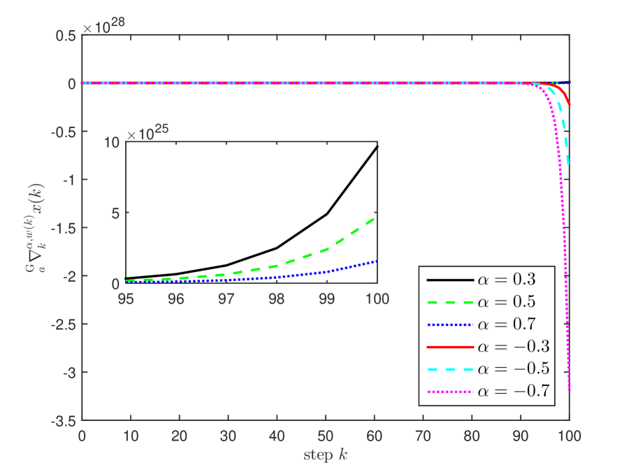
(a) $w(k)=0.5^{k-a}$

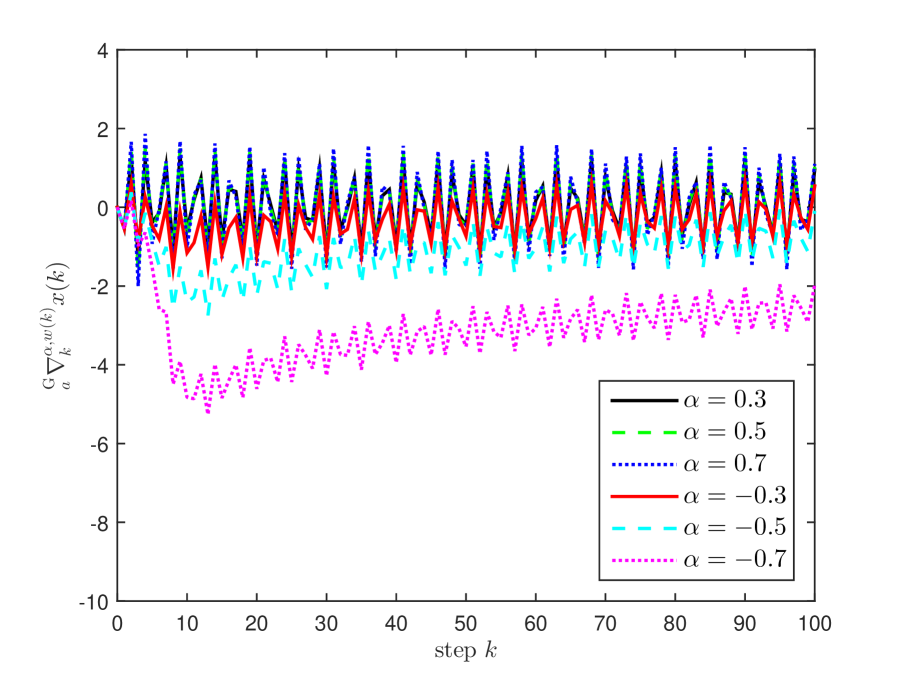
(b) $w(k)=0.5^{k-a}+0.01$

Figure 1: Time evolution of ${}_{a}^{\rm G}\nabla_{k}^{\alpha,w(k)}x(k)$.

To show more details, the following four cases are considered.

$$\left\{\begin{array}[]{l}{\rm{case}}\;1:\;w(k)={\sqrt{2}^{k-a}};\\ {\rm{case}}\;2:\;w(k)=-{\pi^{k-a}};\\ {\rm{case}}\;3:\;w(k)={(-1)^{k-a}};\\ {\rm{case}}\;4:\;w(k)=\sin(\frac{{k\pi}}{2}-\frac{{a\pi}}{2}+\frac{\pi}{4}).\end{array}\right.$$

The obtained results are shown as Fig. 2. In case 1, $w(k)$ is positive and monotonically increasing. In case 2, $w(k)$ is negative and monotonically decreasing. In case 3, $w(k)$ is in oscillation. Its positive value and negative value appear alternatively. In case 4, $w(k)$ is also in oscillation. Two positive value will appear after two negative value. It can be found that no matter for the fractional difference or the fractional sum, different $w(k)$ correspond to different ${}_{a}^{\rm G}\nabla_{k}^{\alpha,w(k)}x(k)$ in Fig. 2. To clear show the difference, setting case 1 as the standard, the error of ${}_{a}^{\rm G}\nabla_{k}^{\alpha,w(k)}x(k)$ between each case with the standard is calculated and displayed in Fig. 3. It is shown that the error always exists and cannot be ignored. Along this way, different tempered functions can be constructed for different scenarios and satisfied different demands, which could provide great potential to apply nabla tempered fractional calculus.

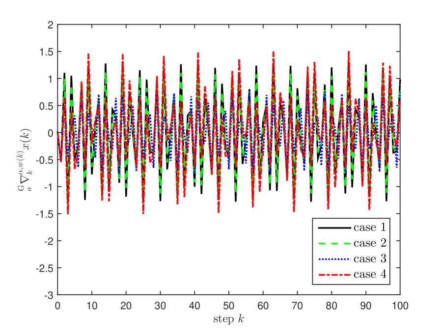
(a) $\alpha=0.5$

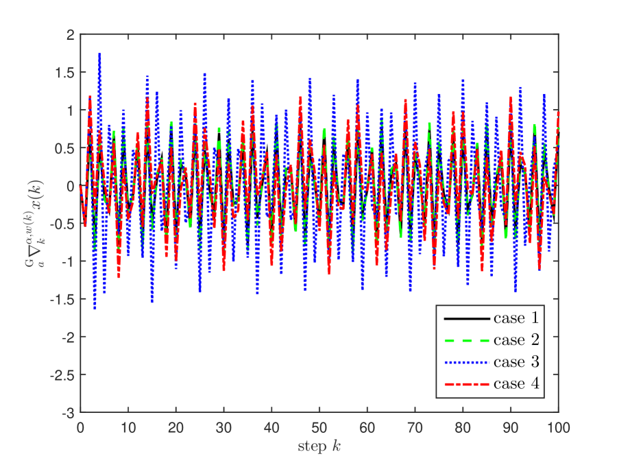
(b) $\alpha=-0.5$

Figure 2: Time evolution of ${}_{a}^{\rm G}\nabla_{k}^{\alpha,w(k)}x(k)$.

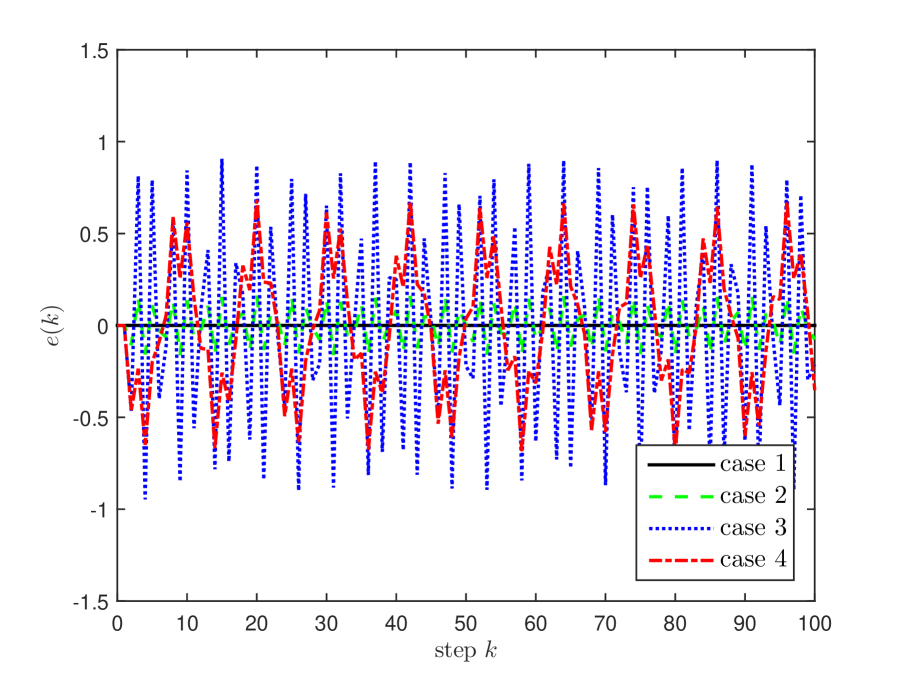
(a) $\alpha=0.5$

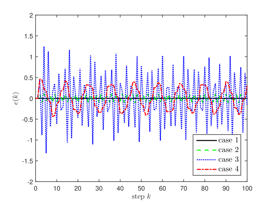
(b) $\alpha=-0.5$

Figure 3: The error of ${}_{a}^{\rm G}\nabla_{k}^{\alpha,w(k)}x(k)$ in different case.

To further check the value of tempered fractional difference, selecting $x(k)=\sin(10k)$, $\alpha=0.5$ and the above mentioned four cases, the results are shown as Fig. 4.

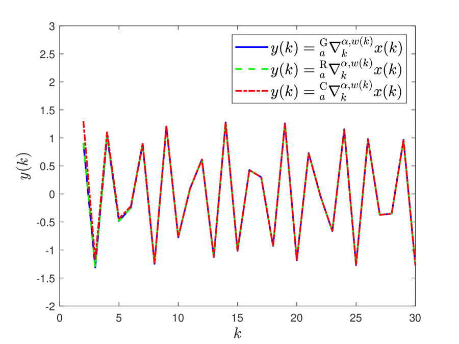
(a) $w(k)={\sqrt{2}^{k-a}}$

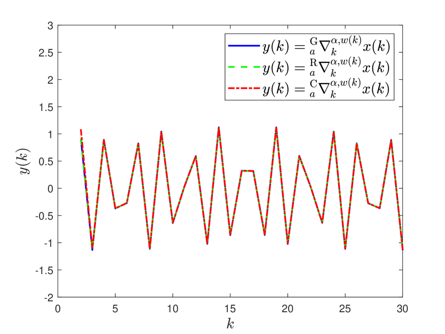
(b) $w(k)=-{\pi^{k-a}}$

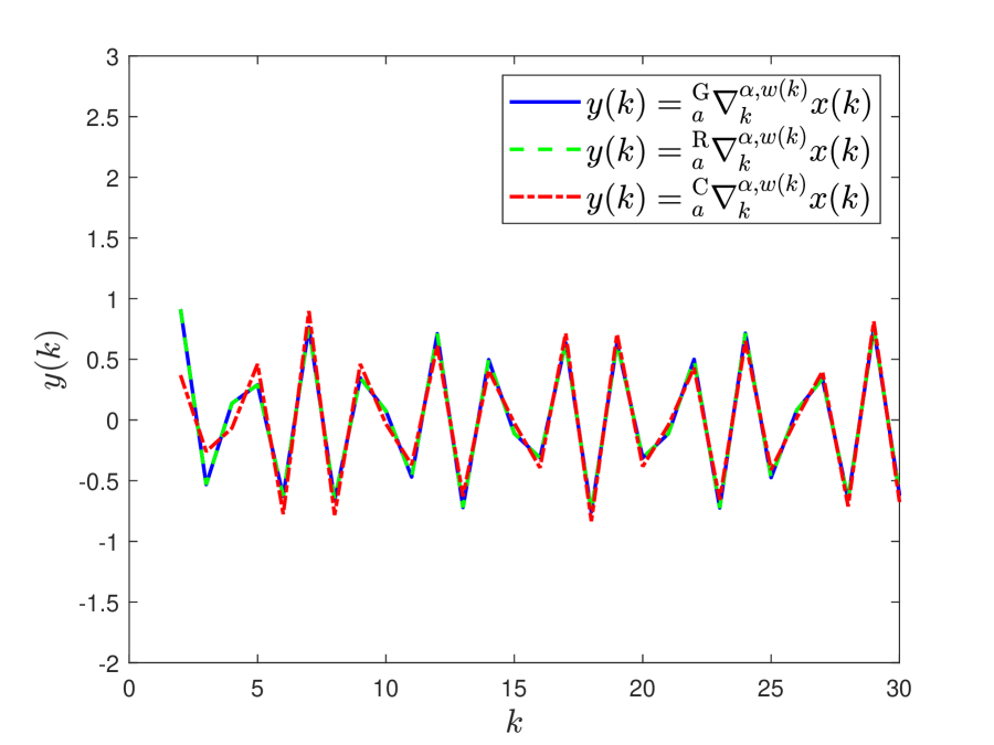
(c) $w(k)={(-1)^{k-a}}$

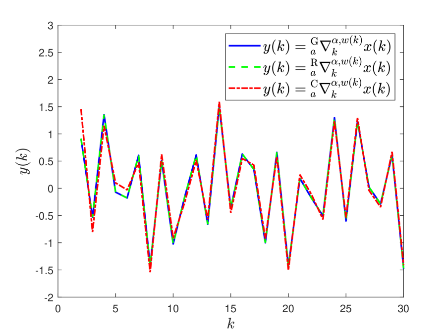
(d) $w(k)=\sin(\frac{{k\pi}}{2}-\frac{{a\pi}}{2}+\frac{\pi}{4})$

Figure 4: Time evolution of ${}_{a}^{\rm G}\nabla_{k}^{\alpha,w(k)}x(k)$, ${}_{a}^{\rm R}\nabla_{k}^{\alpha,w(k)}x(k)$ and ${}_{a}^{\rm C}\nabla_{k}^{\alpha,w(k)}x(k)$.

It can be observed that for each $w(k)$, the difference of the three fractional differences is small. From the quantitative analysis, one has

$$\left\{\begin{array}[]{l}{\rm{case}}\;1:\;-4.4409\times 10^{-16}\leq{}_{a}^{\rm{G}}\nabla_{k}^{\alpha,w(k)}x(k)-{}_{a}^{\rm{R}}\nabla_{k}^{\alpha,w(k)}x(k)\leq 1.1102\times 10^{-15};\\ {\rm{case}}\;2:\;-8.8818\times 10^{-16}\leq{}_{a}^{\rm{G}}\nabla_{k}^{\alpha,w(k)}x(k)-{}_{a}^{\rm{R}}\nabla_{k}^{\alpha,w(k)}x(k)\leq 3.3307\times 10^{-16};\\ {\rm{case}}\;3:\;-1.0131\times 10^{-16}\leq{}_{a}^{\rm{G}}\nabla_{k}^{\alpha,w(k)}x(k)-{}_{a}^{\rm{R}}\nabla_{k}^{\alpha,w(k)}x(k)\leq 4.9960\times 10^{-16};\\ {\rm{case}}\;4:\;-2.2204\times 10^{-16}\leq{}_{a}^{\rm{G}}\nabla_{k}^{\alpha,w(k)}x(k)-{}_{a}^{\rm{R}}\nabla_{k}^{\alpha,w(k)}x(k)\leq 4.4409\times 10^{-16},\end{array}\right.$$

which demonstrates the correctness of (16).

5 Conclusions

In this paper, the nabla tempered fractional difference and fractional sum have been investigated originally. A series of analytic properties are developed with rigorous mathematical proof including the equivalence relation, the nabla Taylor formula, and the nabla Laplace transform. It is believed that this work reveals the relationship between time domain and frequency domain of nabla tempered fractional calculus and enriches the knowledge of nabla tempered fractional calculus.

References

References

- Ceresa et al. [2022] I. Ceresa, D. Julián, F. Bonder, A Bourgain-Brezis-Mironescu formula for anisotropic fractional sobolev spaces and applications to anisotropic fractional differential equations, Journal of Mathematical Analysis and Applications 519 (2022) 126805.
- Arora et al. [2022] S. Arora, T. Mathur, S. Agarwal, K. Tiwari, P. Gupta, Applications of fractional calculus in computer vision: a survey, Neurocomputing 489 (2022) 407–428.
- Suzuki et al. [2022] J. Suzuki, M. Gulian, M. Zayernouri, D. Marta, Fractional modeling in action: a survey of nonlocal models for subsurface transport, turbulent flows, and anomalous materials, Journal of Peridynamics and Nonlocal Modeling (2022). Doi: 10.1007/s42102-022-00085-2.
- Reed et al. [2022] E. Reed, S. Chatterjee, G. Ramos, P. Bogdan, S. Pequito, Fractional cyber-neural systems - a brief survey, Annual Reviews in Control (2022). Doi: 10.1016/j.arcontrol.2022.06.002.
- Sabzikar et al. [2015] F. Sabzikar, M. M. Meerschaert, J. H. Chen, Tempered fractional calculus, Journal of Computational Physics 293 (2015) 14–28.
- Almeida and Morgado [2019] R. Almeida, M. L. Morgado, Analysis and numerical approximation of tempered fractional calculus of variations problems, Journal of Computational and Applied Mathematics 361 (2019) 1–12.
- Fernandez and Ustaoglu [2020] A. Fernandez, C. Ustaoglu, On some analytic properties of tempered fractional calculus, Journal of Computational and Applied Mathematics 366 (2020) 112400. Doi: 10.1016/j.cam.2019.112400.
- Mali et al. [2022] A. D. Mali, K. D. Kucche, A. Fernandez, H. M. Fahad, On tempered fractional calculus with respect to functions and the associated fractional differential equations, Mathematical Methods in the Applied Sciences 17 (2022) 12–27. Doi: 10.1002/mma.8441.
- Abdeljawad et al. [2020] T. Abdeljawad, S. Banerjee, G. C. Wu, Discrete tempered fractional calculus for new chaotic systems with short memory and image encryption, Optik 218 (2020) 163698. Doi: 10.1016/j.ijleo.2019.163698.
- Fu et al. [2021] H. Fu, L. L. Huang, T. Abdeljawad, C. Luo, Tempered fractional calculus on time scale for discrete-time systems, Fractals 29 (2021) 2140033. Doi: 10.1142/s0218348x21400338.
- Ferreira [2021] R. A. C. Ferreira, Discrete weighted fractional calculus and applications, Nonlinear Dynamics 104 (2021) 2531–2536.
- Cheng [2011] J. F. Cheng, Fractional Difference Equation Theory, Xiamen University Press, Xiamen, 2011.
- Ostalczyk [2015] P. Ostalczyk, Discrete Fractional Calculus: Applications in Control and Image Processing, World Scientific Publishing Company, Berlin, 2015.
- Goodrich and Peterson [2015] C. Goodrich, A. C. Peterson, Discrete Fractional Calculus, Springer, Cham, 2015.
- Ferreira [2022] R. A. C. Ferreira, Discrete Fractional Calculus and Fractional Difference Equations, Springer, Cham, 2022.
- Wei et al. [2019a] Y. H. Wei, W. D. Yin, Y. T. Zhao, Y. Wang, A new insight into the Grünwald–Letnikov discrete fractional calculus, Journal of Computational and Nonlinear Dynamics 14 (2019a) 041008–1:041008–5. Doi: 10.1115/1.4042635.
- Wei et al. [2019b] Y. H. Wei, Q. Gao, D. Y. Liu, Y. Wang, On the series representation of nabla discrete fractional calculus, Communications in Nonlinear Science and Numerical Simulation 69 (2019b) 198–218.
- Wei et al. [2019c] Y. H. Wei, Y. Q. Chen, Y. Wang, Y. Q. Chen, Some fundamental properties on the sampling free nabla Laplace transform, in: ASME 2019 International Design Engineering Technical Conferences Computers and Information in Engineering Conference, USA, Anaheim, 2019c. Doi: 10.1115/detc2019-97351.
- Atıcı et al. [2021] F. M. Atıcı, S. Chang, J. Jonnalagadda, Grünwald–Letnikov fractional operators: from past to present, Fractional Differential Calculus 11 (2021) 147–159.
- Li and Deng [2007] C. P. Li, W. H. Deng, Remarks on fractional derivatives, Applied Mathematics and Computation 187 (2007) 777–784.
- Almeida [2019] R. Almeida, Further properties of Osler’s generalized fractional integrals and derivatives with respect to another function, Rocky Mountain Journal of Mathematics 49 (2019) 2459–2493.
- Wei et al. [2021] Y. Q. Wei, D. Y. Liu, D. Boutat, H. R. Liu, Z. H. Wu, Modulating functions based model-free fractional order differentiators using a sliding integration window, Automatica 130 (2021) 109679. Doi: 10.1016/j.automatica.2021.109679.