Better Diffusion Models Further Improve Adversarial Training

Abstract

It has been recognized that the data generated by the denoising diffusion probabilistic model (DDPM) improves adversarial training. After two years of rapid development in diffusion models, a question naturally arises: can better diffusion models further improve adversarial training? This paper gives an affirmative answer by employing the most recent diffusion model (Karras et al., 2022) which has higher efficiency ($\sim 20$ sampling steps) and image quality (lower FID score) compared with DDPM. Our adversarially trained models achieve state-of-the-art performance on RobustBench using only generated data (no external datasets). Under the $\ell_{\infty}$-norm threat model with $\epsilon=8/255$, our models achieve $70.69\%$ and $42.67\%$ robust accuracy on CIFAR-10 and CIFAR-100, respectively, i.e. improving upon previous state-of-the-art models by $+4.58\%$ and $+8.03\%$. Under the $\ell_{2}$-norm threat model with $\epsilon=128/255$, our models achieve $84.86\%$ on CIFAR-10 ($+4.44\%$). These results also beat previous works that use external data. We also provide compelling results on the SVHN and TinyImageNet datasets. Our code is at https://github.com/wzekai99/DM-Improves-AT.

Table 1: A brief summary comparison of test accuracy (%) between our models and existing Rank #1 models, with (✓) and without (✗) external datasets, as listed in RobustBench (Croce et al., 2021). All of these models use the WRN-70-16 architecture.

Dataset	Method	External	Clean	AA
CIFAR-10 ($\ell_{\infty}$, $\epsilon=8/255$)	Rank #1	✗	88.74	66.11
		✓	92.23	66.58
	Ours	✗	93.25	70.69
CIFAR-10 ($\ell_{2}$, $\epsilon=128/255$)	Rank #1	✗	92.41	80.42
		✓	95.74	82.32
	Ours	✗	95.54	84.86
CIFAR-100 ($\ell_{\infty}$, $\epsilon=8/255$)	Rank #1	✗	63.56	34.64
		✓	69.15	36.88
	Ours	✗	75.22	42.67

1 Introduction

Adversarial training (AT) was first developed by Goodfellow et al. (2015), which has proven to be one of the most effective defenses against adversarial attacks (Madry et al., 2018; Zhang et al., 2019b; Rice et al., 2020) and dominated the winner solutions in adversarial competitions (Kurakin et al., 2018; Brendel et al., 2020). It is acknowledged that the availability of more data is critical to the performance of adversarially trained models (Schmidt et al., 2018; Stutz et al., 2019). Thus, several pioneer efforts are made to incorporate external datasets into AT (Hendrycks et al., 2019; Carmon et al., 2019; Alayrac et al., 2019; Najafi et al., 2019; Zhai et al., 2019; Wang et al., 2020), either in a fully-supervised or semi-supervised learning paradigm.

However, external datasets, even if unlabeled, are not always available. According to recent research, data generated by the denoising diffusion probabilistic model (DDPM) (Ho et al., 2020) can also significantly enhance both clean and robust accuracy of adversarially trained models, which is considered as a type of learning-based data augmentation (Rebuffi et al., 2021; Gowal et al., 2021; Rade & Moosavi-Dezfooli, 2021; Sehwag et al., 2022; Pang et al., 2022). Because of its effectiveness, on CIFAR-10 and CIFAR-100 (Krizhevsky & Hinton, 2009), the data generated by DDPM is used by all existing top-rank models (without external datasets) listed in RobustBench (Croce et al., 2021).

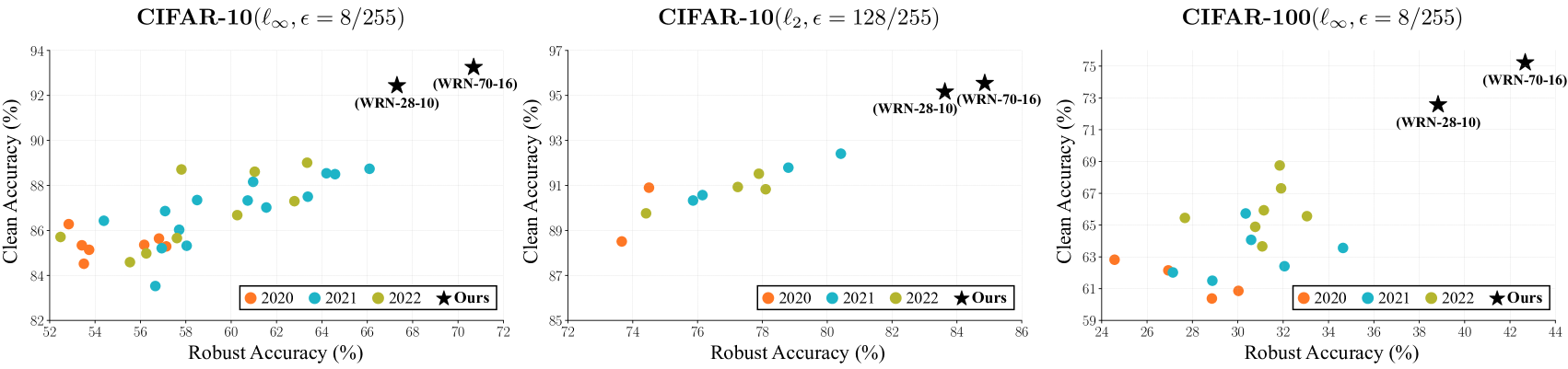
Figure 1: Robust accuracy (against AutoAttack) and clean accuracy of top-rank models (no external datasets) in the leaderboard of RobustBench. The publication year of top-rank models is indicated by different colors. Our models use the WRN-28-10 and WRN-70-16 architectures in each setting, and detailed accuracy values are provided in Table 2 and Table 3.

After two years of rapid development in diffusion models, many improvements in sampling quality and efficiency have been made beyond the initial work of DDPM (Song et al., 2021b). In particular, the elucidating diffusion model (EDM) (Karras et al., 2022) yields a new state-of-the-art (SOTA) FID score (Heusel et al., 2017) of $1.97$ in an unconditional setting, compared to DDPM’s FID score of $3.17$. While the images produced by DDPM and EDM are visually indistinguishable, we are curious whether better diffusion models (e.g., with lower FID scores) can benefit downstream applications even more (e.g., the task of AT).

It turns out that the reward for our curiosity is surprisingly good. We just replace the data generated by DDPM with the data generated by EDM and use almost the same training pipeline as described in Rebuffi et al. (2021). As summarized in Table 1, without the need for external datasets or additional training time per epoch, our adversarially trained WRN-70-16 models (Zagoruyko & Komodakis, 2016) achieve new SOTA robust accuracy on CIFAR-10/CIFAR-100 under AutoAttack (AA) (Croce & Hein, 2020), associated with a large improvement in clean accuracy. Our models even surpass previous Rank #1 models that rely on external data. The enhancements are significant enough—even our smaller model of WRN-28-10 architecture outperforms previous baselines, as shown in Figure 1. Our method can also substantially improve model performance on the SVHN and TinyImageNet datasets.

Moreover, we conduct extensive ablation studies to better reveal the mechanism by which diffusion models promote the AT process. Following the similar guidelines in Gowal et al. (2020) and Pang et al. (2021), we examine the effects of, e.g., quantity and quality of generated data, early stopping, and data augmentation. The results demonstrate that the data generated by EDM eliminates robust overfitting and reduces the generalization gap between clean and robust accuracy. During AT, we also conduct sensitivity analyses on a number of significant parameters. Our findings expand on the potential of learning-based data augmentation (i.e., using the data generated by diffusion models) and provide solid foundations for future research on promoting AT.

2 Related Work

Diffusion models. In recent years, denoising diffusion probabilistic modeling (Sohl-Dickstein et al., 2015; Ho et al., 2020) and score-based Langevin dynamics (Song & Ermon, 2019, 2020) have shown promising results in image generation. Song et al. (2021b) unify these two generative learning mechanisms using stochastic differential equations (SDE), and this unified model family is referred to as diffusion models. Later, there are emerging research routines that, to name a few, accelerate sampling inference (Song et al., 2021a; Lu et al., 2022), optimize model parametrization and sampling schedule (Kingma et al., 2021; Karras et al., 2022), and adopt diffusion models in text-to-image generation (Ramesh et al., 2022; Rombach et al., 2022).

Adversarial training. In addition to leveraging external datasets or generated data, several enhancements for AT have been made employing strategies inspired by other areas, including metric learning (Mao et al., 2019; Pang et al., 2020a, b), self-supervised learning (Chen et al., 2020a, b; Naseer et al., 2020; Wang & Liu, 2022), ensemble learning (Tramèr et al., 2018; Pang et al., 2019), fairness (Ma et al., 2022; Li & Liu, 2023), and generative modeling (Jiang et al., 2018; Wang & Yu, 2019; Deng et al., 2020). Xu & Liu (2022); Li et al. (2022); Zou & Liu (2023) study adversarial robust learning from the theoretical perspective. Moreover, because of high computational cost of AT, various attempts have been made to accelerate the training phase by reusing calculation (Shafahi et al., 2019; Zhang et al., 2019a) or one-step training (Wong et al., 2020; Liu et al., 2020; Vivek B & Venkatesh Babu, 2020). Some following studies address the side effects (e.g., catastrophic overfitting) induced by these fast AT approaches (Andriushchenko & Flammarion, 2020; Li et al., 2020).

Adversarial purification. Generative models have been used to purify adversarial examples (Song et al., 2018) or strengthen certified defenses (Carlini et al., 2022). Diffusion models have recently gained popularity in adversarial purification (Yoon et al., 2021; Nie et al., 2022; Wang et al., 2022; Xiao et al., 2022), demonstrating promising robust accuracy against AutoAttack. The effectiveness of diffusion-based purification, on the other hand, is dependent on the randomness of the SDE solvers (Ho et al., 2020; Bao et al., 2022), which causes at least tens of times inference computation and is unfriendly to downstream deployment. Furthermore, it has been demonstrated that stochastic pre-processing or test-time defenses have common limitations (Gao et al., 2022; Croce et al., 2022), which may be vulnerable to, e.g., transfer-based attacks (Kang et al., 2021) or intermediate-state attacks (Yang et al., 2022).

Adversarial benchmarks. Because of the large number of proposed defenses, it is critical to develop a comprehensive and up-to-date adversarial benchmark for ranking existing methods. Dong et al. (2020) perform large-scale experiments to generate robustness curves for evaluating typical defenses; Tang et al. (2021) provide comprehensive studies on how architecture design and training techniques affect robustness. Other benchmarks are available for specific scenarios, including adversarial patches (Hingun et al., 2022; Lian et al., 2022; Pintor et al., 2023), language-related tasks (Wang et al., 2021; Li et al., 2021), autonomous vehicles (Xu et al., 2022), multiple threat models (Hsiung et al., 2022), and common corruptions (Mu & Gilmer, 2019; Hendrycks & Dietterich, 2019; Sun et al., 2021). In this paper, we use RobustBench (Croce et al., 2021), which is a widely used benchmark in the community. RobustBench is built on AutoAttack, which has been proven to be reliable in evaluating deterministic defenses like adversarial training.

Table 2: Test accuracy (%) of clean images and under AutoAttack (AA) on CIFAR-10. We highlight our results in bold whenever the value represents an improvement relative to the strongest baseline using the same architecture, and we underline them whenever the value achieves new SOTA result under the threat model. We did not apply CutMix following Pang et al. (2022). ^†With the same batch size, the training time per epoch of our method is equivalent to the w/o-generated-data baseline (see ‘training time’ paragraph in Section 3).

Dataset	Architecture	Method	Generated	Batch	Epoch†	Clean	AA
CIFAR-10 ($\ell_{\infty}$, $\epsilon=8/255$)	WRN-34-20	Rice et al. (2020)	✗	128	200	85.34	53.42
	WRN-34-10	Zhang et al. (2020)	✗	128	120	84.52	53.51
	WRN-34-20	Pang et al. (2021)	✗	128	110	86.43	54.39
	WRN-34-10	Wu et al. (2020)	✗	128	200	85.36	56.17
	WRN-70-16	Gowal et al. (2020)	✗	512	200	85.29	57.14
	WRN-34-10	Sehwag et al. (2022)	10M	128	200	87.00	60.60
	WRN-28-10	Rebuffi et al. (2021)	1M	1024	800	87.33	60.73
		Pang et al. (2022)	1M	512	400	88.10	61.51
		Gowal et al. (2021)	100M	1024	2000	87.50	63.38
		Ours	1M	512	400	91.12	63.35
			1M	1024	800	91.43	63.96
			50M	2048	1600	92.27	67.17
			20M	2048	2400	92.44	67.31
	WRN-70-16	Pang et al. (2022)	1M	512	400	88.57	63.74
		Rebuffi et al. (2021)	1M	1024	800	88.54	64.20
		Gowal et al. (2021)	100M	1024	2000	88.74	66.11
		Ours	1M	512	400	91.98	65.54
			5M	512	800	92.58	67.92
			50M	1024	2000	93.25	70.69
CIFAR-10 ($\ell_{2}$, $\epsilon=128/255$)	WRN-34-10	Wu et al. (2020)	✗	128	200	88.51	73.66
	WRN-70-16	Gowal et al. (2020)	✗	512	200	90.9	74.50
	WRN-34-10	Sehwag et al. (2022)	10M	128	200	90.80	77.80
	WRN-28-10	Pang et al. (2022)	1M	512	400	90.83	78.10
		Rebuffi et al. (2021)	1M	1024	800	91.79	78.69
		Ours	1M	512	400	93.76	79.98
			50M	2048	1600	95.16	83.63
	WRN-70-16	Rebuffi et al. (2021)	1M	1024	800	92.41	80.42
		Ours	1M	512	400	94.47	81.16
			50M	1024	2000	95.54	84.86

3 Experiment Setup

We follow the basic setup and use the PyTorch implementation of Rebuffi et al. (2021). More information about the experimental settings can be found in Appendix A.

Model architectures. As our backbone networks, we adopt WideResNet (WRN) (Zagoruyko & Komodakis, 2016) with the Swish/SiLU activation function (Hendrycks & Gimpel, 2016). We use WRN-28-10 and WRN-70-16, the two most common architectures on RobustBench (Croce et al., 2021).

Generated data. To generate new images, we use the elucidating diffusion model (EDM) (Karras et al., 2022) that achieves SOTA FID scores. We employ the class-conditional EDM, whose training does not rely on external datasets (except for TinyImageNet, as specified in Section 4). We follow the guidelines in Carmon et al. (2019) to generate 1M CIFAR-10/CIFAR-100 images, which are selected from 5M generated images, with each image scored by a standardly pretrained WRN-28-10 model. We select the top $20\%$ scoring images for each class. When the amount of generated data exceeds 1M, or when generating data for SVHN/TinyImageNet, we adopt all generated images without selection. Note that unlike Rebuffi et al. (2021) and Gowal et al. (2021) that use unconditional DDPM, the pseudo-labels of the generated images are directly determined by the class conditioning in our implementation.

Training settings. We use TRADES (Zhang et al., 2019b) as the framework of adversarial training (AT), with $\beta=5$ for CIFAR-10/CIFAR-100, $\beta=6$ for SVHN, and $\beta=8$ for TinyImageNet. We adopt weight averaging with decay rate $\tau=0.995$ (Izmailov et al., 2018). We use the SGD optimizer with Nesterov momentum (Nesterov, 1983), where the momentum factor and weight decay are set to $0.9$ and $5\times 10^{-4}$, respectively. We use the cyclic learning rate schedule with cosine annealing (Smith & Topin, 2019), where the initial learning rate is set to $0.2$.

Training time. Regardless of the amount of generated data used (e.g., 1M, 20M, or 50M), the number of iterations per training epoch is controlled to be $\left\lceil{\frac{\textrm{amount of original data}}{\textrm{batch size}}}\right\rceil$ for all of our experiments utilizing generated data. This ensures a fair comparison with the w/o-generated-data baselines (e.g., those marked with ✗ in Table 2), as the training time remains constant when the number of training epochs and batch size are fixed. In particular, we sample images from the original and generated data in every training batch with a fixed ‘original-to-generated ratio’. Using CIFAR-10 (50K training images) and an original-to-generated ratio of 0.3, for example, each epoch involves training the model on 50K images: 15K from the original data and 35K from the generated data. For CIFAR-10/CIFAR-100 experiments, the original-to-generated ratio is $0.3$ for 1M generated data and $0.2$ when the required generated data exceeds 1M. Table 4 contains the original-to-generated ratios applied to SVHN and TinyImageNet, while Section B.1 contains additional ablation studies regarding the effects of different ratios.

Evaluation metrics. We evaluate model robustness against AutoAttack (Croce & Hein, 2020). Due to the high computation cost of AT, we cannot afford to report standard deviation for each experiment. For clarification, we train a WRN-28-10 model on CIFAR-10 with 1M generated data five times, using the batch size of $512$ and running for $400$ epochs. The clean accuracy is $91.12\pm 0.15\%$, and the robust accuracy under the $(\ell_{\infty},\epsilon=8/255)$ threat model is $63.35\pm 0.12\%$, indicating that our results have low variances.

Table 3: Test accuracy (%) of clean images and under AutoAttack (AA) on CIFAR-100. We highlight our results in bold whenever the value represents an improvement relative to the strongest baseline using the same architecture, and we underline them whenever the value achieves new SOTA result under the threat model. We did not apply CutMix following Pang et al. (2022). ^†With the same batch size, the training time per epoch of our method is equivalent to the w/o-generated-data baseline (see ‘training time’ paragraph in Section 3).

Dataset	Architecture	Method	Generated	Batch	Epoch†	Clean	AA
CIFAR-100 ($\ell_{\infty}$, $\epsilon=8/255$)	WRN-34-10	Wu et al. (2020)	✗	128	200	60.38	28.86
	WRN-70-16	Gowal et al. (2020)	✗	512	200	60.86	30.03
	WRN-34-10	Sehwag et al. (2022)	1M	128	200	65.90	31.20
	WRN-28-10	Pang et al. (2022)	1M	512	400	62.08	31.40
		Rebuffi et al. (2021)	1M	1024	800	62.41	32.06
		Ours	1M	512	400	68.06	35.65
			50M	2048	1600	72.58	38.83
	WRN-70-16	Pang et al. (2022)	1M	512	400	63.99	33.65
		Rebuffi et al. (2021)	1M	1024	800	63.56	34.64
		Ours	1M	512	400	70.21	38.69
			50M	1024	2000	75.22	42.67

Table 4: Test accuracy (%) of clean images and under AutoAttack (AA) on SVHN and TinyImageNet. We highlight the results following the notations in Table 3. Here ‘Ratio’ indicates the original-to-generated ratio. All the results adopt the WRN-28-10 model architecture. We did not apply CutMix following Pang et al. (2022). ^†Note that Gowal et al. (2021) utilize the class-conditional DDPM model on ImageNet (Dhariwal & Nichol, 2021) and directly generate images using the labels of TinyImageNet as the class condition.

Dataset	Method	Generated	Ratio	Batch	Epoch	Clean	AA
SVHN ($\ell_{\infty}$, $\epsilon=8/255$)	Gowal et al. (2021)	✗	✗	512	400	92.87	56.83
	Gowal et al. (2021)	1M	0.4	1024	800	94.15	60.90
	Rebuffi et al. (2021)	1M	0.4	1024	800	94.39	61.09
	Ours	1M	0.2	1024	800	95.19	61.85
		50M	0.2	2048	1600	95.56	64.01
TinyImageNet ($\ell_{\infty}$, $\epsilon=8/255$)	Gowal et al. (2021)	✗	✗	512	400	51.56	21.56
	Ours	1M	0.4	512	400	53.62	23.40
	Gowal et al. (2021)†	1M	0.3	1024	800	60.95	26.66
	Ours (ImageNet EDM)	1M	0.2	512	400	65.19	31.30

4 Comparison with State-of-the-Art

We compare our adversarially trained models with top-rank models in RobustBench that do not use external datasets. Table 2 shows the results under the ($\ell_{\infty}$, $\epsilon=8/255$) and ($\ell_{2}$, $\epsilon=128/255$) threat models on CIFAR-10; Tables 3 and 4 presents the results under the ($\ell_{\infty}$, $\epsilon=8/255$) threat model on CIFAR-100, SVHN, and TinyImageNet. In summary, previous top-rank models use images generated by DDPM, whereas our models use EDM and significantly improves both clean and robust accuracy. Our best models beat all RobustBench entries (including those that use external datasets) under these threat models.

Remark for Table 2. Under the ($\ell_{\infty}$, $\epsilon=8/255$) threat model on CIFAR-10, even when using 1M generated images, small batch size of $512$ and short training of $400$ epochs, our WRN-28-10 model achieves the robust accuracy comparable with Gowal et al. (2021) that use 100M generated images, while our clean accuracy improves significantly ($+3.62\%$). After applying a larger batch size of $2048$ and longer training of $2400$ epochs, our WRN-28-10 model surpasses the previous best result obtained by 100M generated data with a large margin (clean accuracy $+4.94\%$, robust accuracy $+3.93\%$), and even beats previous SOTA of WRN-70-16 model. When using 50M generated images and training for $2000$ epochs on WRN-70-16, our model reaches $93.25\%$ clean accuracy and $70.69\%$ robust accuracy, obtaining improvements of $+4.51\%$ and $+4.58\%$ over the SOTA result, respectively. This is the first adversarially trained model to achieve clean accuracy over $90\%$ and robust accuracy over $70\%$ without external datasets. Under the ($\ell_{2}$, $\epsilon=128/255$) threat model on CIFAR-10, our best WRN-28-10 model achieves $95.16\%$ ($+3.37\%$) clean accuracy and $83.63\%$ ($+4.94\%$) robust accuracy; our best WRN-70-16 model achieves $95.54\%$ ($+3.13\%$) clean accuracy and $84.86\%$ ($+4.44\%$) robust accuracy, which improve noticeably upon previous SOTA models.

Remark for Table 3. Using the images generated by EDM under the ($\ell_{\infty}$, $\epsilon=8/255$) threat model on CIFAR-100 results in surprisingly good performance. Specifically, our best WRN-28-10 model achieves $72.58\%$ ($+10.17\%$) clean accuracy and $38.83\%$ ($+6.77\%$) robust accuracy; our best WRN-70-16 model achieves $75.22\%$ ($+11.66\%$) clean accuracy and $42.67\%$ ($+8.03\%$) robust accuracy.

Remark for Table 4. We evaluate performance under the ($\ell_{\infty}$, $\epsilon=8/255$) threat model on SVHN and TinyImageNet datasets. As seen, our approach significantly outperforms the baselines. Our best model achieves $64.01\%$ ($+2.92\%$) robust accuracy on SVHN using 50M generated data.

We train the EDM model exclusively on TinyImageNet’s training set to produce 1M data. Our WRN-28-10 model obtains improvements of $+2.06\%$ and $+1.84\%$ over clean and robust accuracy, respectively. Notably, Gowal et al. (2021) utilize the class-conditional DDPM pre-trained on ImageNet (Dhariwal & Nichol, 2021) for data generation on TinyImagenet, since TinyImagenet dataset is a subset of ImageNet. To ensure a fair comparison, we use the checkpoint pre-trained on ImageNet provided by EDM, and class-conditional generate the images with the specific classes of TinyImageNet. The improvements are remarkable: our model achieves $65.19\%$ ($+4.24\%$) clean accuracy and $31.30\%$ ($+4.64\%$) robust accuracy with a smaller batch size and epoch than Gowal et al. (2021). These results demonstrate the effectiveness of generated data in enhancing model robustness across multiple datasets.

Table 5: Test accuracy (%) when training for different number of epochs, under the ($\ell_{\infty}$, $\epsilon=8/255$) threat model on CIFAR-10. WRN-28-10 models are trained with the batch size of $2048$ and original-to-generated ratio $0.2$. The model achieves the highest PGD-40 accuracy on the validation set at the ‘Best epoch’. ‘Early’ and ‘Last’ mean the test performance at the best and last epoch, respectively. ‘Diff’ denotes the accuracy gap between the ‘Early’ and ‘Last’.

Generated	Epoch	Best epoch	Clean				PGD-40				AA
			Early	Last	Diff		Early	Last	Diff		Early	Last	Diff
✗	400	86	84.41	82.18	$-$2.23		55.23	46.21	$-$9.02		54.57	44.89	$-$9.68
	800	88	83.60	82.15	$-$1.45		53.86	45.75	$-$8.11		53.13	44.58	$-$8.55
20M	400	370	91.27	91.45	$+$0.18		64.65	64.80	$+$0.15		63.69	63.84	$+$0.15
	800	755	92.08	92.14	$+$0.06		66.61	66.72	$+$0.11		65.66	65.63	$+$0.03
	1200	1154	92.43	92.32	$-$0.11		67.45	67.64	$+$0.19		66.31	66.60	$+$0.29
	1600	1593	92.51	92.61	$+$0.10		68.05	67.98	$-$0.07		67.14	67.10	$-$0.04
	2000	1978	92.41	92.55	$+$0.14		68.32	68.30	$-$0.02		67.22	67.17	$-$0.05
	2400	2358	92.58	92.54	$-$0.04		68.43	68.39	$-$0.04		67.31	67.30	$-$0.01

5 How Generated Data Influence Robustness

Rice et al. (2020) first observe the phenomenon of robust overfitting in AT: the test robust loss turns into increasing after a specific training epoch, e.g., shortly after the learning rate decay. The cause of robust overfitting is still debated (Pang et al., 2022), but one widely held belief is that the dataset is not large enough to achieve robust generalization (Schmidt et al., 2018). When the training set is dramatically expanded, using a large amount of external data (Carmon et al., 2019; Alayrac et al., 2019) or synthetic data (Gowal et al., 2021), significant improvements in both clean and robust accuracy are observed. In this section, we comprehensively study how the training details affect robust overfitting and model performance when generated images are applied to AT. Unless otherwise specified, the experiments are carried out on CIFAR-10 dataset and WRN-28-10 models that have been trained for $400$ epochs, with a batch size of $512$ and an original-to-generated ratio of $0.3$.

5.1 Early Stopping and Number of Epochs

In the standard setting, a line of research (Zhang et al., 2017; Belkin et al., 2019) has found that the deep learning model does not exhibit overfitting in practice, i.e., the testing loss decreases alongside the training loss and it is a common practice to train for as long as possible. For AT, however, Rice et al. (2020) reveal the phenomenon of robust overfitting: robust accuracy degrades rapidly on the test set while it continues to increase on the training set. A larger training epoch does not guarantee improved performance in the absence of generated data. Thus, early stopping becomes a default option in the AT process, which tracks the robust accuracy on a hold-out validation set and selects the checkpoint with the best validation robustness.

We conduct experiments on CIFAR-10 with 20M images generated by EDM to investigate how the training epoch and early stopping affect robust performance when sufficient images are used. The results are displayed in Table 5. We also provide results with no generated data for better comparison, and we can conclude that:

• Early stopping is effective when no generated data is used, as previously observed (Rice et al., 2020). Early stopping is triggered during the training process’s initial phase ($86$-th epoch/$400$ epochs; $88$-th epoch/$400$ epochs). On the test set, both clean and robust accuracy degrade, and longer training leads to poor performance.

• Early stopping is less important when using generated data. The best-performing model appears at the end of the training, implying that stopping early will not result in a significant improvement. ‘Diff’ becomes minor, indicating that adequate training data effectively mitigates robust overfitting.

• The model performs better with a longer training process when 20M generated images are used. Surprisingly, a short training epoch results in robust underfitting (‘Diff’ is positive). When the model is trained on enough data, the results suggest that training as long as possible benefits the robust performance.

We regard early stopping as a default trick consistent with previous works (Pang et al., 2021) because of its effectiveness on the original dataset and comparable performance on big data. Refer to Appendix A for implementation details.

Table 6: Test accuracy (%) when trained with different amounts of generated data, under the ($\ell_{\infty}$, $\epsilon=8/255$) threat model on CIFAR-10. The model achieves the highest PGD-40 accuracy on the validation set at the ‘Best epoch’. ‘Best’ is the highest accuracy ever achieved during training; ‘Last’ is the test performance at the last epoch. ‘Diff’ denotes the gap between ‘Best’ and ‘Last’. Since running AA is time-consuming, we regard AA accuracy at ‘Best epoch’ as the ‘Best’.

Generated	Best epoch	Clean				PGD-40				AA
		Best	Last	Diff		Best	Last	Diff		Best	Last	Diff
✗	91	84.55	82.59	$-$1.96		55.66	46.47	$-$9.19		54.37	45.29	$-$9.08
50K	171	86.15	85.47	$-$0.68		56.96	50.02	$-$6.94		55.71	48.85	$-$6.86
100K	274	88.20	87.47	$-$0.73		59.85	54.95	$-$4.90		58.85	53.42	$-$5.43
200K	365	89.71	89.48	$-$0.23		61.69	60.32	$-$1.37		59.91	59.11	$-$0.80
500K	395	90.76	90.58	$-$0.18		63.85	63.69	$-$0.16		62.76	62.77	$+$0.01
1M	394	91.13	90.89	$-$0.24		64.67	64.50	$-$0.17		63.35	63.50	$+$0.15
5M	395	91.15	90.93	$-$0.22		64.88	64.88	0		64.05	64.05	0
10M	396	91.25	91.18	$-$0.07		65.03	64.96	$-$0.07		64.19	64.28	$+$0.09
20M	399	91.17	91.07	$-$0.10		65.21	65.13	$-$0.08		64.27	64.16	$-$0.11
50M	395	91.24	91.15	$-$0.09		65.35	65.23	$-$0.12		64.53	64.51	$-$0.02

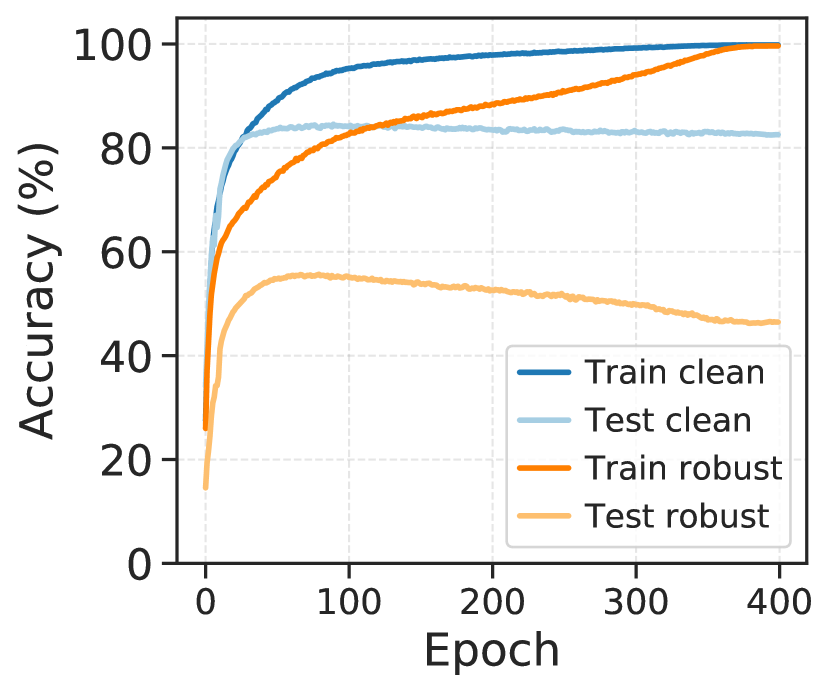
(a) no generated data

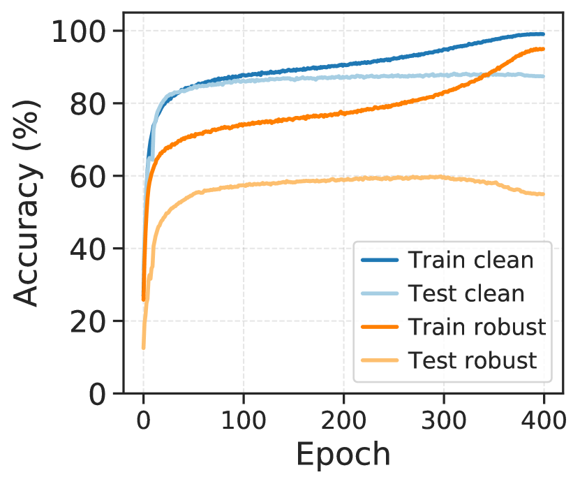
(b) 100K generated data

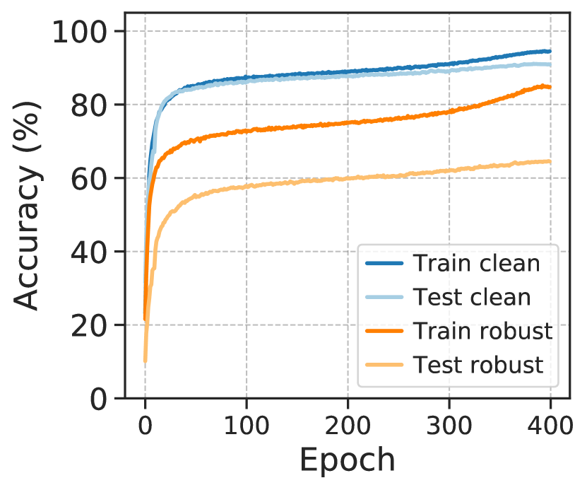
(c) 1M generated data

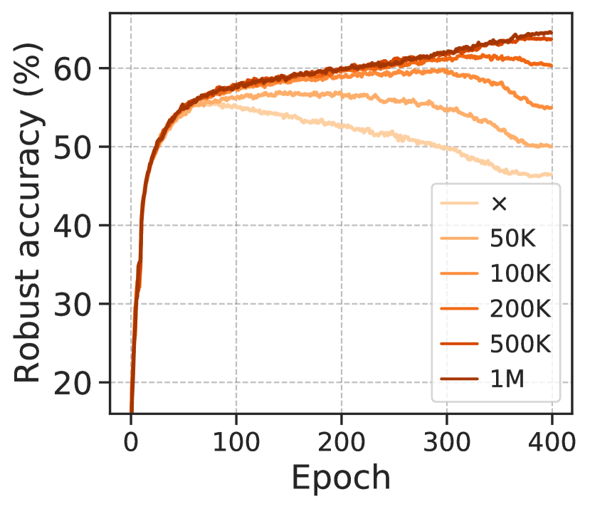
(d) effect of data amount

Figure 2: Clean and PGD robust accuracy of AT using (a) no generated data; (b) 100K generated data; (c) 1M generated data. (d) plots the PGD test robust accuracy of AT using different amounts of generated data.

5.2 Amount of Generated Data

We can sample many more images with the generated model than we could with the original training set. According to Gowal et al. (2021), more DDPM generated images result in a smaller robust generalization gap. Rebuffi et al. (2021) successfully prevent robust overfitting using DDPM to generate data of fixed size (1M), achieving stable performance after a drop in the learning rate. Here we look at how the size of the generated data affects robust overfitting. The results are displayed in Figure 2 and Table 6.

Figure 2 (a,b,c) depicts the clean and robust accuracy on the training and test sets in relation to different amounts of EDM generated data. More results with varying data sizes are shown in Section B.5. The findings indicate that:

• We can see a severe robust overfitting phenomenon when no generated data is used (Figure 2 (a), ‘✗’ in Table 6). After a certain epoch, the test clean accuracy degrades slightly, whereas the ‘Diff’ of robust accuracy is large. At the last epoch, the generalization gap between train and test robust accuracy is nearly $60\%$.

• Generated data can help to close the generalization gap for both clean and robust accuracy. In the final few epochs, without generated data, the training loss approaches zero. Train accuracy decreases as the size of the generated data increases, while test accuracy improves. The results show that the images generated by EDM contain those that are difficult to classify robustly, which benefits the robustness of model.

• The robust overfitting is alleviated with the increasing size of generated data, as shown in Figure 2 (d). After 500K generated images, the added generated images provide no significant improvement. In Table 6, ‘Diff’ after 500K generated images become minor and ‘Best epoch’ appears in the last few epochs. This is to be expected because the model’s capacity is insufficient to utilize all of the generated data. As a result, we provide SOTA results using a large model (WRN-70-16). A longer training epoch can also aid the model’s convergence on sufficient data, as seen in Table 5.

5.3 Data Augmentation

Data augmentation has been shown to improve standard training generalization by increasing the quantity and diversity of training data. It is somewhat surprising that almost all previous attempts to prevent robust overfitting solely through data augmentation have failed (Rice et al., 2020; Wu et al., 2020; Tack et al., 2022). Rebuffi et al. (2021) observe that combining data augmentation with weight averaging can promote robust accuracy, but it is less effective when using external data (e.g., 80M Tiny Images dataset). While Gowal et al. (2021) report that CutMix is compatible with using generated data, preliminary experiments in Pang et al. (2022) suggest that the effectiveness of CutMix may be dependent on the specific implementation.

To this end, we consider a variety of data augmentations and check their efficacy for AT with generated data. Common augmentation (He et al., 2016) is used in image classification tasks, including padding the image at each edge, cropping back to the original size, and horizontal flipping. Cutout (Devries & Taylor, 2017) randomly drops a region of the input image. CutMix (Yun et al., 2019) randomly replaces parts of an image with another. AutoAugment (Cubuk et al., 2019) and RandAugment (Cubuk et al., 2020) employ a combination of multiple image transformations such as Color, Rotation and Cutout to find the optimal composition. IDBH (Li & Spratling, 2023), the most recent augmentation scheme designed specifically for AT, achieves the best robust performance in the setting without additional data when compared to the augmentations mentioned above.

We consider common augmentation to be the baseline because it is the AT studies’ default setting. Using 1M EDM generated data, Table 7 demonstrates the performance of various data augmentations. No augmentation outperforms common augmentation in terms of robust accuracy (PGD-40 and AutoAttack). Cutout and IDBH outperform the other methods by a small margin. It should be noted that IDBH is intended for AT but also fails in the setting with generated data. In terms of clean accuracy, Cutout and AutoAugment slightly outperform common augmentation.

To summarize, rule-based (Cutout and CutMix) and policy-based (AutoAugment, RandAugment and IDBH) data augmentations appear to be less effective in improving robustness, particularly when using generated data. Our empirical findings contradict previous research, indicating that the efficacy of data augmentation for AT may be dependent on implementation. Thus, we use common augmentation as the default setting following Pang et al. (2022).

Table 7: Test accuracy (%) with different augmentation methods under the ($\ell_{\infty}$, $\epsilon=8/255$) threat model on CIFAR-10, using WRN-28-10 and 1M EDM generated data.

Methed	Clean	PGD-40	AA
Common	91.12	64.61	63.35
Cutout	91.25	64.54	63.30
CutMix	91.08	64.34	62.81
AutoAugment	91.23	64.07	62.86
RandAugment	91.14	64.39	63.12
IDBH	91.08	64.41	63.24

Table 8: Test accuracy (%) and FID with different sampling steps of diffusion model, under the ($\ell_{\infty}$, $\epsilon=8/255$) threat model on CIFAR-10, using WRN-28-10 and 1M EDM generated data. Here $\downarrow$ means ‘the lower the better’.

	Step	FID $\downarrow$	Clean	PGD-40	AA
Class-cond.	5	35.54	88.92	57.33	57.78
	10	2.477	90.96	66.21	62.81
	15	1.848	91.05	64.56	63.24
	20	1.824	91.12	64.61	63.35
	25	1.843	91.07	64.59	63.31
	30	1.861	91.10	64.51	63.25
	35	1.874	91.01	64.55	63.13
	40	1.883	91.03	64.44	63.03
Uncond.	5	37.78	88.00	56.92	57.19
	10	2.637	89.40	62.88	61.92
	15	1.998	89.36	63.47	62.31
	20	1.963	89.76	63.66	62.45
	25	1.977	89.61	63.63	62.40
	30	1.992	89.52	63.51	62.33
	35	2.003	89.39	63.56	62.37
	40	2.011	89.44	63.30	62.24

5.4 Quality of Generated Data

The number of sampling steps is a critical hyperparameter in diffusion models that controls generation quality and speed. Thus, we generate data with varying sampling steps in order to investigate how the quality of generated data affects model performance. We assess the quality by calculating the FID scores (Heusel et al., 2017) computed between 50K generated images and the original training images. In Section B.3, we investigate the effects of various samplers and EDM formulations on model robustness.

In supervised learning, there are unconditional and class-conditional paradigms for generative modeling. Extensive empirical evidence (Brock et al., 2019; Dhariwal & Nichol, 2021) demonstrates that class-conditional generative models are easier to train and have a lower FID than unconditional ones by leveraging data labels. We generate data in both class-conditional and unconditional settings, but give pseudo-labels in slightly different ways, to investigate the effect of class-conditioning on AT. For more information, please see Appendix A. We use EDM to generate 1M images, and the results are summarized in Table 8.

We find that low FID of generated data leads to high clean and robust accuracy. The results in Section B.3 come to the same conclusion. FID is a popular metric for comparing the distribution of generated images to the true distribution of data. Low FID indicates a small difference between the generated and true data distributions. The results show that we could increase the model’s robustness by bringing generated data closer to the true data.

Table 9: Test accuracy (%) with different values of batch size (left), label smoothing (LS) (middle), and $\beta$ in TRADES (right), under the ($\ell_{\infty}$, $\epsilon=8/255$) threat model on CIFAR-10.

Batch	Clean	PGD-40	AA
Size
128	91.12	64.77	63.90
256	91.15	65.76	64.72
512	91.81	66.15	65.21
1024	91.90	66.21	65.29
2048	91.98	66.54	65.50

LS	Clean	PGD-40	AA
0	90.40	64.32	62.83
0.1	91.12	64.61	63.35
0.2	91.23	64.38	63.27
0.3	91.06	64.35	63.12
0.4	90.82	64.15	62.87

$\beta$	Clean	PGD-40	AA
2	92.46	63.66	62.32
3	91.83	64.18	63.03
4	91.30	64.27	63.11
5	91.12	64.61	63.35
6	90.77	64.42	63.23
7	90.39	64.51	63.29
8	90.25	64.34	63.19

Class-conditional generation consistently outperforms unconditional generation, with lower FID and better robust performance. With $20$ sampling steps, both settings achieve the lowest FID and best performance. Thus, for the experiments on CIFAR-10, we use class-conditional generation with $20$ sampling steps and the checkpoint provided by EDM. The additional data for baselines in Section 4 is generated by DDPM, which has FID of $3.28$. On CIFAR-100/SVHN datasets, we train our own model and select the model with the best FID after $25$ sampling steps ($2.09$ for CIFAR-100, $1.39$ for SVHN, see Section B.2). In contrast, DDPM has FID of $5.58$ and $4.89$ on CIFAR-100 and SVHN, respectively (Gowal et al., 2021). The large promotion on FID provides a significant performance boost over the baselines in Section 4.

6 Sensitivity Analysis

In this section, we test the sensitivity of basic training hyperparameters on CIFAR-10. WRN-28-10 models are trained for $400$ epochs using 1M data generated by EDM. $512$ is the default batch size unless otherwise specified.

Batch size. In the standard setting, batch size is a crucial parameter that affects the performance of the model on large-scale datasets (Goyal et al., 2017). In the adversarial setting without external or generated data, the batch size is typically set to $128$ or $256$. Pang et al. (2021) investigate a wide range of batch sizes, from $64$ to $512$, and find that $128$ is optimal for CIFAR-10. To evaluate the effect of batch size on sufficient data, we train the model with 5M generated images and compare its performance across five different batch sizes in Section 5.4 (left). As observed, the largest batch size of $2048$ yields the best results. It implies that robust performance is enhanced by a large batch size when sufficient training data and a fixed initial learning rate are utilized. The optimal batch size may exist when the linear scaling rule is applied (Pang et al., 2021). A larger batch size requires additional GPU memory, but traverses the dataset more quickly. To achieve the best results in Section 4, we increase the batch size based on the model size and the number of GPUs in use. We choose $2048$ batch size for WRN-28-10 on $4\times$ A100 GPUs, and $1024$ batch size for WRN-70-16 on $8\times$ A100 GPUs.

Label smoothing. For standard training, label smoothing (LS) (Szegedy et al., 2016) improves standard generalization and alleviates the overconfidence problem (Hein et al., 2019), but it cannot prevent adaptive attacks from evading the model (Tramèr et al., 2020). In the adversarial setting, LS is used to prevent robust overfitting without external or generated data (Stutz et al., 2020; Chen et al., 2021). With 1M generated data, we evaluate the effect of LS on AT further. According to the results shown in Section 5.4 (middle), LS of $0.1$ improves both clean and robust accuracy (Clean $+0.72\%$, AA $+0.52\%$). LS of $0.2$ can further improve the clean accuracy by a small margin, but at the expense of robustness. Consistent with the findings of previous research (Jiang et al., 2020; Pang et al., 2021), excessive LS ($0.3$ and $0.4$) degrades the performance of the model. This is also the result of over-smoothing labels, which results in the loss of information in the output logits (Müller et al., 2019). We set $\textrm{LS}=0.1$ throughout the experiments for the best robust performance.

Effect of $\beta$. In the framework of TRADES (Zhang et al., 2019b), $\beta$ is an important hyperparameter that control the trade-off between robustness and accuracy (as in Eq. (2) of Appendix A). As the regularization parameter $\beta$ increases, the clean accuracy decreases while the robust accuracy increases, as observed by Zhang et al. (2019b). In contrast, when using 1M EDM generated data, the robustness of the model degrades with a large value of $\beta$. The best robustness is achieved with $\beta=5$ and smaller values of $\beta$ still contribute to improved clean accuracy. To provide the highest robust accuracy, $\beta=5$ is used on CIFAR-10/CIFAR-100. $\beta$ is set to $6$ and $8$ for SVHN and TinyImageNet, respectively.

7 Discussion

Diffusion models have proved their effectiveness in both adversarial training and adversarial purification; however, it is crucial to investigate how to more efficiently exploit diffusion models in the adversarial literature. For the time being, adversarial training requires millions of generated data even on small datasets such as CIFAR-10, which is inefficient in the training phase; adversarial purification requires tens of times forward processes through diffusion models, which is inefficient in the inference phase. Our work pushes the limits on the best performance of adversarially trained models, but there is still much to explore about the learning efficiency in the future research.

Appendix A Technical Details

Adversarial training. Let $\|\cdot\|_{p}$ denote $\ell_{p}$ norm, e.g., $\|\cdot\|_{2}$ and $\|\cdot\|_{\infty}$ denote the Euclidean norm $\ell_{2}$ and infinity norm $\ell_{\infty}$, respectively. $\mathcal{B}_{p}(x,\epsilon)\coloneqq\{x^{\prime}~{}|~{}\|x^{\prime}-x\|_{p}\leq\epsilon\}$ denotes that the input $x^{\prime}$ is constrained into the $\ell_{p}$ ball, where $\epsilon$ is the maximum perturbation constrain. Madry et al. (2018) formulate AT as a min-max optimization problem:

$$\operatorname*{arg\,min}_{\theta}\mathop{\mathbb{E}}\limits_{\begin{subarray}{c}(x,y)\sim\mathcal{D}\end{subarray}}\left[\max_{x^{\prime}\in\mathcal{B}_{p}(x,\epsilon)}\mathcal{L}(f_{\theta}(x^{\prime}),y)\right]\text{,}$$ (1)

where $\mathcal{D}$ is a data distribution over pairs of example $x$ and corresponding label $y$, $f_{\theta}(\cdot)$ is a neural network classifier with weights $\theta$, and $\mathcal{L}$ is the loss function. The inner optimization finds adversarial example $x^{\prime}$ that maximize the loss, while the outer optimization minimizes the loss on adversarial examples to update the network parameters $\theta$.

A typical variant of standard AT is TRADES (Zhang et al., 2019b), which is applied as our AT framework. The authors show that there exists a trade-off between clean and robust accuracy and decompose Eq. (1) into clean and robust objectives. TRADES combines these two objectives with a balancing hyperparameter to control such a trade-off:

$$\operatorname*{arg\,min}_{\theta}\mathop{\mathbb{E}}\limits_{\begin{subarray}{c}(x,y)\sim\mathcal{D}\end{subarray}}\left[\mathrm{CE}(f_{\theta}(x),y)+\beta\cdot\max_{x^{\prime}\in\mathcal{B}_{p}(x,\epsilon)}\mathrm{KL}(f_{\theta}(x)\|f_{\theta}(x^{\prime}))\right]\text{,}$$ (2)

where $\mathrm{CE}$ denotes the standard cross-entropy loss, $\mathrm{KL}(\cdot\|\cdot)$ denotes the Kullback–Leibler divergence, and $\beta$ is the hyperparameter to control the trade-off. In Section 6, we investigate the sensitivity of $\beta$ when generated data is used.

PGD attack. Projected gradient descent (PGD) (Madry et al., 2018) is a commonly used technique to solve the inner maximization problem in Eq. (1) and (2). Let $\operatorname{sign}(\bm{a})$ denote the sign of $\bm{a}$. $x_{0}$ is a randomly perturbed sample in the neighborhood $\mathcal{B}_{p}(x,\epsilon)$ of the clean input $x$, then PGD iteratively crafts the adversarial example for multiple gradient ascent steps $K$, formalized as:

$$x_{k}=\operatorname{clip}_{x,\epsilon}(x_{k-1}+\alpha\cdot\operatorname{sign}(\nabla_{x_{k-1}}\mathcal{L}(x_{k-1},y)))\text{,}$$ (3)

where $x_{k}$ denotes the adversarial example at step $k$, $\operatorname{clip}_{x,\epsilon}(x^{\prime})$ is the clipping function to project $x^{\prime}$ back into $\mathcal{B}_{p}(x,\epsilon)$, and $\alpha$ is the step size. We will refer to this inner optimization procedure with $K$ steps as PGD-$K$.

For adversary during AT, we apply PGD-10 attack with the following hyperparameters: for $\ell_{\infty}$ treat model, perturbation size $\epsilon=8/255$, step size $\alpha=2/255$ for CIFAR-10/CIFAR-100/TinyImageNet, and $\alpha=1.25/255$ for SVHN; for $\ell_{2}$ treat model, perturbation size $\epsilon=128/255$, step size $\alpha=32/255$ for CIFAR-10.

Generated data. Here we show more details about 1M images generation on CIFAR-10/CIFAR-100. For the unconditional generation, we use a pre-trained WRN-28-10 to give pseudo-labels, following Carmon et al. (2019); Rebuffi et al. (2021). The model is standardly trained on CIFAR-10 training set and achieves 96.15% test clean accuracy. For CIFAR-100, WRN-28-10 model achieves 80.47% test clean accuracy. Then we sample 5M images from unconditional EDM and score each image using the highest confidence provided by the pre-trained WRN-28-10 model. We regard the class which has the highest confidence as the pseudo-label. For each class, we select the top 100K scoring images for CIFAR-10 experiments (top 10K for CIFAR-100).

Slightly different from unconditional generating, class-conditional EDM can generate 1M samples belonging to a class directly; thus the pseudo-labels are directly determined by the class conditioning. For each class, we generate 500K and 50K images for CIFAR-10 and CIFAR-100 experiments, respectively. Similarly, we use the pre-trained WRN-28-10 model to score each image, and select the top 20% scoring images for each class.

When generating data for the SVHN and TinyImageNet datasets, or when the amount of generated data for CIFAR-10/CIFAR-100 exceeds 1M, we directly provide pseudo-labels using class-conditional generalization. Each class has an equal number of images to maintain data balance. The number of sampling steps is set to $20$ for CIFAR-10 (Section 5.4), $25$ for CIFAR-100/SVHN (Section B.2), and $40$ for TinyImageNet (following Karras et al. (2022)).

Datasets. CIFAR-10 and CIFAR-100 (Krizhevsky & Hinton, 2009) consist of 50K training images and 10K test images with 10 and 100 classes, respectively. All CIFAR images are 32$\times$32$\times$3 resolution (width, height, RGB channel). SVHN (Netzer et al., 2011) contains 73,257 training and 26,032 test images (0 $\sim$ 9 small cropped digits, 10 classes). TinyImageNet contains 100K images for training, and 10K images for testing. The images are 64$\times$64$\times$3 resolution with 200 classes.

More about setup. We utilize WideResNet (WRN) (Zagoruyko & Komodakis, 2016) following prior works (Madry et al., 2018; Rice et al., 2020; Rebuffi et al., 2021) which use variants of WRN family. Most experiments are conducted on WRN-28-10 (depth of 28, multiplier of 10) with 36M parameters. The experiments on WRN-28-10 are parallelly processed with four NVIDIA A100 SXM4 40GB GPUs. To evaluate how the abundant generated data affects large networks, we further use WRN-70-16 in Section 4, which contains 267M parameters. We use eight A100 GPUs to train WRN-70-16.

Following Rice et al. (2020) and discussion in Section 5, we perform early stopping as a defult trick. We separate first 1024 images of training set as a fixed validation set. During every epoch of AT, we pick the best checkpoint by evaluating robust accuracy under PGD-40 attack on the validation set.

Appendix B Additional Experiments

B.1 Original-to-Generated Ratio

Original-to-generated ratio is the mixing ratio between original and generated images in the training batch, e.g., a ratio of 0.3 indicates that for every 3 original images, we include 7 generated images. We investigate how the ratio affects the performance using 1M EDM generated data. We summarize the results in Figure 3. Both clean and robust accuracy achieve the best result with the ratio of 0.3. When the generated data is greater than 1M, we pick the ratio of 0.2 to achieve better performance (Table 10). We also observe that the performance of using 1M EDM generated data is better than using 50k original CIFAR-10 training set, consistent with Rebuffi et al. (2021). The results show that generated images improve the robustness as long as the generated model can produce high-quality data.

Figure 3: Clean accuracy and robust accuracy against PGD-40 and AA with respect to original-to-generated ratios (0 means generated images only, 1 means CIFAR-10 training set only). We train WRN-28-10 models against ($\ell_{\infty}$, $\epsilon=8/255$) on CIFAR-10 using 1M generated data.

Table 10: Test accuracy (%) against ($\ell_{\infty}$, $\epsilon=8/255$) on CIFAR-10 with different original-to-generated ratio. WRN-28-10 models are trained on 5M EDM generated data. The results of 0.2 are better than that of 0.3 consistently.

Batch	Epoch	Ratio	Clean	PGD-40	AA
512	400	0.2	91.15	64.97	64.25
		0.3	91.07	64.88	64.05
1024	800	0.2	91.87	66.43	65.53
		0.3	91.72	66.43	65.40
2048	1600	0.2	92.16	67.47	66.34
		0.3	91.88	67.19	66.29

B.2 FID for CIFAR-100 and SVHN datasets

We train our own EDM models to generate images for CIFAR-100 and SVHN experiments. The models are trained solely on CIFAR-100/SVHN training set. Table 11 shows the FID scores between generated data and CIFAR-100/SVHN training set with different sampling steps. The sampling step of 25 achieves the best FID.

Table 11: Fréchet inception distance (FID) between 50K EDM generated data and CIFAR-100/SVHN training set with different sampling steps of diffusion model.

Step	5	10	15	20	25	30	35	40
CIFAR-100	24.540	3.054	2.191	2.103	2.090	2.092	2.095	2.097
SVHN	125.765	5.458	1.661	1.405	1.393	1.410	1.428	1.445

B.3 Ablation Studies on the Specifics of Diffusion Model Implementation

We provide results on CIFAR-10 using various ODE samplers for diffusion models. We use the checkpoint for the unconditional diffusion model provided by Song et al. (2021b) and conduct ablation studies following Karras et al. (2022). Song et al. (2021b) employs Euler’s method on ODE sampler (i.e., DDIM solver, Line 1 in Section B.3 (left)), whereas Karras et al. (2022) discovered that Heun’s second-order method (i.e., EDM solver, Lines 2 and 3) yields superior results.

For the sake of a fair comparison, we employ double sampling steps for DDIM solver because it requires only half the time of EDM solver. Section B.3 (left) details the time required to generate 5M images, and 1M images are selected for training. Section B.3 (left) demonstrates that EDM solver improves FID significantly with the same generation time as DDIM solver; additionally, EDM solver promotes both clean and robust accuracy for adversarial training. The improved selection of EDM hyperparameters can further improve the robust performance of models.

We also provide results using variance preserving (VP) and variance exploding (VE) diffusion models, originally inspired by DDPM (Ho et al., 2020) and SMLD (Song & Ermon, 2019). In the implementation of EDM, the VP and VE models differ in their architecture, with DDPM++ and NCSN++ being utilized, respectively. We use VP formulation throughout the experiments in the main paper. Section B.3 (right) demonstrates that VE achieves a comparable FID to VP, consistent with previous findings (Karras et al., 2022). Both formulations result in similarly robust model performance.

Table 12: Test accuracy (%) with different samplers (left) and EDM formulations (right), under the ($\ell_{\infty}$, $\epsilon=8/255$) threat model on CIFAR-10. The sampling step is set to 20 in Table (right).

Sampler	Step	Time (h)	FID	Clean	PGD-40	AA
Song et al. (2021b)	40	3.75	10.06	86.97	61.49	60.53
+Heun & EDM $t_{i}$	20	3.62	4.03	87.82	62.17	61.29
+EDM $\sigma(t)$ & $s(t)$	20	3.62	2.98	88.09	62.36	61.46

	FID	Clean	PGD-40	AA
VP	1.824	91.12	64.61	63.35
VE	1.832	91.11	64.53	63.29

B.4 Computational Time

We provide the runtime for class-conditional and unconditional EDM generating 5M images with different sampling steps. The generation is processed with four A100 GPUs. As shown in Table 13, unconditional generation is faster than class-conditional one with a small margin, while resulting in lower robust performance (Table 8).

For adversarial training, WRN-28-10 and WRN-70-16 are parallelly processed with four and eight A100 GPUs, respectively. It takes 3.45 min on average to train one epoch on WRN-28-10 model with 2048 batch size. Training one epoch for WRN-70-16 model with 1024 batch size takes 9.93 min on average.

Table 13: Time (h) for class-conditional and unconditional EDM generating 5M data.

Step	5	10	15	20	25	30	35	40
Class-conditional	2.59	5.37	8.13	10.92	13.72	16.47	19.26	22.03
Unconditional	2.52	5.30	8.05	10.81	13.57	16.40	19.18	21.95

B.5 Amount of Generated Data

Figure 4 shows clean and PGD robust accuracy using different amounts of generated data. The robust overfitting is alleviated significantly as the size of generated data increases. After 500K generated images, the added generated images can not further close the generalization gap for both clean and robust accuracy. This is expected as the model capacity is too low to take advantage of all this generated data.

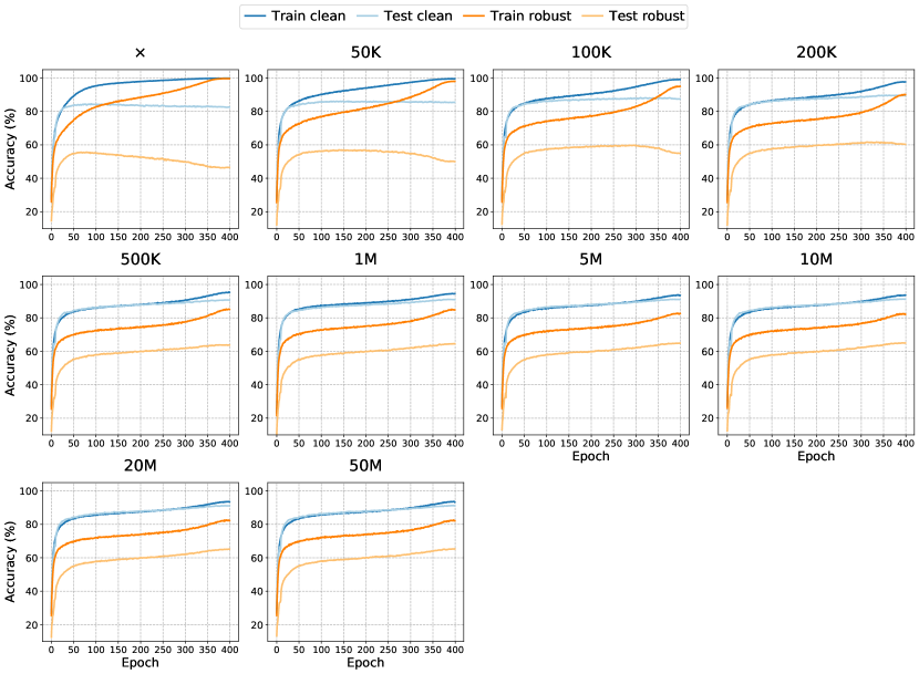
Figure 4: Clean and PGD robust accuracy of adversarial training using different amounts of generated data.

References

- Alayrac et al. (2019) Alayrac, J., Uesato, J., Huang, P., Fawzi, A., Stanforth, R., and Kohli, P. Are labels required for improving adversarial robustness? In Advances in Neural Information Processing Systems (NeurIPS), pp. 12192–12202, 2019.
- Andriushchenko & Flammarion (2020) Andriushchenko, M. and Flammarion, N. Understanding and improving fast adversarial training. In Advances in neural information processing systems (NeurIPS), 2020.
- Bao et al. (2022) Bao, F., Li, C., Zhu, J., and Zhang, B. Analytic-dpm: an analytic estimate of the optimal reverse variance in diffusion probabilistic models. In International Conference on Learning Representations (ICLR), 2022.
- Belkin et al. (2019) Belkin, M., Hsu, D., Ma, S., and Mandal, S. Reconciling modern machine-learning practice and the classical bias–variance trade-off. Proceedings of the National Academy of Sciences, 116(32):15849–15854, 2019.
- Brendel et al. (2020) Brendel, W., Rauber, J., Kurakin, A., Papernot, N., Veliqi, B., Mohanty, S. P., Laurent, F., Salathé, M., Bethge, M., Yu, Y., et al. Adversarial vision challenge. In The NeurIPS’18 Competition, pp. 129–153. Springer, 2020.
- Brock et al. (2019) Brock, A., Donahue, J., and Simonyan, K. Large scale GAN training for high fidelity natural image synthesis. In International Conference on Learning Representations (ICLR), 2019.
- Carlini et al. (2022) Carlini, N., Tramer, F., Kolter, J. Z., et al. (certified!!) adversarial robustness for free! arXiv preprint arXiv:2206.10550, 2022.
- Carmon et al. (2019) Carmon, Y., Raghunathan, A., Schmidt, L., Duchi, J. C., and Liang, P. Unlabeled data improves adversarial robustness. In Advances in Neural Information Processing Systems (NeurIPS), pp. 11190–11201, 2019.
- Chen et al. (2020a) Chen, K., Chen, Y., Zhou, H., Mao, X., Li, Y., He, Y., Xue, H., Zhang, W., and Yu, N. Self-supervised adversarial training. In IEEE International Conference on Acoustics, Speech and Signal Processing (ICASSP), pp. 2218–2222. IEEE, 2020a.
- Chen et al. (2020b) Chen, T., Liu, S., Chang, S., Cheng, Y., Amini, L., and Wang, Z. Adversarial robustness: From self-supervised pre-training to fine-tuning. In Conference on Computer Vision and Pattern Recognition (CVPR), pp. 699–708, 2020b.
- Chen et al. (2021) Chen, T., Zhang, Z., Liu, S., Chang, S., and Wang, Z. Robust overfitting may be mitigated by properly learned smoothening. In International Conference on Learning Representations (ICLR), 2021.
- Croce & Hein (2020) Croce, F. and Hein, M. Reliable evaluation of adversarial robustness with an ensemble of diverse parameter-free attacks. In International Conference on Machine Learning (ICML), volume 119, pp. 2206–2216, 2020.
- Croce et al. (2021) Croce, F., Andriushchenko, M., Sehwag, V., Debenedetti, E., Flammarion, N., Chiang, M., Mittal, P., and Hein, M. Robustbench: a standardized adversarial robustness benchmark. In Advances in Neural Information Processing Systems (NeurIPS), 2021.
- Croce et al. (2022) Croce, F., Gowal, S., Brunner, T., Shelhamer, E., Hein, M., and Cemgil, T. Evaluating the adversarial robustness of adaptive test-time defenses. In International Conference on Machine Learning (ICML), 2022.
- Cubuk et al. (2019) Cubuk, E. D., Zoph, B., Mané, D., Vasudevan, V., and Le, Q. V. Autoaugment: Learning augmentation strategies from data. In IEEE Conference on Computer Vision and Pattern Recognition (CVPR), pp. 113–123, 2019.
- Cubuk et al. (2020) Cubuk, E. D., Zoph, B., Shlens, J., and Le, Q. Randaugment: Practical automated data augmentation with a reduced search space. In Advances in Neural Information Processing Systems (NeurIPS), 2020.
- Deng et al. (2020) Deng, Z., Dong, Y., Pang, T., Su, H., and Zhu, J. Adversarial distributional training for robust deep learning. In Advances in Neural Information Processing Systems (NeurIPS), 2020.
- Devries & Taylor (2017) Devries, T. and Taylor, G. W. Improved regularization of convolutional neural networks with cutout. CoRR, abs/1708.04552, 2017.
- Dhariwal & Nichol (2021) Dhariwal, P. and Nichol, A. Q. Diffusion models beat gans on image synthesis. In Advances in Neural Information Processing Systems (NeurIPS), pp. 8780–8794, 2021.
- Dong et al. (2020) Dong, Y., Fu, Q.-A., Yang, X., Pang, T., Su, H., Xiao, Z., and Zhu, J. Benchmarking adversarial robustness on image classification. In IEEE Conference on Computer Vision and Pattern Recognition (CVPR), pp. 321–331, 2020.
- Gao et al. (2022) Gao, Y., Shumailov, I., Fawaz, K., and Papernot, N. On the limitations of stochastic pre-processing defenses. In Advances in Neural Information Processing Systems (NeurIPS), 2022.
- Goodfellow et al. (2015) Goodfellow, I. J., Shlens, J., and Szegedy, C. Explaining and harnessing adversarial examples. In International Conference on Learning Representations (ICLR), 2015.
- Gowal et al. (2020) Gowal, S., Qin, C., Uesato, J., Mann, T. A., and Kohli, P. Uncovering the limits of adversarial training against norm-bounded adversarial examples. CoRR, abs/2010.03593, 2020.
- Gowal et al. (2021) Gowal, S., Rebuffi, S., Wiles, O., Stimberg, F., Calian, D. A., and Mann, T. A. Improving robustness using generated data. In Advances in Neural Information Processing Systems (NeurIPS), pp. 4218–4233, 2021.
- Goyal et al. (2017) Goyal, P., Dollár, P., Girshick, R. B., Noordhuis, P., Wesolowski, L., Kyrola, A., Tulloch, A., Jia, Y., and He, K. Accurate, large minibatch SGD: training imagenet in 1 hour. CoRR, abs/1706.02677, 2017.
- He et al. (2016) He, K., Zhang, X., Ren, S., and Sun, J. Deep residual learning for image recognition. In IEEE Conference on Computer Vision and Pattern Recognition (CVPR), pp. 770–778, 2016.
- Hein et al. (2019) Hein, M., Andriushchenko, M., and Bitterwolf, J. Why relu networks yield high-confidence predictions far away from the training data and how to mitigate the problem. In IEEE Conference on Computer Vision and Pattern Recognition (CVPR), pp. 41–50, 2019.
- Hendrycks & Dietterich (2019) Hendrycks, D. and Dietterich, T. Benchmarking neural network robustness to common corruptions and perturbations. In International Conference on Learning Representations (ICLR), 2019.
- Hendrycks & Gimpel (2016) Hendrycks, D. and Gimpel, K. Gaussian error linear units (gelus). CoRR, abs/1606.08415, 2016.
- Hendrycks et al. (2019) Hendrycks, D., Lee, K., and Mazeika, M. Using pre-training can improve model robustness and uncertainty. In International Conference on Machine Learning (ICML), 2019.
- Heusel et al. (2017) Heusel, M., Ramsauer, H., Unterthiner, T., Nessler, B., and Hochreiter, S. Gans trained by a two time-scale update rule converge to a local nash equilibrium. In Advances in Neural Information Processing Systems (NeurIPS), pp. 6626–6637, 2017.
- Hingun et al. (2022) Hingun, N., Sitawarin, C., Li, J., and Wagner, D. Reap: A large-scale realistic adversarial patch benchmark. arXiv preprint arXiv:2212.05680, 2022.
- Ho et al. (2020) Ho, J., Jain, A., and Abbeel, P. Denoising diffusion probabilistic models. In Advances in Neural Information Processing Systems (NeurIPS), 2020.
- Hsiung et al. (2022) Hsiung, L., Tsai, Y.-Y., Chen, P.-Y., and Ho, T.-Y. Carben: Composite adversarial robustness benchmark. arXiv preprint arXiv:2207.07797, 2022.
- Izmailov et al. (2018) Izmailov, P., Podoprikhin, D., Garipov, T., Vetrov, D. P., and Wilson, A. G. Averaging weights leads to wider optima and better generalization. In Conference on Uncertainty in Artificial Intelligence (UAI), pp. 876–885, 2018.
- Jiang et al. (2018) Jiang, H., Chen, Z., Shi, Y., Dai, B., and Zhao, T. Learning to defense by learning to attack. arXiv preprint arXiv:1811.01213, 2018.
- Jiang et al. (2020) Jiang, L., Ma, X., Weng, Z., Bailey, J., and Jiang, Y. Imbalanced gradients: A new cause of overestimated adversarial robustness. CoRR, abs/2006.13726, 2020.
- Kang et al. (2021) Kang, Q., Song, Y., Ding, Q., and Tay, W. P. Stable neural ode with lyapunov-stable equilibrium points for defending against adversarial attacks. In Advances in Neural Information Processing Systems (NeurIPS), 2021.
- Karras et al. (2022) Karras, T., Aittala, M., Aila, T., and Laine, S. Elucidating the design space of diffusion-based generative models. In Advances in Neural Information Processing Systems (NeurIPS), 2022.
- Kingma et al. (2021) Kingma, D., Salimans, T., Poole, B., and Ho, J. Variational diffusion models. In Advances in Neural Information Processing Systems (NeurIPS), 2021.
- Krizhevsky & Hinton (2009) Krizhevsky, A. and Hinton, G. Learning multiple layers of features from tiny images. Technical report, Citeseer, 2009.
- Kurakin et al. (2018) Kurakin, A., Goodfellow, I., Bengio, S., Dong, Y., Liao, F., Liang, M., Pang, T., Zhu, J., Hu, X., Xie, C., et al. Adversarial attacks and defences competition. arXiv preprint arXiv:1804.00097, 2018.
- Li & Liu (2023) Li, B. and Liu, W. WAT: improve the worst-class robustness in adversarial training. In AAAI Conference on Artificial Intelligence (AAAI), 2023.
- Li et al. (2020) Li, B., Wang, S., Jana, S., and Carin, L. Towards understanding fast adversarial training. arXiv preprint arXiv:2006.03089, 2020.
- Li & Spratling (2023) Li, L. and Spratling, M. W. Data augmentation alone can improve adversarial training. In International Conference on Learning Representations (ICLR), 2023.
- Li et al. (2022) Li, X., Xin, Z., and Liu, W. Defending against adversarial attacks via neural dynamic system. In Advances in Neural Information Processing Systems (NeurIPS), 2022.
- Li et al. (2021) Li, Z., Xu, J., Zeng, J., Li, L., Zheng, X., Zhang, Q., Chang, K.-W., and Hsieh, C.-J. Searching for an effective defender: Benchmarking defense against adversarial word substitution. arXiv preprint arXiv:2108.12777, 2021.
- Lian et al. (2022) Lian, J., Mei, S., Zhang, S., and Ma, M. Benchmarking adversarial patch against aerial detection. IEEE Transactions on Geoscience and Remote Sensing, 60:1–16, 2022.
- Liu et al. (2020) Liu, G., Khalil, I., and Khreishah, A. Using single-step adversarial training to defend iterative adversarial examples. arXiv preprint arXiv:2002.09632, 2020.
- Lu et al. (2022) Lu, C., Zhou, Y., Bao, F., Chen, J., Li, C., and Zhu, J. Dpm-solver: A fast ode solver for diffusion probabilistic model sampling in around 10 steps. In Advances in Neural Information Processing Systems (NeurIPS), 2022.
- Ma et al. (2022) Ma, X., Wang, Z., and Liu, W. On the tradeoff between robustness and fairness. In Advances in Neural Information Processing Systems (NeurIPS), volume 35, pp. 26230–26241, 2022.
- Madry et al. (2018) Madry, A., Makelov, A., Schmidt, L., Tsipras, D., and Vladu, A. Towards deep learning models resistant to adversarial attacks. In International Conference on Learning Representations (ICLR), 2018.
- Mao et al. (2019) Mao, C., Zhong, Z., Yang, J., Vondrick, C., and Ray, B. Metric learning for adversarial robustness. In Advances in Neural Information Processing Systems (NeurIPS), 2019.
- Mu & Gilmer (2019) Mu, N. and Gilmer, J. Mnist-c: A robustness benchmark for computer vision. arXiv preprint arXiv:1906.02337, 2019.
- Müller et al. (2019) Müller, R., Kornblith, S., and Hinton, G. E. When does label smoothing help? In Advances in Neural Information Processing Systems (NeurIPS), pp. 4696–4705, 2019.
- Najafi et al. (2019) Najafi, A., Maeda, S.-i., Koyama, M., and Miyato, T. Robustness to adversarial perturbations in learning from incomplete data. In Advances in Neural Information Processing Systems (NeurIPS), 2019.
- Naseer et al. (2020) Naseer, M., Khan, S., Hayat, M., Khan, F. S., and Porikli, F. A self-supervised approach for adversarial robustness. In Conference on Computer Vision and Pattern Recognition (CVPR), 2020.
- Nesterov (1983) Nesterov, Y. E. A method for solving the convex programming problem with convergence rate . In Dokl. Akad. Nauk SSSR, volume 269, pp. 543–547, 1983.
- Netzer et al. (2011) Netzer, Y., Wang, T., Coates, A., Bissacco, A., Wu, B., and Ng, A. Reading digits in natural images with unsupervised feature learning. In NeurIPS Workshop on Deep Learning and Unsupervised Feature Learning, 2011.
- Nie et al. (2022) Nie, W., Guo, B., Huang, Y., Xiao, C., Vahdat, A., and Anandkumar, A. Diffusion models for adversarial purification. In International Conference on Machine Learning (ICML), 2022.
- Pang et al. (2019) Pang, T., Xu, K., Du, C., Chen, N., and Zhu, J. Improving adversarial robustness via promoting ensemble diversity. In International Conference on Machine Learning (ICML), 2019.
- Pang et al. (2020a) Pang, T., Xu, K., Dong, Y., Du, C., Chen, N., and Zhu, J. Rethinking softmax cross-entropy loss for adversarial robustness. In International Conference on Learning Representations (ICLR), 2020a.
- Pang et al. (2020b) Pang, T., Yang, X., Dong, Y., Xu, K., Su, H., and Zhu, J. Boosting adversarial training with hypersphere embedding. In Advances in Neural Information Processing Systems (NeurIPS), 2020b.
- Pang et al. (2021) Pang, T., Yang, X., Dong, Y., Su, H., and Zhu, J. Bag of tricks for adversarial training. In International Conference on Learning Representations (ICLR), 2021.
- Pang et al. (2022) Pang, T., Lin, M., Yang, X., Zhu, J., and Yan, S. Robustness and accuracy could be reconcilable by (proper) definition. In International Conference on Machine Learning (ICML), volume 162, pp. 17258–17277, 2022.
- Pintor et al. (2023) Pintor, M., Angioni, D., Sotgiu, A., Demetrio, L., Demontis, A., Biggio, B., and Roli, F. Imagenet-patch: A dataset for benchmarking machine learning robustness against adversarial patches. Pattern Recognition, 134:109064, 2023.
- Rade & Moosavi-Dezfooli (2021) Rade, R. and Moosavi-Dezfooli, S.-M. Helper-based adversarial training: Reducing excessive margin to achieve a better accuracy vs. robustness trade-off. In ICML 2021 Workshop on Adversarial Machine Learning, 2021.
- Ramesh et al. (2022) Ramesh, A., Dhariwal, P., Nichol, A., Chu, C., and Chen, M. Hierarchical text-conditional image generation with clip latents. arXiv preprint arXiv:2204.06125, 2022.
- Rebuffi et al. (2021) Rebuffi, S., Gowal, S., Calian, D. A., Stimberg, F., Wiles, O., and Mann, T. A. Fixing data augmentation to improve adversarial robustness. CoRR, abs/2103.01946, 2021.
- Rice et al. (2020) Rice, L., Wong, E., and Kolter, J. Z. Overfitting in adversarially robust deep learning. In International Conference on Machine Learning (ICML), 2020.
- Rombach et al. (2022) Rombach, R., Blattmann, A., Lorenz, D., Esser, P., and Ommer, B. High-resolution image synthesis with latent diffusion models. In IEEE Conference on Computer Vision and Pattern Recognition (CVPR), 2022.
- Schmidt et al. (2018) Schmidt, L., Santurkar, S., Tsipras, D., Talwar, K., and Madry, A. Adversarially robust generalization requires more data. In Advances in Neural Information Processing Systems (NeurIPS), pp. 5019–5031, 2018.
- Sehwag et al. (2022) Sehwag, V., Mahloujifar, S., Handina, T., Dai, S., Xiang, C., Chiang, M., and Mittal, P. Robust learning meets generative models: Can proxy distributions improve adversarial robustness? In International Conference on Learning Representations (ICLR), 2022.
- Shafahi et al. (2019) Shafahi, A., Najibi, M., Ghiasi, A., Xu, Z., Dickerson, J., Studer, C., Davis, L. S., Taylor, G., and Goldstein, T. Adversarial training for free! In Advances in Neural Information Processing Systems (NeurIPS), 2019.
- Smith & Topin (2019) Smith, L. N. and Topin, N. Super-convergence: Very fast training of neural networks using large learning rates. In Artificial intelligence and machine learning for multi-domain operations applications, volume 11006, pp. 369–386, 2019.
- Sohl-Dickstein et al. (2015) Sohl-Dickstein, J., Weiss, E., Maheswaranathan, N., and Ganguli, S. Deep unsupervised learning using nonequilibrium thermodynamics. In International Conference on Machine Learning (ICML), 2015.
- Song et al. (2021a) Song, J., Meng, C., and Ermon, S. Denoising diffusion implicit models. In International Conference on Learning Representations (ICLR), 2021a.
- Song & Ermon (2019) Song, Y. and Ermon, S. Generative modeling by estimating gradients of the data distribution. In Advances in Neural Information Processing Systems (NeurIPS), 2019.
- Song & Ermon (2020) Song, Y. and Ermon, S. Improved techniques for training score-based generative models. In Advances in Neural Information Processing Systems (NeurIPS), 2020.
- Song et al. (2018) Song, Y., Kim, T., Nowozin, S., Ermon, S., and Kushman, N. Pixeldefend: Leveraging generative models to understand and defend against adversarial examples. In International Conference on Learning Representations (ICLR), 2018.
- Song et al. (2021b) Song, Y., Sohl-Dickstein, J., Kingma, D. P., Kumar, A., Ermon, S., and Poole, B. Score-based generative modeling through stochastic differential equations. In International Conference on Learning Representations (ICLR), 2021b.
- Stutz et al. (2019) Stutz, D., Hein, M., and Schiele, B. Disentangling adversarial robustness and generalization. In IEEE Conference on Computer Vision and Pattern Recognition (CVPR), 2019.
- Stutz et al. (2020) Stutz, D., Hein, M., and Schiele, B. Confidence-calibrated adversarial training: Generalizing to unseen attacks. In International Conference on Machine Learning (ICML), volume 119, pp. 9155–9166, 2020.
- Sun et al. (2021) Sun, J., Mehra, A., Kailkhura, B., Chen, P.-Y., Hendrycks, D., Hamm, J., and Mao, Z. M. Certified adversarial defenses meet out-of-distribution corruptions: Benchmarking robustness and simple baselines. arXiv preprint arXiv:2112.00659, 2021.
- Szegedy et al. (2016) Szegedy, C., Vanhoucke, V., Ioffe, S., Shlens, J., and Wojna, Z. Rethinking the inception architecture for computer vision. In IEEE Conference on Computer Vision and Pattern Recognition (CVPR), pp. 2818–2826, 2016.
- Tack et al. (2022) Tack, J., Yu, S., Jeong, J., Kim, M., Hwang, S. J., and Shin, J. Consistency regularization for adversarial robustness. In AAAI Conference on Artificial Intelligence (AAAI), pp. 8414–8422, 2022.
- Tang et al. (2021) Tang, S., Gong, R., Wang, Y., Liu, A., Wang, J., Chen, X., Yu, F., Liu, X., Song, D., Yuille, A., et al. Robustart: Benchmarking robustness on architecture design and training techniques. arXiv preprint arXiv:2109.05211, 2021.
- Tramèr et al. (2018) Tramèr, F., Kurakin, A., Papernot, N., Boneh, D., and McDaniel, P. Ensemble adversarial training: Attacks and defenses. In International Conference on Learning Representations (ICLR), 2018.
- Tramèr et al. (2020) Tramèr, F., Carlini, N., Brendel, W., and Madry, A. On adaptive attacks to adversarial example defenses. In Advances in Neural Information Processing Systems (NeurIPS), 2020.
- Vivek B & Venkatesh Babu (2020) Vivek B, S. and Venkatesh Babu, R. Single-step adversarial training with dropout scheduling. In IEEE Conference on Computer Vision and Pattern Recognition (CVPR), 2020.
- Wang et al. (2021) Wang, B., Xu, C., Wang, S., Gan, Z., Cheng, Y., Gao, J., Awadallah, A. H., and Li, B. Adversarial glue: A multi-task benchmark for robustness evaluation of language models. arXiv preprint arXiv:2111.02840, 2021.
- Wang & Yu (2019) Wang, H. and Yu, C.-N. A direct approach to robust deep learning using adversarial networks. In International Conference on Learning Representations (ICLR), 2019.
- Wang et al. (2022) Wang, J., Lyu, Z., Lin, D., Dai, B., and Fu, H. Guided diffusion model for adversarial purification. arXiv preprint arXiv:2205.14969, 2022.
- Wang et al. (2020) Wang, Y., Zou, D., Yi, J., Bailey, J., Ma, X., and Gu, Q. Improving adversarial robustness requires revisiting misclassified examples. In International Conference on Learning Representations (ICLR), 2020.
- Wang & Liu (2022) Wang, Z. and Liu, W. Robustness verification for contrastive learning. In International Conference on Machine Learning (ICML), volume 162, pp. 22865–22883, 2022.
- Wong et al. (2020) Wong, E., Rice, L., and Kolter, J. Z. Fast is better than free: Revisiting adversarial training. In International Conference on Learning Representations (ICLR), 2020.
- Wu et al. (2020) Wu, D., Xia, S., and Wang, Y. Adversarial weight perturbation helps robust generalization. In Advances in Neural Information Processing Systems (NeurIPS), 2020.
- Xiao et al. (2022) Xiao, C., Chen, Z., Jin, K., Wang, J., Nie, W., Liu, M., Anandkumar, A., Li, B., and Song, D. Densepure: Understanding diffusion models towards adversarial robustness. arXiv preprint arXiv:2211.00322, 2022.
- Xu et al. (2022) Xu, C., Ding, W., Lyu, W., Liu, Z., Wang, S., He, Y., Hu, H., Zhao, D., and Li, B. Safebench: A benchmarking platform for safety evaluation of autonomous vehicles. In Advances in Neural Information Processing Systems (NeurIPS) Datasets and Benchmarks Track, 2022.
- Xu & Liu (2022) Xu, J. and Liu, W. On robust multiclass learnability. In Advances in Neural Information Processing Systems (NeurIPS), 2022.
- Yang et al. (2022) Yang, Z., Pang, T., and Liu, Y. A closer look at the adversarial robustness of deep equilibrium models. In Advances in Neural Information Processing Systems (NeurIPS), 2022.
- Yoon et al. (2021) Yoon, J., Hwang, S. J., and Lee, J. Adversarial purification with score-based generative models. In International Conference on Machine Learning (ICML), 2021.
- Yun et al. (2019) Yun, S., Han, D., Chun, S., Oh, S. J., Yoo, Y., and Choe, J. Cutmix: Regularization strategy to train strong classifiers with localizable features. In International Conference on Computer Vision (ICCV), pp. 6022–6031, 2019.
- Zagoruyko & Komodakis (2016) Zagoruyko, S. and Komodakis, N. Wide residual networks. In British Machine Vision Conference (BMVC), 2016.
- Zhai et al. (2019) Zhai, R., Cai, T., He, D., Dan, C., He, K., Hopcroft, J., and Wang, L. Adversarially robust generalization just requires more unlabeled data. arXiv preprint arXiv:1906.00555, 2019.
- Zhang et al. (2017) Zhang, C., Bengio, S., Hardt, M., Recht, B., and Vinyals, O. Understanding deep learning requires rethinking generalization. In International Conference on Learning Representations (ICLR), 2017.
- Zhang et al. (2019a) Zhang, D., Zhang, T., Lu, Y., Zhu, Z., and Dong, B. You only propagate once: Accelerating adversarial training via maximal principle. In Advances in Neural Information Processing Systems (NeurIPS), 2019a.
- Zhang et al. (2019b) Zhang, H., Yu, Y., Jiao, J., Xing, E. P., Ghaoui, L. E., and Jordan, M. I. Theoretically principled trade-off between robustness and accuracy. In International Conference on Machine Learning (ICML), volume 97, pp. 7472–7482, 2019b.
- Zhang et al. (2020) Zhang, J., Xu, X., Han, B., Niu, G., Cui, L., Sugiyama, M., and Kankanhalli, M. S. Attacks which do not kill training make adversarial learning stronger. In International Conference on Machine Learning (ICML), volume 119, pp. 11278–11287, 2020.
- Zou & Liu (2023) Zou, X. and Liu, W. Generalization bounds for adversarial contrastive learning. Journal of Machine Learning Research, 24(114):1–54, 2023.