Robust Question Answering against Distribution Shifts with
Test-Time Adaptation: An Empirical Study

Abstract

A deployed question answering (QA) model can easily fail when the test data has a distribution shift compared to the training data. Robustness tuning (RT) methods have been widely studied to enhance model robustness against distribution shifts before model deployment. However, can we improve a model after deployment? To answer this question, we evaluate test-time adaptation (TTA) to improve a model after deployment. We first introduce ColdQA, a unified evaluation benchmark for robust QA against text corruption and changes in language and domain. We then evaluate previous TTA methods on ColdQA and compare them to RT methods. We also propose a novel TTA method called online imitation learning (OIL). Through extensive experiments, we find that TTA is comparable to RT methods, and applying TTA after RT can significantly boost the performance on ColdQA. Our proposed OIL improves TTA to be more robust to variation in hyper-parameters and test distributions over time.

1 Introduction

How to build a trustworthy NLP system that is robust to distribution shifts is important, since the real world is changing dynamically and a system can easily fail when the test data has a distribution shift compared to the training data Ribeiro et al. (2020); Wang et al. (2022). Much previous work on robustness evaluation has found model failures on shifted test data. For example, question answering (QA) models are brittle when dealing with paraphrased questions Gan and Ng (2019), models for task-oriented dialogues fail to understand corrupted input Liu et al. (2021a); Peng et al. (2021), and neural machine translation degrades on noisy text input Belinkov and Bisk (2018). In this work, we study the robustness of QA models to out-of-distribution (OOD) test-time data.

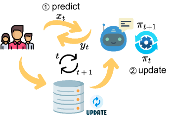
Figure 1: Illustration of test-time adaptation. $\pi$ represents the model being adapted. $x_{t}$ is the test data at time $t$ and $y_{t}$ is the returned predictions for $x_{t}$.

To build a model that is robust against distribution shifts, most previous work focuses on robustness tuning (RT) methods that improve model generalization pre-deployment, such as adversarial training Madry et al. (2018). However, can we continually enhance a model post-deployment? To answer this question, we study and evaluate test-time adaptation (TTA) for robust QA after model deployment. TTA generalizes a model by continually updating the model with test-time data Sun et al. (2020). As shown in Fig. 1, in this work, we focus on test-time adaptation in real time, where the model predicts and updates over a data stream on the fly. For each test data instance, the model first returns its prediction and then updates itself with the test data. Unlike unsupervised domain adaptation Ramponi and Plank (2020) studied in NLP, TTA is suitable for domain generalization, since it makes no assumption about the target distribution and could adapt the model to any arbitrary distribution at test time.

We discuss TTA methods in $\S$3, where we first present previous popular TTA baselines, and then introduce our newly proposed TTA method, online imitation learning (OIL). OIL is inspired by imitation learning, where the adapted model learns to clone the actions made by the source model, and the source model aims to reduce overfitting to noisy pseudo-labels in the adapted model. We further adopt causal inference to control model bias from the source model. Next, to compare to TTA methods, we briefly discuss previous robustness tuning (RT) methods such as adversarial training in $\S$4.

To study and analyze TTA for robust QA post-deployment, we introduce ColdQA in $\S$5 which is a unified evaluation benchmark for robust QA against distribution shifts from text corruption, language change, and domain change. It differs from previous benchmarks that only study one type of distribution shifts Ravichander et al. (2021); Hu et al. (2020); Fisch et al. (2019). ColdQA expects a QA model to generalize well to all three types of distribution shifts.

Our contributions in this work include:

• We are the first to study test-time adaptation for QA tasks with extensive experiments.

• We propose a novel TTA method, OIL, which outperforms previous TTA baselines.

• We propose a new benchmark ColdQA which unifies the evaluation of robust QA against distribution shifts.

• We evaluate previous robustness tuning methods on the new benchmark.

Based on the experimental results in $\S$6, we report the following findings:

• ColdQA is challenging and not all RT methods are effective on ColdQA ($\S$6.2);

• Overall, as Fig. 2 shows, TTA is comparable to RT, and applying TTA after RT can further boost model performance ($\S$6.2);

• Compared to previous TTA baselines, OIL is more robust to changes in hyper-parameters and test distributions over time ($\S$6.3).

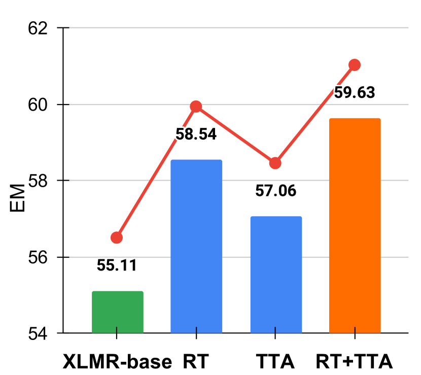
Figure 2: The average results of RT, TTA, and RT+TTA on ColdQA. RT+TTA significantly improves over RT and TTA.

Settings	Trianing Data		Training Loss
	Training time	Test time	Training time	Test time
Unsupervised domain adaptation	$\mathcal{X}^{s}$, $\mathcal{Y}^{s}$; $\mathcal{X}^{t}$	None	$\mathcal{L}(x_{s},y_{s})+\mathcal{L}(x_{t})$	None
Robustness tuning	$\mathcal{X}^{s}$, $\mathcal{Y}^{s}$	None	$\mathcal{L}(x^{s},y^{s})$	None
Test-time adaptation (online)	$\mathcal{X}^{s}$, $\mathcal{Y}^{s}$	$\mathcal{X}^{t}$	None	$\mathcal{L}(x^{t})$

Table 1: Compared settings. $\mathcal{X}^{s}$ and $\mathcal{Y}^{s}$ are drawn from a source distribution and $\mathcal{X}^{t}$ from a target distribution. $x^{s}\in\mathcal{X}^{s}$, $y^{s}\in\mathcal{Y}^{s}$, $x^{t}\in\mathcal{X}^{t}$.

2 Related Work

Robust QA   Much previous work on model robustness evaluation has shown that NLP models fail on test data with distribution shifts Rychalska et al. (2019); Ribeiro et al. (2020); Wang et al. (2022) compared to the training data. For QA tasks, Ravichander et al. (2021) study how text corruption affects QA performance. Lewis et al. (2020) and Artetxe et al. (2020) analyze cross-lingual transfer of a QA system. Fisch et al. (2019) benchmark the generalization of QA models to data with domain shift. In this work, we jointly study distribution shifts due to corruption, language change, and domain change. Adversarial samples cause another type of distribution shifts Jia and Liang (2017) which is not studied in this work. Hard samples Ye et al. (2022), dataset bias Tu et al. (2020), and other robustness issues are not the focus of this work.

Test-Time Adaptation   TTA adapts a source model with test-time data from a target distribution. TTA has been verified to be very effective in image recognition Sun et al. (2020); Wang et al. (2021b); Liu et al. (2021b); Bartler et al. (2022). In NLP, Wang et al. (2021d) learn to combine adapters on low-resource languages at test time to improve sequence labeling tasks. Gao et al. (2022) and Li et al. (2022) keep adapting a QA model after model deployment using user feedback, which is different from our work which requires no human involvement when adapting the model. Ben-David et al. (2022) study test-time adaptation for text classification and sequence labeling, but they focus on example-based prompt learning which needs expert knowledge to design prompts. Banerjee et al. (2021) explore test-time learning for QA tasks, but their work concerns how to train a QA model from scratch by using unlabeled test data, instead of adapting to out-of-distribution test data.

Domain Adaptation   Different from test-time adaptation, unsupervised domain adaptation (UDA) needs to know the target domain when performing adaptation pre-deployment Ben-David et al. (2010); Li et al. (2020); Ye et al. (2020); Karouzos et al. (2021). UDA tries to minimize the gap between the source and target domain. Recent work studies UDA without knowing the source domain Liang et al. (2020); Su et al. (2022), which means the model can be adapted to any unseen target domain on the fly. However, they assume all target data is available when performing adaptation, unlike online adaptation.

Robustness Tuning   Robustness tuning (RT) is another family of methods that tries to train a more generalized model pre-deployment at training time instead of test time. Adversarial training is a well-studied method to enhance model robustness Miyato et al. (2017); Madry et al. (2018); Zhu et al. (2020); Wang et al. (2021a). Some work also uses regularization to improve model generalization Wang et al. (2021c); Zheng et al. (2021); Cheng et al. (2021); Jiang et al. (2020). Prompt tuning Lester et al. (2021) and adapter-based tuning He et al. (2021) can also enhance model generalization to unseen test distributions.

Life-long Learning   Similar to TTA, life-long learning (LLL) can also continually improve a model post-deployment Parisi et al. (2019). However, LLL requires the model to remember previously learned knowledge, and training data in the target distribution is labeled. TTA only focuses on the distribution to be adapted to and the test data is unlabeled. Lin et al. (2022) also adapt QA models with test-time data but in a LLL setting.

3 Test-Time Adaptation

Problem Definition   Given a source model $\pi_{0}$ trained on a source distribution $S$, test-time adaptation (TTA) adapts the model to the test distribution $\mathcal{T}$ with the test data, which enhances the model post-deployment. In the setting of online adaptation, test-time data comes in a stream. As shown in Fig. 1, at time $t$, for the test data $x_{t}\sim\mathcal{T}$, the model $\pi_{t}$ will first predict its labels $y_{t}$ to return to the end user. Next, $\pi_{t}$ adapts itself with a TTA method and the adapted model will be carried forward to time $t+1$. The process can proceed without stopping as more test data arrive. There is no access to the gold labels of test data in the whole process. We compare the setting studied in this work, which is online test-time adaptation, with unsupervised domain adaptation and robustness tuning in Table 1.

3.1 TTA with Tent and PL

We first discuss two prior TTA methods, Tent Wang et al. (2021b) and PL Lee (2013). Tent adapts the model by entropy minimization, in which the model predicts the outputs over test-time data and calculates the entropy loss for optimization. Similarly, PL is a pseudo-labeling method, predicting the pseudo-labels on test-time data and calculating the cross-entropy loss. Tent is simple yet it achieves SOTA performance on computer vision (CV) tasks such as image classification, compared to other more complex methods, such as TTT Sun et al. (2020) which needs to modify the training process by introducing extra self-supervised losses. Other TTA methods improve over Tent Bartler et al. (2022); Liu et al. (2021b), but they are much more complex.

Formally, Tent and PL start from the source model $\pi_{0}$. At time $t$, the model $\pi_{t}$ updates itself with the test data $x_{t}$. The loss for optimization is denoted as $l_{t}(\pi_{t})$:

$$l_{t}(\pi_{t})=H(p_{t})_{\text{Tent}}\ \ \text{or}\ \ H(p_{t},{y}_{t})_{\text{PL}}$$ (1)

where $p_{t}$ is the predicted probabilities over the output classes of $x_{t}$ from the model $\pi_{t}$, and ${y}_{t}={\arg\max}_{i}{p}_{t}[i]$. $H(\cdot)$ and $H(,)$ are the entropy and cross-entropy loss respectively. On the data $x_{t}$, the model is optimized with only one gradient step to get $\pi^{\prime}_{t}$: $\pi^{\prime}_{t}\leftarrow\pi_{t}$. Then the model $\pi^{\prime}_{t}$ will be carried forward to time $t+1$: $\pi_{t+1}\leftarrow\pi^{\prime}_{t}$.

3.2 Online Imitation Learning

Adapting by the model alone, Tent and PL may easily lose the ability to predict correct labels, since the labels predicted by them are not verified to be correct and learning with such noisy signals may degrade the model. The model may not recover again once it starts to deteriorate. To overcome such an issue, inspired by imitation learning Ross et al. (2011), we propose online imitation learning (OIL) in this work. OIL aims to train a learner (or model) $\pi$ by the supervision of an expert $\pi_{e}$ in a data stream. The expert can help the model to be more robust throughout model adaptation, since the expert is stable and the learner clones the behavior of the expert.

Formally, at each time $t$, the expert $\pi_{e}$ takes an action (makes a prediction) $\hat{y}_{t}\sim\pi_{e}$ on $x_{t}\sim\mathcal{T}$. The learner $\pi_{t}$ then learns to clone such an action by optimizing a surrogate objective $l_{t}$:

$$l_{t}(\pi_{t})=\mathbb{E}_{x_{t}\sim\mathcal{T}}\mathbb{E}_{\langle y_{t},\hat{y}_{t}\rangle\sim\langle\pi,\pi_{e}\rangle}\mathcal{L}(y_{t},\hat{y}_{t};x_{t})$$ (2)

where $y_{t}$ is the action taken by the learner at time $t$ and $\mathcal{L}(,;)$ measures the distance between the two actions. Formally, at time $T$, with a sequence of online loss functions $\{l_{t}\}_{t=1}^{T}$ and the learners $\Pi=\{\pi_{t}\}_{t=1}^{T}$, the regret $R(T)$ is defined as:

$$R(T)=\sum_{t=1}^{T}l_{t}(\pi_{t})-\min_{\pi\in\Pi}\sum_{t=1}^{T}l_{t}(\pi)$$ (3)

where we try to minimize such regret during adaptation, which is equal to optimizing the loss function $l_{t}(\pi_{t})$ at each time $t$ Ross et al. (2011).

3.2.1 Instantiation of TTA with OIL

At time $0$, both the learner $\pi$ and the expert $\pi_{e}$ are initialized by the source model $\pi_{0}$. At time $t$, the loss function $l_{t}(\pi_{t})$ for optimization is:

$$l_{t}(\pi_{t})=H(p_{t},\hat{y}_{t})$$ (4)

where $p_{t}$ is the predicted probabilities over the output classes of $x_{t}$ from the learner $\pi_{t}$. $\hat{y}_{t}={\arg\max}_{i}\hat{p}_{t}[i]$ in which $\hat{p}_{t}$ is the corresponding predicted probabilities of the expert $\pi_{e}$. Same as Tent and PL, the model is also optimized with one gradient step to get $\pi^{\prime}_{t}$: $\pi^{\prime}_{t}\leftarrow\pi_{t}$, and the model $\pi^{\prime}_{t}$ is carried forward to time $t+1$: $\pi_{t+1}\leftarrow\pi^{\prime}_{t}$.

For the expert, we can also update it by using the model parameters of the learner. At time $t$, we update the expert as follows:

$$\theta_{\pi_{e}}\leftarrow\alpha\cdot\theta_{\pi_{e}}+(1-\alpha)\cdot\theta_{\pi^{\prime}_{t}}$$ (5)

where $\theta$ represents the model parameters and $\alpha$ is a hyper-parameter to control the updating of the expert. $\alpha$ is set to a high value such as 0.99 or 1, so the expert stays close to the source model $\pi_{0}$ in the adaptation process. Here, the expert is also similar to the mean teacher Tarvainen and Valpola (2017).

Furthermore, since the expert is initialized by the source model and because of distribution shift, the actions taken by the expert may be noisy. We can filter and try not to learn these noisy actions. Then the loss function in Eq. 4 becomes:

$$l_{t}(\pi_{t})=\mathbb{I}\big{(}H(p_{t},\hat{y}_{t})<\gamma\big{)}\cdot H(p_{t},\hat{y}_{t})$$ (6)

where the cross-entropy loss $H(p_{t},\hat{y}_{t})$ is used to identify the noisy actions, and $\gamma$ is a hyper-parameter serving as a threshold.

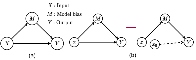
Figure 3: (a) The proposed causal graph. (b) The calculation of total direct effect as in Eq. 7.

3.2.2 Enhancing OIL with Causal Inference

Since the expert is initialized by the source model, when it predicts labels on the test data, its behavior will be affected by the knowledge that it has learned from the source distribution, which is what we call model bias in this work. Since the test distribution is different from the source distribution, and the expert provides instructions to the learner to clone, such model bias will have a negative effect on the learning of the learner. Here, we further use causal inference Pearl (2009) to reduce such effect caused by model bias.

Causal Graph   We assume that the model output of the learner $\pi$ is affected by direct and indirect effect from the input, as shown in the causal graph in Fig. 3a. The causal graph includes the variables which are the input $X$, the output $Y$, and the potential model bias $M$ from the expert. $X\rightarrow Y$ is the direct effect. $X\rightarrow M\rightarrow Y$ represents the indirect effect, where $M$ is a mediator between $X$ and $Y$. $M$ is determined by the input $X$, which can come from in-distribution or out-of-distribution data.

Causal Effects   Our goal in causal inference is to keep the direct effect but control or remove the indirect effect. As shown in Fig. 3b, we calculate the total direct effect (TDE) along $X\rightarrow Y$ as follows:

$$TDE(y) =Y_{y|do(X=x)}-Y_{y|do(X=x_{0})}$$

$$=Y_{y|X=x}-Y_{y|X=x_{0}}$$ (7)

where $do$ operation is the causal intervention Glymour et al. (2016) which is to remove the confounders to $X$. However, since there is no confounder to $X$ in our assumption, we just omit it.

Model Training   Given the total direct effect in Eq. 7, we first have to learn the left term $Y_{y|X=x}$ which is the combination of the direct and indirect effect along $X\rightarrow Y$ and $X\rightarrow M\rightarrow Y$ respectively. We use the learner $\pi$ to learn the direct effect. For the indirect effect, the model bias of $M$ exhibits different behaviors to data from different distributions. Since the learner $\pi$ and the expert $\pi_{e}$ capture the test and source distribution respectively, we use the discrepancy in their outputs to represent the model bias. Considering the model bias, the loss function $l_{t}$ in Eq. 6 becomes:

$$l_{t}(\pi_{t})=\mathbb{I}\big{(}H(p_{t},\hat{y}_{t})<\gamma\big{)}\cdot H\big{(}p_{t}+(p_{t}-\hat{p}_{t}),\hat{y}_{t}\big{)}$$ (8)

where $p_{t}$ and $\hat{p}_{t}$ are the predicted probabilities over the output classes of the learner $\pi_{t}$ and the expert $\pi_{e}$ respectively. $p_{t}$ captures the direct effect and $p_{t}-\hat{p}_{t}$ learns the indirect effect.

Inference   When performing inference, we take the action $y$ which has the largest TDE value. Based on Eq. 7 for TDE calculation, we obtain the prediction over the input $x_{t}$ using the learner $\pi_{t}$ as:

$$y_{t}={\arg\max}_{{i}}TDE({i})=\ \ \ \ \ \ \ \ \ \ \ \ \ \ \ \ \ \ \ \ \ \$$

$$\ \ \ \ \ p_{t}[i]+(1-\beta)\cdot(p_{t}-\hat{p}_{t})[i]$$ (9)

where $\beta$ controls the contribution of the indirect effect. Here, when calculating the TDE score, we assume the model output is zero when given the null input $x_{0}$, since we assume the model cannot make predictions without the given input. We set $\beta$ to 1 throughout the experiments, which completely eliminates the effect of model bias.

0:  Source model $\pi_{0}$; memory bank size $K$; $\alpha$ for expert updating; $\gamma$ for filtering noisy actions; $\beta$ for controlling indirect effect.

1:  Initialize the expert $\pi_{e}\leftarrow\pi_{0}$;

2:  for $t=1,2,\cdots$ do

3:     Return predictions on $x_{t}$ using Eq. 9;

4:     Enqueue ${x}_{t}$ & dequeue ${x}_{t-K}$;

5:     for $x_{k}\in\{x_{t-K},\cdots,x_{t}\}$ do

6:        Use $x_{k}$ to update the learner $\pi_{t}$ as in Eq. 8;

7:        Update the expert $\pi_{e}$ as in Eq. 5;

8:     end for

9:  end for

Algorithm 1 Online Imitation Learning

3.3 Implementation of TTA for the QA Task

For extractive question answering, the model needs to predict the start and end position. The above TTA methods treat the two positions independently and apply the same loss, i.e., $l_{t}(\pi_{t})$, to them separately, and the final loss takes the average of the two. We present the pseudocode of OIL in Algorithm 1, where Tent and PL follow the same procedure but with different losses to update. The data $x_{t}$ at each time $t$ is a batch of instances. We preserve a memory bank with size $K$ to store the data from time $t-K$ to $t$, which more fully exploits test-time data for model adaptation. At each time $t$, we enqueue $x_{t}$ and dequeue $x_{t-K}$ from the memory bank. Then each batch of data from the memory bank is used to optimize the online loss as shown in Eq. 8. The expert for OIL is updated accordingly.

4 Robustness Tuning

In contrast to improving the model post-deployment with TTA, robustness tuning (RT) enhances the model pre-deployment. RT has been studied in NLP to improve model generalization Wang et al. (2022). RT methods are applied at training time when training the source model. We also benchmark RT methods on ColdQA to compare with TTA methods.

First, we compare with adversarial training methods, which are FGM Miyato et al. (2017), PGD Madry et al. (2018), FreeLB Zhu et al. (2020), and InfoBERT Wang et al. (2021a). Next, we further evaluate robustness tuning methods proposed for cross-lingual transfer, which are MVR Wang et al. (2021c) and xTune Zheng et al. (2021). These two methods use regularization to enhance model robustness. All of these methods have not been comprehensively evaluated on distribution shifts arising from text corruption, language change, and domain change.

Combination of RT and TTA.   Finally, we also study combining RT and TTA methods. The source model is tuned by a RT method, then this model is adapted by a TTA method to the test distribution.

Source	$|$Train$|$	$|$Dev$|$	Distribution Shift	Target	$|$Subset$|$	$|$Test$|$	Metric
SQuAD	87,599	34,726	Text corruption	NoiseQA-syn	3	1,190	EM / F1
				NoiseQA-na	3	1,190
			Language change	XQuAD	11	1,190
				MLQA	7	4,517–11,590
			Domain change	HotpotQA	1	5,901
				NaturalQA	1	12,836
				NewsQA	1	4,212
				SearchQA	1	16,980
				TriviaQA	1	7,785

Table 2: Detailed characteristics of ColdQA. To perform evaluation on ColdQA, a model is first trained on the source distribution. Next, the trained model is tested on each subset of each target dataset.

		ColdQA		Text Corruption				Language Change				Domain Change
		Average		NoiseQA-syn		NoiseQA-na		XQuAD		MLQA		MRQA
	Metric	EM	F1	EM	F1	EM	F1	EM	F1	EM	F1	EM	F1
	xlmr-base	55.11	69.21	66.64	78.67	66.05	77.91	55.59	71.42	47.14	65.27	40.11	52.78
RT	MVR	56.93	70.51	68.85	80.10	67.87	78.91	58.08	73.34	48.45	66.33	41.40	53.84
	xTune	58.54	71.94	70.95	81.52	69.75	80.66	58.78	73.75	49.87	67.76	43.36	56.03
TTA	Tent	56.24	69.68	68.02	79.37	67.79	78.91	57.40	72.56	47.59	65.13	40.39	52.43
	PL	56.45	69.78	68.51	79.59	68.15	79.23	57.91	72.69	47.75	65.17	39.94	52.20
	OIL	57.06	70.38	68.75	79.86	68.40	79.40	57.96	72.64	48.39	66.08	41.80	53.92
RT+TTA	xTune + PL	58.86	71.89	71.73	82.12	70.87	81.10	60.23	74.56	50.33	68.10	41.14	53.58
	xTune + OIL	59.63	72.68	71.90	82.24	70.81	81.15	60.13	74.46	50.67	68.53	44.65	57.00
	xlmr-large	58.58	73.82	65.55	79.91	64.17	78.37	63.15	78.77	53.87	72.58	46.18	59.46
RT	FGM	58.06	73.56	64.93	79.71	62.94	77.96	63.21	78.74	54.14	72.72	45.09	58.65
	PGD	58.80	74.02	65.91	80.16	63.75	78.05	63.80	78.91	54.28	72.82	46.25	60.19
	FreeLB	58.79	73.83	66.22	79.97	64.37	77.88	63.34	78.79	53.93	72.51	46.07	59.99
	InfoBERT	57.72	73.39	64.59	79.52	62.66	77.46	62.31	78.28	53.98	72.52	45.05	59.14
	MVR	59.52	74.51	67.06	80.96	64.76	78.59	63.35	78.61	54.47	72.80	47.97	61.60
	xTune	61.51	76.06	70.11	83.17	67.20	80.54	65.00	79.91	56.30	74.33	48.94	62.37
TTA	Tent	54.56	70.34	52.91	69.01	54.29	69.87	63.22	78.91	52.72	70.96	49.65	62.95
	PL	61.80	76.05	71.26	83.60	69.32	81.67	64.05	79.21	54.27	72.57	50.12	63.21
	OIL	62.04	76.19	71.57	83.93	70.11	82.22	64.19	79.37	54.41	72.90	49.93	62.53
RT+TTA	xTune + PL	63.73	77.01	76.01	86.60	73.83	84.55	65.74	80.15	55.78	73.92	47.29	59.81
	xTune + OIL	64.57	77.93	76.13	86.72	73.69	84.61	65.83	80.12	56.24	74.34	51.00	63.86

Table 3: Benchmarking results (%) on ColdQA for XLMR-base and XLMR-large. Each TTA method is run three times with random seeds and the average results are reported. Bold: the best results.

MRQA	HotpotQA	NaturalQA	NewsQA	TriviaQA	SearchQA	Average
xlmr-large	53.13 / 68.19	44.38 / 61.26	45.56 / 63.35	58.25 / 67.16	29.56 / 37.34	46.18 / 59.46
xTune	55.41 / 70.85	47.44 / 63.39	47.98 / 65.58	60.95 / 70.19	32.92 / 41.82	48.94 / 62.37
Tent	53.95 / 69.20	48.14 / 64.34	45.61 / 63.36	58.95 / 67.77	41.61 / 50.09	49.65 / 62.95
PL	53.83 / 69.03	50.88 / 66.17	46.05 / 63.68	58.56 / 67.31	41.26 / 49.84	50.12 / 63.21
OIL	56.65 / 71.92	54.49 / 68.16	46.77 / 64.12	59.18 / 67.99	32.54 / 40.45	49.93 / 62.53
xTune+PL	55.95 / 71.30	53.90 / 68.11	48.50 / 65.72	59.75 / 68.78	18.33 / 25.13	47.29 / 59.81
xTune+OIL	58.46 / 73.99	54.27 / 68.06	47.45 / 64.80	61.05 / 70.21	33.74 / 42.23	51.00 / 63.86

Table 4: Results (EM / F1) on each subset of MRQA. Bold: the best results. Underlined: the second best results.

5 ColdQA

To study robust QA under distribution shifts, in this work we introduce ColdQA, a unified evaluation benchmark against text corruption, language change, and domain change. As shown in Table 2, we collect some existing QA datasets to construct the source and target distributions for ColdQA.

Source Distribution   The training data for the source distribution is SQuAD v1.1 Rajpurkar et al. (2016). To evaluate model generalization on ColdQA, we first need to train a source model with the source training data. Next, we evaluate the model on each subset of each target dataset. For test-time adaptation, the model needs to be adapted with the test data on the fly. To evaluate performance under all kinds of distribution shifts, we use a multilingual pre-trained language model as the base model since it maps different languages into a shared representation space.

Target Distributions    We study the following target distribution shifts at test time.

$\bullet$ Text Corruption  We use NoiseQA to evaluate model robustness to text corruption. NoiseQA Ravichander et al. (2021) studies noises from real-world interfaces, i.e., speech recognizers, keyboards, and translation systems. When humans use these interfaces, the questions asked may contain noises, which degrade the QA system’s performance. NoiseQA includes two subsets, NoiseQA-na and NoiseQA-syn. NoiseQA-na has real-world noises annotated by human annotators, while NoiseQA-syn is synthetically generated.

$\bullet$ Language Change  A robust QA system should also perform well when the inputs are in other languages. We use the datasets XQuAD Artetxe et al. (2020) and MLQA Lewis et al. (2020), designed for cross-lingual transfer, to evaluate change of language in the test data.

$\bullet$ Domain Change  The test data may come from a domain different from the source domain used for model training. Here, the training and test domains are in the same language without any text corruption. We use the datasets from MRQA Fisch et al. (2019) for evaluation, which include HotpotQA Yang et al. (2018), NaturalQA Kwiatkowski et al. (2019), NewsQA Trischler et al. (2017), SearchQA Dunn et al. (2017), and TriviaQA Joshi et al. (2017). The development sets of these datasets are used.

Comparison to Existing Benchmarks   To the best of our knowledge, ColdQA is the first benchmark that unifies robustness evaluation over text corruption, language change, and domain change. Previous benchmarks for robust QA usually only study one type of these distribution shifts, e.g., NoiseQA Ravichander et al. (2021), XTREME Hu et al. (2020), and MRQA Fisch et al. (2019) study text corruption, language change, and domain change respectively, where the methods proposed on these benchmarks are tested only on one type of distribution shifts. So it is unclear if prior proposed methods generalize well to other types of distribution shifts. In contrast, ColdQA evaluates a method on all types of distribution shifts mentioned above, a more challenging task to tackle.

6 Experiments

6.1 Setup

To carry out comprehensive evaluation on all types of distribution shifts, we use a multilingual pre-trained language model as the base model, specifically XLMR-base and XLMR-large Conneau et al. (2020). To train the source model on SQuAD with vanilla fine-tuning, we use the default training setup from Hu et al. (2020). For robustness tuning, we use the hyper-parameter values suggested by Wang et al. (2021a) to train FreeLB and InfoBERT. For MVR and xTune, the default settings from the original work are used.

For test-time adaptation, the details of setting the hyper-parameter values for learning rate, batch size, $\alpha$, $\gamma$, and $K$ are given in Appendix A and shown in Table  10. All model parameters are updated during adaptation. Dropout is turned off for Tent and PL when generating the model outputs or pseudo-labels. The adaptation time of OIL on each dataset from ColdQA is shown in Table 8, 8, and 8. All experiments were performed on one NVIDIA A100 GPU.

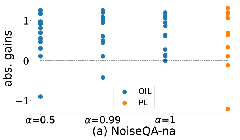
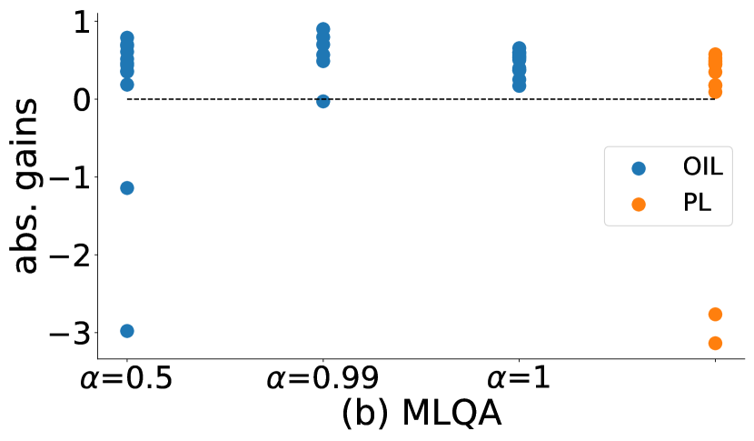
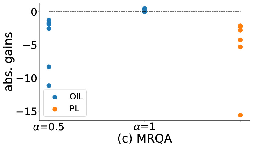
Figure 4: Robustness of PL and OIL to variance of hyper-parameter values. With OIL and PL, we adapt XLMR-base tuned by xTune by using various value combinations of hyper-parameters, which are learning rate and memory size. Learning rate is selected from {5e-6, 1e-6, 5e-7, 1e-7} and memory size from {1, 3, 5}. For OIL, different values of $\alpha$ are tested.

6.2 Main Results

Table 3 shows the benchmarking results of TTA, RT, and their combination on ColdQA. The detailed results on each subset of MRQA are reported in Table 4. We have the following observations.

ColdQA is challenging on which not all RT methods are effective.   In Fig. 7 from the appendix, we report the gains of RT baselines over vanilla fine-tuning on the development set of SQuAD. Not surprisingly, each RT baseline improves the model results on the in-distribution set. However, after re-benchmarking the RT baselines on ColdQA, we see that xTune and MVR are more effective than the adversarial training baselines. Among the adversarial training methods, only PGD and FreeLB can improve the average results but the improvements are marginal. Overall, ColdQA introduces new challenges to the existing RT methods.

OIL is stronger than PL and Tent.   Tent is much less effective than OIL and PL on ColdQA though it is a very strong baseline on CV tasks Wang et al. (2021b). This shows the necessity of re-analyzing TTA methods on QA tasks. OIL is consistently better than PL based on the average results in Table 3. OIL mostly outperforms Tent and PL based on the detailed results of MRQA in Table 4.

TTA and RT are both effective and they are comparable to each other.   On XLMR-base and XLMR-large, both TTA (OIL and PL) and RT (xTune and MVR) can significantly improve the average results by around 1-3 absolute points. Overall, TTA and RT are comparable to each other. More specifically, on XLMR-large, the best TTA method which is OIL outperforms xTune on the average results. On XLMR-large, OIL is better than xTune on NoiseQA and MRQA, but lags behind xTune on XQuAD and MLQA. However, on XLMR-base, TTA does not outperform RT. We think the reason is that the effectiveness of TTA depends on the source model, since TTA starts from the source model and the source model decides the accuracy of predicted pseudo-labels on the test data.

Applying TTA after RT significantly boosts the performance and achieves SOTA results. On both XLMR-base and XLMR-large, xTune+OIL achieves the best average performance compared to all other methods. On XLMR-large, xTune+OIL improves xTune by 3 points on EM score. Among the three types of distribution shifts, xTune+OIL is more effective on text corruption and domain change than language change. Finally, xTune+OIL improves over the baseline EM score by more than 4 points on XLMR-base and 6 points on XLMR-large, significantly improving QA robustness against distribution shifts.

EM / F1	Avg.	NoiseQA-syn	NoiseQA-na	XQuAD	MLQA	MRQA
OIL	57.06 / 70.38	68.75 / 79.86	68.40 / 79.40	57.96 / 72.64	48.39 / 66.08	41.80 / 53.92
w/o CI	56.68 / 69.85	68.41 / 79.48	68.11 / 79.14	57.98 / 72.43	48.08 / 65.65	40.82 / 52.57
xTune + OIL	59.63 / 72.68	71.90 / 82.24	70.81 / 81.15	60.13 / 74.46	50.67 / 68.53	44.65 / 57.00
w/o CI	59.06 / 72.11	71.13 / 81.76	70.18 / 80.64	59.73 / 73.93	50.49 / 68.31	43.75 / 55.92

Table 5: Effects of causal inference on XLMR-base. CI: causal inference

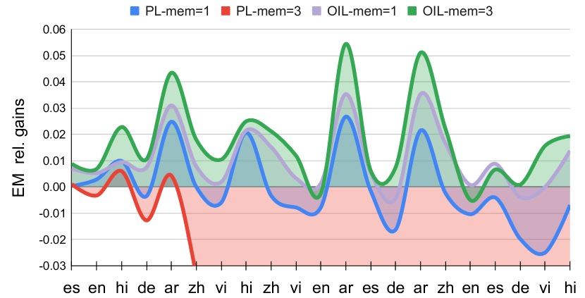
Figure 5: Robustness of PL and OIL to changes of test distribution over time. $y$-axis shows relative gains on each language over XLMR-base tuned by xTune. $x$-axis shows test sets from MLQA. mem: memory size $K$. OIL sets $\alpha$ to 0.999.

6.3 Further Analysis

Compared to PL, OIL is more robust to varying hyper-parameter values.   OIL utilizes an expert model to perform model adaptation. $\alpha$ controls updating of the expert model. In Fig. 4, we fix the value of $\alpha$, adapt the model with various combinations of hyper-parameter values, and report the absolute gains on EM score after adaptation. We observe that for OIL, a higher $\alpha$ value such as 0.99 or 1 achieves positive gains under varying hyper-parameter values. However, PL is less stable than OIL under varying hyper-parameter values. To be robust to varying hyper-parameter values is important for TTA, since tuning hyper-parameters on unknown test data is difficult.

OIL is better than PL when dealing with changes in test distribution.   We further evaluate TTA methods in the setting of continual adaptation, where the test distribution changes over time (rather than staying fixed as in Table 3), and the model needs to be adapted continually without stopping. In Fig. 5, we adapt the source model from the test language of es to the language hi without stopping. On each test distribution, we report the relative gain over the source model without adaptation. We find that PL is less robust in such a setting and often has negative gains, especially in the last few adaptations. However, our proposed method OIL achieves positive gains among nearly all adaptations, which demonstrates the robustness of OIL in continual adaptation.

Effects of Causal Inference.   Table 5 shows the effects of removing causal inference in OIL. Without causal inference, adaptation performance consistently drops on the test sets. In Fig. 6, we further show how $\beta$ affects causal inference. $\beta$ does affect the final results and the optimal $\beta$ value varies with different datasets. To avoid tuning $\beta$, model bias is completely removed by setting $\beta$ to 1 in all our experiments.

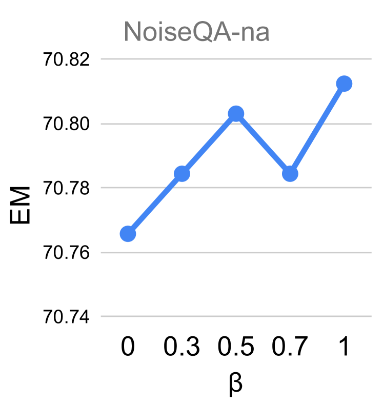
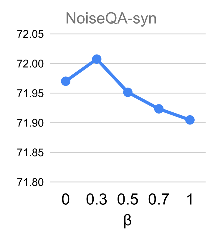
Figure 6: The effects of $\beta$ used in causal inference. Results are evaluated on NoiseQA with XLMR-base tuned by xTune.

7 Conclusion

We study test-time adaptation (TTA) for robust question answering under distribution shifts. A unified evaluation benchmark, ColdQA, over text corruption, language change, and domain change is provided. A novel TTA method, OIL, is proposed that achieves good performance when combined with a robustness tuning method.

Limitations

Though test-time adaptation shows strong improvements for robust QA under distribution shifts, it still has some issues that need to be addressed in the future. First, model updating is costly. TTA needs to update the model online. However, the cost of updating should be controlled especially for large pre-trained language models. Second, how to choose suitable hyper-parameter values for adaptation is also important. The test data is usually not available and we cannot tune the hyper-parameters before adaptation, so how to effectively select hyper-parameter values is important. In our work, we did not perform hyper-parameter search for OIL. We have also demonstrated in Fig 4 that OIL is robust to various combinations of hyper-parameter values with the help of the expert model.

Appendix A Appendix

OIL	HotpotQA	NaturalQA	NewsQA	SearchQA	TriviaQA
xlmr-base	247	771	502	1265	579
xlmr-large	1116	3450	1441	6779	4369

Table 6: Adaptation time (in seconds) on MRQA.

	MLQA
OIL	en	es	de	ar	hi	vi	zh
xlmr-base	489	159	164	218	203	239	172
xlmr-large	1635	533	548	724	679	802	574

Table 7: Adaptation time (in seconds) on MLQA.

OIL	XQuAD	NoiseQA
xlmr-base	124	162
xlmr-large	187	193

Table 8: Adaptation time (in seconds) on each subset of XQuAD and NoiseQA.

NoiseQA-na	OIL		w/o denoise
XLMR-base	EM	F1	EM	F1
asr	63.59	74.74	62.35	74.05
keyboard	72.04	82.90	72.18	83.21
translation	69.58	80.55	70.08	81.18
avg.	68.40	79.40	68.21	79.48
XLMR-large	EM	F1	EM	F1
asr	62.10	75.34	47.98	66.36
keyboard	74.96	86.61	74.43	86.24
translation	73.28	84.72	73.14	84.70
avg.	70.11	82.22	65.18	79.10
NoiseQA-syn	OIL		w/o denoise
XLMR-base	EM	F1	EM	F1
asr	70.14	81.97	69.55	81.59
keyboard	66.97	77.29	66.72	77.41
translation	69.13	80.31	69.16	80.19
avg.	68.75	79.86	68.48	79.73
XQuAD	OIL		w/o denoise
XLMR-base	EM	F1	EM	F1
en	72.83	83.75	72.91	83.89
es	60.14	77.37	59.55	77.33
de	58.18	74.25	58.63	74.48
el	56.58	73.05	56.13	73.15
ru	58.26	74.28	58.18	74.51
tr	52.38	67.89	51.57	68.01
ar	49.89	66.40	49.83	66.72
vi	54.99	73.83	55.41	74.11
th	63.59	72.22	62.21	71.58
zh	59.66	68.59	58.15	67.85
hi	51.04	67.38	51.09	68.17
avg.	57.96	72.64	57.61	72.71

Table 9: Effects of not filtering noisy labels in OIL for NoiseQA and XQuAD.

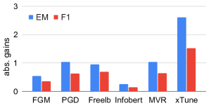
Figure 7: Gains over the results of XLMR-large with vanilla fine-tuning on the development set of SQuAD. abs.: absolute.

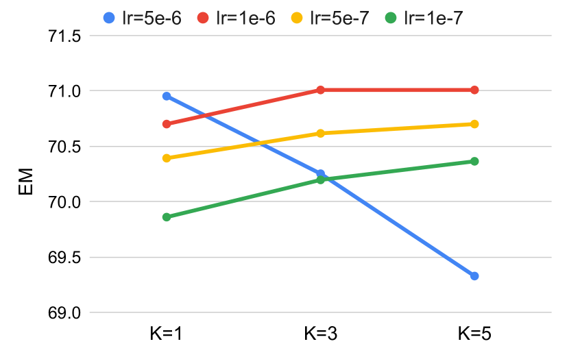
Figure 8: Effects of memory size $K$ on NoiseQA-na. The source model is XLMR-base tuned by xTune.

Dataset	NoiseQA	XQuAD	MLQA	HotpotQA	NaturalQA	NewsQA	SearchQA	TriviaQA
|Size|	1,190	1,190	4,517–11,590	5,901	12,836	4,212	16,980	7,785
OIL	$K$: 5 $\gamma$: 0.5 $\alpha$: 0.99 $\beta$: 1 BATCH_SIZE: 8 LR: 1e-6	$K$: 5 $\gamma$: 0.5 $\alpha$: 0.99 $\beta$: 1 BATCH_SIZE: 8 LR: 1e-6	$K$: 3 $\gamma$: $\infty$ $\alpha$: 0.99 $\beta$: 1 BATCH_SIZE: 16 LR: 1e-6	$K$: 3 $\gamma$: $\infty$ $\alpha$: 0.99 $\beta$: 1 BATCH_SIZE: 16 LR: 1e-6	$K$: 3 $\gamma$: 0.5 $\alpha$: 0.99 $\beta$:1 BATCH_SIZE: 16 LR: 1e-6	$K$: 3 $\gamma$: $\infty$ $\alpha$: 0.99 $\beta$: 1 BATCH_SIZE: 16 LR: 1e-6	$K$: 1 $\gamma$: $\infty$ $\alpha$: 1 $\beta$:1 BATCH_SIZE: 16 LR: 1e-6	$K$: 1 $\gamma$: $\infty$ $\alpha$: 1 $\beta$: 1 BATCH_SIZE: 16 LR: 1e-6
PL	$K$: 5 BATCH_SIZE: 8 LR: 1e-6	$K$: 5 BATCH_SIZE: 8 LR: 1e-6	$K$: 3 BATCH_SIZE: 16 LR: 1e-6	$K$: 1 BATCH_SIZE: 16 LR: 1e-7	$K$: 1 BATCH_SIZE: 16 LR: 1e-7	$K$: 1 BATCH_SIZE: 16 LR: 1e-7	$K$: 1 BATCH_SIZE: 16 LR: 1e-7	$K$: 1 BATCH_SIZE: 16 LR: 1e-7
Tent	$K$: 5 BATCH_SIZE: 8 LR: 1e-6	$K$: 5 BATCH_SIZE: 8 LR: 1e-6	$K$: 3 BATCH_SIZE: 16 LR: 1e-6	$K$: 1 BATCH_SIZE: 16 LR: 1e-7	$K$: 1 BATCH_SIZE: 16 LR: 1e-7	$K$: 1 BATCH_SIZE: 16 LR: 1e-7	$K$: 1 BATCH_SIZE: 16 LR: 1e-7	$K$: 1 BATCH_SIZE: 16 LR: 1e-7

Table 10: Hyper-parameters for TTA baselines. For MRQA, we find that for PL and OIL, when we keep the same learning rate and batch size as OIL, the final results are bad, so we choose better hyper-parameters for PL and Tent as the table shows.

A.1 Hyper-parameters

We provide the values of hyper-parameters for test-time adaptation. (1) For learning rate, we select a value smaller than the one used for training the source model. We set the learning rate to 1e-6. (2) For batch size, for smaller test sets, we set the batch size to 8. For larger test sets, we set the batch size to 16. (3) For $\alpha$ used in updating the expert model, if the test set is large, we set $\alpha$ to a larger value such as 1. Otherwise, we set $\alpha$ to a smaller value such as 0.99. (4) For $\gamma$ used in filtering the noisy labels, $\gamma=\infty$ works well for most of the test sets, except the datasets NoiseQA, XQuAD, and NaturalQA, where we set $\gamma$ to 0.5. (5) For memory size $K$, we set $K$ to a smaller value for large sets but to a larger value for small sets. The specific hyper-parameters used for TTA baselines are presented in Table 10.

Appendix B Effects of Denoising in OIL

Table 9 shows the effects of denoising in OIL. For NoiseQA and XQuAD, we set $\gamma$ to 0.5 to filter out the noisy labels. When using XLMR-large as the base model for NoiseQA-na, the average performance drops substantially if noisy labels are not removed.

Appendix C Results of RT methods on the Development Set of SQuAD

Fig. 7 shows the gains on the development set of SQuAD trained by each RT baseline, to demonstrate the effectiveness of the RT methods.

Appendix D Effects of Memory Size $K$

Fig. 8 shows the effects of memory size $K$. We see that using a larger memory size can improve the adaptation results when the learning rate is not so large. When the learning rate is large, larger memory size can worsen the results.

References

- Artetxe et al. (2020) Mikel Artetxe, Sebastian Ruder, and Dani Yogatama. 2020. On the cross-lingual transferability of monolingual representations. In Proceedings of the Annual Meeting of the Association for Computational Linguistics.
- Banerjee et al. (2021) Pratyay Banerjee, Tejas Gokhale, and Chitta Baral. 2021. Self-supervised test-time learning for reading comprehension. In Proceedings of the Conference of the North American Chapter of the Association for Computational Linguistics: Human Language Technologies.
- Bartler et al. (2022) Alexander Bartler, Andre Bühler, Felix Wiewel, Mario Döbler, and Bin Yang. 2022. MT3: Meta test-time training for self-supervised test-time adaption. In Proceedings of the International Conference on Artificial Intelligence and Statistics.
- Belinkov and Bisk (2018) Yonatan Belinkov and Yonatan Bisk. 2018. Synthetic and natural noise both break neural machine translation. In International Conference on Learning Representations.
- Ben-David et al. (2022) Eyal Ben-David, Nadav Oved, and Roi Reichart. 2022. PADA: Example-based prompt learning for on-the-fly adaptation to unseen domains. Transactions of the Association for Computational Linguistics.
- Ben-David et al. (2010) Shai Ben-David, John Blitzer, Koby Crammer, Alex Kulesza, Fernando Pereira, and Jennifer Wortman Vaughan. 2010. A theory of learning from different domains. Machine Learning.
- Cheng et al. (2021) Hao Cheng, Xiaodong Liu, Lis Pereira, Yaoliang Yu, and Jianfeng Gao. 2021. Posterior differential regularization with f-divergence for improving model robustness. In Proceedings of the Conference of the North American Chapter of the Association for Computational Linguistics: Human Language Technologies.
- Conneau et al. (2020) Alexis Conneau, Kartikay Khandelwal, Naman Goyal, Vishrav Chaudhary, Guillaume Wenzek, Francisco Guzmán, Edouard Grave, Myle Ott, Luke Zettlemoyer, and Veselin Stoyanov. 2020. Unsupervised cross-lingual representation learning at scale. In Proceedings of the Annual Meeting of the Association for Computational Linguistics.
- Dunn et al. (2017) Matthew Dunn, Levent Sagun, Mike Higgins, V. Ugur Güney, Volkan Cirik, and Kyunghyun Cho. 2017. SearchQA: A new Q&A dataset augmented with context from a search engine. ArXiv preprint, abs/1704.05179.
- Fisch et al. (2019) Adam Fisch, Alon Talmor, Robin Jia, Minjoon Seo, Eunsol Choi, and Danqi Chen. 2019. MRQA 2019 shared task: Evaluating generalization in reading comprehension. In Proceedings of the 2nd Workshop on Machine Reading for Question Answering.
- Gan and Ng (2019) Wee Chung Gan and Hwee Tou Ng. 2019. Improving the robustness of question answering systems to question paraphrasing. In Proceedings of the Annual Meeting of the Association for Computational Linguistics.
- Gao et al. (2022) Ge Gao, Eunsol Choi, and Yoav Artzi. 2022. Simulating bandit learning from user feedback for extractive question answering. In Proceedings of the Annual Meeting of the Association for Computational Linguistics (Volume 1: Long Papers).
- Glymour et al. (2016) Madelyn Glymour, Judea Pearl, and Nicholas P Jewell. 2016. Causal Inference in Statistics: A Primer. John Wiley & Sons.
- He et al. (2021) Ruidan He, Linlin Liu, Hai Ye, Qingyu Tan, Bosheng Ding, Liying Cheng, Jiawei Low, Lidong Bing, and Luo Si. 2021. On the effectiveness of adapter-based tuning for pretrained language model adaptation. In Proceedings of the Annual Meeting of the Association for Computational Linguistics and the International Joint Conference on Natural Language Processing (Volume 1: Long Papers).
- Hu et al. (2020) Junjie Hu, Sebastian Ruder, Aditya Siddhant, Graham Neubig, Orhan Firat, and Melvin Johnson. 2020. XTREME: A massively multilingual multi-task benchmark for evaluating cross-lingual generalisation. In Proceedings of the International Conference on Machine Learning.
- Jia and Liang (2017) Robin Jia and Percy Liang. 2017. Adversarial examples for evaluating reading comprehension systems. In Proceedings of the Conference on Empirical Methods in Natural Language Processing.
- Jiang et al. (2020) Haoming Jiang, Pengcheng He, Weizhu Chen, Xiaodong Liu, Jianfeng Gao, and Tuo Zhao. 2020. SMART: Robust and efficient fine-tuning for pre-trained natural language models through principled regularized optimization. In Proceedings of the Annual Meeting of the Association for Computational Linguistics.
- Joshi et al. (2017) Mandar Joshi, Eunsol Choi, Daniel Weld, and Luke Zettlemoyer. 2017. TriviaQA: A large scale distantly supervised challenge dataset for reading comprehension. In Proceedings of the Annual Meeting of the Association for Computational Linguistics (Volume 1: Long Papers).
- Karouzos et al. (2021) Constantinos Karouzos, Georgios Paraskevopoulos, and Alexandros Potamianos. 2021. UDALM: Unsupervised domain adaptation through language modeling. In Proceedings of the Conference of the North American Chapter of the Association for Computational Linguistics: Human Language Technologies.
- Kwiatkowski et al. (2019) Tom Kwiatkowski, Jennimaria Palomaki, Olivia Redfield, Michael Collins, Ankur Parikh, Chris Alberti, Danielle Epstein, Illia Polosukhin, Jacob Devlin, Kenton Lee, Kristina Toutanova, Llion Jones, Matthew Kelcey, Ming-Wei Chang, Andrew M. Dai, Jakob Uszkoreit, Quoc Le, and Slav Petrov. 2019. Natural Questions: A benchmark for question answering research. Transactions of the Association for Computational Linguistics.
- Lee (2013) Dong-Hyun Lee. 2013. Pseudo-Label: the simple and efficient semi-supervised learning method for deep neural networks. In ICML Workshop on Challenges in Representation Learning.
- Lester et al. (2021) Brian Lester, Rami Al-Rfou, and Noah Constant. 2021. The power of scale for parameter-efficient prompt tuning. In Proceedings of the Conference on Empirical Methods in Natural Language Processing.
- Lewis et al. (2020) Patrick Lewis, Barlas Oguz, Ruty Rinott, Sebastian Riedel, and Holger Schwenk. 2020. MLQA: Evaluating cross-lingual extractive question answering. In Proceedings of the Annual Meeting of the Association for Computational Linguistics.
- Li et al. (2020) Juntao Li, Ruidan He, Hai Ye, Hwee Tou Ng, Lidong Bing, and Rui Yan. 2020. Unsupervised domain adaptation of a pretrained cross-lingual language model. In Proceedings of the Twenty-Ninth International Joint Conference on Artificial Intelligence.
- Li et al. (2022) Zichao Li, Prakhar Sharma, Xing Han Lu, Jackie Chi Kit Cheung, and Siva Reddy. 2022. Using interactive feedback to improve the accuracy and explainability of question answering systems post-deployment. In Findings of the Association for Computational Linguistics.
- Liang et al. (2020) Jian Liang, Dapeng Hu, and Jiashi Feng. 2020. Do we really need to access the source data? source hypothesis transfer for unsupervised domain adaptation. In Proceedings of the International Conference on Machine Learning.
- Lin et al. (2022) Bill Yuchen Lin, Sida Wang, Xi Lin, Robin Jia, Lin Xiao, Xiang Ren, and Scott Yih. 2022. On continual model refinement in out-of-distribution data streams. In Proceedings of the Annual Meeting of the Association for Computational Linguistics (Volume 1: Long Papers).
- Liu et al. (2021a) Jiexi Liu, Ryuichi Takanobu, Jiaxin Wen, Dazhen Wan, Hongguang Li, Weiran Nie, Cheng Li, Wei Peng, and Minlie Huang. 2021a. Robustness testing of language understanding in task-oriented dialog. In Proceedings of the Annual Meeting of the Association for Computational Linguistics and the International Joint Conference on Natural Language Processing (Volume 1: Long Papers).
- Liu et al. (2021b) Yuejiang Liu, Parth Kothari, Bastien van Delft, Baptiste Bellot-Gurlet, Taylor Mordan, and Alexandre Alahi. 2021b. TTT++: When does self-supervised test-time training fail or thrive? In Advances in Neural Information Processing Systems: Annual Conference on Neural Information Processing Systems.
- Madry et al. (2018) Aleksander Madry, Aleksandar Makelov, Ludwig Schmidt, Dimitris Tsipras, and Adrian Vladu. 2018. Towards deep learning models resistant to adversarial attacks. In International Conference on Learning Representations.
- Miyato et al. (2017) Takeru Miyato, Andrew M. Dai, and Ian J. Goodfellow. 2017. Adversarial training methods for semi-supervised text classification. In International Conference on Learning Representations.
- Parisi et al. (2019) German I Parisi, Ronald Kemker, Jose L Part, Christopher Kanan, and Stefan Wermter. 2019. Continual lifelong learning with neural networks: A review. Neural Networks, 113.
- Pearl (2009) Judea Pearl. 2009. Causal inference in statistics: An overview. Statistics Surveys, 3.
- Peng et al. (2021) Baolin Peng, Chunyuan Li, Zhu Zhang, Chenguang Zhu, Jinchao Li, and Jianfeng Gao. 2021. RADDLE: An evaluation benchmark and analysis platform for robust task-oriented dialog systems. In Proceedings of the Annual Meeting of the Association for Computational Linguistics and the International Joint Conference on Natural Language Processing (Volume 1: Long Papers).
- Rajpurkar et al. (2016) Pranav Rajpurkar, Jian Zhang, Konstantin Lopyrev, and Percy Liang. 2016. SQuAD: 100,000+ questions for machine comprehension of text. In Proceedings of the Conference on Empirical Methods in Natural Language Processing.
- Ramponi and Plank (2020) Alan Ramponi and Barbara Plank. 2020. Neural unsupervised domain adaptation in NLP—A survey. In Proceedings of the 28th International Conference on Computational Linguistics.
- Ravichander et al. (2021) Abhilasha Ravichander, Siddharth Dalmia, Maria Ryskina, Florian Metze, Eduard Hovy, and Alan W Black. 2021. NoiseQA: Challenge set evaluation for user-centric question answering. In Proceedings of the Conference of the European Chapter of the Association for Computational Linguistics: Main Volume.
- Ribeiro et al. (2020) Marco Tulio Ribeiro, Tongshuang Wu, Carlos Guestrin, and Sameer Singh. 2020. Beyond accuracy: Behavioral testing of NLP models with CheckList. In Proceedings of the Annual Meeting of the Association for Computational Linguistics.
- Ross et al. (2011) Stéphane Ross, Geoffrey Gordon, and Drew Bagnell. 2011. A reduction of imitation learning and structured prediction to no-regret online learning. In Proceedings of the Fourteenth International Conference on Artificial Intelligence and Statistics.
- Rychalska et al. (2019) Barbara Rychalska, Dominika Basaj, Alicja Gosiewska, and Przemysław Biecek. 2019. Models in the wild: On corruption robustness of neural NLP systems. In Proceedings of the International Conference on Neural Information Processing.
- Su et al. (2022) Xin Su, Yiyun Zhao, and Steven Bethard. 2022. A comparison of strategies for source-free domain adaptation. In Proceedings of the Annual Meeting of the Association for Computational Linguistics (Volume 1: Long Papers).
- Sun et al. (2020) Yu Sun, Xiaolong Wang, Zhuang Liu, John Miller, Alexei A. Efros, and Moritz Hardt. 2020. Test-time training with self-supervision for generalization under distribution shifts. In Proceedings of the International Conference on Machine Learning.
- Tarvainen and Valpola (2017) Antti Tarvainen and Harri Valpola. 2017. Mean teachers are better role models: Weight-averaged consistency targets improve semi-supervised deep learning results. In Advances in Neural Information Processing Systems: Annual Conference on Neural Information Processing Systems.
- Trischler et al. (2017) Adam Trischler, Tong Wang, Xingdi Yuan, Justin Harris, Alessandro Sordoni, Philip Bachman, and Kaheer Suleman. 2017. NewsQA: A machine comprehension dataset. In Proceedings of the 2nd Workshop on Representation Learning for NLP.
- Tu et al. (2020) Lifu Tu, Garima Lalwani, Spandana Gella, and He He. 2020. An empirical study on robustness to spurious correlations using pre-trained language models. Transactions of the Association for Computational Linguistics.
- Wang et al. (2021a) Boxin Wang, Shuohang Wang, Yu Cheng, Zhe Gan, Ruoxi Jia, Bo Li, and Jingjing Liu. 2021a. InfoBERT: improving robustness of language models from an information theoretic perspective. In International Conference on Learning Representations.
- Wang et al. (2021b) Dequan Wang, Evan Shelhamer, Shaoteng Liu, Bruno A. Olshausen, and Trevor Darrell. 2021b. Tent: Fully test-time adaptation by entropy minimization. In International Conference on Learning Representations.
- Wang et al. (2021c) Xinyi Wang, Sebastian Ruder, and Graham Neubig. 2021c. Multi-view subword regularization. In Proceedings of the Conference of the North American Chapter of the Association for Computational Linguistics: Human Language Technologies.
- Wang et al. (2021d) Xinyi Wang, Yulia Tsvetkov, Sebastian Ruder, and Graham Neubig. 2021d. Efficient test time adapter ensembling for low-resource language varieties. In Findings of the Association for Computational Linguistics.
- Wang et al. (2022) Xuezhi Wang, Haohan Wang, and Diyi Yang. 2022. Measure and improve robustness in NLP models: A survey. In Proceedings of the 2022 Conference of the North American Chapter of the Association for Computational Linguistics: Human Language Technologies.
- Yang et al. (2018) Zhilin Yang, Peng Qi, Saizheng Zhang, Yoshua Bengio, William Cohen, Ruslan Salakhutdinov, and Christopher D. Manning. 2018. HotpotQA: A dataset for diverse, explainable multi-hop question answering. In Proceedings of the Conference on Empirical Methods in Natural Language Processing.
- Ye et al. (2022) Hai Ye, Hwee Tou Ng, and Wenjuan Han. 2022. On the robustness of question rewriting systems to questions of varying hardness. In Proceedings of the Annual Meeting of the Association for Computational Linguistics (Volume 1: Long Papers).
- Ye et al. (2020) Hai Ye, Qingyu Tan, Ruidan He, Juntao Li, Hwee Tou Ng, and Lidong Bing. 2020. Feature adaptation of pre-trained language models across languages and domains with robust self-training. In Proceedings of the Conference on Empirical Methods in Natural Language Processing.
- Zheng et al. (2021) Bo Zheng, Li Dong, Shaohan Huang, Wenhui Wang, Zewen Chi, Saksham Singhal, Wanxiang Che, Ting Liu, Xia Song, and Furu Wei. 2021. Consistency regularization for cross-lingual fine-tuning. In Proceedings of the Annual Meeting of the Association for Computational Linguistics and the International Joint Conference on Natural Language Processing (Volume 1: Long Papers).
- Zhu et al. (2020) Chen Zhu, Yu Cheng, Zhe Gan, Siqi Sun, Tom Goldstein, and Jingjing Liu. 2020. FreeLB: Enhanced adversarial training for natural language understanding. In International Conference on Learning Representations.