Measurements of two-pion HBT correlations in Be+Be collisions at 150$A\,\mbox{Ge\kern-1.00006ptV}\!/\!c$ beam momentum, at the NA61/SHINE experiment at CERN CERN-EP-2023-013 Eur. Phys. J. C This paper reports measurements of two-pion Bose-Einstein (HBT) correlations in Be+Be collisions at a beam momentum of 150$A\,\mbox{Ge\kern-1.00006ptV}\!/\!c$ by the NA61/SHINE experiment at the CERN SPS accelerator. The obtained momentum space correlation functions can be well described by a Lévy distributed source model. The transverse mass dependence of the Lévy source parameters is presented, and their possible theoretical interpretations are discussed. The results show that the Lévy exponent $\alpha$ is approximately constant as a function of $m_{\textnormal{T}}$, and far from both the Gaussian case of $\alpha=2$ or the conjectured value at the critical endpoint, $\alpha=0.5$. The radius scale parameter $R$ shows a slight decrease in $m_{\textnormal{T}}$, which can be explained as a signature of transverse flow. Finally, an approximately constant trend of the intercept parameter $\lambda$ as a function of $m_{\textnormal{T}}$ was observed, different from measurement results at RHIC.

1 Introduction

This paper reports measurements of quantum-statistical Bose-Einstein correlation functions for identified, like-sign charged pion pairs, produced in central Be+Be collisions at 150A GeV/c beam momentum.

The method of quantum-statistical (Bose-Einstein) correlations was first applied in astrophysical intensity correlation measurements by R. Hanbury Brown and R. Q. Twiss (HBT) [1] in order to determine the apparent angular diameter of stellar objects. Later, a similar quantum-statistical method was applied in momentum correlation measurements for proton-antiproton collisions [2, 3], for obtaining information on the size parameters of particle emission sources in high-energy particle collisions. Since then quantum-statistical (HBT) correlation measurements became a standard tool for experimental characterization of the probability density in particle emission process, i.e. the source function which sheds light on the spatio-temporal structure of particle emission. This experimental method also largely contributed to the understanding of the hydro-dynamical nature of the produced strongly interacting matter. In fact, the pair momentum dependence of Gaussian shaped source radii [4, 5] can be well explained by a hydro-dynamical expansion. The shape of the particle emitting source was furthermore suggested to be affected by the nature of the quark-hadron transition [6]. Hence the exploration of HBT correlations is of utmost importance in the quest for understanding the nature of the matter created in relativistic heavy-ion collisions.

The results presented in this paper were obtained by the NA61/SHINE [7] experiment at the CERN Super Proton Synchrotron accelerator. This measurement is part of the NA61/SHINE strong interaction program investigating the properties of the onset of deconfinement and searching for the possible existence of the critical point of strongly interacting matter. This goal is pursued by the NA61/SHINE collaboration by a beam energy scan with various nucleus-nucleus collisions. This strategy allows to systematically investigate properties of the phase diagram of strongly interacting matter [8].

Within the framework of statistical models the data on particle production suggest that with increasing collision energy, the temperature increases and baryon chemical potential of strongly interacting matter decreases at freeze-out, whereas by increasing the nuclear mass number of the colliding nuclei the temperature decreases [9, 10]. As a result of the NA61/SHINE research program, a large set of collision data on p+p, p+Pb, Be+Be, Ar+Sc, Xe+La and Pb+Pb collision systems has already been recorded. An upgrade of the NA61/SHINE experiment was completed in 2022 and further high-statistics data on Pb+Pb collisions will be collected in the near future [11]. A basic reference has already been established with p+p, Be+Be and Ar+Sc interactions on particle spectra and multiplicities [12, 13, 14, 15, 16, 17]. The present paper provides results on Bose-Einstein correlations of identified, like-sign pion pairs in 0–20% centrality selected ⁷Be+⁹Be collisions. The data were recorded in 2011, 2012 and 2013 using a secondary ⁷Be beam produced by fragmentation of the primary Pb beam from the CERN SPS [18].

In NA61/SHINE collision centrality is characterized via the energy detected in the region populated by projectile spectators. Central collisions are selected by lower values of this very forward energy. Although for smaller systems, such as Be+Be collisions, the very forward energy is not expected to be tightly correlated with the actual impact parameter of the collision, the terms central and centrality are still adopted following the convention widely used in heavy-ion physics.

The paper is organized as follows. Section 2 recalls the fundamental theory behind the technique of Bose-Einstein correlations in order to fix notations. In Section 3, the NA61/SHINE detector is described. In Section 4, the details of the analysis procedure are discussed. In Section 5, the obtained experimental results are presented. The paper closes with Section 6 summarizing the results and conclusions.

2 Bose-Einstein correlations

2.1 Bose-Einstein correlation functions

The two-particle Bose-Einstein correlations are defined in terms of the single- and the two-particle invariant momentum distributions $N_{1}$ and $N_{2}$ as:

$$C_{2}(p_{1},p_{2})=\frac{N_{2}(p_{1},p_{2})}{N_{1}(p_{1})N_{1}(p_{2})},$$ (1)

where $p_{1}$ and $p_{2}$ are the momenta of the individual particles. If the $S(x,p)$ (source function) denotes the probability density of particle creation at space-time point $x$ and momentum $p$, the momentum distribution of emitted particles can be expressed via this source function as [19]:

$$N_{1}(p_{1}) =\int S(x_{1},p_{1})|\Psi_{p}(x_{1})|^{2}d^{4}x_{1},$$ (2)

$$N_{2}(p_{1},p_{2}) =\int S(x_{1},p_{1})S(x_{2},p_{2})|\Psi_{p_{1},p_{2}}(x_{1},x_{2})|^{2}d^{4}x_{2}d^{4}x_{1},$$ (3)

where $\Psi_{p}(x)$ and $\Psi_{p_{1},p_{2}}(x_{1},x_{2})$ are the single- and two-particle wave functions. In the case of the single-particle wave function, $|\Psi_{p}(x)|^{2}=1$ holds, whereas for the two-particle wave function, taking into account the Bose-Einstein symmetrisation, one has [20]:

$$|\Psi_{p_{1},p_{2}}(x_{1},x_{2})|^{2}=1+\cos(qx),$$ (4)

where $x=x_{1}-x_{2}$ is the relative coordinate and $q=p_{1}-p_{2}$ is the relative momentum of the pair. In the $qx$ term a division by $\hbar$ is suppressed, and throughout this paper we will utilize the $\hbar=1$ convention. Substituting the above equation into Eq. (1), one infers

$$C_{2}(p_{1},p_{2})=1+\frac{\tilde{S}(q,p_{1})\tilde{S}(q,p_{2})^{*}}{\tilde{S}(q=0,p_{1})\tilde{S}(q=0,p_{2})^{*}},$$ (5)

where $\tilde{S}$ is the Fourier transform of $S$. If relative momentum $q$ is much smaller compared to the average momentum of the pair $K=(p_{1}+p_{2})/2$, then Eq. (5) can be expressed as:

$$C_{2}(q,K)=1+\frac{|\tilde{S}(q,K)|^{2}}{|\tilde{S}(q=0,K)|^{2}}.$$ (6)

Alternatively, with a simplified notation where the $K$-dependence is suppressed and a normalized source is assumed, one may write $C_{2}(q)=1+|\tilde{S}(q)|^{2}$. This choice is motivated by the so-called smoothness approximation [21]. The dependence on relative momentum $q$ is stronger than on the average momentum of the pair $K$, hence $q$ is considered as the more important variable of the correlation function, and the other variable is mostly suppressed in the notation. When the correlation function is parameterized based on an ansatz for the source function, its parameters can depend on $K$. In order to explore the transverse dynamics of the source, the average transverse momentum of the pair, $K_{T}=\frac{1}{2}\sqrt{K^{2}_{x}+K_{y}^{2}}$ is introduced, as usual. Furthermore, motivated by hydro-dynamical considerations, the dependence on the transverse mass $m_{T}=\sqrt{m^{2}c^{4}+K_{T}^{2}c^{2}}$ is often studied, where $m$ is the particle mass. The $m_{T}$-dependence of the source parameters, such as its width, the so-called HBT scale or radius $R$, was crucial in understanding the transverse expansion dynamics of the strongly interacting matter [22, 23]. One of the main goals of HBT correlation measurements is to estimate the size (or rather, the correlation length) of the hadron emitting source.

Ideally, the correlation function $C_{2}$ is investigated as a function of momentum difference in full three dimensions, but in case of statistically insufficient data samples, it is advantageous to measure the correlation functions versus a single-dimensional momentum variable. A natural choice may be the invariant momentum difference, equivalent to the magnitude of the three-momentum difference in the pair-comoving system (PCMS). Another possible choice is the magnitude of the three-momentum difference in the longitudinally comoving system (LCMS):

$$q\equiv q_{\textnormal{LCMS}}=\sqrt{(p_{1,x}-p_{2,x})^{2}+(p_{1,y}-p_{2,y})^{2}+q_{z,\textnormal{LCMS}}^{2}},$$ (7)

where the coordinate system is set up such that $z$ is the direction of the beam, also sometimes called the longitudinal direction; and the transverse plane coordinates are $x$ and $y$, which can be chosen arbitrarily. The momentum difference in this direction can be expressed in the LCMS as:

$$q^{2}_{z,\textnormal{LCMS}}=4\cdot\frac{(p_{z,1}\cdot E_{2}-p_{z,2}\cdot E_{1})^{2}}{(E_{1}+E_{2})^{2}-(p_{z,1}+p_{z,2})^{2}},$$ (8)

where $E_{1}$ and $E_{2}$ are the energies of the respective particles. The LCMS can be advantageous since hadron emission turns out to be approximately spherically symmetric in this frame at RHIC energies [24] and at GSI, HADES as well [25]. We note in passing that preliminary investigations of the full three-dimensional correlation function indicate that indeed this is a natural variable for parametrizing Bose-Einstein correlations, also at SPS energies for Be+Be collisions.

2.2 Core-halo model

Equation (6) implies that the correlation function takes the value of 2 at zero relative momentum, or equivalently, if the notation $C_{2}(q\rightarrow 0)=1+\lambda$ were used, then $\lambda=1$ would follow. In experimentally measured correlation functions, however, the intercept parameter $\lambda$ is often smaller than one. The widely accepted explanation for this phenomenon is the core-halo model [26, 27], namely that some of the correlated particles are produced in decays of long-lived resonances, creating a spatially extended component of the source, their momentum difference being unresolvable by the detector. The core-halo model treats these as belonging to the halo component of the source, while the primordial particles and the decay products of short-lived resonances represent the core. While the latter has a size of the order of a few fm, the former may extend out to thousands of femtometers, due to long-lived resonances. One can then break up the source $S$ into $S_{\textnormal{core}}$ and to $S_{\textnormal{halo}}$ as follows:

$$\tilde{S}(q,K)=\tilde{S}_{\textnormal{core}}(q,K)+\tilde{S}_{\textnormal{halo}}(q,K).$$ (9)

In case of experimental measurements, the accessible range of $q$ values is not smaller than a few $\mbox{Me\kern-1.00006ptV}/c$, due to the finite two-track resolution of the tracking detectors. Because of the large radius of the halo, in the accessible $q$-range $\tilde{S}_{\textnormal{halo}}(q,K)\approx 0$ thus, $\tilde{S}(q,K)\approx\tilde{S}_{\textnormal{core}}(q,K)$. Given that the Fourier-transform of each of the source components at $q=0$ equals to the number ($N$) of particles in that component,

$$\tilde{S}_{\textnormal{core}}(0,K)=N_{\textnormal{core}},\quad\tilde{S}_{\textnormal{halo}}(0,K)=N_{\textnormal{halo}},\quad\tilde{S}(0,K)=N_{\textnormal{core}}+N_{\textnormal{halo}},$$ (10)

follows, and therefore one obtains

$$C_{2}(q)=1+\frac{|\tilde{S}_{\textnormal{core}}(q)+\tilde{S}_{\textnormal{halo}}(q)|^{2}}{|\tilde{S}_{\textnormal{core}}(0)+\tilde{S}_{\textnormal{halo}}(0)|^{2}}\approx 1+\frac{|\tilde{S}_{\textnormal{core}}(q)|^{2}}{|\tilde{S}_{\textnormal{core}}(0)+\tilde{S}_{\textnormal{halo}}(0)|^{2}}=1+\lambda\frac{|\tilde{S}_{\textnormal{core}}(q)|^{2}}{|\tilde{S}_{\textnormal{core}}(0)|^{2}},$$ (11)

with

$$\lambda=\frac{|\tilde{S}_{\textnormal{core}}(0)|^{2}}{|\tilde{S}_{\textnormal{core}}(0)+\tilde{S}_{\textnormal{halo}}(0)|^{2}}=\left(\frac{N_{\textnormal{core}}}{N_{\textnormal{core}}+N_{\textnormal{halo}}}\right)^{2},$$ (12)

for the experimentally resolvable $q$-range. Although the core-halo model provides a natural explanation for the phenomenon $C_{2}(q\rightarrow 0)<2$, i.e. $\lambda<1$ in experimental data, it is important to note that $\lambda\neq 1$ can be also explained by other effects, such as coherent pion production [20, 28] or background from improperly reconstructed particles. It is evident, however, that measuring $\lambda$ is an important tool in understanding particle creation in relativistic heavy-ion collisions. Other effects, such as Coulomb effects are discussed more in detail in Sec. 2.4 and strong interactions are negligible [29].

2.3 Lévy shaped sources and the QCD critical endpoint

When the source size (i.e., the HBT scale parameter $R$) or the correlation strength (i.e., the intercept parameter $\lambda$) of the Bose-Einstein correlation is to be measured, a full three-dimensional source reconstruction can be performed if the available statistics allows it. Alternatively, a parametric ansatz for the source shape may be used, and its derived correlation function is fitted to the data in order to determine its shape parameters. Quite naturally, Gaussian shaped sources lead to Gaussian shaped correlation functions. In the present analysis a more general ansatz is used, i.e. that of Lévy shaped sources [30, 31], exhibiting possible power-law tails and also incorporating the Gaussian limit. Correlation functions based on this ansatz have been shown to describe LEP [32], RHIC [24] and LHC [33, 34] data as well.

The spherically symmetric Lévy distribution is defined as

$$\mathcal{L}(\alpha,R,r)=\frac{1}{(2\pi)^{3}}\int d^{3}qe^{iqr}e^{-\frac{1}{2}|qR|^{\alpha}},$$ (13)

where the parameters of this distribution are $\alpha$ and R, the Lévy stability index and Lévy scale parameter, respectively, while $r$ is the vector of spatial coordinates and the vector $q$ represents the integration variable. In case of $\alpha=2$ one recovers the Gaussian distribution, while $\alpha=1$ is equivalent to the Cauchy distribution, and for $\alpha<2$ the Lévy distribution exhibits a power-law tail. Hence determining the parameter $\alpha$ by a fit to experimental data yields a way to estimate the deviation of the source from a Gaussian or a Cauchy shape.

Assuming a three-dimensional spherically symmetric Lévy shaped source function and the core-halo model, the corresponding parametric form of the two-particle Bose-Einstein correlation function becomes

$$C_{2}(q)=1+\lambda\cdot e^{-|qR|^{\alpha}}.$$ (14)

Its three parameters $\lambda$, $R$ and $\alpha$ implicitly depend on the average transverse momentum $K_{T}$, or alternatively, on the transverse mass $m_{T}$.

The shape parameter $\alpha$ carries information on the nature of the quark-hadron transition. Namely, lattice QCD calculations [35, 36, 37] and other theoretical expectations show that there are two important regions of the baryochemical potential ($\mu_{B}$) axis of the phase diagram of strongly interacting matter. At low $\mu_{B}$ values, a phase transition of analytical or “cross-over” type is expected, and a first order phase transition at high values of $\mu_{B}$. Therefore, a critical endpoint of the phase transition line is expected, where a second order phase transition takes place. The mapping of the phase diagram of strongly interacting matter, and determining the position of the critical endpoint is one of the main goals of high-energy heavy-ion physics experiments.

The Lévy stability index $\alpha$ has been shown to be related to the spatial critical exponent $\eta$ [38], since at the critical endpoint, fluctuations appear at all scales and spatial correlations will exhibit a power-law tail of the form $\sim r^{-1-\eta}$, and Lévy distributed sources also exhibit a power-law tail $\sim r^{-1-\alpha}$ (in three dimensions).

Theoretical expectations suggest that the universality class of QCD to be the same as that of the 3D Ising model [39, 40]. The value of the exponent $\eta$ around the critical point in the 3D Ising model is 0.03631 $\pm$ 0.00003 [41], and with random external field it is seen to be 0.50 $\pm$ 0.05 [42]. This argument suggests, that close to the critical endpoint (CEP) of the phase transition line of strongly interacting matter, $\alpha$ should also decrease to values near or even possibly below 0.5. While finite size effects and dynamics may modify this simple picture, measuring the Lévy stability index $\alpha$ is still expected to provide a signature of the critical point of the phase diagram of strongly interacting matter.

2.4 Final state Coulomb effect

In the above considerations the final state phenomena, such as the electromagnetic interactions between charged hadrons, were neglected. Namely, the quantum-statistical correlation functions discussed so far were obtained with the plane-wave assumption for the wave function. In the following, these will be denoted by $C^{0}(q)$. If the final-state electromagnetic interactions is also taken into account, the correlation function has to be calculated not via the interference of plane waves, but via the interference of solutions of the two-particle Schrödinger equation having a Coulomb-potential, describing the final state electromagnetic interactions. The ratio of these two correlation functions is called the Coulomb correction [29, 43]:

$$K_{\textnormal{Coulomb}}(q)=\frac{C^{\textnormal{ Coul}}(q)}{C^{0}(q)}.$$ (15)

The numerator in Eq. (15) cannot be calculated analytically and is quite tedious to estimate numerically. To simplify experimental analysis, in Ref. [33] for the case of Cauchy shaped sources ($\alpha=1$), an approximate formula was obtained and utilized subsequently. However, the Coulomb correction may also depend on the Lévy stability index $\alpha$, hence a more precise treatment is required. To this end a numerical calculation was performed in Refs. [44, 43] and the results were parameterized, then the dependence on R, $\lambda$ and $\alpha$ has been parameterized as well. In this analysis we utilize the results obtained in Refs. [44, 43] for estimating the Coulomb effect.

In order to take into account the effect of the halo mentioned in Sec. 2.2, the Bowler-Sinyukov method [45, 46] is utilized. The halo part only gives contribution at very small values of relative momenta, and hence it does not affect the source radii of the core component [47]. This justifies the mentioned Bowler-Sinyukov method, in which the fit ansatz function is as follows:

$$C_{2}(q)=N\cdot\left(1-\lambda+(1+e^{-|qR|^{\alpha}})\cdot\lambda\cdot K_{\textnormal{Coulomb}}(q)\right).$$ (16)

Here $K_{\textnormal{Coulomb}}(q)$ is the Coulomb correction, and a normalisation parameter $N$ was also introduced.

In addition, another effect has to be taken care of which is related to the fact that the Coulomb correction is calculated in the PCMS while the measurement is done in the LCMS. When measuring one-dimensional HBT correlations in the LCMS the assumption is that the source is of spherical shape, meaning $R_{\textnormal{out}}=R_{\textnormal{side}}=R_{\textnormal{long}}=R\equiv R_{\textnormal{LCMS}}$. However, the source is only spherical in the LCMS, hence an approximate one dimensional PCMS size parameter needs to be estimated.

This was done in Ref. [48] where an average PCMS radius of

$$\overline{R}_{\textnormal{PCMS}}=\sqrt{\frac{1-\frac{2}{3}\beta^{2}_{T}}{1-\beta^{2}_{T}}}\cdot R$$ (17)

was obtained, where $\beta_{T}=\frac{K_{T}}{m_{T}}$. Furthermore, the following fact has to be taken into account: the momentum difference in the Coulomb correction is expressed in the PCMS, as a function of $q_{\textnormal{PCMS}}=q_{\textnormal{inv}}$ (the invariant four-momentum difference equals the three-momentum difference in the PCMS). Since the reconstruction of $q_{\textnormal{inv}}$ for a given pair (knowing only $q$) is not possible, the measurement should be performed as a function of both $q$ as well as $q_{\textnormal{inv}}$. The estimation performed in Ref. [48] showed that a simple, approximate relation of the two may be given as $q_{\textnormal{inv}}\approx\sqrt{1-\beta_{\textnormal{T}}^{2}/3}\cdot q$. Implementing both of the above mentioned effects results in the following formula for the Coulomb correction expressed in terms of $q$ and $R_{\textnormal{LCMS}}$, based on the 3D calculation in PCMS:

$$K_{\textnormal{Coulomb}}\left(q,R\right)=K_{\textnormal{Coulomb}}^{3D,\;PCMS}\left(\sqrt{1-\frac{\beta_{\textnormal{T}}^{2}}{3}}\cdot q,\sqrt{\frac{1-\frac{2}{3}\beta^{2}_{T}}{1-\beta^{2}_{T}}}\cdot R\right),$$ (18)

where now the dependence on $R$ is indicated explicitly. This modified Coulomb correction is then used in Eq. (16). Note that $K_{\textnormal{Coulomb}}$ depends also on the Lévy-index $\alpha$, but the mentioned PCMS-LCMS transformation leaves this parameter unaffected, hence we suppressed this from the function arguments above. Furthermore, it should also be underlined that the effect of the modification of the Coulomb-correction based on the PCMS-LCMS difference discussed above is small, in particular negligible compared to the listed systematic uncertainty sources of Section 4.6.

3 The NA61/SHINE detector

The NA61/SHINE fixed-target experiment uses a large acceptance hadron spectrometer located in the North Area H2 beamline of the CERN Super Proton Synchrotron accelerator [7]. The main goals of the experiment include the investigation of the phase diagram of strongly interacting matter. A schematic of the layout employed during the Be+Be data taking is shown in Fig. 1.

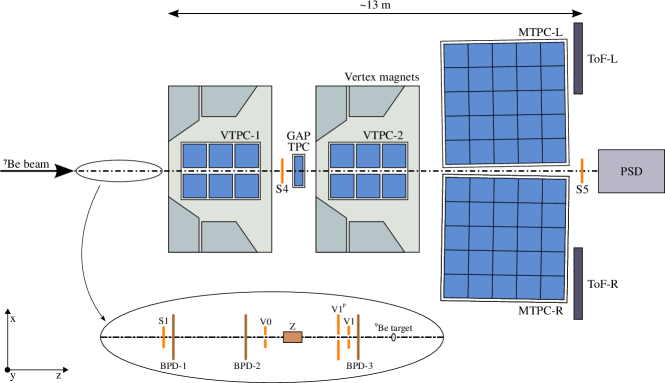
Figure 1: Schematic of the NA61/SHINE detector setup, used during the Be+Be data taking.

3.1 Detectors

The key components of the experiment for the detection of particles produced in the collisions are the five large volume Time Projection Chambers (TPCs) for tracking. The two most upstream ones are the Vertex TPCs (VTPCs), residing in the two superconducting bending magnets. The magnets have 9 T$\cdot$m maximum combined bending power. Downstream of the VTPCs, the two Main TPCs (MTPCs) are located symmetrically to the beam line in order to extend the tracking lever arm and to perform particle identification by measuring their ionisation energy loss in the TPC gas. One smaller TPC is located in the gap between VTPCs, and is called Gap-TPC (GTPC; denoted GAP TPC in Fig. 1). The VTPCs and GTPC are operated with an Ar(90):CO₂(10) gas mixture and the MTPCs with an Ar(95):CO₂(5) mixture. The further downstream Time-of-Flight (ToF) detectors are not used in the present analysis.

The Projectile Spectator Detector (PSD) at the end of the setup is a segmented forward hadron calorimeter, centered on the nominal deflected beam trajectory. It measures the energy contained in the projectile spectators which is used for event centrality characterization.

The beam line instrumentation is schematically shown in the inset of Fig. 1. A set of scintillation counters as well as beam position detectors (BPDs) [7] upstream of the target provide timing reference, selection, identification and precise measurement of the position and direction of individual beam particles.

3.2 Triggers

The schematic of the placement of the beam and trigger detectors is shown in the inset of Fig. 1. These consist of a scintillation counter (S1) recording the presence of the beam particle, a set of veto scintillation counters with hole (V0, V1, V1^p) used for rejecting beam halo particles, and a threshold Cherenkov charge detector (Z). Trigger signals indicating the passage of valid beam particles are defined by the coincidence T1 = $\text{S1}\cdot\overline{\text{V0}}\cdot\overline{\text{V1}}\cdot\overline{\text{V1${}^{p}$}}\cdot\text{Z(Be)}$ for high momentum data taking.

Central collisions were selected through the analysis of the signal from the 16 central modules of the PSD [49]. The low-energy part of the deposited energy spectrum was selected to contain 20% of the most central collisions. The interaction trigger condition was thus T2 = T1$\cdot\overline{\text{PSD}}$ for the higher energies.

The data consists of $\approx 2{.}828\cdot 10^{6}$ events before event and track selection.

3.3 The ⁷Be beam and ⁹Be target

The NA61/SHINE beamline is designed to handle primary as well as secondary beams. The beam instrumentation was optimized accordingly. In the Be+Be runs, a secondary beam was used, fragmented from a primary Pb beam from the SPS accelerator. A threshold Cherenkov charge tagging detector, called the Z detector, was used in order to identify and select the $Z=4$ fragment nuclei. In order to have a low material budget for the Z detector, a thin quartz wafer Cherenkov radiator was used. Additionally, the amplitudes of the signals measured in the three Beam Position Detectors (BPDs, see Fig. 1) were used to improve the Z resolution. A detailed description of the technique for the identification of ⁷Be fragments is given in Ref. [18].

The target was a 12 mm thick plate of ⁹Be placed approximately 80.0 cm upstream of VTPC-1. The total mass concentrations of impurities in the target were measured at 0.287%  [50]. No correction was applied for this negligible contamination.

4 Analysis procedure

Bose-Einstein correlations are studied in this paper for pions reconstructed as originating from the primary interaction in the 20% most central ⁷Be+⁹Be collisions as selected by the total energy emitted into the forward direction covered by the PSD detector. In the following, we describe the event, track and pair selection procedure, and all the steps required to obtain the measured source parameters.

4.1 Event selection

The events considered for analysis had to satisfy the following conditions:

1. no off-time beam particle detected within a time window of $4.5\leavevmode\nobreak\ \mu$s around the particle triggering the event,

2. event has a well-fitted main interaction vertex,

3. the maximal distance between the main vertex $z$ position and the centre of the beryllium target is between $\pm$ 5 cm,

4. the 0–20% most central collisions, based on PSD energy measurement, are accepted.

4.2 Track selection

The tracks selected for the analysis had to satisfy the following conditions:

1. the fit of particle track converged,

2. the distance between the track extrapolated to the interaction plane and the interaction point (impact parameter) should be smaller or equal to 4 cm in the horizontal (bending – $|B_{x}|$) plane and 2 cm in the vertical (drift – $|B_{y}|$) plane,

3. the total number of reconstructed points in all TPCs on the track should be at least 30 and, at the same time, the sum of the number of reconstructed points in VTPC-1 and VTPC-2 should be at least 15 or the number of reconstructed points in the GTPC should be at least 5,

4. the ratio of total number of reconstructed points on the track to the potential number of points should be between 0.5 and 1.0 (nPointRatio),

5. identified particle’s rapidity is in the interval $\pm 2$ around midrapidity.

4.3 Particle identification

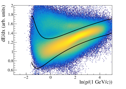
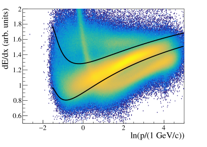
Figure 2: The ${\textrm{d}}E\!/\!{\textrm{d}}x$ measurement for negatively charged (left panel) and positively charged (right panel) particles versus natural logarithm of momentum $p$ (in laboratory frame). The two lines represent the interpolated selection boundaries based on Gaussian fits to ${\textrm{d}}E\!/\!{\textrm{d}}x$ distributions at several momenta, and are 3 standard deviations from the pion mean for negatively charged particles, while for positively charged particles, the lower line is 1.5 standard deviations distance from the mean, to remove the more significant kaon and proton contributions present in this case.

Particle identification (PID) for pions was performed using ${\textrm{d}}E\!/\!{\textrm{d}}x$ cuts, shown in Fig. 2. The contribution between the two lines are considered pions. The fine-tuning of the ${\textrm{d}}E\!/\!{\textrm{d}}x$ cut parameters was performed as follows.

1. a reasonable interval in $\log(p/1(\textnormal{GeV}/c)$ was selected where the pion contribution dominates (from -1.6 to 4,  0.2 to  55 $\mbox{Ge\kern-1.00006ptV}\!/\!c$),

2. the data was binned in $\log(p)$ into 80 slices,

3. in each bin a Gaussian was fitted to the ${\textrm{d}}E\!/\!{\textrm{d}}x$ data, in order to establish the most probable value of the pion ${\textrm{d}}E\!/\!{\textrm{d}}x$ peak,

4. the standard deviation ($\sigma$) obtained from these Gaussian fits was used to determine the pion ${\textrm{d}}E\!/\!{\textrm{d}}x$ response width (found to be between 0.05 and 0.18, depending on momentum), which was the basis of the pion ${\textrm{d}}E\!/\!{\textrm{d}}x$ selection as shown in Fig. 2.

4.4 Pair selection and event mixing

Due to the possible imperfections of the detector and of the tracking algorithm, hits created by a single particle may be reconstructed as two tracks. This is called track splitting and leads to a track pair with small momentum difference (< 20 $\mbox{Me\kern-1.00006ptV}/c$). Furthermore, the hits of two close particles may be reconstructed as a single track: this is called track merging. In a correlation analysis, it is important to minimize the effect of these track reconstruction problems. Track splitting is already largely removed by the track selection cuts (in particular, (iv) of Sec. 4.2). The contribution from track merging was estimated by Monte Carlo (MC) simulations using EPOS simulation [51] and GEANT3 for particle propagation [52] and reconstruction, and an appropriate lower limit in the momentum difference was defined, as described below.

The basic quantity of correlation measurements is the pair distribution. From pairs of pions created in the same event, one obtains the so-called actual pair distribution $A(q)$. Such distributions were measured in several intervals of average pair transverse momentum $K_{T}$ or pair transverse mass $m_{\textnormal{T}}$. This pair distribution is influenced by single-particle momentum distributions, kinematic acceptance of the detector, phase-space effects and other phenomena, not connected to quantum-statistics or final state interactions. These can be removed by constructing a combinatorial background pair distribution $B(q)$, measured in the same $K_{T}$ or $m_{\textnormal{T}}$ intervals as the $A(q)$ distribution. Calculating this background distribution starts with the event mixing procedure, where an artificial, mixed event is created from particles originating from different events. Subsequently, pairs formed within the mixed event are used to create the background distribution $B(q)$. By construction, this method ensures that no two particles are selected from the same background event, minimizing residual (non-quantum-statistical) correlations.

The obtained background distribution $B(q)$ exhibits all the previously mentioned non-quantum-statistical effects (acceptance, momentum distribution, phase-space, etc.), hence dividing $A(q)$ by $B(q)$ leaves us with a ratio which exhibits quantum-statistical and final-state interaction effects as well as the effect of reconstruction inefficiencies (and, in addition, momentum conservation, which is not relevant in the range of the investigated $q$-range). Thus, the measured correlation function is defined as

$$C_{2}(q)=\frac{A(q)}{B(q)}\cdot\frac{\int_{q_{1}}^{q_{2}}B(q)dq}{\int_{q_{1}}^{q_{2}}A(q)dq},$$ (19)

where [$q_{1},q_{2}$] is a large-$q$ range where quantum-statistical effects are no longer affecting the correlation function. The integrals in Eq. (19) provide the normalization of the correlation function to unity at high relative momentum. An example for $C_{2}(q)$ is shown in Fig. 3 for both data and EPOS simulation. It is readily apparent that at low $q$ values Bose-Einstein correlation and Coulomb repulsion effects determine $C_{2}(q)$ data points. These effects are not present in the simulations, hence the simulated $C_{2}(q)$ values are approximately constant. The reconstructed $C_{2}(q)$ however suffers from track merging effects (where the two tracks forming the pairs are close spatially), strongly suppressing $C_{2}(q)$ at low $q$ values. Hence the deviation of the simulated and reconstructed correlation function provides a good estimate of the range where inefficiencies are important. This allows to determine the range in $q$ over which fits can be considered reliable. The fit range is then selected for each $K_{\textnormal{T}}$ bin, e.g. for $K_{\textnormal{T}}=0.20-0.35$ $\mbox{Ge\kern-1.00006ptV}\!/\!c$ the interval where fit is considered good is $q=0.049-0.8$ $\mbox{Ge\kern-1.00006ptV}\!/\!c$.

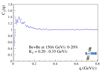
Figure 3: The ratio of $A(q)$ and $B(q)$ as a function of $q$. Left: measured NA61/SHINE data. Right: EPOS simulation and EPOS reconstructed data (GEANT3 + NA61/SHINE rec. chain).

4.5 Estimation of source shape parameters via fitting

The measured correlations were fitted with the formula described in Eq. (16). Due to the often modest number of entries in the signal and background distributions [53], Poisson maximum-likelihood fitting was used [54]. The corresponding penalty function ($\chi^{2}_{\lambda,p}$) to minimise is

$$\chi^{2}_{\lambda,p}=2\Big{[}\sum_{i}\Big{(}y_{i}-n_{i}\Big{)}+\Big{(}\sum_{\mathclap{\begin{subarray}{c}i\\ c_{i}\neq 0\end{subarray}}}n_{i}\cdot\ln(n_{i}/y_{i})\Big{)}\Big{]},$$ (20)

where $\lambda$ and $p$ denote the fact that we are using a likelihood $\chi^{2}$ for Poisson distributed histograms, $c_{i}$ references the number of counts, $n_{i}$ is the number of entries in the i^th histograming bin obtained from the data, and $y_{i}$ is its corresponding parametric model value to be fitted to the data. Goodness-of-fit was determined using regular $\chi^{2}$ methods in two ranges: the full range and the Bose-Einstein peak range. Fits were done both for positively and negatively charged pion pairs, as well as their combinations, in four $m_{\textnormal{T}}$ intervals. A fit was accepted if the algorithm converged, the covariance matrix was positive definite, and the confidence value corresponding to the $\chi^{2}\textnormal{ and NDF}$ was larger than 0.1%. An example fit is shown in Fig. 4. To estimate the statistical uncertainties of the fit parameters, the Minos method was utilised  [55] (also called as likelihood based confidence intervals) which by its nature, yields asymmetric statistical errors.

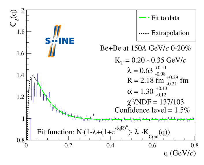
Figure 4: Example fit with Bose-Einstein correlation function at $K_{T}=0.20-0.35$ $\mbox{Ge\kern-0.90005ptV}\!/\!c$ for the sum $\left(\pi^{+}+\pi^{+}\right)+\left(\pi^{-}+\pi^{-}\right)$. The green line shows the fitted function with Coulomb correction given by Eq. (16) within the range of 0.049 $\mbox{Ge\kern-0.90005ptV}\!/\!c$ to 0.8 $\mbox{Ge\kern-0.90005ptV}\!/\!c$.

4.6 Systematic uncertainties

In the analysis one has to consider that the parameters obtained from fits depend on several experimental choices and cuts, such as the PID cut, the width of bins or the fitting range. These dependencies are the dominating contributors to the systematic uncertainties. In order to estimate these, the fits were performed with loose and tight event and track selection criteria, and also with slightly varied fit intervals. The standard set of cut values together with the alternative values for systematic error estimation are shown in Table 1. The systematic uncertainty calculation was performed for positively and negatively, like-sign charged pairs summed together.

n	Source	standard	tight	loose
0	nPoint	$\geq 30$	$\geq 40$	$\geq 10$
1	nPointRatio	$0.5-1.0$	$0.7-1.0$	$0.4-1.2$
2	VTPC points	$\geq 15$	$\geq 30$	$>10$
3	GTPC points	$\geq 5$	$\geq 5$	$>6$
4	$|B_{x}|$ $|B_{y}|$	$\leq 4$ cm $\leq 2$ cm	$\leq 0.8$ cm $\leq 0.8$ cm	$\leq 6$ cm $\leq 5$ cm
5	$q$ bin width	7 MeV/$c$	3.5 MeV/$c$	3.5 MeV/$c$
6	Fit range	$K_{T}$ dependent, lower value is from MC
7	PID cut	$\pi^{+}$: +3$\sigma$ and -1.5$\sigma$ $\pi^{-}$: +3$\sigma$ and -3$\sigma$	$\pi^{+}$: +2$\sigma$ and -1$\sigma$, $\pi^{-}$: +2$\sigma$ and -2$\sigma$	$\pi^{+}$: +4$\sigma$ and -2$\sigma$ $\pi^{-}$: +4$\sigma$ and -4$\sigma$
8	vertex $z$ (cm)	-585– -575	-585– -575	-595 – -565

Table 1: The standard cuts used to obtain the final results, as well as the loose and tight cuts applied for estimation of systematic uncertainties.

The combined systematic uncertainties were obtained as follows. Let $P$ denote the fit parameter vector ($\alpha,\lambda,R$). Denote by $P_{n}^{j}(i)$ the corresponding estimated parameter vector obtained for the $i$-th $m_{T}$ bin ($i=0,\dots,3$), with the $n$-th selection criterion ($n=0,\dots,8$) listed in Table 1 set to the $j$-th setting ($j=0,1,2$ meaning the standard, tight and loose values). The downward ($\delta P^{-}$) and upward ($\delta P^{+}$) systematic uncertainty of the parameter vector $P$ was estimated as follows:

$$\delta P^{+}(i)=\sqrt{\sum_{n}\frac{1}{N^{j+}_{n}}\sum_{j\epsilon J_{n}^{+}}(P_{n}^{j}(i)-P^{0}(i))^{2}},$$ (21)

$$\delta P^{-}(i)=\sqrt{\sum_{n}\frac{1}{N^{j-}_{n}}\sum_{j\epsilon J_{n}^{-}}(P_{n}^{j}(i)-P^{0}(i))^{2}},$$ (22)

where $P^{0}(i)$ is the parameter vector in $i$-th $m_{T}$ bin with standard cut ($j=0$), $J_{n}^{+}$ and $J_{n}^{-}$ are the array of $j$ values with which $P^{j}_{n}(i)>P^{0}(i)\textnormal{, and }P^{j}_{n}(i)<P^{0}(i)$ occurs respectively, and $N^{j+}_{n}\textnormal{ and }N^{j-}_{n}$ denote their corresponding multiplicity.

5 Results

The three physical parameters ($\alpha,\;\lambda\;\textnormal{and}\;R$) were measured in four bins of pair transverse momentum $K_{T}$ or pair transverse mass $m_{T}$. The parameters were obtained via fitting a parametric Lévy ansatz on the source via the formula Eq. (16) to the measured correlation functions.

The transverse mass dependence of the intercept parameter $\lambda$ is shown in Fig. 5. One may observe, within uncertainties, $\lambda(m_{T})\approx$ const. in the available $m_{T}$ range. When compared to measurements at RHIC energy Au+Au collisions [24, 56, 57] and at SPS energy Pb+Pb collisions [58, 59], an interesting phenomenon becomes apparent. At the SPS energies, there is no visible decrease of $\lambda$ at lower $m_{T}$ values, but at RHIC energies, a “hole” appears at $m_{T}$ values arond 2-300 MeV. This “hole” was interpreted in Ref. [24, 60] to be a sign of in-medium mass modification of the $\eta^{\prime}$ meson. The NA61/SHINE results do not indicate the presence of a low-$m_{T}$ hole. Furthermore, it is important to note that the obtained values for $\lambda$ are smaller than unity, which in the framework of the core-halo model may indicate that a significant fraction of pions are the decay products of long-lived resonances.

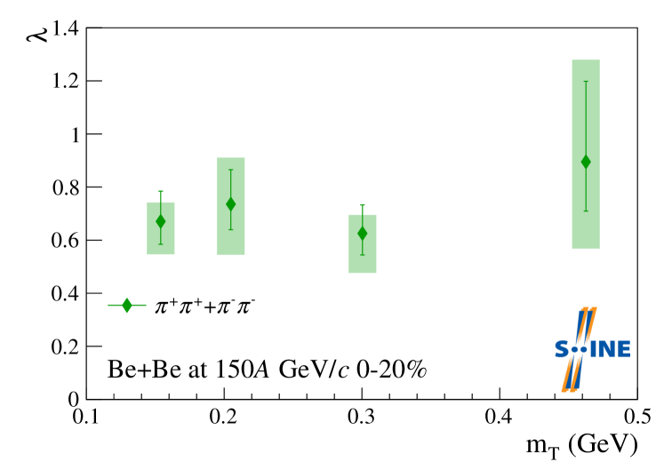
Figure 5: The intercept parameter $\lambda$, for 0–20% central Be+Be at 150$A\,\mbox{Ge\kern-0.90005ptV}\!/\!c$, as a function of $m_{T}$. Boxes denote systematic uncertainties, bars represent statistical ones.

The measured values of the radial scale parameter $R$ of the Lévy shaped source function, determining the homogeneity length of the pion emitting source in the LCMS, are shown in Fig. 6 as a function of $m_{T}$. Interestingly, the resulting $R$ parameter values are similar to those measured in p+p collisions at the CMS [33, 61]. We also observe a slight decrease of $R$ with increasing $m_{T}$. This can be explained by the presence of radial flow, based on simple hydrodynamical models [62, 63] where one obtains a $1/R^{2}\propto m_{T}$ type of transverse mass dependence:

$$R=\frac{A}{\sqrt{1+m_{T}/B}}.$$ (23)

This function was fitted to the $R$ values measured in each $m_{\textnormal{T}}$ bin, as shown in Fig. 6, resulting in a good fit quality ($\chi^{2}/\textnormal{NDF}=1.7/2$, corresponding to a confidence level of 44%). The obtained fit parameters are: $A=4.5\pm 2.9$ (stat.) fm and $B=0.12\pm 0.23$ (stat.) GeV, comparable to those measured in p+p collisions at CMS [61] (although the large uncertainties prevent a quantitative comparison).

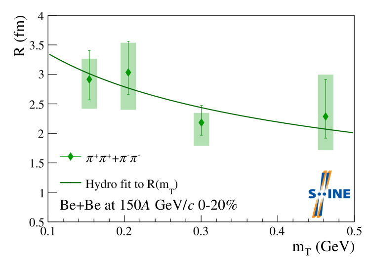
Figure 6: The radial scale parameter $R$, for 0–20% central Be+Be at 150$A\,\mbox{Ge\kern-0.90005ptV}\!/\!c$, as a function of $m_{T}$. The fit to $R(m_{T})$ with Eq. (23) is shown with a solid line. Boxes denote systematic uncertainties, bars represent statistical ones.

The Lévy stability exponent $\alpha$ describes the shape of the tail of the source distribution. The NA61/SHINE results, shown in Fig. 7, yield values for $\alpha$ between 0.9 and 1.5, and are significantly lower than the Gaussian ($\alpha=2$) case, and also significantly higher than the conjectured critical endpoint value ($\alpha=0.5$). The obtained $\alpha$ values are in a similar range as the ones obtained in Au+Au collisions at RHIC energies [24]. The shape of the pion emitting source is apparently independent of $m_{T}$, within uncertainties. Therefore one can calculate a simple average of the four $\alpha$ values via a constant fit, shown in Fig. 7, and resulting in a good fit quality ($\chi^{2}/\textnormal{NDF}=6.0/2$, corresponding to a confidence level of 11%). This results in an average value of $\overline{\alpha}=1.07\pm 0.06$ (stat.) which describes a source shape close to a Cauchy distribution (where $\alpha=1$). Further studies are foreseen at NA61/SHINE using different collision energies and system sizes in order to map the evolution of the Lévy stability index $\alpha$ as a function of collision energy and system size.

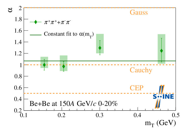
Figure 7: The Lévy stability index $\alpha$, for 0–20% central Be+Be at 150$A\,\mbox{Ge\kern-0.90005ptV}\!/\!c$, as a function of $m_{T}$. Special cases corresponding to a Gaussian ($\alpha=2$) or a Cauchy ($\alpha=1$) source are shown, as well as $\alpha=0.5$, the conjectured value corresponding to the critical endpoint, while the constant $\alpha$ fit is shown with a solid line. Boxes denote systematic uncertainties, bars represent statistical ones.

6 Summary and conclusions

Measurement of two-particle Bose-Einstein correlations in 150$A\,\mbox{Ge\kern-1.00006ptV}\!/\!c$ Be+Be collisions with the NA61/SHINE detector system were presented. The correlation functions were measured in several bins of pair transverse mass $m_{T}$, and their fundamental shape parameters were extracted via fitting a Lévy shaped ansatz for the particle source function. Correction for the final state Coulomb interaction was performed. The $m_{T}$-dependence of the shape parameters $\lambda$, $R$ and $\alpha$ were studied.

The results show that the Lévy exponent $\alpha$ is approximately constant as a function of $m_{T}$, and far from both the Gaussian case of $\alpha=2$ or the conjectured value at the critical endpoint, $\alpha=0.5$. The radius scale parameter $R$ shows a slight decrease in $m_{T}$, which can be explained as a signature of transverse flow. Finally, an approximately constant trend of the intercept parameter $\lambda$ as a function of $m_{T}$ was observed, clearly different from measurement results at RHIC. The NA61/SHINE experimental program plans further measurements at different energies and system sizes of these Lévy shape parameters. This will complete a systematic study of the energy and system size dependence of the source shape parameters.

The NA61/SHINE Collaboration

H. Adhikary¹³, P. Adrich¹⁵, K.K. Allison²⁹, N. Amin⁵, E.V. Andronov²⁵, T. Antićić³, I.-C. Arsene¹², M. Bajda¹⁶, Y. Balkova¹⁸, M. Baszczyk¹⁷, D. Battaglia²⁸, A. Bazgir¹³, S. Bhosale¹⁴, M. Bielewicz¹⁵, A. Blondel⁴, M. Bogomilov², Y. Bondar¹³, N. Bostan²⁸, A. Brandin²⁴, W. Bryliński²¹, J. Brzychczyk¹⁶, M. Buryakov²³, A.F. Camino³¹, M. Ćirković²⁶, M. Csanád⁸, J. Cybowska²¹, T. Czopowicz^13,21, C. Dalmazzone⁴, N. Davis¹⁴, A. Dmitriev ²³, P. von Doetinchem³⁰, W. Dominik¹⁹, P. Dorosz¹⁷, J. Dumarchez⁴, R. Engel⁵, G.A. Feofilov²⁵, L. Fields²⁸, Z. Fodor^7,20, M. Friend⁹, A. Garibov¹, M. Gaździcki^13,6, O. Golosov²⁴, V. Golovatyuk ²³, M. Golubeva²², K. Grebieszkow²¹, F. Guber²², S.N. Igolkin²⁵, S. Ilieva², A. Ivashkin²², A. Izvestnyy²², K. Kadija³, N. Kargin²⁴, N. Karpushkin²², E. Kashirin²⁴, M. Kiełbowicz¹⁴, V.A. Kireyeu²³, H. Kitagawa¹⁰, R. Kolesnikov²³, D. Kolev², Y. Koshio¹⁰, V.N. Kovalenko²⁵, S. Kowalski¹⁸, B. Kozłowski²¹, A. Krasnoperov²³, W. Kucewicz¹⁷, M. Kuchowicz²⁰, M. Kuich¹⁹, A. Kurepin²², A. László⁷, M. Lewicki²⁰, G. Lykasov²³, V.V. Lyubushkin²³, M. Maćkowiak-Pawłowska²¹, Z. Majka¹⁶, A. Makhnev²², B. Maksiak¹⁵, A.I. Malakhov²³, A. Marcinek¹⁴, A.D. Marino²⁹, K. Marton⁷, H.-J. Mathes⁵, T. Matulewicz¹⁹, V. Matveev²³, G.L. Melkumov²³, A. Merzlaya¹², Ł. Mik¹⁷, A. Morawiec¹⁶, S. Morozov²², Y. Nagai⁸, T. Nakadaira⁹, M. Naskręt²⁰, S. Nishimori⁹, V. Ozvenchuk¹⁴, O. Panova¹³, V. Paolone³¹, O. Petukhov²², I. Pidhurskyi^13,6, R. Płaneta¹⁶, P. Podlaski¹⁹, B.A. Popov^23,4, B. Pórfy^7,8, M. Posiadała-Zezula¹⁹, D.S. Prokhorova²⁵, D. Pszczel¹⁵, S. Puławski¹⁸, J. Puzović²⁶, R. Renfordt¹⁸, L. Ren²⁹, V.Z. Reyna Ortiz¹³, D. Röhrich¹¹, E. Rondio¹⁵, M. Roth⁵, Ł. Rozpłochowski¹⁴, B.T. Rumberger²⁹, M. Rumyantsev²³, A. Rustamov^1,6, M. Rybczynski¹³, A. Rybicki¹⁴, K. Sakashita⁹, K. Schmidt¹⁸, A.Yu. Seryakov²⁵, P. Seyboth¹³, U.A. Shah¹³, Y. Shiraishi¹⁰, A. Shukla³⁰, M. Słodkowski²¹, P. Staszel¹⁶, G. Stefanek¹³, J. Stepaniak¹⁵, M. Strikhanov²⁴, H. Ströbele⁶, T. Šuša³, Ł. Świderski¹⁵, J. Szewiński¹⁵, R. Szukiewicz²⁰, A. Taranenko²⁴, A. Tefelska²¹, D. Tefelski²¹, V. Tereshchenko²³, A. Toia⁶, R. Tsenov², L. Turko²⁰, T.S. Tveter¹², M. Unger⁵, M. Urbaniak¹⁸, F.F. Valiev²⁵, D. Veberič⁵, V.V. Vechernin²⁵, V. Volkov²², A. Wickremasinghe²⁷, K. Wójcik¹⁸, O. Wyszyński¹³, A. Zaitsev²³, E.D. Zimmerman²⁹, A. Zviagina²⁵, and R. Zwaska²⁷

¹ National Nuclear Research Center, Baku, Azerbaijan
² Faculty of Physics, University of Sofia, Sofia, Bulgaria
³ Ruđer Bošković Institute, Zagreb, Croatia
⁴ LPNHE, University of Paris VI and VII, Paris, France
⁵ Karlsruhe Institute of Technology, Karlsruhe, Germany
⁶ University of Frankfurt, Frankfurt, Germany
⁷ Wigner Research Centre for Physics, Budapest, Hungary
⁸ Eötvös Loránd University, Budapest, Hungary
⁹ Institute for Particle and Nuclear Studies, Tsukuba, Japan
¹⁰ Okayama University, Japan
¹¹ University of Bergen, Bergen, Norway
¹² University of Oslo, Oslo, Norway
¹³ Jan Kochanowski University, Poland
¹⁴ Institute of Nuclear Physics, Polish Academy of Sciences, Cracow, Poland
¹⁵ National Centre for Nuclear Research, Warsaw, Poland
¹⁶ Jagiellonian University, Cracow, Poland
¹⁷ AGH - University of Science and Technology, Cracow, Poland
¹⁸ University of Silesia, Katowice, Poland
¹⁹ University of Warsaw, Warsaw, Poland
²⁰ University of Wrocław, Wrocław, Poland
²¹ Warsaw University of Technology, Warsaw, Poland
²² Institute for Nuclear Research, Moscow, Russia
²³ Joint Institute for Nuclear Research, Dubna, Russia
²⁴ National Research Nuclear University (Moscow Engineering Physics Institute), Moscow, Russia
²⁵ St. Petersburg State University, St. Petersburg, Russia
²⁶ University of Belgrade, Belgrade, Serbia
²⁷ Fermilab, Batavia, USA
²⁸ University of Notre Dame, Notre Dame , USA
²⁹ University of Colorado, Boulder, USA
³⁰ University of Hawaii at Manoa, USA
³¹ University of Pittsburgh, Pittsburgh, USA

References

- [1] R. Hanbury Brown and R. Q. Twiss Nature 178 (1956) 1046.
- [2] G. Goldhaber, W. B. Fowler, S. Goldhaber, and T. F. Hoang Phys. Rev. Lett. 3 (1959) 181.
- [3] G. Goldhaber, S. Goldhaber, W.-Y. Lee, and A. Pais Phys. Rev. 120 (1960) 300.
- [4] S. S. Adler et al., [PHENIX Collab.] Phys. Rev. Lett. 93 (2004) 152302, arXiv:nucl-ex/0401003.
- [5] S. Afanasiev et al., [PHENIX Collab.] Phys. Rev. Lett. 103 (2009) 142301.
- [6] T. Csörgő, S. Hegyi, T. Novák, and W. A. Zajc AIP Conf. Proc. 828 no. 1, (2006) 525–532, arXiv:nucl-th/0512060.
- [7] N. Abgrall et al., [NA61/SHINE Collab.] JINST 9 (2014) P06005, arXiv:1401.4699 [physics.ins-det].
- [8] M. Gazdzicki, Z. Fodor, G. Vesztergombi, et al., [NA49-future Collab.], “Study of Hadron Production in Hadron-Nucleus and Nucleus-Nucleus Collisions at the CERN SPS,” Tech. Rep. CERN-SPSC-2006-034, SPSC-P-330, CERN, Geneva, Nov, 2006. https://cds.cern.ch/record/995681.
- [9] F. Becattini, J. Manninen, and M. Gazdzicki Phys.Rev. C73 (2006) 044905, arXiv:hep-ph/0511092 [hep-ph].
- [10] V. Vovchenko, V. V. Begun, and M. I. Gorenstein Phys. Rev. C 93 no. 6, (2016) 064906, arXiv:1512.08025 [nucl-th].
- [11] A. Aduszkiewicz et al., [NA61/SHINE Collab.], “Beam momentum scan with Pb+Pb collisions,” Tech. Rep. CERN-SPSC-2015-038, SPSC-P-330-ADD-8, CERN, Geneva, Oct, 2015. https://cds.cern.ch/record/2059811.
- [12] N. Abgrall et al., [NA61/SHINE Collab.] Eur.Phys.J. C74 (2014) 2794, arXiv:1310.2417 [hep-ex].
- [13] A. Aduszkiewicz et al., [NA61/SHINE Collab.] Eur. Phys. J. C 77 no. 10, (2017) 671, arXiv:1705.02467 [nucl-ex].
- [14] A. Aduszkiewicz et al., [NA61/SHINE Collab.] Phys. Rev. C 102 no. 1, (2020) 011901, arXiv:1912.10871 [hep-ex].
- [15] A. Acharya et al., [NA61/SHINE Collab.] Eur. Phys. J. C 81 no. 5, (2021) 397, arXiv:2101.08494 [hep-ex].
- [16] A. Acharya et al., [NA61/SHINE Collab.] Eur. Phys. J. C 81 no. 1, (2021) 73, arXiv:2010.01864 [hep-ex].
- [17] A. Acharya et al., [NA61/SHINE Collab.] Eur. Phys. J. C 80 no. 10, (2020) 961, arXiv:2008.06277 [nucl-ex]. [Erratum: Eur.Phys.J.C 81, 144 (2021)].
- [18] N. Abgrall et al., [NA61/SHINE Collab.], “The 2010 test of secondary light ion beams,” Tech. Rep. CERN-SPSC-2011-005, SPSC-SR-077, CERN, Geneva, Jan, 2011. https://cds.cern.ch/record/1322135.
- [19] S. Pratt, T. Csörgő, and J. Zimányi Phys. Rev. C 42 (1990) 2646–2652.
- [20] T. Csörgő Acta Phys. Hung. A 15 (2002) 1–80, arXiv:hep-ph/0001233.
- [21] M. A. Lisa, S. Pratt, R. Soltz, and U. Wiedemann Ann. Rev. Nucl. Part. Sci. 55 (2005) 357–402, arXiv:nucl-ex/0505014.
- [22] S. S. Adler et al., [PHENIX Collab.] Phys. Rev. Lett. 93 (2004) 152302, arXiv:nucl-ex/0401003.
- [23] S. Bekele et al. Braz. J. Phys. 37 (2007) 31, arXiv:0706.0537 [nucl-ex].
- [24] A. Adare et al., [PHENIX Collab.] Phys. Rev. C 97 no. 6, (2018) 064911, arXiv:1709.05649 [nucl-ex].
- [25] J. Adamczewski-Musch et al., [HADES Collab.] Eur. Phys. J. A 56 no. 5, (2020) 140, arXiv:1910.07885 [nucl-ex].
- [26] J. Bolz, U. Ornik, M. Plumer, B. R. Schlei, and R. M. Weiner Phys. Rev. D 47 (1993) 3860–3870.
- [27] T. Csörgő, B. Lörstad, and J. Zimányi Z. Phys. C 71 (1996) 491–497, arXiv:hep-ph/9411307.
- [28] R. M. Weiner Phys. Rept. 327 (2000) 249–346, arXiv:hep-ph/9904389.
- [29] D. Kincses, M. I. Nagy, and M. Csanád Phys. Rev. C 102 no. 6, (2020) 064912, arXiv:1912.01381 [hep-ph].
- [30] T. Csörgő, S. Hegyi, and W. A. Zajc Eur. Phys. J. C 36 (2004) 67–78, arXiv:nucl-th/0310042.
- [31] R. Metzler, E. Barkai, and J. Klafter Phys. Rev. Lett. 82 (1999) 3563–3567.
- [32] P. Achard et al., [L3 Collab.] Eur. Phys. J. C 71 (2011) 1648, arXiv:1105.4788 [hep-ex].
- [33] A. M. Sirunyan et al., [CMS Collab.] Phys. Rev. C 97 no. 6, (2018) 064912, arXiv:1712.07198 [hep-ex].
- [34] [CMS Collab.], “Measurement of two-particle Bose-Einstein momentum correlations and their Levy parameters at TeV PbPb collisions,” Tech. Rep. CMS-PAS-HIN-21-011, CERN, Geneva, Apr, 2022. https://cds.cern.ch/record/2806150.
- [35] Y. Aoki, G. Endrodi, Z. Fodor, S. D. Katz, and K. K. Szabo Nature 443 (2006) 675–678, arXiv:hep-lat/0611014.
- [36] T. Bhattacharya et al. Phys. Rev. Lett. 113 no. 8, (2014) 082001, arXiv:1402.5175 [hep-lat].
- [37] R. A. Soltz, C. DeTar, F. Karsch, S. Mukherjee, and P. Vranas Ann. Rev. Nucl. Part. Sci. 65 (2015) 379–402, arXiv:1502.02296 [hep-lat].
- [38] T. Csörgő PoS HIGH-PTLHC08 (2008) 027, arXiv:0903.0669 [nucl-th].
- [39] A. M. Halasz, A. D. Jackson, R. E. Shrock, M. A. Stephanov, and J. J. M. Verbaarschot Phys. Rev. D 58 (1998) 096007, arXiv:hep-ph/9804290.
- [40] M. A. Stephanov, K. Rajagopal, and E. V. Shuryak Phys. Rev. Lett. 81 (1998) 4816–4819, arXiv:hep-ph/9806219.
- [41] S. El-Showk, M. F. Paulos, D. Poland, S. Rychkov, D. Simmons-Duffin, and A. Vichi J. Stat. Phys. 157 (2014) 869, arXiv:1403.4545 [hep-th].
- [42] H. Rieger Physical Review B 52 no. 9, (1995) 6659. http://link.aps.org/doi/10.1103/PhysRevB.52.6659.
- [43] M. Csanád, S. Lökös, and M. Nagy Phys. Part. Nucl. 51 no. 3, (2020) 238–242, arXiv:1910.02231 [hep-ph].
- [44] M. Csanád, S. Lökös, and M. Nagy Universe 5 no. 6, (2019) 133, arXiv:1905.09714 [nucl-th].
- [45] Y. Sinyukov, R. Lednicky, S. V. Akkelin, J. Pluta, and B. Erazmus Phys. Lett. B 432 (1998) 248–257.
- [46] M. G. Bowler Phys. Lett. B 270 (1991) 69–74.
- [47] R. Maj and S. Mrowczynski Phys. Rev. C 80 (2009) 034907, arXiv:0903.0111 [nucl-th].
- [48] B. Kurgyis, D. Kincses, M. Nagy, and M. Csanád arXiv:2007.10173 [nucl-th].
- [49] E. A. Kaptur, ”Analysis of collision centrality and negative pion spectra in 7Be+9Be interactions at CERN SPS energy range,” PhD Thesis, University of Silesia, Jun, 2017. https://edms.cern.ch/document/2004086/1.
- [50] D. Banas, A. Kubala-Kukus, M. Rybczynski, I. Stabrawa, and G. Stefanek Eur. Phys. J. Plus 134 no. 1, (2019) 44, arXiv:1808.10377 [nucl-ex].
- [51] T. Pierog and K. Werner Nucl.Phys.Proc.Suppl. 196 (2009) 102–105, arXiv:0905.1198 [hep-ph].
- [52] C. F. Brun R., “Geant detector description and simulation tool, cern program library long writeup w5013,” 1993. http://wwwasdoc.web.cern.ch/wwwasdoc/geant/geantall.html.
- [53] W. A. Zajc, J. Bistirlich, R. R. Bossingham, H. Bowman, C. Clawson, K. Crowe, K. Frankel, J. Ingersoll, J. Kurck, C. Martoff, et al. Phys. Rev. C 29 (Jun, 1984) 2173–2187. https://link.aps.org/doi/10.1103/PhysRevC.29.2173.
- [54] S. Baker and R. D. Cousins Nuclear Instruments and Methods in Physics Research 221 no. 2, (1984) 437–442.
- [55] W. Eadie, D. Drijard, F. James, M. Roos, and B. Sadoulet Journal of the American Statistical Association (07, 2013) .
- [56] R. Vértesi, T. Csörgő, and J. Sziklai Phys. Rev. C 83 (2011) 054903, arXiv:0912.0258 [nucl-ex].
- [57] B. I. Abelev et al., [STAR Collab.] Phys. Rev. C 80 (2009) 024905, arXiv:0903.1296 [nucl-ex].
- [58] H. Beker et al. Phys. Rev. Lett. 74 (1995) 3340–3343.
- [59] C. Alt et al., [NA49 Collab.] Phys. Rev. C 77 (2008) 064908, arXiv:0709.4507 [nucl-ex].
- [60] S. E. Vance, T. Csörgő, and D. Kharzeev Phys. Rev. Lett. 81 (1998) 2205–2208, arXiv:nucl-th/9802074.
- [61] A. M. Sirunyan et al., [CMS Collab.] JHEP 03 (2020) 014, arXiv:1910.08815 [hep-ex].
- [62] T. Csörgő and B. Lörstad Phys. Rev. C 54 (1996) 1390–1403, arXiv:hep-ph/9509213.
- [63] M. Csanád and M. Vargyas Eur. Phys. J. A 44 (2010) 473–478, arXiv:0909.4842 [nucl-th].