The 3D kinematics of stellar substructures in the periphery of the Large Magellanic Cloud

Abstract

We report the 3D kinematics of 27 Mira-like stars in the northern, eastern and southern periphery of the Large Magellanic Cloud (LMC), based on Gaia proper motions and a dedicated spectroscopic follow-up. Low-resolution spectra were obtained for more than 40 Mira-like candidates, selected to trace known substructures in the LMC periphery. Radial velocities and stellar parameters were derived for all stars. Gaia data release 3 astrometry and photometry were used to discard outliers, derive periods for those stars with available light curves, and determine their photometric chemical types. The 3D motion of the stars in the reference frame of the LMC revealed that most of the stars, in all directions, have velocities consistent with being part of the LMC disk population, out of equilibrium in the radial and vertical directions. A suite of N-body simulations was used to constrain the most likely past interaction history between the Clouds given the phase-space distribution of our targets. Model realizations in which the Small Magellanic Cloud (SMC) had three pericentric passages around the LMC best resemble the observations. The interaction history of those model realizations has a recent SMC pericentric passage ($\sim$320 Myr ago), preceded by an SMC crossing of the LMC disk at $\sim$0.97 Gyr ago, having a radial crossing distance of only $\sim$4.5 kpc. The previous disk crossing of the SMC was found to occur at $\sim$1.78 Gyr ago, with a much larger radial crossing distance of $\sim$10 kpc.

1 Introduction

The Magellanic Family is the poster child for binary dwarf galaxy collisions. Thanks to the advanced stage and overt intensity of the Clouds’ interaction, we have a rare opportunity to directly observe a variety of phenomena normally postulated to accompany and induce galaxy transformations. This includes tidal stripping and torquing, ram pressure gas removal, dynamical friction, and merger-induced star formation.

Several pieces of evidence in their morphologies reflect the intense past interaction history of this system. This includes, for example, the Large Magellanic Cloud (LMC) off-set stellar bar (Zhao & Evans, 2000; Choi et al., 2018), truncation of its outer stellar disk (Mackey et al., 2018), and the presence of warps (Olsen & Salyk, 2002; Choi et al., 2018). The past orbit of the Clouds suggests that they have experienced a recent close pericentric passage $\leq$250 Myr ago, consistent with the expected formation time of the Magellanic Bridge (Choi et al., 2018). Besides this ‘direct’ collision (impact parameter of $\lesssim$ 10 kpc), the details of previous interactions are not yet fully constrained.

In the periphery of the LMC, numerous stellar substructures – in the form of arms, clumps and streams – have been found thanks to wide-field deep-photometric surveys, as well as astrometric data from the Gaia mission. This plethora of substructure reflects its complex interaction history with the Small Magellanic Cloud (SMC) and/or the Milky Way. Towards the north, a thin and long stellar stream was first presented in Mackey et al. (2016), being subsequently studied in detail by several studies (e.g., Belokurov & Erkal, 2019; Gaia Collaboration et al., 2021; El Youssoufi et al., 2021; Cullinane et al., 2022a). Towards the east, a diffuse and extended stellar overdensity has been recovered based on different stellar tracers, receiving different names (e.g., ‘Eastern Substructure 1’, ‘Eastern Substructure 2’ El Youssoufi et al., 2021). Two thin stellar streams have been recovered towards the southern vicinity of the LMC, most likely embedded in a larger, diffuse stellar substructure (Belokurov & Erkal, 2019; El Youssoufi et al., 2021). The origin of these different stellar substructures around the Clouds is not yet established, although most of them are though to be part of the disturbed outer LMC disk based on the properties of their stellar populations and in-plane velocities.

Radial velocities, and with them, full 6D phase-space information for the stars in these substructures, is of paramount importance to understand their motions and to assess their possible origin. Up to date, a limited number of works have collected spectroscopic information for this purpose. In Cullinane et al. (2020), the Magellanic Edge Survey (MagES) is described, which collects multi-object spectroscopy of red giant branch and red clump stars. The MagES survey has analysed the northern arm (Cullinane et al., 2020), outer LMC stellar population (Cullinane et al., 2022b) and the SMC outskirts (Cullinane et al., 2023). Similarly, in Cheng et al. (2022) the results from APOGEE-2 observations in six fields towards the north and south of the LMC were presented.

While these previous observations were based on red giant branch and/or red clump stars, the errors on the proper motions of these stars tend to be larger than for the most luminous tracers. Moreover, at fields at larger distances from the LMC centre, contamination from Milky Way foreground stars can be non negligible. More luminous and less abundant tracers are thus well-suited to uncover the diffuse substructures in the LMC outskirts, as their contamination rate is smaller. Particularly, Deason et al. (2017) recovered several of the well-known stellar substructures around the LMC based on Mira-candidate stars. Being $\approx$ 3.5 mag brighter than red clump stars, moderate exposures times are require to derive reliable radial velocities. Motivated by this, we carried out a spectroscopic follow of more than 40 Mira-like stars in the vicinity of the Clouds, aiming to recover their phase-space information and use them to constrain the past interaction history of the Clouds.

This paper is organised as follows: in Section 2, a summary of the target selection for the spectroscopic follow-up is described. In Section 3, observations and data reduction are discussed. In Section 4, we present the spectroscopic analysis of our sample. Additional parameters such as parallax, periods, and heliocentric distances are discussed in Section 5. 3D cylindrical velocities in the LMC reference frame for the stars in the immediate LMC periphery are derived in Section 6. Finally, Section 7 presents a comparison between the observations and N-body simulations, while Section 8 presents the summary and conclusions of this work.

2 Target Selection

Candidate Mira variable stars were selected from Gaia DR1 data following the procedure outlined in Deason et al. (2017). In that work, repeated observations of sources during the initial phase of the Gaia mission were used to identify stars that show signs of variability. In particular, the Gaia ‘variability amplitude’ was used to identify stars that show signs of variability: $A=\sqrt{N_{\rm obs}}\sigma(F)/F$, where, $N_{\rm obs}$ is the number of CCD crossings, and $F$ and $\sigma(F)$ are the flux and flux error, respectively (see also Belokurov et al. 2017). This variability information was combined with infrared photometry from the Two Micron All Sky Survey (2MASS; Skrutskie et al., 2006) and the Wide field Infrared Survey Explorer (WISE; Wright et al., 2010) to select candidate giant stars in the vicinity of the LMC. For more details, please see Section 2 of Deason et al. (2017).

We select a sub-sample of these giant candidates for low-resolution spectroscopic follow-up to obtain radial velocities. In particular, we focus on the periphery of the Clouds, where there are interesting groups of stars to the East (‘Eastern excess’, EE), North (‘Mackey Stream’, MS), and South (possibly associated with the Leading Arm, dubbed ‘LA’) of the LMC. Figure 1 shows the location of the individual Mira-like stars observed, in a gnomonic (tangent-plane) projection, where the tangent point is located at the center of the LMC ($\alpha_{0}$, $\delta_{0}$) = (82$\aas@@fstack{\circ}$25, –69$\aas@@fstack{\circ}$5). All the Mira candidates from Deason et al. (2017) are shown as grey points. The locations of two previous spectroscopic campaigns around the periphery of the Clouds are included for reference (fields from Cullinane et al. 2022a and stars from Cheng et al. 2022). We also targeted some candidate giants away from the Magellanic Clouds (BP), which are above the disk plane (see Fig. 2). These could potentially be associated with Magellanic debris or distant halo stars with a different origin (see Section 5.4.2 for further discussion).

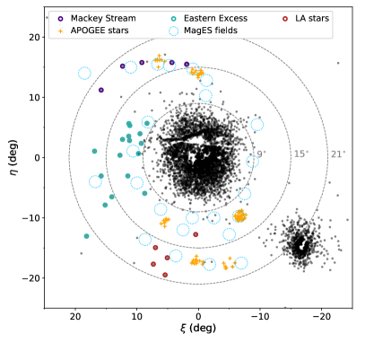
Figure 1: Mira candidates in the vicinity of the LMC and SMC, selected following the cuts detailed in Deason et al. (2017). The coordinates ($\eta$, $\xi$) are in the gnomonic (tangent-plane) projection. The dashed circles correspond to 9, 15 and 21° of angular separation from the LMC center. The targets selected for follow-up observations are marked with coloured circles, including five stars in the so-called Mackey Stream, 17 stars from the Eastern excess group, and five stars in the LA group. Blue unfilled circles mark the position of the fields in Cullinane et al. (2022b) while yellow crosses are individual stars from Cheng et al. (2022).

3 Observations and Data Reduction

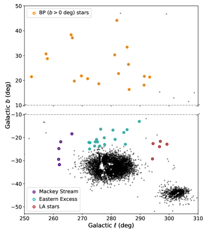
Figure 2: Galactic coordinate distribution of our target Mira stars. The three groups in the vicinity of the LMC and SMC (‘Mackey Stream’, ‘Eastern excess’ and ‘LA’) are the same targets as shown in Figure 1. The 17 target stars above the Galactic plane (‘BP’ group) are shown as orange open circles.

Mira candidates in the Magellanic periphery were observed for 4 nights with the COSMOS spectrograph (Martini et al., 2014) on the 4m Víctor Blanco telescope at Cerro Tololo Inter-American Observatory (CTIO). Long-slit spectra for 45 Miras were obtained using the Blue VPH Grism covering a wavelength range of 5600-9600 Å and a 1.0 arcsec slit, reaching a spectral resolution of $\sim$2000. Single exposures of 300s to 1800s per target were acquired, as well as one or two wavelength calibration arcs with Hg+Ne lamps observed at the same airmass as the targets. Radial velocity standard Miras (R Lep, HD 75021; Menzies et al., 2006) were also observed each night, with exposure times of 0.5 to 5 seconds.

A standard data reduction (flat-fielding, bias subtraction, extraction and wavelength calibration) was performed with the onespec package in IRAF (Tody, 1993). The lamps used were the non-standard Hg+Ne more suitable for calibration in the red part of the spectrum. A barycentric correction is then performed for each individual exposure, considering the Julian date, the place of the observatory on the surface of the Earth and the coordinates of each object.

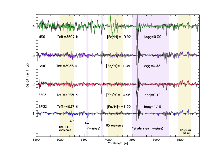
Figure 3: COSMOS spectra for a subsample of the observed targets together with the best fit derived with FERRE. The main stellar parameters derived for each target are also displayed. Yellow shadowed regions are for relevant regions (e.g., location of the Calcium triplet), while purple shadowed areas are those masked and not used for the FERRE fit.

Table 1: Mira variable candidate stars observed with the COSMOS spectrograph. Columns give the equatorial coordinates of the stars, radial velocities, and stellar parameters derived from the spectra (see Section 4). The last column gives the quality ’Flag’ for the derived stellar parameters, with flag=0 for those spectra where the spectroscopic fitting is unreliable.

ID	R.A.	Dec	Vrad	$\sigma_{\rm Vrad}$	Hemi	RV shift	[Fe/H]	Teff	logg	[Fe/H]CaT	Flag
	(hh:mm:ss.s)	(dd:mm:ss)	(km s-1)	(km s-1)	(Å)	(km s-1)		(K)	(cm s-2)
BP22	10:10:29.0	–31:44:53	320.39	6.71			–1.13	4091.71	0.68	–1.05	1
BP23	11:55:27.4	–39:57:44	158.24	9.55	6562.25	–25.04	–0.91	3939.74	0.81	–1.11	1
BP24	11:17:16.7	–36:20:11	324.31	7.60			–1.07	3834.37	0.00	–1.52	1
BP25	10:29:52.7	–33:29:26	39.59	10.69	6562.74	–2.79	–0.99	4013.93	0.49	–0.98	1
BP26	10:39:36.2	–37:08:53	109.06	9.56			–1.18	3747.15	0.00	–0.98	1
BP27	10:24:57.2	–31:25:47	313.41	10.67			–1.11	4039.59	0.38	–1.26	1
BP28	10:11:16.3	–17:41:28	156.86	43.82	6563.25	20.71	–2.93	3500.03	0.14	–3.85	0
BP29	11:21:35.3	–43:34:16	0.55	8.65			0.41	4145.97	5.00	0.03	1
BP30	10:54:28.0	–15:59:49	–10.04	9.01			–0.22	4205.23	5.00	0.50	1
			–13.13	8.34			–0.13	4186.30	5.00	0.50	1
BP31	11:49:21.1	–16:07:42	–3.22	9.86			–0.96	3919.75	4.79	–1.12	1
BP32	09:30:18.0	–21:04:54	234.58	10.70	6562.80	0.16	–1.30	4037.45	1.10	–1.69	1
BP33	10:07:07.0	–19:24:04	42.41	8.33			–0.86	3867.57	0.19	–0.98	1
BP34	10:52:49.4	–17:12:15	27.85	9.65			–0.81	3967.24	5.00	–0.01	1
BP35	11:25:38.0	–28:55:53	213.72	22.34	6562.71	–4.06	0.08	4491.12	1.28	–2.18	0
BP36	11:50:27.0	–43:22:29	162.73	86.68			–1.63	3545.06	1.91	–1.51	1
BP37	12:03:52.8	–40:37:26	235.83	23.03			0.23	4481.47	0.85	–1.91	0
BP38	11:37:54.5	–33:58:40	85.07	12.41			–1.01	3982.81	0.55	–1.02	1
BP39	11:45:58.0	–27:13:38	160.08	8.87	6562.46	–15.36	–2.48	3500.02	0.00	–2.68	1
EE06	08:49:19.0	–70:41:50	321.77	7.27			–0.96	3987.77	0.53	–1.00	1
EE07	07:43:44.4	–69:18:05	314.09	10.21			–1.05	3833.99	0.24	–1.64	1
EE08	07:36:51.5	–65:46:52	372.32	7.77			–0.96	4038.42	0.19	–0.96	1
EE09	06:59:30.5	–65:27:18	377.31	7.68			–0.96	3958.61	0.03	–0.94	1
EE10	07:33:06.8	–73:06:27	318.21	9.80			–1.66	3595.92	0.01	–1.07	1
EE11	07:09:52.1	–66:49:31	330.50	21.35			0.03	4496.49	1.28	–0.01	1
EE12	07:13:58.1	–64:19:10	341.07	7.83			–1.11	4020.17	0.59	–1.10	1
EE13	07:22:16.5	–63:42:15	295.71	13.47			0.14	4499.98	0.80	0.00	1
EE14	07:12:18.5	–63:38:09	260.53	80.62			–2.82	3500.01	2.47	–4.78	0
EE15	07:05:00.1	–62:06:39	325.72	13.57	6562.29	–23.48	–1.62	4066.17	1.62	–1.83	1
EE16	06:56:04.7	–63:54:41	279.11	61.28			–2.69	3500.26	0.00	–3.76	0
EE17	08:29:56.1	–70:29:23	182.25	41.15			–1.82	3500.13	1.73	–1.35	1
EE18	08:19:12.4	–66:53:22	162.79	10.26			–0.70	4035.83	0.84	–0.64	1
EE19	06:41:52.5	–62:38:53	312.61	7.92			–1.16	3895.31	0.40	–1.48	1
EE20	08:03:49.1	–63:08:30	357.66	10.26			–0.98	4036.74	0.22	–0.98	1
EE21	07:05:05.6	–61:45:39	381.97	10.93			–1.34	3680.01	0.04	–1.75	1
EE22	09:55:37.2	–71:13:39	150.92	8.40			–0.91	4083.29	1.30	–0.74	1
LA40	09:46:56.8	–82:16:36	248.70	7.78			–1.04	3935.65	0.33	–1.03	1
LA41	08:42:51.7	–83:30:38	220.52	6.90			–1.14	3770.16	0.00	–1.04	1
LA42	08:45:03.8	–81:04:20	269.10	7.26	6562.02	–35.47	–1.15	3831.63	1.10	–1.87	1
LA43	10:14:40.0	–84:36:22	94.74	12.44	6562.79	–0.27	–1.11	3959.30	0.75	–1.42	1
LA44	05:41:39.5	–82:03:02	220.28	10.71	6562.30	–22.95	–1.19	3809.93	1.25	–2.28	1
MS01	05:57:14.3	–53:54:02	317.07	21.15			–0.92	3507.28	0.00	–1.06	1
MS02	07:18:21.2	–55:19:44	254.90	53.34			0.46	4416.97	0.00	–2.96	0
MS03	06:48:06.4	–53:00:33	328.51	24.66	6562.71	–4.20	0.44	4441.20	0.00	–2.52	0
MS04	05:41:38.8	–54:20:09	276.47	13.71	6562.89	3.95	–1.26	3845.89	0.62	–1.92	1
			289.27	13.40	6562.74	–2.72	–1.25	3851.30	0.53	–2.01	1
MS05	06:28:06.1	–53:11:05	302.44	54.11	6562.81	0.56	0.16	4468.77	1.26	–3.22	0

4 Spectroscopic Analysis

The spectra of Mira variables change significantly during their pulsation cycle; therefore stellar parameters (brightness, opacity and surface temperature) are phase-dependant. In addition, shock waves in the pulsating atmospheres of Mira variables can produce emission lines. In particular, close to the maximum brightness, they show very strong H_α emission lines (Joy, 1926). Several objects in our sample (13 out of 45) show these emission lines (see Fig. 3).

4.1 Radial Velocity estimates

To derive radial velocities (V_rad), we first corrected the spectra for barycentric motion calculated with the rvcorrect package. We then use fxcor we to calculate the cross-correlation function (CCF) based on the algorithm by Tonry & Davis (1979), using a template computed with the ASS$\epsilon$T code (Koesterke et al., 2008) by assuming the following stellar parameters: T${}_{\rm eff}=4000$ K, $\log g=$ 1, and $\rm[Fe/H]=$ –1.0.

Under our observational setup, the COSMOS data cover a region severely affected by telluric absorption. We therefore employ the region around the Ca ii triplet (8498, 8542, and 8662 Å) for cross-correlation assuming the stellar Calcium origin. Depending on the quality of the Ca triplet, we derived a range of V_rad uncertainties up to 80 km s^-1 but the average value is $\sim$15 km s^-1. The derived radial velocities and uncertainties are summarised in Table 1.

We also measured the V_rad difference with emission lines (H_α) when available; the results were in agreement with Menzies et al. (2006) with reported shifts up to 30 km s^-1 along the pulsating phase. Our derived values are shown in Table 1. Furthermore, we do not observe Ca in emission in contrast with Gillet et al. (1985) that reported both 8498 and 8542 Å lines in emission for several stars, suggesting our observations were not made close to the maximum of the pulsation cycle.

At the time of our observations, only Gaia DR1 was available, without any measurement of radial velocities. Nowadays, the Gaia DR3 (Gaia Collaboration et al., 2022) main source catalogue contains radial velocity measurements for more than 33 million sources with magnitudes G${}_{\rm RVS}<$ 14 mag. Table 2 presents the radial velocities reported in the Gaia DR3 main source catalogue, after cross-matching it with our target stars, using a 1.0 arcsec matching radius. 26 out of the 45 stars observed with COSMOS have radial velocities reported in Gaia. There is an overall good agreement between those values and the ones derived based on the COSMOS spectra (see Fig. 4). This agreement reinforces our assumption that the possible radial velocity variations due to the pulsation cycle are of the order of magnitude of the measured uncertainties. As almost 20 of our targets do not have radial velocities reported in Gaia, and those that have measurements available are in good agreement, the following analysis will use the COSMOS radial velocities.

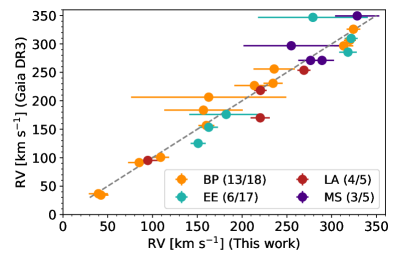
Figure 4: Radial velocity comparison between the values obtained based on COSMOS spectra and Gaia DR3 main source catalogue. Stars corresponding to the BP, EE, LA and MS groups are shown as orange, green, red and purple circles, respectively. The number in parenthesis in the legend is the number of stars having Gaia radial velocities relative to the total number of stars observed in this work.

4.2 Stellar Parameters

Assuming they may slightly vary along the phase, we derive stellar parameters by spectroscopic fitting with the FERRE code (Allende Prieto et al., 2006). FERRE is able to employ different algorithms to minimise the $\chi^{2}$ against a library of stellar spectra (Allende Prieto et al., 2018). Then, by interpolating within the nodes of the grid, the code provides the best stellar model and the most likely effective temperature ($T_{\rm eff}$), surface gravity ($\log g$) and overall metallicity ([Fe/H]).

Both the data and the models were normalised with a running mean filter of 30 pixels. For the purpose of spectroscopic analysis, we masked the Balmer-$\alpha$ line and the regions most affected by telluric lines. Thus, the code does not take into consideration the $\chi^{2}$ from those areas. In Fig. 3 we show a sub-sample of nine spectra and the best fit derived with FERRE. Relevant areas are shaded in yellow while the masked regions are coloured in purple.

In Table 1, we also provide a flag quality by visual inspection of each FERRE fit. In some cases, due to the relatively low quality of the spectra and/or the presence of significant telluric lines, even outside of our masked area, it was not possible to obtain a good fit. For these cases, we set flag=0; for the remainder we set flag=1. Additionally, we performed a complementary analysis deriving metallicities for the entire sample only considering the information contained in the region of the Calcium triple around 8400-8700 Å. We fixed T_eff and $\log g$ from the FERRE analysis, and then calculated $\rm[Fe/H]$_CaT masking everything outside of the considered region. The results are summarised in Table 1, and in most cases are in good agreement with the $\rm[Fe/H]$. However, in some cases, we find a significant deviation between the two determinations, up to 1 dex. The majority of these cases correspond to objects with flag=0, indicating the fit is poor. However, there are 7 cases – BP34, EE10, EE17, EE21, LA42, LA44, and MS04 – where the fit appears reasonable but the metallicities are incompatible. Those objects are quite cool (T_eff$<3800$ K) and the combination of strong molecular bands and the presence of telluric lines could explain the difference. For those objects, we recommend considering the overall metallicity $\rm[Fe/H]$as only a tentative value.

Finally, BP30 and MS04 have been observed twice; in both cases we derived compatible stellar parameters, T_eff, $\log g$, and $\rm[Fe/H]$. The $\rm[Fe/H]$_CaT for these two objects is clearly incorrect and could also be explained as a result of their low-temperature. In fact, the $\rm[Fe/H]$_CaT for BP30 is located at the limit of the grid, indicating the code did not find metallicity information within the CaT.

Table 2: Radial velocities from Gaia DR3. Radial velocity, its error, and S/N of the spectra are the columns radial_velocity, radial_velocity_error and rv_expected_sig_to_noise, respectively.

ID	RVGaia	RV error	S/N
	(km s-1)	(km s-1)
BP22	306.33	2.15	11.6
BP24	325.88	3.13	7.6
BP25	36.64	3.22	8.1
BP26	100.68	1.81	10.7
BP27	296.57	1.89	11.9
BP28	183.59	1.75	6.1
BP32	230.77	3.14	7.4
BP33	34.17	2.99	7.9
BP35	226.80	1.34	11.4
BP36	206.43	3.65	10.8
BP37	255.94	2.21	10.9
BP38	91.36	2.43	8.4
BP39	156.59	4.12	8.0
EE06	309.69	4.95	6.4
EE10	285.53	3.69	4.5
EE16	346.68	2.15	5.5
EE17	176.06	3.9	8.0
EE18	153.48	3.47	4.5
EE52	125.20	4.87	3.8
LA41	218.32	7.91	3.5
LA42	253.76	4.0	3.1
LA43	95.14	7.84	5.7
LA44	170.08	6.88	3.7
MS02	296.82	1.46	5.5
MS03	349.34	2.41	3.9
MS04	271.02	5.15	4.9

The Gaia DR3 parallax, effective temperature, surface gravity, metallicity and spectral type for our targets, when available, are presented in Table 7.

5 6D phase-space information

5.1 Parallaxes and proper motions from Gaia DR3

Even though most of the observed targets have large radial velocities (V${}_{\rm rad}\geq$ 200 km s^-1), it is clear that some targets are most likely foreground contaminants (V${}_{\rm rad}\leq$ 50 km s^-1).

In order to discard those stars and identify potential contaminants with large velocities, parallaxes from Gaia DR3 have been analysed. All the targets have parallaxes between –0.051 mas to 0.036 mas, with the exception of four stars (BP29, BP30, BP31 and BP34) which have parallaxes $>$ 2 mas (see Table 7). These four stars also have proper motions much larger than the other targets, having absolute values greater than 3 mas yr^-1 in each component. In addition, these stars have the lowest radial velocities of all the targets – from –11.70 $\pm$ 6.12 km s^-1 (weighted mean of the two measurements for BP30) to 27.85 $\pm$ 9.65 km s^-1 (BP34) – and the highest values of surface gravity (logg $\approx$ 5.0). We therefore exclude these four dwarf foreground stars for the remaining analysis.

Figure 5 shows the proper motion of our sample, excluding the four contaminants. The grey scale corresponds to a sample of stars up to 10 deg from the LMC and/or SMC center, having G $<$ 17 mag and (G_BP–G_RP) $>$ 1.3 mag (most likely RGB stars). The LMC and SMC stars are clearly seen as overdensities at ($\mu_{\alpha}$, $\mu_{\delta}$) = (1.6, 0.5) mas yr^-1 and (1.1, –1.15) mas yr^-1, respectively. Stars from the MS group have the most similar proper motions to the bulk of the LMC stars, in agreement with previous studies that suggest this northern arc is most likely associated with the LMC disk population (e.g., Cullinane et al., 2022a).

Interestingly, the stars belonging to the BP group have proper motions somewhat different from those of the SMC population. These stars were originally selected as potential debris stars stripped from the SMC, based on their positions in the sky and predictions from simulations of the SMC’s disruption under the LMC potential (Deason et al., 2017). It is also possible that a large fraction of the stars in this group are distant Miras in the Milky Way halo, given their brightness and proper motions close to 0 mas yr^-1. This group of stars is discussed further in Section 5.4.2

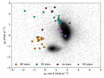
Figure 5: Gaia DR3 proper motions for stars up to 10 deg from the LMC and SMC centers, brighter than G $<$ 17 mag and redder than (BP-RP) $>$ 1.3 mag. Our targets are shown as coloured circles.

After removing the likely foreground contaminants based on their parallaxes, proper motions, and radial velocities, our final sample consists of 41 Mira candidates, with measurements of radial velocities and stellar parameters from COSMOS spectra, and parallaxes and proper motions from Gaia DR3.

In order to study the kinematic behaviour of these stars and their possible origin, a distance estimate is needed. However, at the distance of the LMC, Gaia parallaxes are not a reliable measurement of distance. In the next section, we discuss different approaches to derive the distance of the stars belonging to the MS, LA and EE groups (the closest to the LMC in the sky), making use of well-known Period-Luminosity relations as well as Magellanic RR Lyrae (RRL) stars as anchors for the distance.

5.2 Light curves and periods

In order to confirm the variable nature of our targets and use their periods, if available, to derive distances, we searched for associated light curves in various datasets. From the Gaia DR2 time series, 12 light curves were retrieved. However, only 10 of them have reported frequencies in the Gaia gaiadr2.vari_long_period_variable table. The corresponding periods are reported as P_Gaia in Table 3. Light curves from the All-Sky Automated Survey for Supernovae (ASAS-SN, Jayasinghe et al., 2018) and from the South Catalina survey (SSS, Drake et al., 2017) were also recovered for 23 variables (6 with light curves and periods also reported in Gaia). The two most significant periods from the CRTS survey were used to derive phase-folded light curves, adopting the period that allows us to recover one full pulsation cycle. Figure 6 shows the Gaia $G$ or optical $V$-band CRTS or ASAS-SN light curves for MS01, BP37 and MS05. The time series have very different numbers of epochs; nonetheless, the variability is well recovered.

We adopted the periods from CRTS when available, instead of the Gaia periods, since the former have a larger number of epochs. When only Gaia or ASAS-SN light curves were available, the corresponding period was adopted. The recovered periods range from 65 to 450 days, except for EE13 which has a period of only 1.13 days according to the SSS catalogue. However, the light curve suffers from considerable scatter and the period reported could be due to a 1-day alias. Therefore, for the remainder of the paper, we consider that a reliable period is not available for this star.

In total, periods were recovered for 27 out of 41 Mira candidates. For both the BP and MS group, a high fraction of the Mira candidates have reported periods (12 out of 14 BP stars, and all the MS stars). In the case of the EE and LA stars, light curves were found for only 8 (out of 17) and 2 (out of 5) stars respectively. As a result, only for a subsample of the Mira candidates can distances be derived using any of the Period-Luminosity (PL) relations for LMC stars (see e.g., Soszynski et al., 2007). We proceed to separate this subsample into C-rich and O-rich Miras, and fundamental, first-overtone and long-secondary period pulsators, to apply the corresponding PL relation and derive their distances.

Table 3: Periods for those Mira stars with light curves available in public surveys. Gaia periods are derived from the frequency listed in the gaiadr3.vari_long_period_variable table. Periods are from either CRTS or ASAS-SN catalogues (see main text for details).

ID	PGaia	Plit	Source ID
	(d)	(d)
BP22	366.16	335.12	SSS J101029.1-314452
BP23	122.99
BP24	103.14	106.53	SSS J111716.7-362011
BP25	121.03	124.26	SSS J102952.7-332925
BP26	407.05	392.42	SSS J103936.2-370853
BP27	116.71	114.01	SSS J102457.2-312547
BP32		103.73	SSS J093018.0-210453
BP33	389.43	413.14	SSS J100707.0-192403
BP35	110.49	111.22	SSS J112538.0-285553
BP36	144.37	145.12	SSS J115027.0-432228
BP37		128.00	ASAS_SN-V J120352.76-403726.3
BP38		64.92	SSS J113754.5-335839
BP39	120.80	119.42	SSS J114558.0-271337
EE06	134.29	132.00	ASAS_SN-V J084919.03-704150.2
EE07	181.09	180.52	SSS J074344.4-691805
EE10	181.55
EE11	56.62
EE12	313.12
EE13		1.13	SSS J072216.5-634214
EE14	286.41	285.06	SSS J071218.6-633809
EE16	225.63	225.00	ASAS_SN-V J065604.73-635441.5
EE17	473.49
EE19	301.47	325.49	SSS J064152.5-623852
LA40	423.36
LA41		65.88	ASAS_SN-V J084251.71-833038.3
LA43	132.11
LA44	156.63
MS01	398.43
MS02	36.16	161.06	SSS J071821.2-551943
MS03	158.75	156.39	SSS J064806.4-530033
MS04	139.56	146.65	ASAS_SN-V J054138.80-542008.6
MS05	215.95	219.39	SSS J062806.1-531105

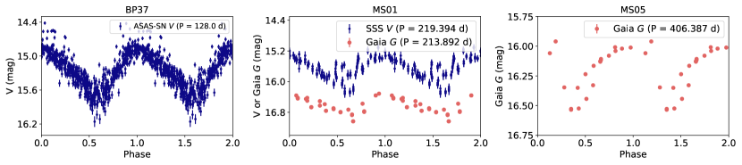
Figure 6: Gaia $G$ and optical $V$-band light curves for three Mira stars in our sample. From left to right: Gaia $G$-band light curve and period for MS01; ASAS-SN optical $V$-band light curve and period for BP37; periods and light curves from the Gaia and CRTS surveys for MS05.

5.3 Photometric chemical-types

Among long-period variables (LPVs), different masses and types of stars can be found. Depending on the evolutionary state (RGB or AGB star), mass regime and surface chemistry (C/O-rich), these stars follow different $K_{\rm S}$ and Gaia $G$ PL relations (Lebzelter et al., 2019). The K_S PL diagram for LPVs in the LMC shows different relations for C-rich and O-rich red giants, as well as for fundamental and first overtone pulsating Miras, semi-regular variables and long-secondary period variables (see e.g., Soszynski et al., 2007). Therefore, identifying the sub-type of each of the targets in our sample is necessary in order to derive distances for those stars with measured periods (see Section 5.2).

A powerful diagram to separate the different sub-types of pulsating giant stars is the (W_RP - W_J,Ks) versus K_S diagram presented by Lebzelter et al. (2018). Combining optical Gaia $G$, G_BP, G_RP magnitudes and near-IR 2MASS $J$ and K_S magnitudes, the Wesenheit functions W_RP and W_J,Ks allow us to use reddening-free magnitudes. Lebzelter et al. (2018) defined a boundary to separate C-rich from O-rich LPVs in the LMC based on the (J-K_S) colours, with C-rich stars being those with redder near-IR colour (i.e., having W_RP - W_J,Ks $\gtrsim$ 0.8 mag). Among the O-rich stars, using population synthesis models, Lebzelter et al. (2018, 2019) define different boundaries to separate low, intermediate and high-mass pulsating AGB stars, while the faintest O-rich stars (K${}_{\rm S}\geq$ 12 mag) are mostly early AGB and RGB stars from the tip of the RGB in the LMC.

We cross-match our targets with the Gaia DR3 and 2MASS catalogues, using a search radius of 1.0 arcsec. The Wesenheit functions were calculated following the original definition in Lebzelter et al. (2018), as follows:

$$W_{\rm BP,RP} =G_{\rm RP}-1.3\left(G_{\rm BP}-G_{\rm RP}\right)$$ (1)

$$W_{\rm J,Ks} =K_{\rm S}-0.686\left(J-K_{\rm S}\right)$$ (2)

Figure 7 shows the location of our target stars (from the three groups close to the LMC: MS, EE and LA) in the (W_RP - W_J,Ks), K_S diagram. The boundaries from Lebzelter et al. (2019) are shown as dashed lines, while the corresponding sub-types are shown as green (O-rich RGB and faint, early AGB stars), blue (O-rich low-mass AGB stars), cyan (O-rich intermediate-mass AGB stars), red (C-rich) and yellow (extreme C-rich) circles. None of our targets have colours and magnitudes in the location of red supergiants (RSG) or O-rich massive AGB stars. We find that most (22 out of 27) of our targets are O-rich stars, while five are C-rich including one extreme C-rich star (though note that two stars have colours on the boundary between C and O-rich groups). Among the O-rich stars, 9 have colours and magnitudes consistent with RGB stars or faint, early AGB (green circles); one star (cyan circle) has properties consistent with being an intermediate-mass (initial stellar masses, M${}_{i}\gtrsim$ $\sim$2.0 to $\sim$3.2 M_⊙) AGB star; and the remainder (12 out of 27) are consistent with being O-rich low-mass (M${}_{i}\sim$ 0.9 to $\sim$1.4 M_⊙) early AGB or thermal-pulsating AGB stars.

Half of the stars (14 out of 27) in Figure 7 have periods available, and distances can thus be estimated using PL relations.

The targets from the BP group were not included in this diagram since the boundaries from Lebzelter et al. (2018) are defined for the LMC distance modulus. The Mira stars in the BP group are far from the Clouds and their distances could be quite different from the LMC. We discuss this particular group in the next Section.

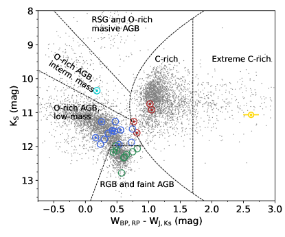
Figure 7: W${}_{\rm BP,RP}-$ W${}_{\rm J,K_{\rm S}}$ versus K_S diagram for LPV stars around the LMC (grey dots) as well as the Miras-like stars belonging to the EE, MS and LA groups. The boundary lines that separate C-rich from O-rich stars, as well as the different mass regimes, are marked as dashed lines (taken from Lebzelter et al. 2019). Our sample is mainly comprised of O-rich low-mass AGB stars. Those stars with periods available in the literature are denoted with a coloured dot inside the marker.

5.4 Distance determination

5.4.1 Stars around the Large Magellanic Cloud

Following the classification into sub-types from Lebzelter et al. (2019), we divided the Mira candidate stars around the LMC from Gaia into C-rich stars, O-rich stars and RGB or faint AGB stars (with magnitudes consistent with the tip of the LMC’s AGB). The top panel of Figure 8 shows the Wesenheit W_J,Ks - period diagram for those stars classified as extreme C-rich (yellow points) and C-rich (red points); the middle panel shows the O-rich low (blue) and intermediate-mass (cyan) AGB stars, and the bottom panel includes only the stars consistent with being RGB or faint AGB stars (green points). The larger coloured points correspond to our targets (one extreme C-rich, four C-rich, six O-rich low-mass, one O-rich intermediate-mass and two RGB/faint AGB stars), while the smaller coloured dots are the LPV stars from the Gaia DR2 catalogue of LPV candidates in the different subgroups shown in Fig. 7.

In each panel, the best-fit PL relations from Soszynski et al. (2007), based on the Optical Gravitational Lensing Experiment (OGLE) observations, are shown for first-overtone pulsators (dashed lines), fundamental mode pulsators (solid lines) and long-secondary period variables (dotted lines), for both O-rich (grey) and C-rich (black) red giant variables. The coloured dots in each panel correspond to LPVs variables in the LMC, selected following the same selection criteria as in Lebzelter et al. (2018), and cross-matched with the 2MASS photometry.

As already noted by Lebzelter et al. (2019), there is significant scatter and deviations from the best PL relations in all pulsation modes, reflecting inaccurate 2MASS mean magnitudes (one single measurement over the pulsation period) as well as underestimated periods, shifting the distribution of LMC LPVs towards shorter periods. This effect is clearly seen in the case of the RGB and faint AGB stars (bottom panel in Figure 8), which are found mostly pulsating in the long-secondary period (the stars with the longest periods in the sample), and which are systematically offset from the PL relation. In fact, all the stars with the longest ($>$300 days) periods in our sample – i.e., EE19, MS01 (C-rich RGB and faint AGB stars), LA40 (low-mass AGB star), and EE17 (intermediate-mass AGB star) – are systematically offset from the PL relation of the most likely pulsation mode. Therefore, these LPVs cannot be used as precise distance estimators unless the time-series photometry is sufficient to recover reliable period estimates.

In the case of the extreme C-rich stars (yellow points, middle panel of Figure 8), these are expected to be pulsating in the fundamental mode. Nonetheless, there is considerable scatter in their magnitudes with respect to the corresponding PL sequence derived by Soszynski et al. (2007). This scatter can be due to stars that are highly reddened and/or stars producing high-opacity dust grains.

If all our targets were of the Mira variability class, they should be pulsating in the fundamental mode. Nonetheless, given the selection made to recover them, we cannot rule out that some of our targets are instead semi-regular variables which could be pulsating in the fundamental or first-overtone pulsation modes. In fact, as Fig. 8 shows, C-rich stars with large periods (P $>300$ d) tend to be in the locus for those stars in the long-secondary period group (green dots), while stars with short periods ($P<$ 100 d) preferentially pulsate in the first-overtone mode. Assuming that each of our targets is pulsating in the pulsation mode corresponding to the closest relation in Fig. 8, we derived their distance moduli using the Wesenheit W_J,Ks PL relations from Soszynski et al. (2007). To obtain the individual distances, a distance modulus of 18.477 $\pm$ 0.004 (statistical) $\pm$ 0.026 (systematic) mag (Pietrzyński et al., 2019) for the LMC was adopted.

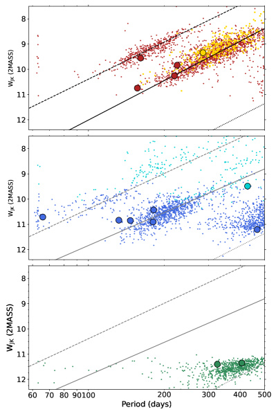
Figure 8: Wesenheit index W_J,Ks – PL diagrams for LPVs in the LMC, colour-coded according to their classification in the Gaia-2MASS diagram (see Fig. 7). In the top panel, C-rich (red) and extreme C-rich (yellow) stars are shown, along with the five Mira variables found to be consistent with this classification. The middle panel shows those stars classified as O-rich AGB stars of low (blue) and intermediate (cyan) mass, while the bottom panel presents the RGB and faint AGB stars (green). The best-fit PL relations for the first overtone, fundamental mode and long-secondary period sequences are shown as dashed, solid and dotted grey/black lines for O/C-rich stars, according to Soszynski et al. (2007).

In the case that all our targets are Miras, pulsating in the fundamental mode, the distances would be $\sim$2 times shorter ($\sim$ 4 times larger) for those stars considered to be pulsating in the first-overtone (long-secondary period). This scenario is unlikely, however, as our targets are close to the LMC in the sky and it is more plausible to find distant ($\sim$ 50 kpc) long-period (Mira-like) variables around the LMC periphery than finding Milky Way halo Miras at less than 30 kpc close to the LMC, or Mira candidates at distances more than 200 kpc.

In order to confirm the order of magnitude of the distances obtained with the limited information we have about our targets’ pulsation mode, Fig. 9 shows the distances obtained for our targets on top of the distribution of the Magellanic RRL stars. The top and middle panels show the distance of our targets based on the PL relations and the median distance of the closest 5 RRL to each of our targets. The bottom panel shows the standard deviation in the RRL distance. The figure shows that RRLs trace substructures around our targets from 42 to 52 kpc, with a mean distance of 45 kpc (with median errors bars of less than 5 kpc). While our targets are at distances from 36 kpc to 59 kpc, their mean distance is $\sim$ 46 kpc, as in the case of RRLs.

Table 4 presents the different sub-types for our targets based on Figure 7 (i.e., C-rich or low-mass, intermediate-mass and RGB O-rich stars), their pulsation mode based on Figure 8, and their associated distance. For those stars at the boundary of being O-rich/C-rich (MS03 and MS05), both possible distances are reported.

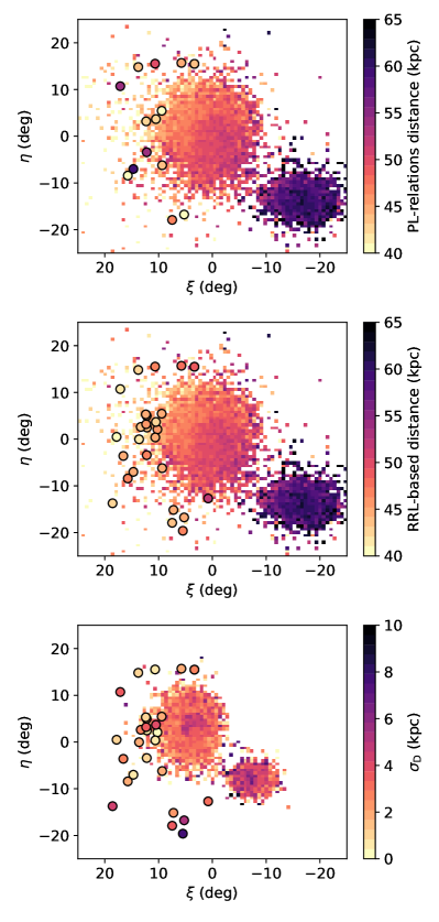
Figure 9: Heliocentric distances for different stellar tracers around the Clouds. The 2D histogram shows the mean distance (top and middle panels) of RRL stars around the Clouds and its standard deviation (bottom panel). The top panel shows as coloured circles those targets with available distances, based on PL relations. The middle and bottom panels respectively show the mean heliocentric distances and standard deviation for RRL stars around the on-sky position of our targets.

Table 4: Heliocentric distances from PL relations. The sub-types (C- or O-rich, low-mass, intermediate-mass or RGB) for those stars with available periods is presented. The pulsation mode (FM: fundamental mode, FO: first-overtone, LSP: long-secondary period) adopted to derive distances is also included. Errors on the distances are from the propagation of uncertainties on the PL relation coefficients, LMC distance modulus and 2MASS magnitudes.

ID	Sub-type	Pulsation mode	Distance
			(kpc)
EE06	O-rich (low)	FM	39.8 $\pm$ 1.2
EE07	O-rich (low)	FM	53.9 $\pm$ 1.7
EE10	O-rich (low)	FM	43.5 $\pm$ 1.3
EE14	Extreme C-rich	FM	43.0 $\pm$ 1.9
EE16	C-rich	FM	42.3 $\pm$ 1.7
EE17	O-rich (mid)	FM	59.3 $\pm$ 2.3
EE19	O-rich (RGB)	LSP	36.7 $\pm$ 1.5
LA40	O-rich (low)	LSP	47.0 $\pm$ 2.0
LA41	O-rich (low)	FO	38.9 $\pm$ 1.0
MS01	O-rich (RGB)	LSP	44.2 $\pm$ 1.8
MS02	C-rich	FO	53.8 $\pm$ 1.6
MS03	C-rich/O-rich (low)	FM	44.1 $\pm$ 1.6/44.2 $\pm$ 1.3
MS04	O-rich (low)	FM	43.8 $\pm$ 1.3
MS05	C-rich/O-rich (low)	FM	50.0 $\pm$ 2.1/47.3 $\pm$ 1.6

5.4.2 Stars above the Galactic plane (BP group)

Among our targets, after discarding the four foreground stars with large parallaxes, there are 14 Mira candidates located above the Galactic plane. Given their position on the sky, these stars could be unrelated to the Clouds, and distance determination is thus more uncertain.

Most of these stars do, however, have periods available (see Table 3) which can in principle be used to derive distances. Figure 10 shows the position of these stars in the period - W_J,Ks diagram, as well as the best PL sequences for O-rich LPVs around the LMC. In contrast with the stars discussed in section 5.4.1, these stars can be easily at less than 30 kpc (i.e., be bright stars pulsating in the fundamental mode) and no assumptions can be made regarding their pulsation modes. We therefore report the two most likely distances (based on how close each star is to the different PL sequences) in Table 5.

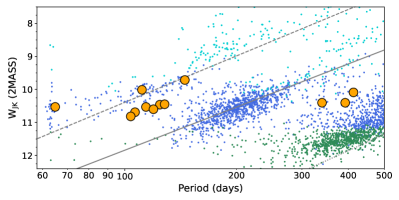
Figure 10: Period - magnitude diagram for the stars located above the Galactic plane. The PL sequences for first-overtone (dashed line), fundamental mode (solid line) and LSP (dotted line) LPV stars in the LMC are included. The distribution of LPV stars in the LMC are shown as blue, cyan and green symbols as in Figure 8.

Table 5: Heliocentric distance estimates for the BP stars. The distances for two possible pulsation modes are reported. Errors on the distances are obtained by propagating the uncertainties as in Table 4.

ID	Pulsation	Distance	Pulsation	Distance
	mode	(kpc)	mode	(kpc)
BP22	FM	74.0 $\pm$ 2.7	LSP	24.2 $\pm$ 0.9
BP24	FO	60.4 $\pm$ 1.5	FM	30.8 $\pm$ 0.9
BP25	FO	62.8 $\pm$ 1.6	FM	31.7 $\pm$ 0.9
BP26	FM	83.8 $\pm$ 3.2	LSP	27.6 $\pm$ 1.1
BP27	FO	59.8 $\pm$ 1.4	FM	30.4 $\pm$ 0.8
BP32	FO	62.5 $\pm$ 1.5	FM	32.0 $\pm$ 0.9
BP33	FM	75.9 $\pm$ 2.9	LSP	25.1 $\pm$ 1.0
BP35	FO	46.0 $\pm$ 1.1	FM	23.4 $\pm$ 0.7
BP36	FO	51.4 $\pm$ 1.3	FM	25.7 $\pm$ 0.8
BP37	FO	64.2 $\pm$ 1.5	FM	32.4 $\pm$ 0.9
BP38	FO	35.3 $\pm$ 0.9	FM	18.6 $\pm$ 0.6
BP39	FO	64.5 $\pm$ 1.6	FM	32.7 $\pm$ 1.0

Given the uncertain distances for these stars, and their proper motions centered on $(\mu_{\alpha},\mu_{\delta}$) = (0, 0) mas yr^-1, we cannot rule out the possibility of them being distant ($\sim$ 30 kpc) Galactic Mira-like stars, rather than being associated with the LMC or SMC. This group of stars is located close to the predicted area of the sky where tidally-stripped LMC RRL stars have been reported by Petersen et al. (2022). However, based on the mock observations presented in Petersen et al., LMC debris is expected to have much larger line-of-sight velocities than that measured for the BP stars (V${}_{\rm los}>$ 300 km s^-1). Further investigation to understand the origin of the BP stars (as likely distant Galactic Mira-like stars) is needed, however it is beyond the scope of this work. Accordingly, for the remainder of this paper, we will focus on the Mira-candidates in the vicinity of the Clouds.

6 Outer periphery of the LMC

Figure 11 shows the phase-space information available for the targets in the three different groups of stars in the Magellanic periphery. The on-sky position as well as radial velocities, proper motions and distances, are shown. The angle $\phi$ is used as a position angle, going from 0 to 180° anticlockwise from North toward South. In the bottom row, the mean distance of the closest RRL is presented as a grey symbol. In this figure, it is possible to recognise trends and isolate potential outliers for each group.

In the case of the MS stars (left panels), the target at the largest on-sky distance with respect to the LMC center (MS02, $\phi$ = 60°) has a rather smaller radial velocity and potentially deviating distance compared to the rest of the stars in the group. As a comparison, the left panels include the measurements presented by Cullinane et al. (2022a) for different fields along the northern arm (violet crosses). It is clear that our targets trace the same trends in radial velocity and proper motions as in Cullinane et al. (2022a), with MS02 most likely being an outlier. The trend in distances, being those stars at large $\phi$ slightly more distant than those close to the LMC center, can be explained considering the inclination and orientation of the line of nodes of the LMC plane, as already discussed in Cullinane et al. (2022a).

For the LA stars (right panels), there seems to be one outlier based on its rather small radial velocity and proper motions (LA43, $\phi$ = 165°). LA 44, at $\phi$ = 176°, also has a deviating proper motion compared to the rest of the stars in the group. We therefore consider both as potential contaminants.

In the case of EE stars, most of the stars have large ($>$ 300 km s^-1) velocities, except for three stars: EE17, EE18 and EE22. These stars are located at the largest on-sky distances from the LMC center. Their proper motions, particularly $\mu_{\alpha^{\ast}}$, also deviate from the other stars in the group. We decided to flag them as potential outliers, although it could be that these stars are instead tracing a different structure, as they all have very similar, relatively large velocities ($>$ 150 km s^-1).

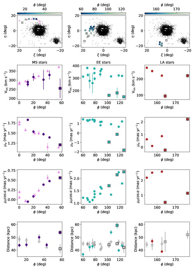
Figure 11: Phase-space properties for our targets. The left, middle and right panels correspond to stars in the MS, EE and LA groups. The top panels show the on-sky distribution of the Mira candidates selected by Deason et al. (2017). In the left panels, the violet triangles are measurements from Cullinane et al. (2022a) for different fields along the LMC northern arm. Distances derived based on PL relations are shown as coloured circles, while those corresponding to the mean distance of the closest RRL stars are shown as grey open circles. Possible kinematic outliers for each group are denoted with open square outlines in each panel.

6.1 3D motions

With 6D phase-space information in hand, the 3D motion for each star in the LMC reference frame can be calculated. In particular, the cylindrical velocities (V_R, V_ϕ and V_Z) can be used to assess the origin (e.g., disturbed LMC disk stars) of our targets. Based on the van der Marel & Cioni (2001); van der Marel et al. (2002) formalism, the radial motion V_R, azimuthal motion V_ϕ and the velocity perpendicular to the disk plane V_Z, can be estimated as

$$V_{R}=\left(x^{\prime}v_{x}^{\prime}+y^{\prime}v_{y}^{\prime}\right)/R\text{,}$$ (3)

$$V_{\phi}=\left(y^{\prime}v_{x}^{\prime}-x^{\prime}v_{y}^{\prime}\right)/R\text{,}$$

$$V_{Z}=v_{z}^{\prime}\textbf{.}$$

$R$ is the in-plane radial distance of a tracer to the LMC center, while (v${}_{x}^{\prime}$, v${}_{y}^{\prime}$, v${}_{z}^{\prime}$) are the Cartesian velocities in the plane of the LMC disk, after subtracting the LMC systemic motion. To derive these Cartesian velocities, the formalism derived by van der Marel & Cioni (2001); van der Marel et al. (2002) was followed. The LMC center-of-motion (COM) was fixed at ($\alpha_{0}$, $\delta_{0}$) = (79$\aas@@fstack{\circ}$88, –69$\aas@@fstack{\circ}$59) (van der Marel & Kallivayalil, 2014), while the line-of-sight velocity and the proper motions of the COM used were V_los = 261.1 km s^-1, and ($\mu_{\alpha}\cos{\delta}$, $\mu_{\delta}$) = (1.895, 0.287) mas yr^-1, from van der Marel & Kallivayalil (2014). The adopted LMC heliocentric distance was $D_{\rm H}$ = 49.5 kpc (Pietrzyński et al., 2019). For the LMC disk geometry, the values reported by Choi et al. (2018) were used, following the discussion in Cullinane et al. (2022a): i.e., $i$ = 25$\aas@@fstack{\circ}$86 and $\theta$ = 239$\aas@@fstack{\circ}$23 respectively.

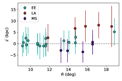
Figure 12: In-plane radial distance $R$ versus vertical distance z${}^{{}^{\prime}}$ for the stars in the vicinity of the LMC. Beyond $\sim$15°, the stars are far from the LMC disk plane.

We adopted the distances of the closest RRL stars in the sky as a first rough estimate of the distance of each Mira candidate, even for those without periods available in the literature. As shown in Fig. 9, for those stars with available periods, the distance derived using PL-relations for long-period variables in the LMC and those obtained based on the closest RRL stars are compatible. To test the influence of the distance determination used, we also computed the cylindrical velocities assuming that all our targets are on the LMC disk plane (z’ = 0 kpc), and therefore their on-plane distance is derived as

$$D_{\rm disk}=\frac{D_{0}\cos{i}}{\cos{i}\cos{\rho}-\sin{i}\sin{\rho}\sin{(\phi-\theta)}},$$ (4)

where $(\rho,\phi)$ are the on-sky distance and position angle of our targets respectively. The cylindrical velocities obtained this way are, for most of the stars, compatible within the errors with those values derived adopting the RRL-based distance. However, for the stars at a large projected radius $R$, the vertical position $z^{{}^{\prime}}$ could significantly deviate from the disk plane. Figure 12 shows the in-plane projected radius $R$ of each star and the corresponding vertical position z${}^{{}^{\prime}}$, estimated based on the RRL-based distance, which is positive for stars above the LMC disk (in the direction towards the observer). Stars located at $R>$ 14° are located more than 5 kpc away from the LMC disk, in agreement with the results for red-clump stars presented in Cullinane et al. (2022b). Therefore, we adopted the individual distances for each star instead of assuming that all of them are located in the LMC disk plane. The gnomonic-projected coordinates ($\eta$, $\xi$) and 3D velocities are presented in Table 6, including the corresponding errors derived from the propagation of the uncertainties in the measured proper motions, radial velocities and distances.

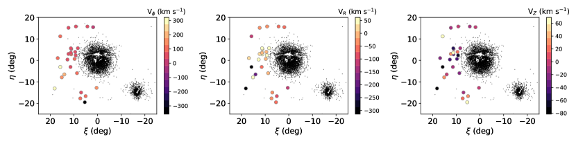
Figure 13: The azimuthal velocity (V_ϕ), radial velocity (V_R), and vertical velocity (V_Z) for our targets. The dashed circle marks 9° from the LMC center. The black points are the Mira candidates from Deason et al. (2017)

Table 6: 3D cylindrical velocities in the LMC coordinate system.

ID	$\xi$	$\eta$	Vϕ	VR	VZ
	(deg)	(deg)	(km s-1)	(km s-1)	(km s-1)
EE06	15.2	–7.9	135.9 $\pm$ 5.5	43.9 $\pm$ 6.0	33.8 $\pm$ 6.6
EE07	11.5	–3.0	33.3 $\pm$ 7.8	–48.5 $\pm$ 7.9	–13.1 $\pm$ 9.4
EE08	12.7	0.4	48.1 $\pm$ 8.2	37.1 $\pm$ 8.2	–39.9 $\pm$ 7.9
EE09	9.3	2.4	38.4 $\pm$ 8.2	39.6 $\pm$ 8.7	–60.8 $\pm$ 7.9
EE10	8.7	–5.9	85.2 $\pm$ 6.8	–5.3 $\pm$ 7.8	–26.8 $\pm$ 9.0
EE11	9.7	0.7	81.5 $\pm$ 11.9	0.4 $\pm$ 8.7	–38.6 $\pm$ 18.9
EE12	11.2	2.8	86.5 $\pm$ 8.2	44.1 $\pm$ 8.1	–29.2 $\pm$ 7.9
EE13	12.3	3.0	68.2 $\pm$ 8.8	23.6 $\pm$ 7.5	36.5 $\pm$ 12.1
EE14	11.3	3.5	55.0 $\pm$ 39.3	–3.8 $\pm$ 21.7	69.0 $\pm$ 70.2
EE15	11.2	5.3	66.9 $\pm$ 8.1	11.5 $\pm$ 6.5	–7.9 $\pm$ 12.2
EE16	9.5	4.0	72.7 $\pm$ 27.6	–12.4 $\pm$ 12.2	22.6 $\pm$ 54.1
EE17	14.1	–6.5	222.5 $\pm$ 14.7	–189.2 $\pm$ 21.5	4.2 $\pm$ 32.7
EE18	15.8	–3.1	321.5 $\pm$ 6.8	–305.5 $\pm$ 6.4	–78.6 $\pm$ 8.9
EE19	8.4	5.7	78.6 $\pm$ 7.8	61.6 $\pm$ 7.5	–12.9 $\pm$ 7.9
EE20	16.9	1.1	82.6 $\pm$ 7.9	10.2 $\pm$ 7.0	–23.4 $\pm$ 9.2
EE21	11.3	5.6	39.4 $\pm$ 7.7	43.5 $\pm$ 6.8	–49.6 $\pm$ 10.1
EE22	18.2	–13.0	283.1 $\pm$ 5.4	–314.1 $\pm$ 6.8	–81.4 $\pm$ 7.1
LA40	7.3	–17.7	81.9 $\pm$ 5.7	–41.2 $\pm$ 6.4	20.5 $\pm$ 6.9
LA41	5.1	–16.6	122.1 $\pm$ 6.5	–73.0 $\pm$ 6.6	34.7 $\pm$ 6.8
LA42	7.0	–14.9	43.8 $\pm$ 6.7	–40.2 $\pm$ 6.7	–9.1 $\pm$ 6.9
LA43	5.4	–19.5	–357.4 $\pm$ 6.5	–52.0 $\pm$ 8.0	64.1 $\pm$ 9.9
LA44	0.4	–12.8	133.4 $\pm$ 7.8	–102.6 $\pm$ 8.0	–1.5 $\pm$ 9.9
MS01	4.3	15.8	51.9 $\pm$ 15.8	–48.5 $\pm$ 15.6	–16.1 $\pm$ 51.1
MS02	15.8	11.2	96.5 $\pm$ 22.1	–99.8 $\pm$ 18.1	64.5 $\pm$ 45.8
MS03	12.3	15.2	67.1 $\pm$ 9.7	–40.8 $\pm$ 9.6	–6.6 $\pm$ 22.1
MS04	1.9	15.5	–2.9 $\pm$ 6.0	–50.1 $\pm$ 6.0	2.3 $\pm$ 11.1
MS05	9.2	15.8	47.7 $\pm$ 9.2	–25.4 $\pm$ 9.0	–0.4 $\pm$ 19.5

Fig. 13 shows the $V_{\phi}$ (left panel), V_R (middle panel) and V_Z (right panel) for all our targets. It is evident that the largest variations in velocity are found at the largest angular distances from the LMC (i.e., outer EE and LA stars). The azimuthal velocity is consistent with V_ϕ $\sim$ 70 km s^-1, which is the constant value reached by the LMC rotation curve (see e.g., Wan et al., 2020; Gaia Collaboration et al., 2021; Cullinane et al., 2022b) for most of the stars, particularly those in the northern arm. A few stars have excessively large azimuthal velocities, of the order of 300 km s^-1, corresponding to those with line-of-sight velocities $<$ 200 km s^-1, while one of the LA stars has a counter-rotating motion. These deviating azimuthal velocities could be due to perturbations in the outer LMC.

The in-plane radial velocity, V_R, mildly deviates from a disk in equilibrium for several stars. In the case of those stars in the northern arm (MS), an inward motion of $\sim-$46 km s^-1 is found, consistent with the measurements of Cheng et al. (2022) and Cullinane et al. (2022a). For the outer EE stars and LA stars, however, V_R reaches much larger values, up to $-$250 km s^-1, reinforcing the idea of these being perturbed LMC disk material. Large inward velocities were also reported by Cheng et al. (2022) towards the south of the LMC.

The possible outlier in the MS group, MS02 (see Fig. 11), is located slightly off from the track of the northern arc, inside the so-called "North-East Structure" (NES, Gatto et al., 2022). Based on proper motions from Gaia, the NES was found to have in-plane velocities V_R, V_ϕ similar to the stars in the northern arm, suggesting a possible common origin. We found, however, that the out-of-plane velocity V_Z strongly deviates from the values for the rest of MS stars, which are consistent with a disk in equilibrium.

The out-of-plane velocities, V_Z, of other stars largely deviate from a disk in equilibrium, reaching up to $-$80 km s^-1 (EE22). Similar to the results in Cullinane et al. (2022a), the out-of-plane velocities for the stars in the northern arm appear to be out of equilibrium. However, owing to the large errors in radial velocities for the MS stars, the error on V_Z does not allow us to confirm this behaviour. As those stars in the N1 and N2 fields of Cheng et al. (2022), the radial and rotational motion of these stars is compatible with a disk origin. Cullinane et al. (2022a) found consistent velocities in the seven fields tracing the northern arm (see dashed blue circles in Fig. 1), finding that the stars in them have a mean while V_ϕ of the order of $\sim$70 km s^-1, consistent with the rotation curve of the LMC (see e.g., Wan et al., 2020; Gaia Collaboration et al., 2021). On contrast, V_R and V_Z are deviated from zero, expected for a disk in equilibrium. The five MS stars have an inward radial motion of $\sim$40 km s^-1, similar to the value derived in Cullinane et al. (2022a). The in-plane vertical motion shows larger deviations, reaching up to 135 km s^-1. Discarding this measurement, the other four stars have a mean V_Z of 32 km s^-1. Similar values are found in the APOGEE fields analyzed by Cheng et al. (2022). We can therefore conclude that all MS Mira candidates are consistent with LMC perturbed disk material.

The 3D velocities of the EE stars in the northern-east area ($\eta$, $\xi>$ 0°) are consistent with a perturbed disk, having a median azimuthal velocity of $V_{\phi}\sim$ 65 km s^-1, in-plane radial velocities V_R going from almost zero up to $\sim$60 km s^-1, and negative out-of-plane velocities. These relatively large in-plane radial and out-of-plane velocities are contrary to the findings of Cullinane et al. (2022b), based on the aggregate motion of red clump stars in three fields at the north-east of the LMC, which were found to be consistent with a disk in equilibrium. This apparent disagreement can potentially be due to the larger angular separations from the LMC center traced by the EE stars (from to 16° up to $\sim$21°) compared to the fields in Cullinane et al. (2022a) (see Fig. 1).

For the EE stars in the southern-east region, the azimuthal and in-plane radial velocities are exceedingly large, reaching out to $V_{\phi}\gtrsim$ 300 km s^-1 and V${}_{R}\sim$ –300 km s^-1. These large 3D velocities can be explained based on the different line-of-sight velocities and proper motions of these stars, see the middle panels in Figure 11. The three potential outliers have relatively large line-of-sight velocities ($>$ 150 km s^-1) but are considerably lower than the rest of the stars in the EE group. The proper motions in the R.A. direction also strongly deviate from the values for stars in the area of sky which have smaller angular distances. We therefore cannot rule out the possibility of these stars being extremely disturbed LMC disk stars. The other EE stars in the south-east have very different 3D velocities, reflecting the fact that towards the south, the LMC disk is kinematically disturbed (Cheng et al., 2022; Cullinane et al., 2022b).

In the south, stars from the LA group also show deviations from a disk in equilibrium. LA43 and LA44, previously identified as potential outliers based on their line-of-sight velocities and/or proper motions, have extreme $V_{\phi}$ velocities. LA43 is found to be counter-rotating with respect to the LMC disk, while moving inwards the LMC, with V${}_{R}\sim$ – 50 km s^-1. Stars from the LA group are located towards the same direction in which Olsen et al. (2011) found potential SMC debris, with apparent counter-rotating line-of-sight velocities. The CaT metallicity derived for LA43 is [Fe/H] $=-$1.42, in fair agreement with CaT metallicities for SMC stars. There are no spectroscopic studies in the literature with observations at angular distances $>$ 18°in the southern area around the LMC, and therefore we cannot compare this result with previous observations.

The rest of the stars in the LA group are placed close to the southern arm-like feature reported in Belokurov & Erkal (2019). LA42 has 3D kinematics consistent with a disk in equilibrium, although the vertical distance is $\sim$8 kpc above the LMC disk plane. These results are in very good agreement with the measurements for field 26 from Cullinane et al. (2022b), which is very close to LA42 on the sky. LA40 and LA41 have negative inward velocities and positive out-of-plane velocities, consistent with perturbed disk material, in contrast to the relatively unperturbed inner southern LMC disk reported in Cullinane et al. (2022b), and in better agreement with the results from Cheng et al. (2022) for the southern periphery of the LMC.

7 Comparison with simulations

7.1 Simulation setup

In order to explore how this dataset constrains the LMC-SMC interaction history, we produced a suite of numerical simulations. This suite is based on the simulations in Belokurov & Erkal (2019); Cullinane et al. (2022a, b). In particular, we model the interaction of the LMC-SMC in the presence of the Milky Way. We model the LMC with a Hernquist (Hernquist, 1990) dark matter halo and an exponential stellar disk. For the Hernquist profile, we use a mass of $1.5\times 10^{11}M_{\odot}$, motivated by the results of Erkal et al. (2019), and a scale radius of 20 kpc. This scale radius is chosen to match the circular velocity of the LMC measured at 8.7 kpc (van der Marel & Kallivayalil, 2014). For the exponential disk, we use a mass of $2\times 10{9}M_{\odot}$, a scale radius of 1.5 kpc, and a scale height of 0.4 kpc. As in Cullinane et al. (2022a, b), we simulate the exponential disk with tracer particles and model the gravitational potential of the LMC with a particle sourcing the combined Hernquist and exponential disk potentials. We initialize the disk with $10^{7}$ particles using agama (Vasiliev, 2019) but only simulate the $\sim$2500000particles which have apocenters larger than 7 kpc since our dataset is focused on the outer LMC.

The potential of the SMC is modelled as a logarithmic potential (i.e. with a flat rotation curve) within 2.9 kpc with a circular velocity of 60 km/s, based on the observations in (Stanimirović et al., 2004). Beyond 2.9 kpc, the SMC is modelled as a Hernquist profile with a mass of $2.5\times 10^{9}M_{\odot}$ and a scale radius of 0.043 kpc. This scale radius is chosen to match the observed circular velocity at 2.9 kpc. We note that we model the inner regions of the SMC as a logarithmic potential to avoid any unphysically large perturbations during its close encounter with the LMC disk. During the simulation, the SMC is modelled as a particle sourcing this potential.

The Milky Way is modelled as a 3-component system with an NFW dark matter halo, a Hernquist bulge, and a Miyammoto-Nagai disk based on the mwpotential2014 model in Bovy (2015). The NFW halo has a mass of $8\times 10^{11}M_{\odot}$, a scale radius of 16 kpc, and a concentration of 15.3. The Miyamoto-Nagai disk has a mass of $6.8\times 10^{10}M_{\odot}$, a scale radius of 3 kpc, and a scale height of 0.28 kpc. The Hernquist bulge has a mass of $5\times 10^{9}M_{\odot}$ and a scale radius of 0.5 kpc. During the simulation, the Milky Way is allowed to move in response to the LMC and SMC. This is done by treating the Milky Way as a single particle which sources its three-component potential.

During each simulation, the LMC and SMC are initialized given their present-day position and velocity with the Milky Way placed at the origin. The Milky Way, LMC, and SMC are rewound for 2 Gyr. At this time, the tracer particles representing the LMC disk are injected and the simulation is evolved to the present day. Since the tracer particles have a range of orbital timescales with respect to the LMC, the tracer particles are individually evolved to the present day for computational efficiency.

Our suite consists of four sets of 100 simulations of the LMC-SMC-Milky Way encounter which differ on the present-day LMC and SMC positions and velocities. For the first set, we sampled the LMC and SMC position and velocity based on observations of their proper motions, radial velocities, and distances from Kallivayalil et al. (2013); van der Marel et al. (2002); Harris & Zaritsky (2006); Pietrzyński et al. (2019); Graczyk et al. (2014) respectively. We then simulated 100 realizations of the LMC and SMC’s present-day positions and velocities and simulated each of these. Interestingly, in 51 of these realizations, the SMC has a negligible effect on the LMC disk since it has no close crossings with the LMC disk in the past, and thus the majority of the simulations in this suite were essentially unperturbed. For the second suite of 100 simulations, we again sampled from the LMC and SMC’s present-day positions and velocities. However, for each sample, we then integrated the LMC-SMC-Milky Way orbit for 2 Gyr and required that there was at least one LMC disk crossing more ancient than 250 Myr ago.

For the third set of simulations in the suite, we explored a slightly larger range of LMC-SMC interactions by considering larger errors on the present-day position and velocity of the LMC and SMC. This was done by accounting for the systematic uncertainty on the LMC and SMC proper motions and by accounting for the uncertainty in the on-sky location of the SMC and LMC. For the LMC, we used proper motions of $(\mu_{\alpha}^{*},\mu_{\delta})=(-1.865\pm 0.015,0.331\pm 0.049)$ mas yr^-1 and $(\alpha,\delta)=(80\aas@@fstack{\circ}440\pm 0\aas@@fstack{\circ}725,-69\aas@@fstack{\circ}238\pm 0\aas@@fstack{\circ}243$). The proper motions come from Gaussian fits to the proper motion measurements in Kallivayalil et al. (2013); Wan et al. (2020); Gaia Collaboration et al. (2021); Choi et al. (2022); Niederhofer et al. (2022). The on-sky location comes from a Gaussian fit to the centers measured in van der Marel et al. (2002); van der Marel & Kallivayalil (2014); Wan et al. (2020); Gaia Collaboration et al. (2021); Choi et al. (2022); Niederhofer et al. (2022). For the SMC we used a proper motion of $(\mu_{\alpha}^{*},\mu_{\delta})=(-0.734\pm 0.017,-1.227\pm 0.010)$ mas yr^-1 and $(\alpha,\delta)=(14\aas@@fstack{\circ}255\pm 1\aas@@fstack{\circ}713,-71\aas@@fstack{\circ}710\pm 0\aas@@fstack{\circ}338$). For the proper motions we use Gaussian fits to the proper motion measurements in Kallivayalil et al. (2013); De Leo et al. (2020); Niederhofer et al. (2021). For the on-sky location we use Gaussian fits to the measurements in de Vaucouleurs & Freeman (1972); Ripepi et al. (2017); Kallivayalil et al. (2013); Di Teodoro et al. (2019). As with the second set in the suite, we required that each of the 100 realizations had at least one SMC-LMC disk crossing more ancient than 250 Myr ago.

For the final suite of 100 simulations, we found a particular realization which was a good match to the data (see Sec. 7.2) and simulated 100 realizations with similar phase-space coordinates for the LMC and SMC. This was done by using k-Nearest Neighbors (with $k=5$) to estimate the covariance matrix for the LMC-SMC observables. The 100 realizations were drawn from this covariance matrix. This final set of 100 simulations all had at least one LMC disk crossing more ancient than 250 Myr.

7.2 Comparison with data

In order to compare the 6D phase-space of the model kinematics with our observations, all particles within a two-degree radius around each (R.A., Dec.) position were selected. This radius was chosen to retrieve at least ten model particles even in the case of the stars at larger distances from the LMC (i.e., those more than 15° from the LMC center). We estimated the median proper motion, line-of-sight velocity and heliocentric distance of the model particles inside this radius around each of our target stars, in each of the model realizations. Then, a log-likelihood was estimated for each of the model realizations, as

$$\log{\mathcal{L}}=\sum_{i,j}-\frac{1}{2}\log{\left(2\pi\sigma_{\rm i,j}^{2}\right)}-\frac{1}{2}\frac{(m_{\rm i,j,data}-m_{\rm i,j,model})^{2}}{\sigma_{\rm i,j}^{2}}\text{,}$$ (5)

where $i$ are the observed values for the individual stars and the corresponding values for the particles in the simulations, and $j$ the four dimensions ($\mu_{\alpha^{\ast}}$, $\mu_{\delta}$, V_rad, Distance). The dispersion $\sigma_{\rm i,j}$ corresponds to the sum in quadrature of the standard deviation of each component and the errors for proper motions, radial velocities and distances.

In the top panel of Figure 14, the present-day relative 3D position and velocities of the LMC and SMC, for each of the 400 model realizations, are shown, colour-coded by the log-likelihood. Those in which the present-day relative distance between the Clouds is between 24-26 kpc, with relative velocities between 80 to 40 km s^-1 have the largest $\log{\mathcal{L}}$, i.e., they best resemble the observations. The model realization that motivates the fourth suite of simulations discussed above is marked with a black star in both panels. For this comparison, the potential kinematic outliers (see Section 6) were not included. If they are, the results do not change significantly, and only the values for the log-likelihood decrease as the simulations are not able to reproduce the data, particularly for those stars with extreme kinematics.

Each of the model realizations has a different interaction history between the Clouds. In particular, the SMC crosses the LMC disk between one to six times in the last 2 Gyr. The bottom panel of Figure 14 shows the lookback time for the closest approach of the SMC to the LMC versus the radial crossing distance. Based on the log-likelihood, the simulations in which the SMC crossed the LMC’s disk plane between $\sim$1.15-0.85 Gyr ago, with the SMC at a radial crossing distance $r\lesssim$ 10 kpc from the LMC have higher log-likelihood values, although there is no perfect match between any of the model realizations and our observations. All the simulations with the largest $\log{\mathcal{L}}$, inside the red box, have a very similar LMC-SMC interaction history in which the SMC crossed the LMC’s disk three times in the past, at $\sim$1.78, $\sim$0.97 and $\sim$0.32 Gyr ago, at a distance of $r\sim$ 10.2, 4.5 and 5.3 kpc, respectively.

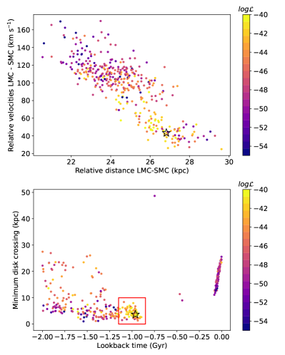
Figure 14: Top panel: present-day relative distance and velocity between the LMC and SMC in the N-body simulations. Each simulation is colour-coded according to the log-likelihood (as described in the text). Bottom panel: lookback time and the minimum radial distance $r$ of the SMC at the time it crosses the LMC’s disk. The red box marks those simulations with the largest log-likelihood, i.e., those that are a better representation of our observations.

Figure 15 shows the median in-plane radial velocity V_R and out-of-plane vertical velocity V_Z for one of the model realizations with the largest $\log{\mathcal{L}}$, and the corresponding observed velocities for each of our targets. A reasonable agreement, with a similar order of magnitude as those observed, is found for the in-plane radial velocities, while the vertical motions have larger discrepancies. The fact that there is no single model realization that is able to completely reproduce our 6D phase-space observations reflects the complex parameter space and interaction history of the past orbits of the Clouds.

Based on the radial velocities, the simulation is able to reproduce the inward motion of the MS stars and those stars in the LA group (southern outer disk). In the case of the stars on the eastern side, the northern EE stars ($\eta>$ 0°) have outwards in-plane radial motions, possibly due to being pulled out from the LMC at a different time than the stars in the north or south. South-eastern stars present both inward and outward motions, which could be explained as the result of the successive SMC’s disk crossings.

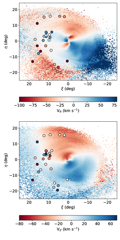
Figure 15: In-plane and out-of-plane median velocities for the particles in one of the model realizations with the largest log-likelihood, i.e, closer to the 6D phase-space observations of our targets. The individual points are all the Mira-like stars in the vicinity of the Clouds, including those potential outliers (marked with open squares in Fig. 11).

The vertical velocities of the MS stars are almost zero, being them on the LMC disk plane, while the potential outlier, MS02, has a larger positive vertical velocity. While in the case of EE stars, the vertical motion is less coherent, some stars having positive and others negative in plane velocities. LA stars have out-of-equilibrium V_z velocities, similar to the median values found in this particular model realization.

Overall, this picture in which at least two SMC’s disk crossings, besides the most recent one at $\sim$150 Myr ago, is consistent with the analysis in Cullinane et al. (2022b). In that work, the Clouds orbits were traced back up to 1 Gyr ago, and older interactions were not explored. In this work, the orbits are traced up to 2 Gyr back and even though most of the model realizations have a disk crossing more than 1.3 Gyr ago, the radial crossing distance is generally much larger than $\simeq$10 kpc. There is a small number of model realizations in which the disk crossing at $\sim$ 2 Gyr has the smallest radial crossing distance (i.e., the one that most affected the LMC disk) along the past SMC orbit. Figure 14 shows that some of them have a relatively large log-likelihood, and therefore the impact of an older disk crossing as the most important perturbation of the LMC disk cannot be fully ruled out.

Among those model realizations inside the red box in Fig. 14, which have high log-likelihood, we investigated the individual orbits of the SMC around the LMC. We found that all of those model realizations have the SMC crossing the LMC’s disk three times, at 1.8$\pm$0.6 Gyr ago, 962$\pm$32 Myr ago, and at $\sim$320$\pm$25 Myr ago. During these three times, the SMC crossed the disk of the LMC at radial crossing distances of 10.4$\pm$2.0 kpc, 4.7$\pm$1.3 kpc and 5.4$\pm$1.5 kpc, respectively. The reported values are the mean and standard deviation values based on the individual values for each of the model realizations inside the red box in Fig. 14. The standard deviations of the impact parameters are relatively low, reflecting that the past interaction histories of this sub-sample of model realizations are very similar. Based on these mean values, the radial crossing distances at $\sim$950 Myr and at $\sim$300 Myr ago are very similar, and consistent with two close pericentric passages of the SMC. The mean pericentric radial and vertical distances in this sub-sample of model realizations are r_peri = 5.2$\pm$1.3 kpc, $z_{\rm peri}$ = 5.0$\pm$1.1 kpc (at $\sim$250 Myr ago), r_peri = 4.2$\pm$1.3 kpc, $z_{\rm peri}$ = –1.2$\pm$0.4 kpc (at $\sim$950 Myr ago), and r_peri = 4.6$\pm$1.0 kpc, $z_{\rm peri}$ = –2.5$\pm$0.9 kpc (at $\sim$1.81 Gyr ago). The most recent pericentric passage is consistent with previous studies (Choi et al., 2022; Cullinane et al., 2022b) in time and pericentric distance, while the vertical distance at pericenter is similar to the values reported in Cullinane et al. (2022b). In both previous encounters, the pericentric distance of the SMC is on the order of $\sim$4.5 kpc, closer than the most recent interaction.

8 Summary and conclusions

We have carried out spectroscopic follow-up for more than 40 Mira-candidates around the LMC. Radial velocities obtained from low-resolution spectra, as well as stellar parameters, were derived for all the targets. Using Gaia DR3 parallaxes, foreground stars among our sample were discarded.

For a subsample of the remaining stars, light curves and pulsation periods were found, confirming their variable nature. After classifying the stars as C-/O-rich based on the Wesenheit functions W_BP,RP and W_J,Ks, the most likely pulsation mode was assigned based on the known distribution of LPVs around the LMC. Heliocentric distances based on PL relations were estimated for those stars with periods in the literature. We compared the distances obtained in this way with the median distance of RRL stars around each of the Mira-candidates, finding a reasonable agreement. We therefore adopted the RRL-based distance for the complete sample. The 6D phase-space information was obtained for 27 Mira candidates. For the subgroup of 14 stars located above the Galactic plane, we were not able to estimate a reliable heliocentric distance, although based on their proper motions these stars are most likely distant Galactic Miras.

A suite of N-body simulations for the LMC/SMC past interaction history (including the Milky Way) were run. From the phase-space properties of the simulated particles, the most likely simulations given our observations were identified. A scenario in which the SMC has had three close pericentric passages around the LMC seems to best resemble our observations. This particular interaction history is characterized by three LMC disk crossings of the SMC. The oldest occurred at $\sim$1.18 Gyr (impact parameter of 10.4 kpc), which is similar to the time at which a peak in the star formation history of the LMC has been found (Ruiz-Lara et al., 2020), and the expected time for the formation of the gaseous Leading Arm (Besla et al., 2010; Diaz & Bekki, 2012). After this, a second, much closer disk crossing took place at $\sim$950 Myr ago (disk crossing distance of $\sim$4.7 kpc), with this event the one that most significantly impacted the LMC periphery. A most recent disk crossing, only $\sim$350 Myr ago (disk crossing distance of $\sim$5.4 kpc) was also found to be required to recover similar kinematics to our observations.

In summary, our observations and their comparison with the N-body simulations provide a useful constraint on the past interaction history of the Clouds, in which at least three close interactions have happened, highly disturbing the motions of the stars in the LMC periphery. Our results are similar to previous studies that claimed one or two disk crossings in the last 1 Gyr, with this work studying more distant stars (relative to the LMC center), and performing a longer integration of the Clouds’s orbit (up to 2 Gyr ago). Future spectroscopic campaigns of the complete Magellanic periphery are crucial to obtain robust measurements of the stellar kinematics at different angular separations and position angles around the Clouds.

9 Data Availability and online material

All the data reduced and analyzed for the present article is fully available under reasonable request to the corresponding authors.

Appendix A Gaia DR3 parameters

Table 7 includes the Gaia source ID, parallax, stellar parameters (T_eff, log$g$, [Fe/H]) and spectral type, if available, for our targets.

Table 7: Gaia DR3 parameters for our targets. The effective temperature, surface gravity and metallicity reported are those derived from the GSP-Phot Aeneas best library using BP/RP spectra and correspond to the table columns teff_gspphot, logg_gspphot, mh_gspphot, respectively, from the gaiadr3.gaia_source table. The spectral type corresponds to the column spectraltype_esphs from the gaiadr3.astrophysical_parameters table.

ID	source ID	parallax	Teff	logg	[Fe/H]	SpType
		(mas)	(K)	(cm s-2)
BP22	5460206736750537856	0.0323	4301.4	1.8898	0.1705	K
BP23	3459149244108017408	0.0291				M
BP24	5397474650583084160	–0.0207				M
BP25	5447608326360545792	–0.0371				M
BP26	5442937635326305920	0.0011	4818.8	2.0640	–0.5251	M
BP27	5449164032234750720	0.0089				M
BP28	5672923478937609088	0.0155	33327.2	4.0456	0.0024	K
BP29	5376950032669120768	3.2880				M
BP30	3557444548542598912	3.1706				M
BP31	3571469235968627840	2.0531	3639.7	4.0367	–1.0212	M
BP32	5677088493408045568	0.0070				K
BP33	5670783966749167616	0.0361	4807.5	2.0942	–0.5508	M
BP34	3556135034489468672	2.9397	3724.6	4.5989	–0.3160	M
BP35	3483101245925708032	0.0134				K
BP36	5379917099154530944	0.0287	3410.1	0.0619	–0.4300	M
BP37	3458916766118414592	0.0249	4406.8	2.0834	0.7920	K
BP38	3477205424060762112	0.0086	4258.6	2.0246	0.2059	M
BP39	3484343968942530304	0.0027				M
EE06	5222307398713735296	–0.0231	4404.8	2.1391	0.1030	K
EE07	5273716228803929088	–0.0014				M
EE08	5287270909369746176	–0.0161	4422.5	2.6345	0.1550	K
EE09	5282142924576162816	–0.0360	4623.9	2.8845	0.3508	K
EE10	5262926244460395520	0.0073				M
EE11	5281337704108065280	0.0270	4335.3	1.8110	0.2600	K
EE12	5282659076566187776	0.0211	4503.9	2.6225	0.1709	K
EE13	5288705943842258304	0.0045	4347.6	1.8085	0.2000	K
EE14	5285751693536837376	–0.0171
EE15	5286801074305659520	0.0301	4670.9	2.7438	0.1568	K
EE16	5285520967893476224	–0.0178				CSTAR
EE17	5221807017844430592	–0.0182				M
EE18	5272890568589181952	–0.0102	4436.3	2.2757	0.1279	K
EE19	5478725879815547520	–0.0342	4546.5	2.5079	0.4875	K
EE20	5277501920355575808	0.0105	4500.4	2.6607	0.2807	K
EE21	5287009569198354816	–0.0173				M
EE22	5242317166011623808	0.0342				K
LA40	5192498745130957824	–0.0381	4327.7	2.0829	0.1371	K
LA41	5194991505491879168	–0.0063				K
LA42	5196276426565456128	–0.0170				M
LA43	5191672668300504832	–0.0044	4902.0	2.1046	–1.2015	M
LA44	4621336230122857216	–0.0028	5018.7	2.5114	–0.7710	M
MS01	4791851791893295104	–0.0500				M
MS02	5490523880100951552	–0.0229				K
MS03	5498652260326236288	–0.0514	4382.8	2.3396	0.7982	K
MS04	4768385293178232064	–0.0176	4536.1	1.7935	–0.5526	M
MS05	5499999780546395520	–0.0473				K

References

- Allende Prieto et al. (2006) Allende Prieto C., Beers T. C., Wilhelm R., Newberg H. J., Rockosi C. M., Yanny B., Lee Y. S., 2006, ApJ, 636, 804
- Allende Prieto et al. (2018) Allende Prieto C., Koesterke L., Hubeny I., Bautista M. A., Barklem P. S., Nahar S. N., 2018, A&A, 618, A25
- Belokurov & Erkal (2019) Belokurov V. A., Erkal D., 2019, MNRAS, 482, L9
- Belokurov et al. (2017) Belokurov V., Erkal D., Deason A. J., Koposov S. E., De Angeli F., Evans D. W., Fraternali F., Mackey D., 2017, MNRAS, 466, 4711
- Besla et al. (2010) Besla G., Kallivayalil N., Hernquist L., van der Marel R. P., Cox T. J., Kereš D., 2010, ApJ, 721, L97
- Bovy (2015) Bovy J., 2015, ApJS, 216, 29
- Cheng et al. (2022) Cheng X., et al., 2022, ApJ, 928, 95
- Choi et al. (2018) Choi Y., et al., 2018, ApJ, 866, 90
- Choi et al. (2022) Choi Y., Olsen K. A. G., Besla G., van der Marel R. P., Zivick P., Kallivayalil N., Nidever D. L., 2022, ApJ, 927, 153
- Cullinane et al. (2020) Cullinane L. R., et al., 2020, MNRAS, 497, 3055
- Cullinane et al. (2022a) Cullinane L. R., Mackey A. D., Da Costa G. S., Erkal D., Koposov S. E., Belokurov V., 2022a, MNRAS, 510, 445
- Cullinane et al. (2022b) Cullinane L. R., Mackey A. D., Da Costa G. S., Erkal D., Koposov S. E., Belokurov V., 2022b, MNRAS, 512, 4798
- Cullinane et al. (2023) Cullinane L. R., Mackey A. D., Da Costa G. S., Koposov S. E., Erkal D., 2023, MNRAS, 518, L25
- De Leo et al. (2020) De Leo M., Carrera R., Noël N. E. D., Read J. I., Erkal D., Gallart C., 2020, MNRAS, 495, 98
- Deason et al. (2017) Deason A. J., Belokurov V., Koposov S. E., Gómez F. A., Grand R. J., Marinacci F., Pakmor R., 2017, MNRAS, 470, 1259
- Di Teodoro et al. (2019) Di Teodoro E. M., et al., 2019, MNRAS, 483, 392
- Diaz & Bekki (2012) Diaz J. D., Bekki K., 2012, ApJ, 750, 36
- Drake et al. (2017) Drake A. J., et al., 2017, MNRAS, 469, 3688
- El Youssoufi et al. (2021) El Youssoufi D., et al., 2021, MNRAS, 505, 2020
- Erkal et al. (2019) Erkal D., et al., 2019, MNRAS, 487, 2685
- Gaia Collaboration et al. (2021) Gaia Collaboration et al., 2021, A&A, 649, A7
- Gaia Collaboration et al. (2022) Gaia Collaboration et al., 2022, arXiv e-prints, p. arXiv:2208.00211
- Gatto et al. (2022) Gatto M., Ripepi V., Bellazzini M., Tortora C., Tosi M., Cignoni M., Longo G., 2022, ApJ, 931, 19
- Gillet et al. (1985) Gillet D., Ferlet R., Maurice E., Bouchet P., 1985, A&A, 150, 89
- Graczyk et al. (2014) Graczyk D., et al., 2014, ApJ, 780, 59
- Harris & Zaritsky (2006) Harris J., Zaritsky D., 2006, AJ, 131, 2514
- Hernquist (1990) Hernquist L., 1990, ApJ, 356, 359
- Jayasinghe et al. (2018) Jayasinghe T., et al., 2018, MNRAS, 477, 3145
- Joy (1926) Joy A. H., 1926, ApJ, 63, 281
- Kallivayalil et al. (2013) Kallivayalil N., van der Marel R. P., Besla G., Anderson J., Alcock C., 2013, ApJ, 764, 161
- Koesterke et al. (2008) Koesterke L., Allende Prieto C., Lambert D. L., 2008, ApJ, 680, 764
- Lebzelter et al. (2018) Lebzelter T., Mowlavi N., Marigo P., Pastorelli G., Trabucchi M., Wood P. R., Lecoeur-Taïbi I., 2018, A&A, 616, L13
- Lebzelter et al. (2019) Lebzelter T., Trabucchi M., Mowlavi N., Wood P. R., Marigo P., Pastorelli G., Lecoeur-Taïbi I., 2019, A&A, 631, A24
- Mackey et al. (2016) Mackey A. D., Koposov S. E., Erkal D., Belokurov V., Da Costa G. S., Gómez F. A., 2016, MNRAS, 459, 239
- Mackey et al. (2018) Mackey D., Koposov S., Da Costa G., Belokurov V., Erkal D., Kuzma P., 2018, ApJ, 858, L21
- Martini et al. (2014) Martini P., et al., 2014, in Ramsay S. K., McLean I. S., Takami H., eds, Society of Photo-Optical Instrumentation Engineers (SPIE) Conference Series Vol. 9147, Ground-based and Airborne Instrumentation for Astronomy V. p. 91470Z (arXiv:1407.4541), doi:10.1117/12.2056834
- Menzies et al. (2006) Menzies J. W., Feast M. W., Whitelock P. A., 2006, MNRAS, 369, 783
- Niederhofer et al. (2021) Niederhofer F., et al., 2021, MNRAS, 502, 2859
- Niederhofer et al. (2022) Niederhofer F., et al., 2022, MNRAS, 512, 5423
- Olsen & Salyk (2002) Olsen K. A. G., Salyk C., 2002, AJ, 124, 2045
- Olsen et al. (2011) Olsen K. A. G., Zaritsky D., Blum R. D., Boyer M. L., Gordon K. D., 2011, ApJ, 737, 29
- Petersen et al. (2022) Petersen M. S., Peñarrubia J., Jones E., 2022, MNRAS, 514, 1266
- Pietrzyński et al. (2019) Pietrzyński G., et al., 2019, Nature, 567, 200
- Ripepi et al. (2017) Ripepi V., et al., 2017, MNRAS, 472, 808
- Ruiz-Lara et al. (2020) Ruiz-Lara T., et al., 2020, A&A, 639, L3
- Skrutskie et al. (2006) Skrutskie M. F., et al., 2006, AJ, 131, 1163
- Soszynski et al. (2007) Soszynski I., et al., 2007, Acta Astron., 57, 201
- Stanimirović et al. (2004) Stanimirović S., Staveley-Smith L., Jones P. A., 2004, ApJ, 604, 176
- Tody (1993) Tody D., 1993, in Hanisch R. J., Brissenden R. J. V., Barnes J., eds, Astronomical Society of the Pacific Conference Series Vol. 52, Astronomical Data Analysis Software and Systems II. p. 173
- Tonry & Davis (1979) Tonry J., Davis M., 1979, AJ, 84, 1511
- Vasiliev (2019) Vasiliev E., 2019, MNRAS, 482, 1525
- Wan et al. (2020) Wan Z., Guglielmo M., Lewis G. F., Mackey D., Ibata R. A., 2020, MNRAS, 492, 782
- Wright et al. (2010) Wright E. L., et al., 2010, AJ, 140, 1868
- Zhao & Evans (2000) Zhao H., Evans N. W., 2000, ApJ, 545, L35
- de Vaucouleurs & Freeman (1972) de Vaucouleurs G., Freeman K. C., 1972, Vistas in Astronomy, 14, 163
- van der Marel & Cioni (2001) van der Marel R. P., Cioni M.-R. L., 2001, AJ, 122, 1807
- van der Marel & Kallivayalil (2014) van der Marel R. P., Kallivayalil N., 2014, ApJ, 781, 121
- van der Marel et al. (2002) van der Marel R. P., Alves D. R., Hardy E., Suntzeff N. B., 2002, AJ, 124, 2639