Delay-Adaptive Compensator for 3-D Space Formation of Multi-Agent Systems with Leaders Actuation

Abstract

This paper focuses on the control of collective dynamics in large-scale multi-agent systems (MAS) operating in a 3-D space, with a specific emphasis on compensating for the influence of an unknown delay affecting the actuated leaders. The communication graph of the agents is defined on a mesh-grid 2-D cylindrical surface. We model the agents’ collective dynamics by a complex- and a real-valued reaction-advection-diffusion 2-D partial differential equations (PDEs) whose states represent the 3-D position coordinates of the agents. The leader agents on the boundary suffer unknown actuator delay due to the cumulative computation and information transmission time. We design a delay-adaptive controller for the 2-D PDE by using PDE backstepping combined with a Lyapunov functional method, where the latter is employed to design an update law that generates real-time estimates of the unknown delay. Capitalizing on our recent result on the control of 1-D parabolic PDEs with unknown input delay, we use Fourier series expansion to bridge the control of 1-D PDEs to that of 2-D PDEs. To design the update law for the 2-D system, a new target system is defined to establish the closed-loop local boundedness of the system trajectories in $H^{2}$ norm and the regulation of the states to zero assuming a measurement of the spatially distributed plant’s state. We illustrate the performance of delay-adaptive controller by numerical simulations.

, ,

1 Introduction

Cooperative formation control in multi-agent systems (MAS) has garnered substantial interest due to its wide-ranging applications in various engineering domains, such as UAV formation flying [3], multi-robot collaboration [2, 25], vehicle queues [5], and satellite clusters [32]. In MASs, communication delays, stemming from information exchange between agents, and input delays, arising from the processing/aquisition of data to update feedback control signals, can frequently lead to “suboptimal” performance and, in more critical cases, potentially result in system instability. Over the past few decades, there has been a significant body of research in multi-agent systems focusing on communication delays. This research has predominantly employed high-order models and consensus protocols [9, 31]. In the context of non-uniform communication delays, [12] establish the critical role of a globally reachable node in the information graph when designing linear agreement protocols for agents [12]. The authors of [23] employ frequency domain analysis to derive a delay-dependent consensus condition for a first-order multi-agent system with input and communication delays. In [34], a triggering mechanism is introduced to establish a necessary and sufficient condition for leader-following consensus in multi-agent systems with input delays, while a comparable condition for second-order consensus in multi-agent dynamical systems with input delays is introduced in [31]. Using the Artstein-Kwon-Pearson reduction method to convert delay-dependent systems into delay-free systems, fixed-time event-triggered consensus for linear MAS with input delay is achieved in [1]. Based on a Lyapunov method for a mean square consensus problem of leader-following stochastic MAS with input time-dependent or constant delay, [21] provide sufficient conditions to achieving consensus. A solution for leader-follower consensus in nonlinear multi-agent systems with unknown nonuniform time-varying input delay is provided in [13] by constructing a delay-independent output-feedback controller for each follower. While the prevalent focus in the literature has been on the impact of input delay on follower agents, [18] address a known delay affecting the actuated leaders within a 3-D infinite-dimensional framework. Furthermore, most of these studies rely on ordinary differential equations (ODEs) models, namely, each agent’s dynamic state is represented by an ODE, resulting in increased system complexity as the number of agents grows [12, 14].

For multi-agent systems, control designs using partial differential equations (PDEs) provide a compact representation for capturing the dynamics of large-scale systems. These PDEs, whether they take a parabolic or hyperbolic form, describe the position coordinates of individual agents, as demonstrated in various works including [16, 7, 8, 17, 19] and the reference therein. In the case of parabolic systems, the diffusion term, namely, the Laplace operator plays the role of MAS consensus protocol modeled by ODEs. Actuation of the leader agents positioned on the periphery of the communication structure demands a greater amount of information and computational resources compared to the follower agents. Consequently, leaders are more susceptible to delays that affect the formation control. Using the nominal delay-compensated boundary control law proposed in [11, 29], the authors of [18] designed a boundary feedback law for MAS in 3-D space under a constant and known input delay. However, in practical scenarios, knowing precisely the value of the delay is often unfeasible, and instead, it is possible to estimate only its upper and lower bounds. To overcome such a challenge, the authors of [15] investigate the determination of the delay bounds within which regulated state synchronization is attainable for a multi-agent system with unknown and nonuniform input delays. Similarly, in [33], such a delay bound is characterized for semi-global state synchronization in a multi-agent system with actuator saturation and unknown nonuniform input delays. Nevertheless, there is a dearth of literature that addresses the issue of unknown delays in the context of multi-agent systems modeled by partial differential equations (PDEs). For a reaction-diffusion systems subject to an unknown boundary input delays [28] pioneering exploration led to a delay-adaptive compensated controller that ensures the regulation of the system’s state to zero. Motivated by decontamination of a polluted surface, [27] constructed a delay-adaptive predictor feedback for reaction-diffusion systems subject to a delayed distributed input. The stabilization of deep-sea construction vessels using Batch-Least Squares Identifiers [10] has been achieved in [26] where finite-time exact identification of an unknown boundary input delay and simultaneously exponential regulation of the plant’s state for a hyperbolic PDE-ODE system is ensured. More recently, a Lyapunov design approach that enables global stability for a hyperbolic PIDE (Partial Integro-Differential Equation) with an unknown boundary input delay was introduced in [30].

We consider a formation control in 3-D space of a multi-agent system with unknown actuator delay. The collective dynamics of the MAS is modeled by two diffusion 2-D PDEs; one is a complex-valued PDE whose states represent the agents’ positions in coordinates $(x,y)$ and the other is a real-valued PDE whose states represent the agents’ positions in coordinate $z$. We utilize PDE backstepping design in conjunction with a Lyapunov method to construct a dynamic delay-adaptive boundary feedback law. The nominal backstepping controller acquires complementary information about the unknown parameter through an update law driven by a carefully designed ODE. Our present work potentially marks a pioneering contribution in the field of PDE-based formation control for multi-agent systems with unknown input delays in three-dimensional space. We introduce Fourier series expansion to reduce the dimensionality of the 2-D system to $n$ 1-D systems. In contrast to the result in [18], the target system in the present study accounts for several highly nonlinear terms, generated by the delay-adaptive scheme, which pose challenges in establishing the convergence of their series representations, a crucial prerequisite for transforming the 1-D system into a 2-D system.

This paper is organized as follows. Section 2 introduces the PDE-based model for a MAS with actuation delay. Section 3 presents the delay-adaptive control design for the MAS collective dynamics subject to unknown actuation delay. The design of the delay’s adaptation law and the local stability analysis of the MAS are presented in Section 4 and Section 5, respectively. Simulation results are provided in Section 6. The paper concludes with a discussion possible of future works in Section 7.

Notation: Throughout the paper, we adopt the following notation for $\chi(\theta,s)$ on the cylindrical surface [22, 18]:

The $L^{2}$ norm is defined as

$$||\chi(s,\theta)||_{L^{2}}=\left(\int_{0}^{1}\int_{-\pi}^{\pi}|\chi(s,\theta)|^{2}\mathrm{d}\theta\mathrm{d}s\right)^{\frac{1}{2}},$$ (1)

for $\chi(\theta,s)\in L^{2}((0,1)\times(-\pi,\pi))$. To save space, we set $\rVert\chi\rVert^{2}=\rVert\chi(s,\theta)\rVert^{2}_{L^{2}}$. The Sobolev norm $||\centerdot||_{H^{1}}$ is defined as $||\chi||^{2}_{H^{1}}=\|\chi\|^{2}+\|\partial_{s}\chi\|^{2}+\|\partial_{\theta}\chi\|^{2}$ for $\chi(\theta,s)\in H^{1}((0,1)\times(-\pi,\pi))$. The Sobolev norm $||\centerdot||_{H^{2}}$ is defined as $||\chi||^{2}_{H^{2}}=\|\chi\|_{H^{1}}^{2}+\|\partial^{2}_{s}\chi\|^{2}+2\|\partial_{s\theta}\chi\|^{2}+\|\partial^{2}_{\theta}\chi\|^{2}$ for $\chi(\theta,s)\in H^{2}((0,1)\times(-\pi,\pi))$.

2 Muilt-Agent’s PDEs Model

2.1 Model description

Following [18], we consider a group of agents located on a cylindrical surface undirected topology graph with index $(i,j),~{}i=1,...,\ M,~{}j=1,...,N$, moving in a 3-D space under the coordinate axes $(x,y,z)$. A complex-valued state $u=x+\mathrm{j}y$ is defined to simplify the expression of the components on the $(x,y)$ axes. Defining the discrete indexes $(i,j)$ of the agents into a continuous domain, $\Omega=\{(s,\theta):0<{s}<{1}$, $-\pi\leq{\theta}\leq{\pi}\}$, as $M,~{}N\to{\infty}$ (see, Figure 1), the continuum model of the collective dynamics of a large scale multi-agent system as follows

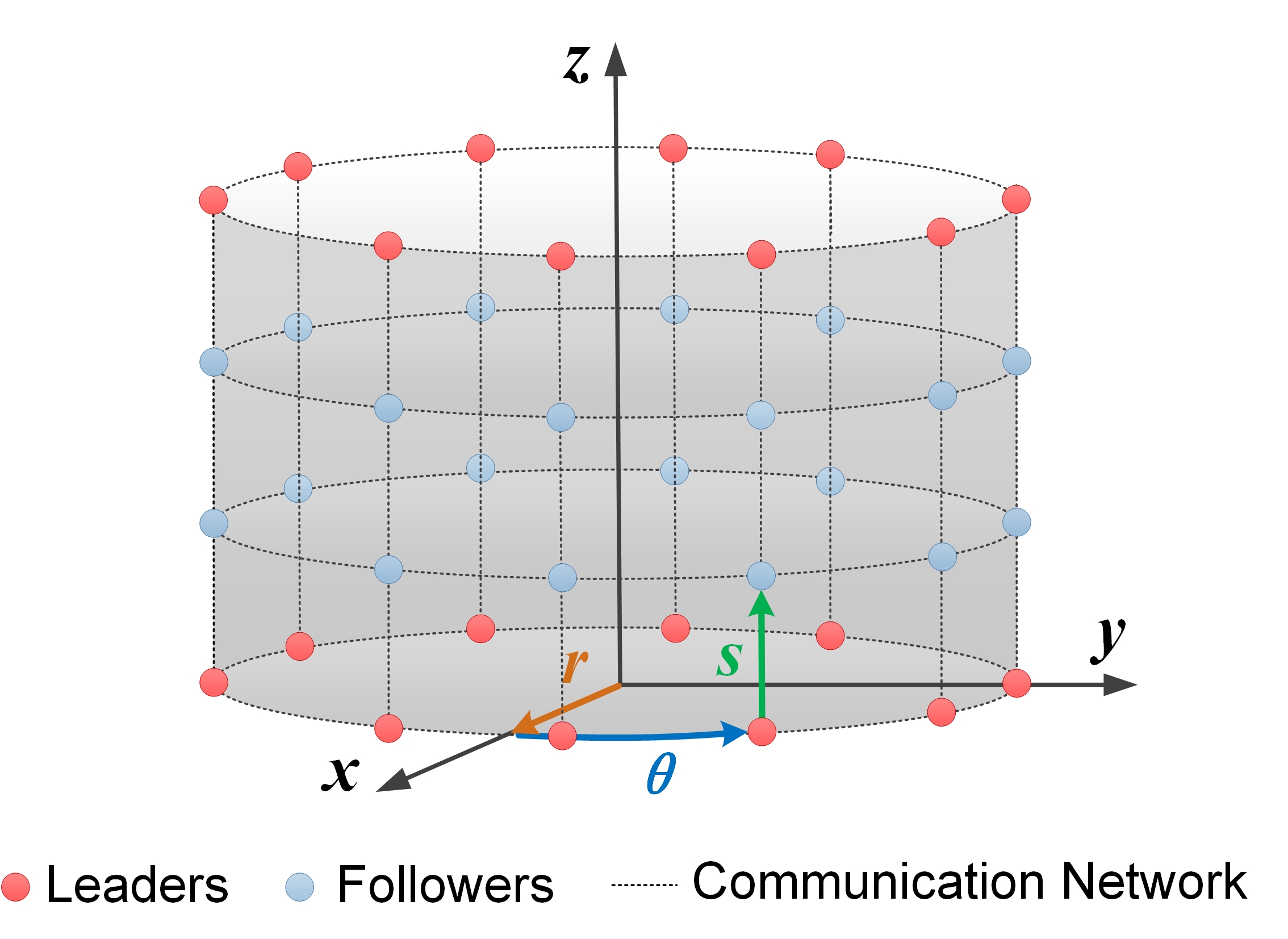
Figure 1: Cylindrical surface topology prescribing the communication relationship among agents. The agents at the uppermost and lowermost layers are leaders. Each follower has four neighbors.

$${\partial}_{t}u(s,{\theta},t)={\Delta}{u}(s,{\theta},t)+\beta_{1}{\partial}_{s}u(s,{\theta},t)+{\lambda_{1}}{u}(s,{\theta},t),$$ (2)

$${\partial}_{t}{z}(s,{\theta},t)={\Delta}{z}(s,{\theta},t)+\beta_{2}{\partial}_{s}z(s,{\theta},t)+{\lambda_{2}}{z}(s,{\theta},t),$$ (3)

$${\color[rgb]{0,0,0}(s,-\pi,t)={u}(s,\pi,t)},\quad{u}(0,{\theta},t)=f_{1}(\theta),$$ (4)

$${u}(1,{\theta},t)=g_{1}(\theta)+{U}({\theta},t-D),$$ (5)

$${\color[rgb]{0,0,0}(s,-\pi,t)={z}(s,\pi,t)},\quad{z}(0,{\theta},t)=f_{2}(\theta),$$ (6)

$${z}(1,{\theta},t)=g_{2}(\theta)+{Z}({\theta},t-D),$$ (7)

where $(s,{\theta},t)\in\Omega\times{\mathbb{R}^{+}}$, $u$, $\lambda_{1}$, $\beta_{1}\in{\mathbb{C}}$, $z$, $\lambda_{2}$, $\beta_{2}\in{\mathbb{R}}$. The coordinates $(s,\theta)$ are the spatial variables denoting the indexes of the agents in the continuum and ${\Delta}$ represents the following Laplace operator

$${\Delta}{u}(s,{\theta},t) ={\partial}^{2}_{s}u(s,{\theta},t)+{\partial}^{2}_{\theta}u(s,{\theta},t),$$ (8)

$${\Delta}{z}(s,{\theta},t) ={\partial}^{2}_{s}z(s,{\theta},t)+{\partial}^{2}_{\theta}z(s,{\theta},t),$$ (9)

which is defined as ”consensus operators” for PDE representations [6]. Note that the boundary conditions (4) and (6) are periodical on the cylinder surface (see Figure 1) while $f_{1}(\theta)$, $g_{1}(\theta)$, $f_{2}(\theta)$ and $g_{2}(\theta)$ are non-zero bounded boundary conditions for the states $u$ and $z$, respectively.

To control the MAS to desired formations, we consider a configuration where the agents at the boundaries $s=0$ and $s=1$ are the leaders that drive all the agents to prescribe equilibrium. In (5) and (7), we defined the input delay $D>0$ affecting the actuated leaders and caused by communication lags in leader-follower configurations. In practice, the exact value of the delay is hard to measure, only the bounds of the unknown delay can be estimated, so we assume:

Assumption 1.

Assume delay $D\in\{D\in\mathbb{R}^{+}|\underline{D}\leq D\leq\overline{D}\}$, where $\underline{D}$ and $\overline{D}$ are the known lower and upper bounds, respectively.

Remark 1.

Letting $\partial_{t}u(s,\theta,t)=0$ and $\partial_{t}z(s,\theta,t)=0$, one can solve (2)–(7) without control and get steady state profiles $\bar{u}(s,\theta)$ and $\bar{z}(s,\theta)$, which express the desired formations as functions of the values of the parameters $\lambda_{1}$, $\beta_{1}$, $\lambda_{2}$, $\beta_{2}$ and the open-loop boundary conditions $f_{1}(\theta)$, $g_{1}(\theta)$, $f_{2}(\theta)$ and $g_{2}(\theta)$ [18].

3 Delay-adaptive boundary controller design

First, define the error between the actual system and the desired system as $\tilde{u}(s,{\theta},t)=u(s,{\theta},t)-\bar{u}(s,{\theta})$, and then introduce a change of variable $\phi(s,{\theta},t)=e^{\frac{1}{2}\beta_{1}s}\tilde{u}(s,{\theta},t)$ for removing the convection term,

$$\partial_{t}{\phi}(s,{\theta},t)={\Delta}{\phi}(s,{\theta},t)+{\lambda^{\prime}_{1}}{\phi}(s,{\theta},t),~{}~{}s\in(0,1),$$ (10)

$${\color[rgb]{0,0,0}(s,-\pi,t)={\phi}(s,\pi,t)},\quad{\phi}(0,{\theta},t)=0,$$ (11)

$${\phi}(1,{\theta},t)=\Phi(\theta,t-D),$$ (12)

where $\lambda^{\prime}_{1}=\lambda_{1}-\frac{1}{4}\beta_{1}^{2}$ and ${\Phi}({\theta},t-D)=e^{\frac{1}{2}\beta_{1}}{U}({\theta},t-D)$. By employing a transport PDE of $\vartheta$ representation of the delay appearing in (5), we transform the error system (10)–(12) as follows:

$$\partial_{t}{\phi}(s,{\theta},t)={\Delta}{\phi}(s,{\theta},t)+{\lambda^{\prime}_{1}}{\phi}(s,{\theta},t),~{}~{}s\in(0,1),$$ (13)

$${\color[rgb]{0,0,0}(s,-\pi,t)={\phi}(s,{\pi},t)},\quad{\phi}(0,{\theta},t)=0,$$ (14)

$${\phi}(1,{\theta},t)={\vartheta}(0,{\theta},t),$$ (15)

$$D\partial_{t}{\vartheta}(s,{\theta},t)=\partial_{s}{\vartheta}(s,{\theta},t),$$ (16)

$${\color[rgb]{0,0,0}\vartheta(s,{-\pi},t)=\vartheta(s,\pi,t)},\quad\vartheta(1,{\theta},t)=\Phi(\theta,t),$$ (17)

where $\vartheta(s,{\theta},t)=\Phi({\theta},t+D(s-1))$, defined in $\Omega\times\mathbb{R}^{+}$. In the following, we will adopt the design method presented in [18] to derive the dynamic boundary adaptive controller of the states $u$ and $z$ but limit our analysis to the $u$ component of the state as a similar approach applies for the $z$ dynamics.

3.1 Fourier series expansions

In order to transform the 2-D system (13)–(17) into $n$ 1-D systems, we introduce the Fourier series expansion [24] as

$${\phi}(s,{\theta},t)=\sum_{n=-\infty}^{\infty}{\phi}_{n}(s,t)e^{\mathrm{j}n\theta},~{}~{}$$ (18)

$${\Phi}({\theta},t)=\sum_{n=-\infty}^{\infty}{\Phi}_{n}(t)e^{\mathrm{j}n\theta},$$ (19)

$${\vartheta}(s,{\theta},t)=\sum_{n=-\infty}^{\infty}{\vartheta}_{n}(s,t)e^{\mathrm{j}n\theta},$$ (20)

where $\phi_{n}$, $\Phi_{n}$, ${\vartheta}_{n}$ are the $n$ Fourier coefficients; independent of the angular argument $\theta$. As an illustration, one of the coefficients in (18)–(20) is given as $\phi_{n}(s,t)=\frac{1}{2\pi}\int_{-\pi}^{\pi}\phi(s,\psi,t)e^{-\mathrm{j}n\psi}\mathrm{d}\psi$. Introducing (18)–(20) to (13)–(17), we get the following 1-D PDE of the Fourier coefficients ${\phi}_{n}(s,t)$ and ${\vartheta}_{n}(s,t)$

$$\partial_{t}{\phi}_{n}(s,t)=\partial^{2}_{s}{\phi}_{n}(s,t)+(\lambda^{\prime}_{1}-n^{2}){\phi}_{n}(s,t),~{}s\in(0,1),$$ (21)

$${\phi}_{n}(0,t)=0,\quad{\phi}_{n}(1,t)={\vartheta}_{n}(0,t),$$ (22)

$$D\partial_{t}{\vartheta}_{n}(s,t)={\partial_{s}}{\vartheta}_{n}(s,t),\quad{\vartheta}_{n}(1,t)={\Phi}_{n}(t).$$ (23)

We design a feedback adaptive controller $\Phi_{n}$ to stabilize each cascade system $(\phi_{n},\vartheta_{n})$ in (21)–(23) by postulating the following transformations

$${w}_{n}(s,t) =\mathcal{T}_{n}[\phi_{n}](s,t)={\phi}_{n}(s,t)-\int_{0}^{s}k_{n}(s,\tau)\phi_{n}(\tau,t)\mathrm{d}\tau,$$ (24)

$${h}_{n}(s,t) =\mathcal{T}_{n}[\vartheta_{n}](s,t)={-\hat{D}(t)}\int_{0}^{s}p_{n}(s,\tau,\hat{D}(t))\vartheta_{n}(\tau,t)\mathrm{d}\tau$$

$$+{\vartheta}_{n}(s,t)-\int_{0}^{1}\gamma_{n}(s,\tau,\hat{D}(t))\phi_{n}(\tau,t)\mathrm{d}\tau,$$ (25)

with the inverse transformations

$${\phi}_{n}(s,t) =\mathcal{T}_{n}^{-1}[w_{n}](s,t)={w}_{n}(s,t)+\int_{0}^{s}l_{n}(s,\tau)w_{n}(\tau,t)\mathrm{d}\tau,$$ (26)

$${\vartheta}_{n}(s,t) =\mathcal{T}_{n}^{-1}[h_{n}](s,t)={\hat{D}(t)}\int_{0}^{s}q_{n}(s,\tau,\hat{D}(t))h_{n}(\tau,t)\mathrm{d}\tau$$

$$+h_{n}(s,t)+\int_{0}^{1}\eta_{n}(s,\tau,\hat{D}(t))w_{n}(\tau,t)\mathrm{d}\tau,$$ (27)

where the kernels are defined on ${\mathcal{D}}=\{(s,\tau,\hat{D}(t)):0\leq\tau\leq s\leq 1\}$, and $\hat{D}(t)$ is the estimate of unknown input delay.

Hence, by PDE Backstepping method, (21)–(23) maps into the following target system parameterized by $\hat{D}=\tilde{D}-D$

$$\partial_{t}{w}_{n}(s,t)=\partial^{2}_{s}{w}_{n}(s,t)-n^{2}{w}_{n}(s,t),$$ (28)

$${w}_{n}(0,t)=0,\quad{w}_{n}(1,t)={h}_{n}(0,t),$$ (29)

$$D{\partial_{t}h}_{n}(s,t)={\partial_{s}h}_{n}(s,t)-\tilde{D}P_{1n}(s,t)-D\dot{\hat{D}}P_{2n}(s,t),$$ (30)

$${h}_{n}(1,t)=0,$$ (31)

where

$$P_{1n} (s,t)=\int_{0}^{1}\bigg{(}-{\partial_{\tau}}\gamma_{n}(s,1,\hat{D})l_{n}(1,\tau)+\frac{1}{\hat{D}}\partial_{s}\gamma_{n}(s,\tau,\hat{D})$$

$$+\frac{1}{\hat{D}}\int_{\tau}^{1}\partial_{s}\gamma_{n}(s,\tau,\hat{D})l_{n}(\xi,t)\mathrm{d}\xi\bigg{)}w_{n}(\tau,t)\mathrm{d}\tau$$

$$-{\partial_{\tau}}\gamma_{n}(s,1,\hat{D})h_{n}(0,t),$$ (32)

$$P_{2n} (s,t)=\int_{0}^{1}\bigg{(}\int_{\tau}^{1}\partial_{{\hat{D}}}\gamma_{n}(s,\tau,\hat{D})l_{n}(\xi,\tau)\mathrm{d}\xi+\partial_{{\hat{D}}}\gamma_{n}(s,\tau,\hat{D})$$

$$+\int_{0}^{s}(p_{n}(s,\xi,\hat{D})+{\hat{D}}\partial_{{\hat{D}}}p_{n}(s,\xi,\hat{D}))\eta_{n}(\xi,\tau,\hat{D})\mathrm{d}\xi\bigg{)}$$

$$\cdot w_{n}(\tau,t)\mathrm{d}\tau+\int_{0}^{s}\bigg{(}{\hat{D}}\partial_{{\hat{D}}}p_{n}(s,\tau,\hat{D})+p_{n}(s,\tau,\hat{D})$$

$$+\hat{D}\int_{\tau}^{s}(p_{n}(s,\xi,\hat{D})+{\hat{D}}\partial_{{\hat{D}}}p_{n}(s,\xi,\hat{D}))q_{n}(\xi,\tau,\hat{D})\mathrm{d}\xi\bigg{)}$$

$$\cdot h_{n}(\tau,t)\mathrm{d}\tau.$$ (33)

The mapping (24), (3.1) is well defined if the kernel functions $k_{n}(s,\tau)$, $\gamma_{n}(s,\tau)$ and $p_{n}(s,\tau)$ satisfy

$$\partial^{2}_{s}{k}_{n}(s,\tau)=\partial^{2}_{\tau}{k}_{n}(s,\tau)+\lambda^{\prime}_{1}{k}_{n}(s,\tau),$$ (34)

$${k}_{n}(s,0)=0,\quad{k}_{n}(s,s)=-\frac{\lambda^{\prime}_{1}}{2}s,$$ (35)

$$\partial_{s}{\gamma}_{n}(s,\tau,\hat{D})=\hat{D}(\partial^{2}_{\tau}{\gamma}_{n}(s,\tau,\hat{D})+(\lambda^{\prime}_{1}-n^{2}){\gamma}_{n}(s,\tau,\hat{D})),$$ (36)

$${\gamma}_{n}(s,0,\hat{D})={\gamma}_{n}(s,1,\hat{D})=0,\quad{\gamma}_{n}(0,\tau,\hat{D})={k}_{n}(1,\tau),$$ (37)

$$\partial_{s}p_{n}(s,\tau,\hat{D})=-\partial_{\tau}p_{n}(s,\tau,\hat{D}),$$ (38)

$$p_{n}(s,1,\hat{D})=-\partial_{\tau}{\gamma}_{n}(s,\tau,\hat{D})|_{\tau=1}.$$ (39)

The solution of the above gain kernels PDEs is given by

$${k}_{n}(s,\tau)=-\lambda\tau\frac{I_{1}(\sqrt{\lambda^{\prime}_{1}(s^{2}-{\tau}^{2})})}{\sqrt{\lambda^{\prime}_{1}(s^{2}-{\tau}^{2})}},$$ (40)

$$\gamma_{n}(s,\tau,\hat{D})=2\sum_{i=1}^{\infty}e^{\hat{D}(\lambda^{\prime}_{1}-n^{2}-i^{2}{\pi^{2}})s}{\mathrm{sin}}(i\pi\tau)\int_{0}^{1}{\mathrm{sin}}(i\pi\xi)$$

$$~{}~{}~{}~{}~{}~{}~{}~{}~{}~{}~{}~{}~{}~{}~{}~{}~{}\cdot k(1,\xi){\mathrm{d}{\xi}},$$ (41)

$${p}_{n}(s,\tau,\hat{D})=-{\partial}_{2}{\gamma}_{n}(s-\tau,1,\hat{D}),$$ (42)

where $\partial_{2}\gamma_{n}(\cdot,\cdot,\cdot)$ denotes the derivative of $\gamma_{n}(\cdot,\cdot,\cdot)$ with respect to the second argument. Similarly, one can get the kernels in inverse transformations (26), (3.1):

$${l}_{n}(s,\tau)=-\lambda\tau\frac{J_{1}(\sqrt{\lambda^{\prime}_{1}(s^{2}-{\tau}^{2})})}{\sqrt{\lambda^{\prime}_{1}(s^{2}-{\tau}^{2})}},$$ (43)

$$\eta_{n}(s,\tau,\hat{D})=2\sum_{i=1}^{\infty}e^{-\hat{D}(n^{2}+i^{2}\pi^{2})s}{\mathrm{sin}}(i\pi\tau)\int_{0}^{1}{\mathrm{sin}}(i\pi\xi)$$

$$~{}~{}~{}~{}~{}~{}~{}~{}~{}~{}~{}~{}~{}~{}~{}~{}~{}\cdot k(1,\xi){\mathrm{d}{\xi}},$$ (44)

$${q}_{n}(s,\tau,\hat{D})=-{\partial}_{2}{\eta}_{n}(s-\tau,1,\hat{D}).$$ (45)

From (23), (3.1) and (31), the 1-D delay-compensated adaptive controller writes

$${{\color[rgb]{0,0,0}\Phi}}_{n}(t)= {\hat{D}}\int_{0}^{1}p_{n}(1,\tau,\hat{D})\vartheta_{n}(\tau,t)\mathrm{d}\tau$$

$$+\int_{0}^{1}\gamma_{n}(1,\tau,\hat{D})\phi_{n}(\tau,t)\mathrm{d}\tau.$$ (46)

3.2 2-D delay-compensated adaptive controller

In order to obtain the 2-D delay-compensated adaptive controller, we assemble all the $n$ 1-D transformations defined in (24)–(3.1) in the form of Fourier series to recover the 2-D domain components and then get

$$w(s,\theta,t) {=\sum_{n=-\infty}^{\infty}{w}_{n}(s,t)e^{\mathrm{j}n\theta}}$$

$$={\phi}(s,\theta,t)-\int_{0}^{s}{k}(s,\tau){\phi}(\tau,\theta,t){\mathrm{d}{\tau}},$$ (47)

$${h}(s,{\theta},t) {=\sum_{n=-\infty}^{\infty}h_{n}(s,t)e^{\mathrm{j}n\theta}}={\vartheta}(s,{\theta},t)$$

$$-\int_{0}^{1}\int_{-\pi}^{\pi}\gamma(s,\tau,\theta,\psi,\hat{D})w(\tau,\psi,t)\mathrm{d}\psi\mathrm{d}\tau$$

$$-\hat{D}\int_{0}^{s}\int_{-\pi}^{\pi}p(s,\tau,\theta,\psi,\hat{D})\vartheta(\tau,\psi,t)\mathrm{d}\psi\mathrm{d}\tau,$$ (48)

where $k(s,\tau)$ is defined in (40), the related 2-D kernels are given as

$$\gamma(s,\tau,\theta,\psi,\hat{D})= 2{Q(s,\theta-\psi,\hat{D})}\sum_{i=1}^{\infty}e^{\hat{D}(\lambda^{\prime}_{1}-i^{2}\pi^{2})s}\mathrm{sin}(i\pi\tau)$$

$$\cdot\int_{0}^{1}\mathrm{sin}(i\pi\xi)k(1,\xi)\mathrm{d}\xi,$$ (49)

$$p(s,\tau,\theta,\psi,\hat{D})= -\partial_{2}\gamma(s-\tau,1,\theta-\psi,\hat{D}).$$ (50)

For all $s\in[0,1]$, defining ${Q(s,\theta-\psi,\hat{D})}=\frac{1}{2\pi}\sum_{n=-\infty}^{\infty}e^{-\hat{D}n^{2}s}$
$\cdot e^{\mathrm{j}n(\theta-\psi)}$. Due to $0<Q(s,\theta-\psi,\hat{D})\leq P(e^{-\hat{D}s},\theta-\psi)$, where $P$ denotes Possion Kernel. Using the properties of Poisson kernels [4], one gets the boundedness of the kernel functions $\gamma(s,\tau,\theta,\psi,\hat{D})$ and $p(s,\tau,\theta,\psi,\hat{D})$. In a similar way, we get the inverse transformations of (3.2) and (48) are given by

$${\phi}(s,{\theta},t)={w}(s,{\theta},t)+\int_{0}^{s}l(s,\tau)w(\tau,{\theta},t)\mathrm{d}\tau,$$ (51)

$${\vartheta}(s,{\theta},t)=\int_{0}^{1}\int_{-\pi}^{\pi}\eta(s,\tau,\theta,\psi,\hat{D})w(\tau,\psi,t)\mathrm{d}\psi\mathrm{d}\tau$$

$${+h}(s,{\theta},t)+\hat{D}\int_{0}^{s}\int_{-\pi}^{\pi}q(s,\tau,\theta,\psi,\hat{D})h(\tau,\psi,t)\mathrm{d}\psi\mathrm{d}\tau,$$ (52)

where the gain kernels $l$, $q$ and $\eta$ are defined as

$$l(s,\tau)=-\lambda\tau\frac{J_{1}(\sqrt{\lambda^{\prime}_{1}(s^{2}-{\tau}^{2})})}{\sqrt{\lambda^{\prime}_{1}(s^{2}-{\tau}^{2})}},\quad$$ (53)

$$\eta(s,\tau,\theta,\psi,\hat{D})=2{Q(s,\theta-\psi,\hat{D})}\sum_{i=1}^{\infty}e^{-\hat{D}i^{2}\pi^{2}s}\mathrm{sin}(i\pi\tau)$$

$$~{}~{}~{}~{}~{}~{}~{}~{}~{}~{}~{}~{}~{}~{}~{}~{}~{}~{}~{}~{}~{}~{}~{}~{}\cdot\int_{0}^{1}\mathrm{sin}(i\pi\xi)l(1,\xi)\mathrm{d}\xi,$$ (54)

$$q(s,\tau,\theta,\psi,\hat{D})=-{\partial_{2}}{\eta}(s-\tau,1,\theta,\psi,\hat{D}).$$ (55)

From (3.1), (3.2) and (50), we obtain the following delay-adaptive control law:

$$U({\theta},t)=\int_{0}^{1}\int_{-\pi}^{\pi}\gamma(1,\tau,\theta,\psi,\hat{D})e^{-\frac{1}{2}\beta_{1}(1-\tau)}(u(\tau,{\psi},t)$$

$$~{}~{}~{}~{}-\bar{u}(\tau,{\psi}))\mathrm{d}\psi\mathrm{d}\tau-\int_{t-D}^{t}\int_{-\pi}^{\pi}{\partial_{2}}{\gamma}(\frac{t-\nu}{\hat{D}},1,\theta,\psi,\hat{D})e^{\frac{1}{2}\beta_{1}}$$

$$~{}~{}~{}~{}\cdot U({\psi},\nu)\mathrm{d}\psi\mathrm{d}\nu.$$ (56)

3.3 Target system for the plant with unknown input delay

Similarly, in order to obtain the 2-D Target system for the plant with unknown input delay, we assemble all the $n$ 1-D target systems defined in (28)–(31) in the form of Fourier series to return back to the 2-D domain

$$\partial_{t}{w}(s,{\theta},t)={\Delta}{w}(s,{\theta},t),$$ (57)

$${\color[rgb]{0,0,0}(s,-\pi,t)={w}(s,{\pi},t),}$$ (58)

$${w}(0,{\theta},t)=0,\quad{w}(1,{\theta},t)={h}(0,{\theta},t),$$ (59)

$$D\partial_{t}{h}(s,{\theta},t)=\partial_{s}{h}(s,{\theta},t)-\tilde{D}P_{1}(s,\theta,t)-D\dot{\hat{D}}P_{2}(s,\theta,t),$$ (60)

$${\color[rgb]{0,0,0}(s,-\pi,t)={h}(s,{\pi},t),}\quad{h}(1,{\theta},t)=0,$$ (61)

with

$$P_{1}(s,\theta,t)= \int_{0}^{1}\int_{-\pi}^{\pi}M_{1}(s,\tau,\hat{\theta},\psi,t)w(\tau,\psi,t)\mathrm{d}\psi\mathrm{d}\tau$$

$$+\int_{-\pi}^{\pi}M_{2}(s,\theta,\psi,t)h(0,\psi,t)\mathrm{d}\psi,$$ (62)

$$P_{2}(s,\theta,t)= \int_{0}^{1}\int_{-\pi}^{\pi}M_{3}(s,\tau,\theta,\psi,t)w(\tau,\psi,t)\mathrm{d}\psi\mathrm{d}\tau$$

$$+\int_{0}^{s}\int_{-\pi}^{\pi}M_{4}(s,\tau,\theta,\psi,t)h(\tau,\psi,t)\mathrm{d}\psi\tau,$$ (63)

where $M_{i},~{}i=1,2,3,4$ are functions defined below:

$$M_{1}(s,\tau,\theta,\psi,t)=\frac{1}{\hat{D}}\bigg{(}\int_{\tau}^{1}\gamma_{s}(s,\xi,\theta,\psi,\hat{D})l(\xi,\tau)\mathrm{d}\xi$$

$$~{}~{}~{}~{}+\gamma_{s}(s,\tau,\theta,\psi,\hat{D})\bigg{)}-{\color[rgb]{0,0,0}{\partial_{2}}\gamma(s,1,\theta,\psi,\hat{D})}l(1,\tau),$$ (64)

$$M_{2}(s,\tau,\theta,\psi,t)=-{\color[rgb]{0,0,0}{\partial_{2}}\gamma(s,1,\theta,\psi,\hat{D})},$$ (65)

$$M_{3}(s,\tau,\theta,\psi,t)=\int_{\tau}^{1}\gamma_{\hat{D}}(s,\xi,\theta,\psi,\hat{D})l(\xi,\tau)\mathrm{d}\xi$$

$$~{}~{}~{}~{}+\int_{0}^{s}\int_{-\pi}^{\pi}(p(s,\xi,\theta,\varphi,\hat{D})+\hat{D}p_{\hat{D}}(s,\tau,\theta,\varphi,\hat{D}))$$

$$~{}~{}~{}~{}\cdot\eta(\xi,\tau,\varphi,\psi,\hat{D})\mathrm{d}\varphi\mathrm{d}\xi+\gamma_{\hat{D}}(s,\tau,\theta,\psi,\hat{D}),$$ (66)

$$M_{4}(s,\tau,\theta,\psi,t)=p(s,\tau,\theta,\psi,\hat{D})+\hat{D}p_{\hat{D}}(s,\tau,\theta,\psi,\hat{D})$$

$$~{}~{}~{}~{}+\hat{D}\int_{\tau}^{s}\int_{-\pi}^{\pi}(p(s,\xi,\theta,\varphi,\hat{D})+\hat{D}p_{\hat{D}}(s,\xi,\theta,\varphi,\hat{D}))$$

$$~{}~{}~{}~{}\cdot q(\xi,\tau,\varphi,\psi,\hat{D})\mathrm{d}\varphi\mathrm{d}\xi.$$ (67)

4 The main result

To estimate the unknown parameter $D$, we construct the following update law

$$\dot{\hat{D}}=\varrho\mathrm{Proj}_{[\underline{D},\overline{D}]}\{\tau(t)\},~{}~{}~{}~{}0<\varrho<1,$$ (68)

where $\tau(t)$ is given as

$$\tau(t)=-2\int_{0}^{1}\int_{-\pi}^{\pi}(1+s)h(s,\theta,t)P_{1}(s,\theta,t)\mathrm{d}\theta\mathrm{d}s,$$ (69)

and the standard projection operator is defined as follows

$$\mathrm{Proj}_{[\underline{D},\overline{D}]}\{\tau(t)\}=\left\{\begin{array}[]{rcl}0{}{}{}{}&&{\hat{D}=\underline{D}~{}and~{}\tau(t)<0},\\ 0{}{}{}{}&&{\hat{D}=\overline{D}~{}and~{}\tau(t)>0},\\ \tau(t){}{}&&{otherwise}.\end{array}\right.$$ (73)

Our claim is that the time-delayed multi-agent system studied in this paper achieves stable formation control, in other words, the state of the error system (13)–(17) tends to zero under the effect of the adaptive controller (3.2). The following theorem is established.

Theorem 1.

Consider the closed-loop system consisting of the plant (13)–(17), the control law (3.2), the updated law (68), (69) under Assumption 1. Local boundedness and regulation of the system trajectories are guaranteed, i.e., there exist positive constants $\mathcal{M}_{1}$, $\mathcal{R}_{1}$ such that if the initial conditions $(\phi_{0},\vartheta_{0},\hat{D}_{0})$ satisfy $\Psi_{1}(0)<\mathcal{M}_{1}$, where

$$\Psi_{1} (t)=\rVert\phi\rVert^{2}_{H^{2}}+\rVert\partial_{t}\phi\rVert^{2}_{H^{1}}+\rVert\vartheta\rVert^{2}_{H^{2}}+\rVert\partial_{s\theta\theta}\vartheta\rVert^{2}+\rVert\partial_{ss\theta}\vartheta\rVert^{2}$$

$$+\rVert\vartheta(0,\cdot,t)\rVert^{2}+\rVert\partial_{\theta}\vartheta(0,\cdot,t)\rVert^{2}+\rVert\partial_{\theta}^{2}\vartheta(0,\cdot,t)\rVert^{2}$$

$$+\rVert\partial_{t}\vartheta(0,\cdot,t)\rVert^{2}+\rVert\partial_{t\theta}\vartheta(0,\cdot,t)\rVert^{2}+\tilde{D}^{2},$$ (74)

the following holds:

$$\Psi_{1}(t)\leq{\mathcal{R}}_{1}\Psi_{1}(0),\quad\forall t\geq 0;$$ (75)

furthermore,

$$\lim_{t\to\infty}\max_{(s,\theta)\in[0,1]\times[-\pi,\pi]}|\phi(s,\theta,t)|=0,$$ (76)

$$\lim_{t\to\infty}\max_{(s,\theta)\in[0,1]\times[-\pi,\pi]}|\vartheta(s,\theta,t)|=0.$$ (77)

Remark 2.

Only local stability result is obtained due to the existence of the unbounded boundary input operator combined with the presence of highly nonlinear terms in the target system (57)–(61). In comparison to [28], the need to ensure continuity of the communication topology of the multi-agent system in three-dimensional space leads to consider more complex norms of the system state (see. (1)) for the stability analysis.

5 Proof of the main result

We introduce the following change of variables

$$m(s,\theta,t)=w(s,\theta,t)-sh(0,\theta,t),$$ (78)

to create a homogeneous boundary condition of the target system

$$\partial_{t}{m}(s,{\theta},t)={\Delta}{m}(s,{\theta},t)+s\partial_{\theta}^{2}h(0,\theta,t)-s\partial_{t}h(0,\theta,t),$$ (79)

$${m}(s,-\pi,t)={m}(s,{\pi},t),\quad{m}(0,{\theta},t)={m}(1,{\theta},t)=0,$$ (80)

$$D\partial_{t}{h}(s,{\theta},t)=\partial_{s}{h}(s,{\theta},t)-\tilde{D}P_{1}(s,\theta,t)-D\dot{\hat{D}}P_{2}(s,\theta,t),$$ (81)

$${\color[rgb]{0,0,0}(s,-\pi,t)={h}(s,{\pi},t)},\quad h(1,{\theta},t)=0,$$ (82)

with $w(s,\theta,t)$ in $P_{i}(s,\theta,t),~{}\{i=1,2\}$, is rewritten as $m(s,\theta,t)+sh(0,\theta,t)$.

We will prove Theorem 1 by

1. proving the norm equivalence between the target system (79)–(82) and the error system (13)–(17) through Proposition 1,

2. analyzing the local stability of the target system (79)–(82), and then deriving the stability of the error system based on norm equivalence’s argument,

3. and establishing the regulation of the state $\phi(s,\theta,t)$ and $\vartheta(s,\theta,t)$.

(1) Norm equivalence

We prove the equivalence between the error system (13)–(17) and target system (79)–(82) in the following Proposition.

Proposition 1.

The following estimates hold between the state of the error system (13)–(17), and the state of the target system (79)–(82):

$${\color[rgb]{0,0,0}\rVert\phi\rVert^{2}_{H^{2}}+\rVert\partial_{t}\phi\rVert^{2}_{H^{1}}+\rVert\vartheta\rVert^{2}_{H^{2}}}+\rVert\partial_{s\theta\theta}\vartheta\rVert^{2}+\rVert\partial_{ss\theta}\vartheta\rVert^{2}$$

$$+\rVert\vartheta(0,\cdot,t)\rVert^{2}+\rVert\partial_{\theta}\vartheta(0,\cdot,t)\rVert^{2}+\rVert\partial_{\theta}^{2}\vartheta(0,\cdot,t)\rVert^{2}$$

$$+\rVert\partial_{t}\vartheta(0,\cdot,t)\rVert^{2}+\rVert\partial_{t\theta}\vartheta(0,\cdot,t)\rVert^{2}$$

$$\leq R_{1}({\color[rgb]{0,0,0}\rVert m\rVert^{2}_{H^{2}}+\rVert\partial_{t}m\rVert^{2}_{H^{1}}+\rVert h\rVert^{2}_{H^{2}}}+\rVert\partial_{s\theta\theta}h\rVert^{2}+\rVert\partial_{ss\theta}h\rVert^{2}$$

$$+\rVert h(0,\cdot,t)\rVert^{2}+\rVert\partial_{\theta}h(0,\cdot,t)\rVert^{2}+\rVert\partial_{\theta}^{2}h(0,\cdot,t)\rVert^{2}$$

$$+\rVert\partial_{t}h(0,\cdot,t)\rVert^{2}+\rVert\partial_{t\theta}h(0,\cdot,t)\rVert^{2}),$$ (83)

$${\color[rgb]{0,0,0}\rVert m\rVert^{2}_{H^{2}}+\rVert\partial_{t}m\rVert^{2}_{H^{1}}+\rVert h\rVert^{2}_{H^{2}}}+\rVert\partial_{s\theta\theta}h\rVert^{2}+\rVert\partial_{ss\theta}h\rVert^{2}$$

$$+\rVert h(0,\cdot,t)\rVert^{2}+\rVert\partial_{\theta}h(0,\cdot,t)\rVert^{2}+\rVert\partial_{\theta}^{2}h(0,\cdot,t)\rVert^{2}$$

$$+\rVert\partial_{t}h(0,\cdot,t)\rVert^{2}+\rVert\partial_{t\theta}h(0,\cdot,t)\rVert^{2})$$

$$\leq R_{2}({\color[rgb]{0,0,0}\rVert\phi\rVert^{2}_{H^{2}}+\rVert\partial_{t}\phi\rVert^{2}_{H^{1}}+\rVert\vartheta\rVert^{2}_{H^{2}}}+\rVert\partial_{s\theta\theta}\vartheta\rVert^{2}+\rVert\partial_{ss\theta}\vartheta\rVert^{2}$$

$$+\rVert\vartheta(0,\cdot,t)\rVert^{2}+\rVert\partial_{\theta}\vartheta(0,\cdot,t)\rVert^{2}+\rVert\partial_{\theta}^{2}\vartheta(0,\cdot,t)\rVert^{2}$$

$$+\rVert\partial_{t}\vartheta(0,\cdot,t)\rVert^{2}+\rVert\partial_{t\theta}\vartheta(0,\cdot,t)\rVert^{2}),$$ (84)

where $R_{i}$, $i=1,2$ are sufficiently large positive constants.

The proof of Proposition 1 is stated in Appendix A.

Next, we show the local stability for the closed-loop system consisting of the $(\phi,\vartheta)$-system under the control law (3.2), and with the updated law (68)–(69).

(2) Local stability analysis

Since the error system (13)–(17) is equivalent to the target system (79)–(82), we establish the local stability of the target system by introducing the following Lyapunov-Krasovskii-type function,

$$V_{1} (t)=b_{1}({\color[rgb]{0,0,0}\|m\|^{2}_{H^{2}}+\|\partial_{t}m\|^{2}_{H^{1}}})+D\int_{0}^{1}\int_{-\pi}^{\pi}(1+s)(|h|^{2}$$

$$+|\partial_{s}h|^{2}+|\partial_{\theta}h|^{2}+|\Delta h|^{2}+|\partial_{s\theta\theta}h|^{2}+|\partial_{ss\theta}h|^{2})\mathrm{d}\theta\mathrm{d}s$$

$$+b_{2}D({\color[rgb]{0,0,0}\|h(0,\cdot,t)\|^{2}+\|\partial_{\theta}h(0,\cdot,t)\|^{2}+\|\partial_{\theta}^{2}h(0,\cdot,t)\|^{2}}$$

$${\color[rgb]{0,0,0}+\|\partial_{t}h(0,\cdot,t)\|^{2}+\|\partial_{t\theta}h(0,\cdot,t)\|^{2}})+\frac{\tilde{D}^{2}}{2\varrho}.$$ (85)

Taking the time derivative of (5), based on (62), (63), (78)–(82), and using Cauchy Schwartz’s inequality, Young’s inequality, Poincare’s inequality, and integration by parts, we obtain we obtain that

$$\dot{V}_{1} (t)\leq-b_{1}\bigg{(}\frac{3}{8}-\frac{1}{\sigma_{2}}-\frac{1}{\sigma_{3}}\bigg{)}\rVert{m}\rVert^{2}-2b_{1}\rVert\partial_{\theta}{m}\rVert^{2}$$

$$-\frac{b_{1}}{2}\rVert\partial_{s}{m}\rVert^{2}-b_{1}\bigg{(}2-\frac{1}{\sigma_{1}}-\frac{1}{\sigma_{4}}-\frac{1}{\sigma_{5}}\bigg{)}\rVert\Delta m\rVert^{2}-b_{1}\bigg{(}\frac{3}{8}$$

$$-\frac{1}{\sigma_{6}}-\frac{1}{\sigma_{7}}\bigg{)}\rVert\partial_{t}{m}\rVert^{2}-\frac{b_{1}}{2}\rVert\partial_{ts}{m}\rVert^{2}-2b_{1}\rVert\partial_{t\theta}{m}\|^{2}-b_{1}(2$$

$$-\sigma_{1}-\sigma_{8}-\sigma_{9})\rVert\Delta\partial_{t}{m}\rVert^{2}-(\rVert h\rVert^{2}+\rVert\partial_{s}h\rVert^{2}+\rVert\partial_{\theta}h\rVert^{2}$$

$$+\rVert\Delta h\rVert^{2}+\rVert\partial_{s\theta\theta}h\rVert^{2}+\rVert\partial_{ss\theta}h\rVert^{2})-(1-b_{2}\sigma_{10}){\color[rgb]{0,0,0}\rVert h(0,\cdot,t)\rVert^{2}}$$

$$-\bigg{(}1-\frac{b_{2}}{\sigma_{10}}-\frac{3b_{2}\sigma_{13}}{D}-\frac{b_{1}(\sigma_{3}+\sigma_{5})}{D^{2}}\bigg{)}{\color[rgb]{0,0,0}\rVert\partial_{s}h(0,\cdot,t)\rVert^{2}}$$

$$-\bigg{(}1-\frac{b_{2}}{\sigma_{11}}\bigg{)}{\color[rgb]{0,0,0}\rVert\partial_{\theta}h(0,\cdot,t)\rVert^{2}}-\bigg{(}1-\frac{7b_{2}}{D^{3}\sigma_{13}}-\frac{7b_{1}}{3D^{4}}({\sigma_{7}}$$

$$+\frac{1}{\sigma_{9}})\bigg{)}{\color[rgb]{0,0,0}\rVert\partial_{s}^{2}h(0,\cdot,t)\rVert^{2}}-\bigg{(}1-\frac{b_{1}(\sigma_{2}+\sigma_{4})}{3}-\frac{b_{2}}{\sigma_{12}}\bigg{)}$$

$$\cdot{\color[rgb]{0,0,0}\rVert\partial^{2}_{\theta}h(0,\cdot,t)\rVert^{2}}-\bigg{(}1-\frac{7b_{2}}{D^{3}\sigma_{14}}\bigg{)}{\color[rgb]{0,0,0}\rVert\partial_{ss\theta}h(0,\cdot,t)\rVert^{2}}-\bigg{(}2$$

$$-b_{2}\sigma_{11}-\frac{3b_{2}\sigma_{14}}{D}\bigg{)}{\color[rgb]{0,0,0}\rVert\partial_{s\theta}h(0,\cdot,t)\rVert^{2}}-\bigg{(}1-\sigma_{12}b_{2}$$

$$-\frac{b_{1}}{D^{2}}({\sigma_{6}}+\frac{1}{\sigma_{8}})\bigg{)}{\color[rgb]{0,0,0}\rVert\partial_{s\theta\theta}h(0,\cdot,t)\rVert^{2}}-\tilde{D}E_{1}(t)-D\dot{\hat{D}}E_{2}(t)$$

$$+\tilde{D}^{2}E_{3}(t)+\dot{\hat{D}}^{2}E_{4}(t)+\ddot{\hat{D}}^{2}E_{5}(t)-\dot{\hat{D}}\frac{\tilde{D}}{\varrho},$$ (86)

where $\sigma_{i}>0$, $i=1,2,...,14$, and

$$E_{1} (t)=2\int_{0}^{1}\int_{-\pi}^{\pi}(1+s)(hP_{1}+\partial_{s}h\partial_{s}P_{1}+\partial_{\theta}h\partial_{\theta}P_{1}$$

$$+\Delta h\partial^{2}_{s}P_{1}+\Delta h\partial^{2}_{\theta}P_{1}+\partial_{s\theta\theta}h\partial_{s\theta\theta}P_{1}+\partial_{ss\theta}h\partial_{ss\theta}P_{1})\mathrm{d}\theta\mathrm{d}s$$

$$+2b_{2}\int_{-\pi}^{\pi}(h(0,\theta,t)P_{1}(0,\theta,t)+\partial_{\theta}h(0,\theta,t)\partial_{\theta}P_{1}(0,\theta,t)$$

$$+\partial_{\theta}^{2}h(0,\theta,t)\partial_{\theta}^{2}P_{1}(0,\theta,t)){\mathrm{d}\theta}{\mathrm{d}s},$$ (87)

$$E_{2} (t)=2\int_{0}^{1}\int_{-\pi}^{\pi}(1+s)(hP_{2}+\partial_{s}h\partial_{s}P_{2}+\partial_{\theta}h\partial_{\theta}P_{2}$$

$$+\Delta h\partial^{2}_{s}P_{2}+\Delta h\partial^{2}_{\theta}P_{2}+\partial_{s\theta\theta}h\partial_{s\theta\theta}P_{2}+\partial_{ss\theta}h\partial_{ss\theta}P_{2}){\mathrm{d}\theta}{\mathrm{d}s}$$

$$+2b_{2}\int_{-\pi}^{\pi}(h(0,\theta,t)P_{2}(0,\theta,t)+\partial_{\theta}h(0,\theta,t)\partial_{\theta}P_{2}(0,\theta,t)$$

$$+\partial_{\theta}^{2}h(0,\theta,t)\partial_{\theta}^{2}P_{2}(0,\theta,t)){\mathrm{d}\theta}{\mathrm{d}s},$$ (88)

$$E_{3} (t)=\bigg{(}\frac{b_{1}(\sigma_{3}+\sigma_{5})}{D^{2}}+\frac{3b_{2}\sigma_{13}}{D}\bigg{)}\rVert P_{1}(0,\cdot,t)\rVert^{2}+\frac{b_{1}}{D^{2}}\bigg{(}{\sigma_{6}}$$

$$+\frac{1}{\sigma_{8}}\bigg{)}\rVert\partial_{\theta}^{2}P_{1}(0,\cdot,t)\rVert^{2}+\frac{3b_{2}\sigma_{14}}{D}\rVert\partial_{\theta}P_{1}(0,\cdot,t)\rVert^{2}$$

$$+{7}\bigg{(}\frac{b_{1}}{3D^{2}}({\sigma_{7}}+\frac{1}{\sigma_{9}})+\frac{b_{2}}{\sigma_{14}D}\bigg{)}\bigg{(}\frac{1}{D^{2}}\rVert\partial_{s}P_{1}(0,\cdot,t)\rVert^{2}$$

$$+\rVert\partial_{t}P_{1}(0,\cdot,t)\rVert^{2}\bigg{)}+\frac{7b_{2}}{\sigma_{15}D}\bigg{(}\frac{1}{D^{2}}\rVert\partial_{s\theta}P_{1}(0,\cdot,t)\rVert^{2}$$

$$+\rVert\partial_{t\theta}P_{1}(0,\cdot,t)\rVert^{2}\bigg{)}+4(\rVert P_{1}(1,\cdot,t)\rVert^{2}+2\rVert\partial_{\theta}P_{1}(1,\cdot,t)\rVert^{2}$$

$$+\rVert\partial_{\theta}^{2}P_{1}(1,\cdot,t)\rVert^{2})+12(\rVert\partial_{s}P_{1}(1,\cdot,t)\rVert^{2}+\rVert\partial_{s\theta}P_{1}(1,\cdot,t)\rVert^{2}$$

$$+D^{2}\rVert\partial_{t}P_{1}(1,\cdot,t)\rVert^{2}+D^{2}\rVert\partial_{t\theta}P_{1}(1,\cdot,t)\rVert^{2}),$$ (89)

$$E_{4} (t)=\bigg{(}\frac{7b_{1}}{3D^{2}}({\sigma_{7}}+\frac{1}{\sigma_{9}})+\frac{7b_{2}}{D\sigma_{13}}\bigg{)}(\rVert P_{1}(0,\cdot,t)\rVert^{2}$$

$$+\rVert\partial_{s}P_{2}(0,\cdot,t)\rVert^{2}+D^{2}\rVert\partial_{t}P_{2}(0,\cdot,t)\rVert^{2})+b_{1}\bigg{(}{\sigma_{6}}+\frac{1}{\sigma_{8}}\bigg{)}$$

$$\cdot\rVert\partial_{\theta}^{2}P_{2}(0,\cdot,t)\rVert^{2}+\frac{7b_{2}}{D\sigma_{14}}(\rVert\partial_{\theta}P_{1}(0,\cdot,t)\rVert^{2}+\rVert\partial_{s\theta}P_{2}(0,\cdot,t)\rVert^{2}$$

$$+D^{2}\rVert\partial_{t\theta}P_{2}(0,\cdot,t)\rVert^{2})+3b_{2}D\sigma_{14}\rVert\partial_{\theta}P_{2}(0,\cdot,t)\rVert^{2}+(b_{1}(\sigma_{3}$$

$$+\sigma_{5})+3b_{2}D\sigma_{13})\rVert P_{2}(0,\cdot,t)\rVert^{2}+4D^{2}(\rVert P_{2}(1,\cdot,t)\rVert^{2}$$

$$+2\rVert\partial_{\theta}P_{2}(1,\cdot,t)\rVert^{2}+\rVert\partial_{\theta}^{2}P_{2}(1,\cdot,t)\rVert^{2})+12D^{2}(\rVert P_{1}(1,\cdot,t)\rVert^{2}$$

$$+\rVert\partial_{s}P_{2}(1,\cdot,t)\rVert^{2}+\rVert\partial_{\theta}P_{1}(1,\cdot,t)\rVert^{2}+D^{2}\rVert\partial_{t}P_{2}(1,\cdot,t)\rVert^{2}$$

$$+\rVert\partial_{s\theta}P_{2}(1,\cdot,t)\rVert^{2}+D^{2}\rVert\partial_{t\theta}P_{2}(1,\cdot,t)\rVert^{2}),$$ (90)

$$E_{5} (t)=\bigg{(}\frac{7b_{1}}{3}(\sigma_{7}+\frac{1}{\sigma_{9}})+\frac{7b_{2}D}{\sigma_{13}}\bigg{)}\rVert P_{2}(0,\cdot,t)\rVert^{2}+\frac{7Db_{2}}{\sigma_{14}}$$

$$\cdot\rVert\partial_{\theta}P_{2}(0,\cdot,t)\rVert^{2}+12D^{4}(\rVert P_{2}(1,\cdot,t)\rVert^{2}+\rVert\partial_{\theta}P_{2}(1,\cdot,t)\rVert^{2}).$$ (91)

By setting $\sigma_{1}=1$, $\sigma_{2}=\sigma_{3}=8$, $\sigma_{4}=\sigma_{5}=3$, $\sigma_{6}=\sigma_{7}=8$, $\sigma_{8}=\sigma_{9}=\frac{1}{3}$, $\sigma_{10}=\sigma_{11}=\sigma_{12}=\sigma_{13}=\sigma_{14}=1$, $0<b_{1}<\min\{\frac{3}{11}$, $\frac{\underline{D}^{2}}{11}$, $\frac{3\underline{D}^{4}}{77}\}$, $0<b_{2}<\min\{\frac{2\underline{D}}{3+\overline{D}}$, $\frac{3-11b_{1}}{3}$, $\frac{\underline{D}^{2}-11b_{1}}{\overline{D}^{2}}$, $\frac{\underline{D}^{3}}{7}$, $\frac{\underline{D}^{2}-11b_{1}}{\overline{D}(3+2\overline{D})}$, $\frac{3\underline{D}^{4}-77b_{1}}{3\overline{D}(\overline{D}^{3}+7)}\}$, we get the following estimate

$$\dot{V}_{1}(t)\leq -\kappa_{1}V_{2}(t)-\tilde{D}E_{1}(t)-D\dot{\hat{D}}E_{2}(t)+\tilde{D}^{2}E_{3}(t)$$

$$+\dot{\hat{D}}^{2}E_{4}(t)+\ddot{\hat{D}}^{2}E_{5}(t)-\dot{\hat{D}}\frac{\tilde{D}}{\varrho},$$ (92)

where $\kappa_{1}=\min\{\frac{b_{1}}{8},~{}1-\frac{11b_{1}}{\underline{D}^{2}}-{b_{2}}-\frac{3b_{2}}{\underline{D}}\}>0$ and

$$V_{2}(t)= \rVert m\rVert^{2}_{H^{2}}+\rVert\partial_{t}m\rVert^{2}_{H^{1}}+\rVert h\rVert^{2}_{H^{2}}+\rVert\partial_{s\theta\theta}h\rVert^{2}+\rVert\partial_{ss\theta}h\rVert^{2}$$

$$+\rVert h(0,\cdot,t)\rVert^{2}.$$ (93)

With the help of Agmon’s, Cauchy-Schwarz, and Young’s inequalities, one can perform quite long calculations to derive the following estimates:

$$E_{1}(t)\leq 11L_{1}V_{2}(t),\quad\quad E_{2}(t)\leq 11L_{1}V_{2}(t),$$ (94)

$$E_{3}(t)\leq(\alpha_{1}+\alpha_{2}\theta^{2}L_{1}^{2}V_{2}(t)^{2}+\tilde{D}^{2}\alpha_{2})L_{1}V_{2}(t),$$ (95)

$$E_{4}(t)\leq(\alpha_{3}+\alpha_{4}\theta^{2}L_{1}^{2}V_{4}(t)^{2}+\tilde{D}^{2}\alpha_{4})L_{1}V_{2}(t),$$ (96)

$$E_{5}(t)\leq\alpha_{4}L_{1}V_{2}(t),\quad\dot{\hat{D}}(t)\leq\theta L_{1}V_{2}(t),$$ (97)

$$\ddot{\hat{D}}(t)\leq\theta(1+\theta L_{1}V_{2}(t)+|\tilde{D}|)L_{1}V_{2}(t),$$ (98)

where

$$\alpha_{1} =\frac{11(13\overline{D}^{2}+7)b_{1}}{3\underline{D}^{4}}+\frac{2(10\overline{D}^{2}+7)b_{2}}{\underline{D}^{3}}+24\overline{D}^{2}+40,$$ (99)

$$\alpha_{2} =\frac{77b_{1}}{3\underline{D}^{2}}+\frac{14b_{2}}{\underline{D}}+24\overline{D}^{2},$$ (100)

$$\alpha_{3} =\frac{11(13\overline{D}^{2}+14)b_{1}}{3\underline{D}^{2}}+\frac{4(5\overline{D}^{2}+7)b_{2}}{\underline{D}}+64\overline{D}^{2}+24\overline{D}^{4}$$ (101)

$$\alpha_{4} =\frac{77b_{1}}{3}+{14\overline{D}b_{2}}+24\overline{D}^{4},$$ (102)

and $L_{1}$ is a sufficiently large positive constant, which estimation method is similar to the method in Appendix A. And then, combining with (94)–(98), one can get

$$\dot{V}_{1} (t)\leq-\kappa_{1}V_{2}(t)+|\tilde{D}|(8+\frac{1}{\varrho})L_{1}V_{2}(t)+8\overline{D}L_{1}^{2}V_{2}(t)^{2}$$

$$+\tilde{D}^{2}\alpha_{1}L_{1}V_{2}(t)+\tilde{D}^{2}(2\alpha_{2}+12\alpha_{4})L_{1}^{3}V_{2}(t)^{3}+\tilde{D}^{4}\alpha_{2}L_{1}$$

$$\cdot V_{2}(t)+(\alpha_{3}+12\alpha_{4})L_{1}^{3}V_{2}(t)^{3}+28\alpha_{4}L_{1}^{5}V_{2}(t)^{5}.$$ (103)

From (5), it is easy to get $\tilde{D}^{2}\leq 2\varrho V_{1}(t)-2\varrho\zeta_{1}V_{2}(t)$, $\zeta_{1}=\min\{b_{1},~{}\underline{D},~{}b_{2}\underline{D}\}$. Using Cauchy-Schwarz’s and Young’s inequalities, one can deduce that

$$\left|\tilde{D}\right|\leq \frac{\varepsilon_{1}}{2}+\frac{\tilde{D}^{2}}{2\varepsilon_{1}}\leq\frac{\varepsilon_{1}}{2}+\frac{\varrho}{\varepsilon_{1}}V_{1}(t)-\frac{\varrho\zeta_{1}}{\varepsilon_{1}}V_{2}(t).$$ (104)

Again, using (5) we have

$$\zeta_{1}V_{0}(t)\leq V(t).$$ (105)

Substituting (104), (105) into (5), we derive the following estimate

$$\dot{V}_{1} (t)\leq-\bigg{(}\frac{\kappa_{1}}{2}-8\varrho^{2}\alpha_{2}L_{1}V_{1}(t)^{2}\bigg{)}V_{2}(t)-\bigg{(}\frac{\kappa_{1}}{2}-L_{1}(8$$

$$+\frac{1}{\varrho})(\frac{\varepsilon_{1}}{2}+\frac{\varrho}{\varepsilon_{1}}V_{1}(t))-2\varrho\alpha_{1}L_{1}V_{1}(t)\bigg{)}V_{2}(t)-L_{1}$$

$$\cdot\bigg{(}\frac{\varrho\zeta_{1}}{\varepsilon_{1}}(8+\frac{1}{\varrho})-(\frac{(\alpha_{3}+12\alpha_{4})L_{1}^{2}}{\zeta_{1}}+8\alpha_{2}\varrho^{2}\zeta_{1}^{2})V_{1}(t)$$

$$-8\overline{D}L_{1}\bigg{)}V_{2}(t)^{2}-2{\varrho}L_{1}\bigg{(}{\alpha_{1}}\zeta_{1}-\frac{(\alpha_{2}+13\alpha_{4})L_{1}^{2}}{\zeta_{1}}V_{1}(t)^{2}\bigg{)}$$

$$\cdot V_{2}(t)^{2}-L_{1}^{3}\bigg{(}2\varrho(\alpha_{2}+13\alpha_{4})\zeta_{1}-\frac{28\alpha_{4}L_{1}^{2}}{\zeta_{1}}V_{1}(t)\bigg{)}V_{2}(t)^{4}.$$ (106)

Let $\varepsilon_{1}$ defined as $\varepsilon_{1}<\min\left\{\frac{\kappa_{1}\varrho}{L_{1}(8\varrho+1)},\frac{(8\varrho+1)\zeta_{1}}{8\varrho\overline{D}L_{1}}\right\}$, to ensure $V_{1}(0)\leq\mathcal{\mu}_{1}$, where

$$\mu_{1}\triangleq \min\left\{\frac{\varepsilon_{1}(\kappa_{1}{\varrho}-(8\varrho+1)L_{1}\varepsilon_{1})}{2\varrho L_{1}(8\varrho+1+2\alpha_{1}\varrho\varepsilon_{1}))},{\frac{\sqrt{\kappa_{1}}}{4\varrho\sqrt{\alpha_{2}L_{1}}}},\right.$$

$$\frac{\sqrt{\alpha_{1}}\zeta_{1}}{\sqrt{(\alpha_{2}+13\alpha_{4})}L_{1}},\frac{\varrho(\alpha_{2}+13\alpha_{4})\zeta_{1}}{14\alpha_{4}L_{1}^{2}},$$

$$\left.\frac{\zeta_{1}((8\varrho+1)\zeta_{1}-8\overline{D}L_{1}\varepsilon_{1})}{\varepsilon_{1}(4\varrho^{2}\alpha_{2}\zeta_{1}^{2}+(\alpha_{3}+12\alpha_{4})L_{1}^{2})}\right\}.$$ (107)

Therefore,

$$\dot{V}_{1}(t)\leq -(\delta_{1}(t)+\delta_{2}(t))V_{2}(t)-(\delta_{3}(t)+\delta_{4}(t))V_{2}(t)^{2}$$

$$+\delta_{5}(t)V_{2}(t)^{4},$$ (108)

where

$$\delta_{1}(t)= \frac{\kappa_{1}}{2}-L_{1}(8+\frac{1}{\varrho})(\frac{\varepsilon_{1}}{2}+\frac{\varrho}{\varepsilon_{1}}V_{1}(t))-2\varrho\alpha_{1}L_{1}V_{1}(t),$$ (109)

$$\delta_{2}(t)= \frac{\kappa_{1}}{2}-4\varrho^{2}\alpha_{2}L_{1}V_{1}(t)^{2},$$ (110)

$$\delta_{3}(t)= L_{1}\bigg{(}\frac{\varrho\zeta_{1}}{\varepsilon_{1}}(8+\frac{1}{\varrho})-8\overline{D}L_{1}-(\frac{(\alpha_{3}+12\alpha_{4})L_{1}^{2}}{\zeta_{1}}$$

$$+4\varrho^{2}\alpha_{2})V_{1}(t)\bigg{)},$$ (111)

$$\delta_{4}(t)= 2{\varrho}L_{1}\left({\alpha_{1}}\zeta_{1}-\frac{(\alpha_{2}+13\alpha_{4})L_{1}^{2}}{\zeta_{1}}V_{1}(t)^{2}\right),$$ (112)

$$\delta_{5}(t)= L_{1}^{3}\bigg{(}{2{\varrho}{(\alpha_{2}+13\alpha_{4})}}\zeta_{1}-\frac{28\alpha_{4}L_{1}^{2}}{\zeta_{1}}V_{1}(t)\bigg{)},$$ (113)

are nonnegative functions if the initial condition satisfies (5). Thus, $V_{1}(t)\leq V_{1}(0),~{}\forall t\geq 0$.

Using (1), we can get

$$\Psi_{1}(t)\leq \frac{\max\{R_{1},1\}}{\min\{b_{1},2\overline{D},b_{2}\overline{D},\frac{1}{2\varrho}\}}V_{1}(t)\leq{\mu}_{2}V_{1}(0),$$ (114)

where $\Psi_{1}(t)$ is defined as (1), and $\mu_{2}=\frac{\max\{R_{1},1\}}{\min\{b_{1},~{}\underline{D},~{}b_{2}\underline{D},~{}\frac{1}{2\varrho}\}}$. Hence, combining (5) and (114), we have $\mathcal{M}_{1}=\mu_{1}\mu_{2}$.

From (84) and (5), one gets

$$V_{1}(t)\leq \max\left\{\max\{b_{1},2\overline{D},b_{2}\overline{D}\}R_{2},\frac{1}{2\varrho}\right\}\Psi_{1}(t).$$

Knowing that $V_{1}(0)\leq\max\{\max\{b_{1},2\overline{D},b_{2}\overline{D}\}R_{2},\frac{1}{2\varrho}\}\Psi_{1}(0)$, we arrive at (75) with ${\mathcal{R}}_{1}=\mu_{2}\max\{\max\{b_{1},2\overline{D},b_{2}\overline{D}\}R_{2},\\ \frac{1}{2\varrho}\}$, which proves the local stability of the closed-loop system.

Next, we will prove the regulation of the cascaded system $(\phi,\vartheta)$ to complete the proof of Theorem 1.

(3) Regulation of the cascaded system

From (5) and (106), we get the boundedness of all terms in (5), and then, based on (1), we also get the boundedness of all terms of $\Psi_{1}(t)$. We will prove (76) and (77) in Theorem 1 by applying Lemma D.2 [20] to ensure the following facts:

• all terms in (5) are square integrable in time,

• $\frac{\mathrm{d}}{\mathrm{d}t}(\rVert m\rVert^{2})$, $\frac{\mathrm{d}}{\mathrm{d}t}(\rVert h\rVert^{2})$ and $\frac{\mathrm{d}}{\mathrm{d}t}(\rVert\partial_{s}h\rVert^{2})$ are bounded.

Knowing that

$$\int_{0}^{t}\rVert m(\tau)\rVert^{2}\mathrm{d}\tau\leq\frac{1}{\inf_{0\leq\tau\leq t}\delta_{1}(\tau)}\int_{0}^{t}\delta_{1}(\tau)V_{2}(\tau)\mathrm{d}\tau,$$ (115)

and using (109), the following inequality holds:

$$\inf_{0\leq\tau\leq t}\delta_{1}(t)= \frac{\kappa_{1}}{2}-L_{1}(8+\frac{1}{\varrho})\left(\frac{\varepsilon_{1}}{2}+\frac{\varrho}{\varepsilon_{1}}V_{1}(t)\right)$$

$$-2\varrho\alpha_{1}L_{1}V_{1}(t).$$ (116)

Since $\dot{V}_{1}\leq-(\delta_{1}(t)+\delta_{2}(t))V_{2}(t)-(\delta_{3}(t)+\delta_{4}(t))V_{1}(t)^{2}+\delta_{5}(t)V_{2}(t)^{4}$ and $\delta_{i}(t)$ are nonnegative functions, we have $\dot{V}_{1}\leq-\delta_{1}(t)V_{2}(t)$, and integrating it over $[0,\ t]$ leads to

$$\int_{0}^{t}\delta_{1}(\tau)V_{2}(\tau)\mathrm{d}\tau\leq V_{1}(0)\leq\mu_{1}.$$ (117)

Substituting (116) and (117) into (115), we get $\rVert m\rVert$ is square integrable in time. Similarly, one can establish that other terms in (5) are square-integrable in time.

To prove that $\frac{\mathrm{d}}{\mathrm{d}t}(\rVert m\rVert^{2})$, $\frac{\mathrm{d}}{\mathrm{d}t}(\rVert h\rVert^{2})$ and $\frac{\mathrm{d}}{\mathrm{d}t}(\rVert\partial_{s}h\rVert^{2})$ are bounded, we define the Lyapunov function

$$V_{3}(t)=\frac{1}{2}{\color[rgb]{0,0,0}\|m\|^{2}}+\frac{b_{3}D}{2}\int_{0}^{1}\int_{-\pi}^{\pi}(1+s)(|h|^{2}+|\partial_{s}h|^{2})\mathrm{d}\theta\mathrm{d}s,$$ (118)

where $b_{3}$ is a positive constant. Taking the derivative of (118) with respect to time, and using integration by parts and Young’s inequality, the following holds

$$\dot{V}_{3} (t)\leq-\rVert\partial_{s}m\rVert^{2}-b_{3}\rVert h\rVert^{2}-b_{3}\rVert\partial_{s}h\rVert^{2}+(\frac{1}{2\iota_{7}}+\frac{1}{2\iota_{8}})\rVert m\rVert^{2}$$

$$+\frac{\iota_{7}}{6}\rVert\partial_{\theta\theta}h\rVert^{2}+\frac{\iota_{7}}{6}\rVert\partial_{\theta\theta s}h\rVert^{2}+\frac{\iota_{8}}{2\underline{D}^{2}}|\tilde{D}|^{2}\rVert P_{1}(0,\cdot,t)\rVert^{2}$$

$$-(\frac{b_{3}}{2}-\frac{\iota_{8}}{2\underline{D}^{2}})\rVert\partial_{s}h(0,\cdot,t)\rVert^{2}+\frac{\iota_{8}}{2}|\dot{\hat{D}}|^{2}\rVert P_{2}(0,\cdot,t)\rVert^{2}+4b_{3}$$

$$\cdot|\tilde{D}|^{2}\rVert h\rVert\rVert P_{1}\rVert+2b_{3}|\tilde{D}|^{2}\rVert P_{1}(1,\cdot,t)\rVert^{2}+4b_{3}{|\tilde{D}|}\rVert h\rVert\rVert P_{1}\rVert$$

$$+2b_{3}\overline{D}^{2}|\dot{\hat{D}}|^{2}\rVert P_{2}(1,\cdot,t)\rVert^{2}+4b_{3}|\tilde{D}|^{2}\rVert\partial_{s}h\rVert\rVert\partial_{s}P_{1}\rVert$$

$$+4b_{3}{|\tilde{D}|}\rVert h\rVert\rVert P_{2}\rVert+4b_{3}\overline{D}|\dot{\hat{D}}|\rVert\partial_{s}h\rVert\rVert\partial_{s}P_{2}\rVert.$$ (119)

Setting $\iota_{7}=\iota_{8}=8$ and $b_{3}>\frac{4}{\underline{D}^{2}}$, we have

$$\dot{V}_{3}\leq -c_{1}V_{3}+f_{1}(t)V_{3}+f_{2}(t)<\infty,$$ (120)

where we use Young’s and Agmon’s inequalities, $c_{1}=\min\{\frac{1}{4},~{}\frac{1}{2\overline{D}}\}$, and

$$f_{1} (t)=\frac{{2}\tilde{D}^{2}}{\underline{D}}(\tilde{D}^{2}+\overline{D}^{2}|\dot{\hat{D}}|^{2}),$$ (121)

$$f_{2} (t)=\frac{4}{3}(\rVert\partial_{\theta\theta}h\rVert^{2}+\rVert\partial_{\theta\theta s}h\rVert^{2})+2b_{3}|\tilde{D}|^{2}\rVert P_{1}(1,\cdot,t)\rVert^{2}$$

$$+2b_{3}\overline{D}^{2}|\dot{\hat{D}}|^{2}\rVert P_{2}(1,\cdot,t)\rVert^{2}+\frac{4|\tilde{D}|^{2}}{\underline{D}^{2}}\rVert P_{1}(0,\cdot,t)\rVert^{2}+4|\dot{\hat{D}}|^{2}$$

$$\cdot\rVert P_{2}(0,\cdot,t)\rVert^{2}+2b_{3}|\tilde{D}|^{2}\rVert P_{1}(1,\cdot,t)\rVert^{2}+2b_{3}\rVert P_{1}\rVert^{2}$$

$$+2b_{3}\rVert\partial_{s}P_{1}\rVert^{2}+2b_{3}\overline{D}^{2}|\dot{\hat{D}}|^{2}\rVert P_{2}(1,\cdot,t)\rVert^{2}+2b_{3}\rVert P_{2}\rVert^{2}$$

$$+2b_{3}\rVert\partial_{s}P_{2}\rVert^{2}.$$ (122)

Combining (62) and (63), we get that $|\dot{\hat{D}}|$, $\rVert P_{1}(0,\cdot,t)\rVert^{2}$, $\rVert P_{2}(0,\cdot,t)\rVert^{2}$, $\rVert P_{1}(1,\cdot,t)\rVert^{2}$, $\rVert P_{2}(1,\cdot,t)\rVert^{2}$, $\rVert P_{1}\rVert^{2}$ and $\rVert P_{2}\rVert^{2}$ are bounded and integrable. Thereby, $f_{1}(t)$ and $f_{2}(t)$ are bounded and integrable functions of time. Thus, from (120), we deduce that $\dot{V}_{2}\leq\infty$, which proves the boundedness of $\frac{\mathrm{d}}{\mathrm{d}t}(\rVert m\rVert^{2})$, $\frac{\mathrm{d}}{\mathrm{d}t}(\rVert h\rVert^{2})$ and $\frac{\mathrm{d}}{\mathrm{d}t}(\rVert\partial_{s}h\rVert^{2})$. Moreover, by Lemma D.2 [20], it holds that $\rVert m\rVert$, $\rVert h\rVert$, $\rVert\partial_{s}h\rVert\to 0$ as $t\to\infty$. Knowing that $\rVert h(0,\cdot,t)\rVert^{2}\leq 2\rVert h\rVert\rVert\partial_{s}h\rVert$, so $\rVert h(0,\cdot,t)\rVert^{2}\to 0$ as $t\to\infty$. From (51) and (78), one can get

$$\rVert\phi\rVert^{2}\leq 4(1+\|l(s,\tau)\|^{2})\rVert m\rVert^{2}+4\|l(s,\tau)\|^{2}(\rVert h\rVert^{2}+\rVert\partial_{s}h\rVert^{2}).$$ (123)

So, we get $\rVert\phi\rVert^{2}\to 0$ as $t\to\infty$. Since $\rVert\phi\rVert_{H^{2}}$ is bounded, we can get $\phi(s,\theta,t)^{2}\leq C\rVert\phi\rVert\rVert\phi\rVert_{H^{2}}$ by using Agmon’s inequality, and then we get $\phi(s,\theta,t)$ is regulated. Similarly, we can get $\vartheta(s,\theta,t)$ is also regulated.

6 Numerical Simulations

6.1 Control laws for the leaders and the followers

In order to implement control laws of the followers, we discretize the PDEs (2) and (3). For $u\in\Omega$, we define the following discretized grid

$$s_{i}=(i-1)h_{s},~{}~{}\theta_{j}=(j-1)h_{\theta},~{}~{}d_{k}=(k-1)\Delta D,$$ (124)

for $i=2,...,M-1$, $j=1,...,N$, $k=1,...,M^{\prime}$, where $h_{s}=\frac{1}{M-1}$, $h_{\theta}=\frac{2\pi}{N-1}$ and $\Delta D=\frac{D}{M^{\prime}-1}$. Using a three-point central difference approximation, the control laws of the follower agents $(i,j)$ are written as

$$\dot{u}_{ij}= \frac{(u_{i+1,j}-u_{i,j})-(u_{i,j}-u_{i-1,j})}{h_{s}^{2}}+\beta_{1}\frac{u_{i+1,j}-u_{i-1,j}}{2h_{s}}$$

$$+\frac{(u_{i,j+1}-u_{i,j})-(u_{i,j-}u_{i,j-1})}{h_{\theta}^{2}}+\lambda_{1}{u}_{i,j},$$ (125)

where $i=2,...,M-1$, $j=1,...,N$, and all the state variables in $\theta$ space are $2\pi$ periodic, namely, $u_{i,1}=u_{i,N}$. The leader agents with guiding role at the boundary $s=0$, namely $i=1$ are formed as $u_{1,j}=f_{1}(\theta_{j})$. For the leader agents at the boundary $s=0$, namely $i=M$, from the discretized form of (3.2), the state feedback control action is given by

$$u_{M,j}(t) =\sum_{m=1}^{M}\sum_{l=1}^{N}{a}_{m,l}\gamma_{j,m,l}e^{-\frac{1}{2}\beta_{1}(1-s_{m})}(u_{m,l}(t)-\bar{u}_{m,l}(t))$$

$$-\sum_{k=1}^{M^{\prime}}\sum_{l=1}^{N}a^{\prime}_{k,l}\gamma^{\prime}_{j,k,l}u_{M,l}(t-D+d_{k})+\overline{u}_{M,j},$$ (126)

where $\gamma_{j,m,l}$ and $\gamma^{\prime}_{j,k,l}$ can be discretized from (3.2) and (50). $M$, $N$, and $M^{\prime}$ are odd numbers according to Simpson’s rule. The control laws for the $z$-coordinate can be obtained in a similar way.

6.2 Simulation results

A formation control simulation example with $51\times 50$ agents on a mesh grid in the 3-D space illustrates the performance of the proposed control laws with unknown input delay. The real value of input delay $D=2$, and the upper and lower bounds of the unknown delay are $\underline{D}=0.1$ and $\overline{D}=4$, respectively. The adaptive gain is fixed at $\varrho=0.05$. The model’s parameters are $\lambda_{1}=\lambda_{2}=10$, $\beta_{1}=\beta_{2}=0$. The control goal is to drive the formation of the agents from an initial equilibrium state characterized by the boundary values $f_{1}(\theta)=-e^{\mathrm{j}\theta}+e^{-\mathrm{j}2\theta}$, $g_{1}(\theta)=e^{\mathrm{j}\theta}-e^{-\mathrm{j}2\theta}$, $f_{2}(\theta)=-1.9$, $g_{2}(\theta)=1.9$ and the parameters $\lambda_{1}=\lambda_{2}=10$, $\beta_{1}=\beta_{2}=0$ to a desired formation with boundary $f_{1}(\theta)=g_{1}(\theta)=e^{\mathrm{j}\theta}$, $f_{2}(\theta)=0$, $g_{2}(\theta)=1.3$ and the parameters of $\lambda_{1}=30$, $\lambda_{2}=20$, $\beta_{1}=\beta_{2}=1$. Figure 2 shows the formation diagram (or snapshots of the evolution in time) of a 3D multi-agent formation with an initial value of the unknown delay estimate $\hat{D}=4$ and from the initial to the desired formation. The six snapshots of the formation’s state illustrate the smooth evolution of collective dynamics between two different reference formations when the input delays are unknown. Figure 3 shows the time-evolution of the control signals, and it is clear that the control effort tends to zero and ensures the stability of the closed-loop system dynamic. In Figure 4, (a) shows the dynamics of the update rate of the unknown parameter, $\dot{\hat{D}}$, when its initial value is $\hat{D}(0)=4$. It is clear that the updated rate gradually tends to zero over time; (b) describes the estimate of the unknown input delay for the system subject to the designed adaptive control law for a given initial value $\hat{D}(0)=4$: the estimated delay $\hat{D}$ gradually converges to the real value $D=2$.

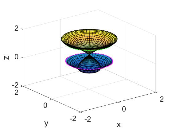
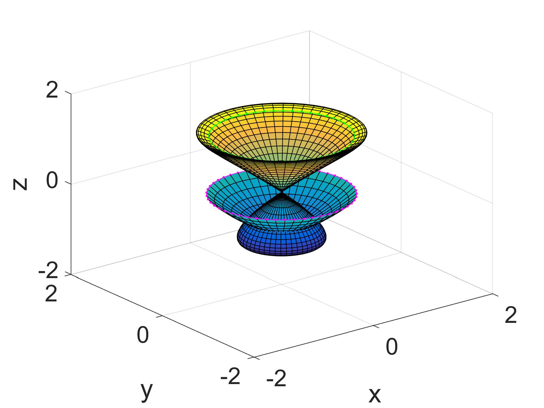
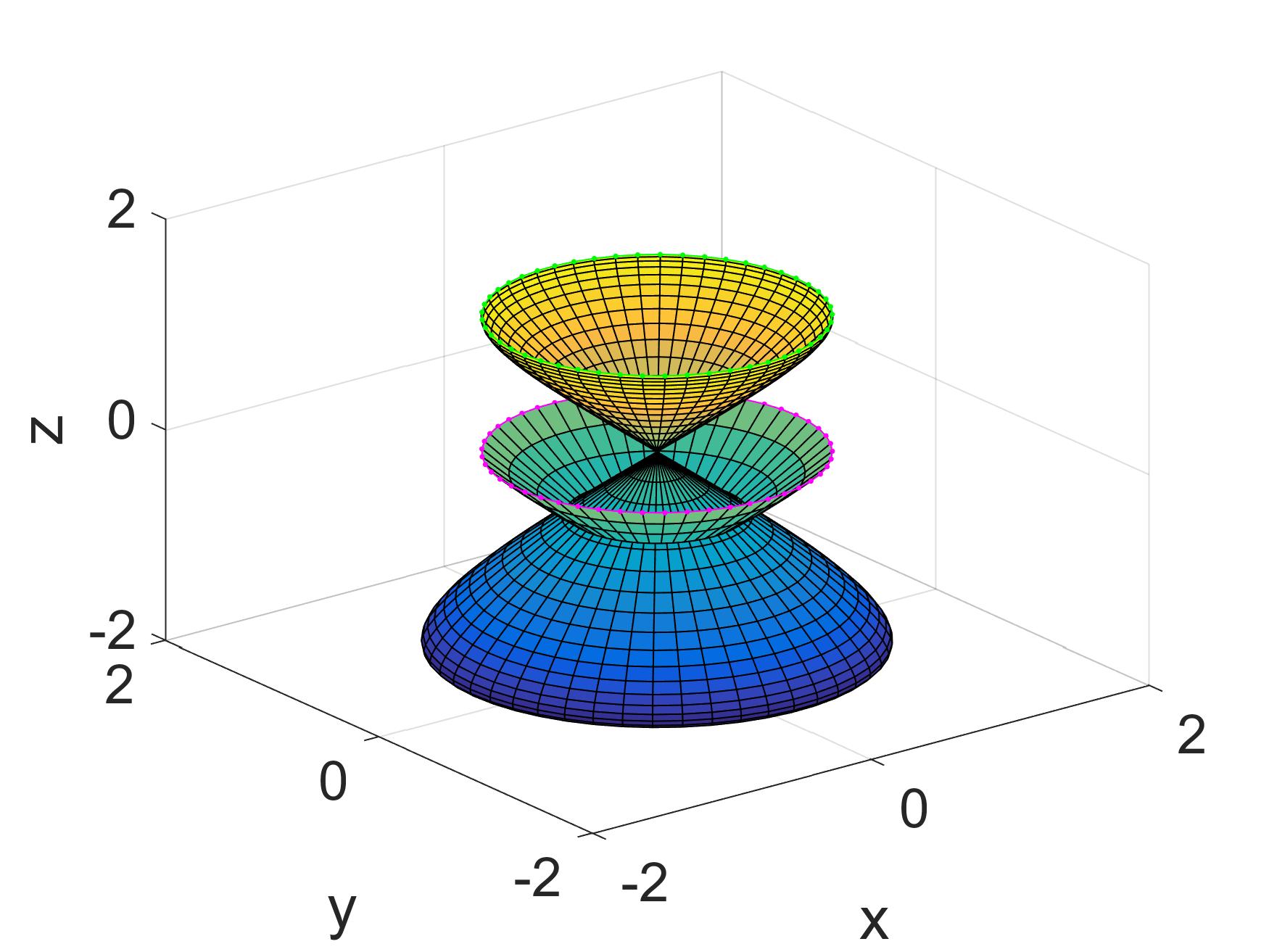
Figure 2: The adaptive formation change process of the multi-agent system with unknown delay initial value $\hat{D}(0)=4$. (a) $t=0s$ (b) $t=0.09s$ (c) $t=0.2s$ (d) $t=2s$ (e) $t=4s$ (f) $t=40s$.

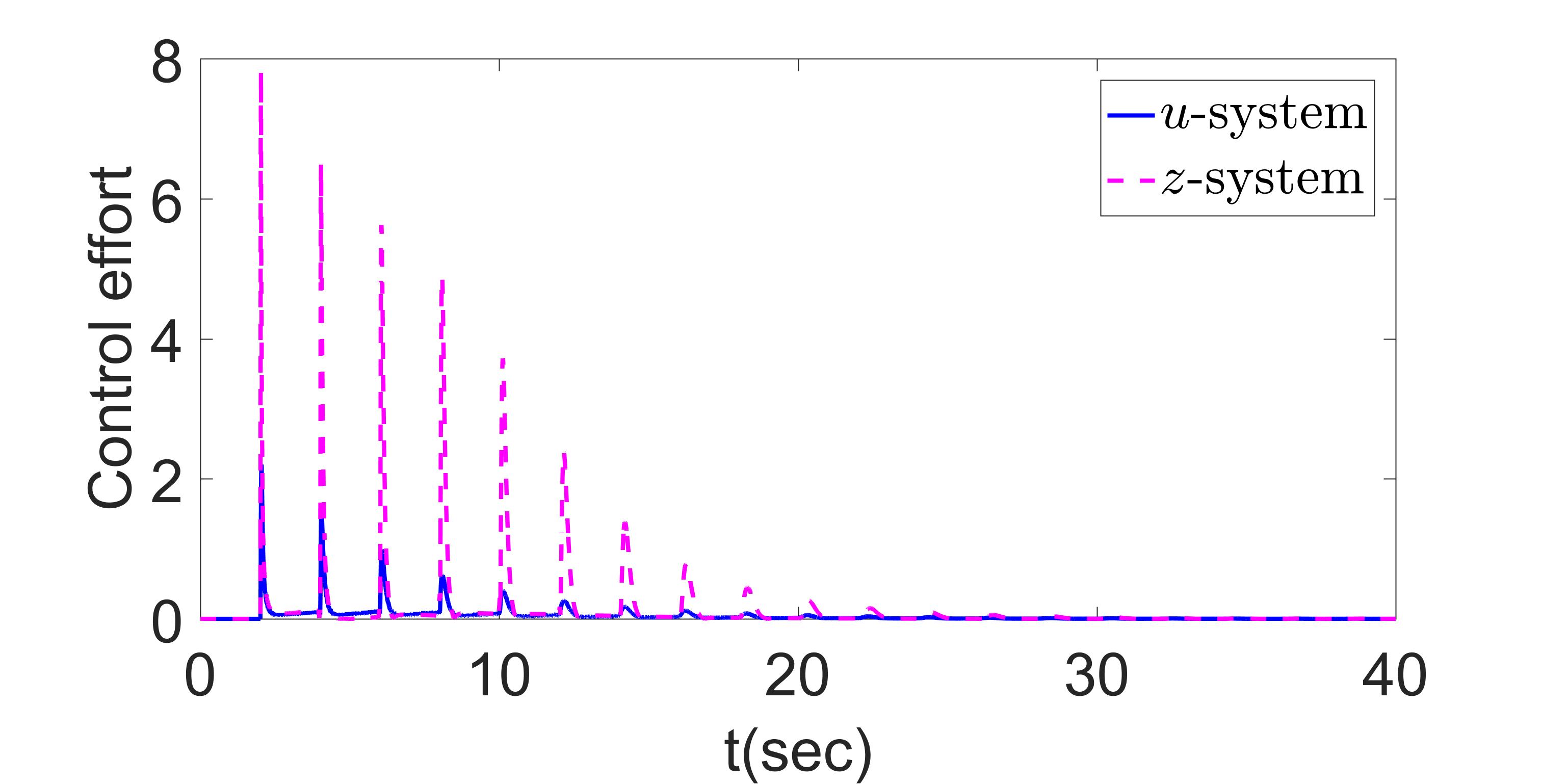
Figure 3: Time-evolution of the control signals

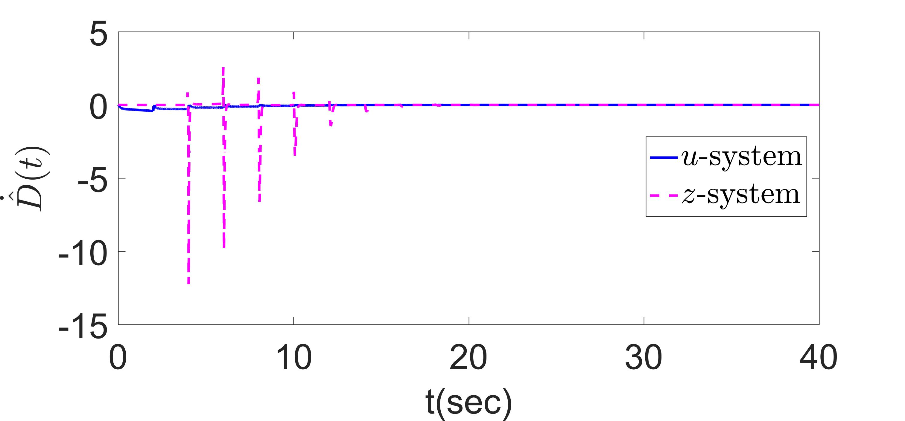
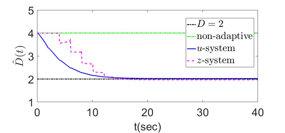
Figure 4: Delay estimate. (a) Dynamics of the updated law $\dot{\hat{D}}(t)$ (b) Time-evolution of the estimate of the unknown parameter $\hat{D}(t)$.

In Figure 5, (a) and (b) show the tracking error of agents indexed by $i=5$, $i=15$, $i=30$, and $i=51$ (actuator leaders) and the average of all agents on the horizontal and vertical directions, respectively, under non-adaptive boundary control. It can be seen from the figure that the tracking error gradually tends to $0$ with time evolution. Figures (c) and (d) show the $L^{2}$-norm of average tracking error of all the agents in the horizontal and vertical directions, respectively. It can be seen that if the estimate of unknown delay $\hat{D}$ does not match the true value of the delay $D=2$, namely if a delay mismatch occurs, the tracking error diverges.

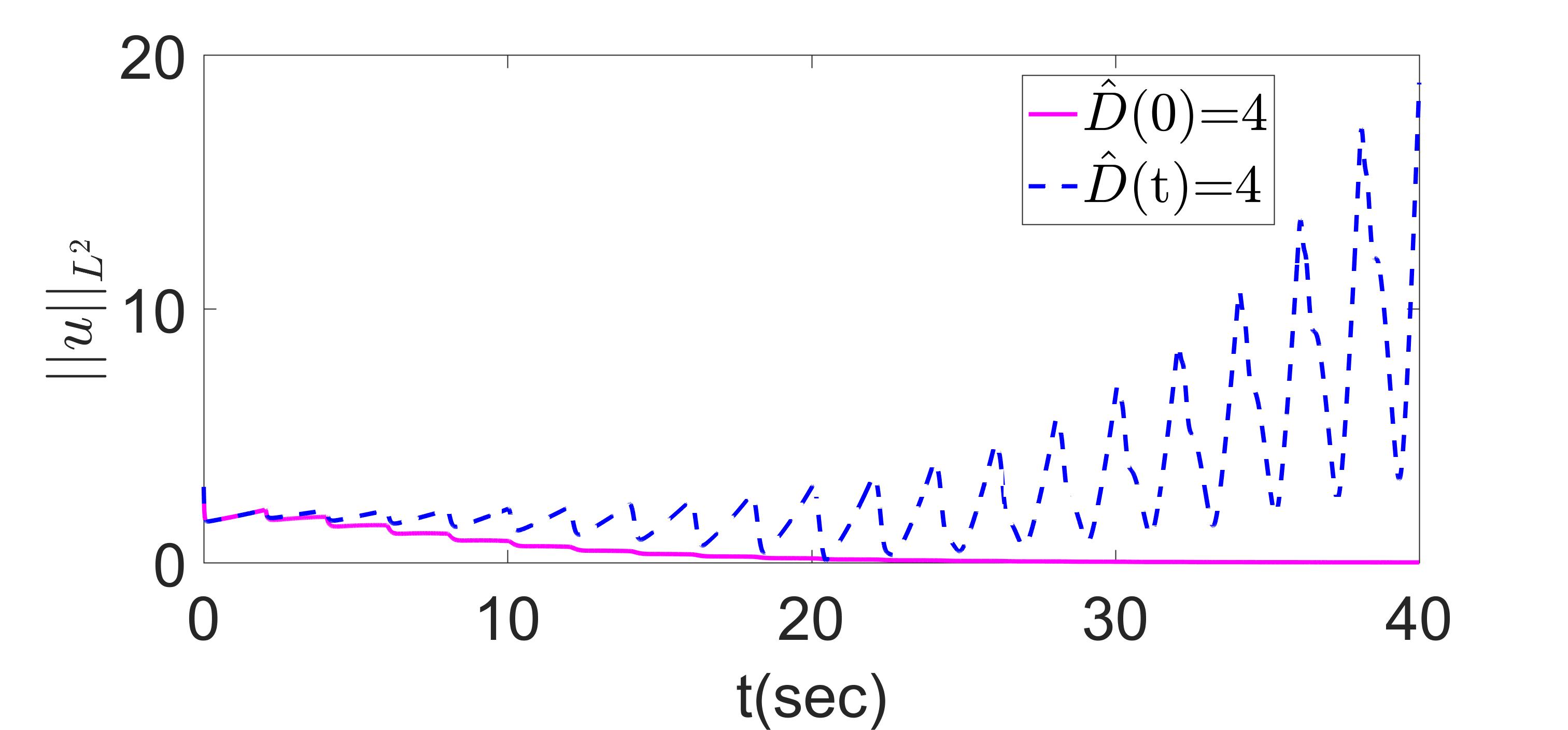
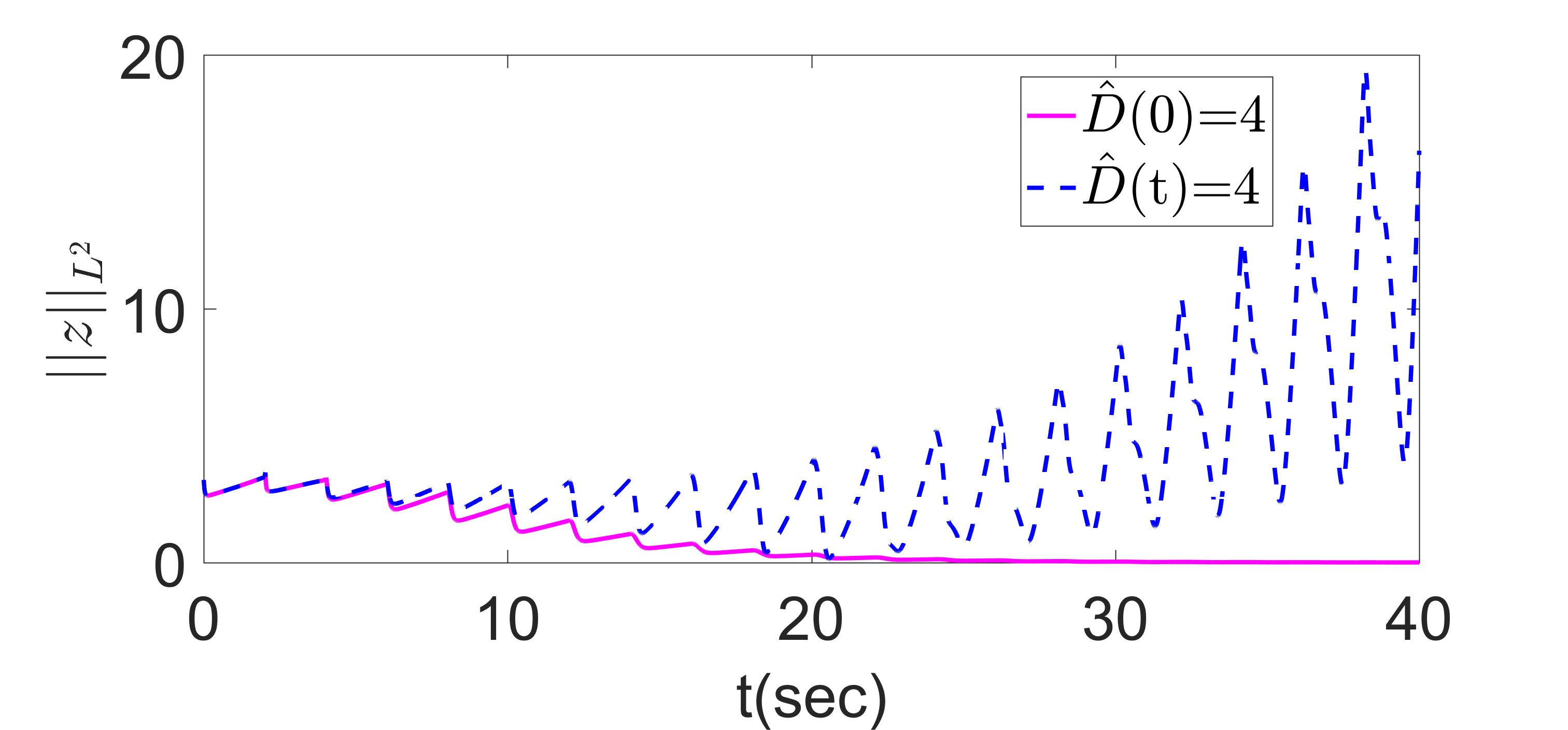
Figure 5: (a) Tracking error of $u$ system under adaptive control, (b) Observation error of $z$ system under adaptive control, (c) Average tracking error of $u$ system, (d) Average tracking error of $z$ system.

7 Conclusion

This paper studies the formation control of MAS with unknown input delay in 3D space via cylindrical topology. To accomplish the desired 3D formation with stable transitions, we propose an adaptive controller with the backstepping method. The update law for estimating the unknown parameter is established using the Lyapunov method. As the dimensionality increases, the complexity of the problem grows significantly. To address this, we introduce a Fourier series to transform the PDE describing the two-dimensional cylindrical communication topology into the sum of infinite one-dimensional systems. Subsequently, we prove the local stability of the closed-loop system and the regulation of the states to zero by a rather intricate Lyapunov function. In future work, we will extend our research to the systems subject to both unknown plant coefficients and input delays.

Appendix A The Proof of Proposition 1

To prove the norm equivalence between the state of the error system (13)–(17) and that of the target system (79)–(82), $S_{i}$, $i=1,2$ are constructed using the bound of the integral of kernels, for example, let’s consider the $L^{2}$ norm of $\vartheta(s,\theta,t)$. From equation (52), we get the following estimate

$$\int_{0}^{1}\int_{\pi}^{\pi}|{\vartheta}(s,\theta,t)|^{2}\mathrm{d}\theta\mathrm{d}s$$

$$\leq 3\rVert h\rVert^{2}+3\int_{0}^{1}\int_{-\pi}^{\pi}\bigg{(}\int_{0}^{1}\int_{-\pi}^{\pi}\eta(s,\tau,\theta,\psi,\hat{D})w(\tau,{\theta},t)$$

$$\mathrm{d}\psi\mathrm{d}\tau\bigg{)}^{2}\mathrm{d}\theta\mathrm{d}s+3\hat{D}^{2}\int_{0}^{1}\int_{-\pi}^{\pi}\bigg{(}\int_{0}^{s}\int_{-\pi}^{\pi}q(s,\tau,\theta,\psi,$$

$$\hat{D})h(\tau,{\theta},t)\mathrm{d}\psi\mathrm{d}\tau\bigg{)}^{2}\mathrm{d}\theta\mathrm{d}s.$$ (127)

From (54) and (55), we have

$$\eta(s,\tau,\theta,\psi,\hat{D})={Q(s,\theta-\psi,\hat{D})}F(s,\tau),$$ (128)

$$q(s,\tau,\theta,\psi,\hat{D})={Q(s-\tau,\theta-\psi,\hat{D})}G(s,\tau),$$ (129)

where

$$F(s,\tau) =2\sum_{i=1}^{\infty}e^{-\hat{D}i^{2}\pi^{2}s}\mathrm{sin}(i\pi\tau)\int_{0}^{1}\mathrm{sin}(i\pi\xi)l(1,\xi)\mathrm{d}\xi,$$ (130)

$$G(s,\tau) =-2\sum_{i=1}^{\infty}e^{-\hat{D}i^{2}\pi^{2}(s-\tau)}i\pi(-1)^{n}\int_{0}^{1}\mathrm{sin}(i\pi\xi)l(1,\xi)\mathrm{d}\xi.$$ (131)

For the second term on the left of the inequality (A), using Fourier series, the following relations hold (see (20))

$$w(s,\theta,t) =\sum_{n=-\infty}^{\infty}w_{n}(s,t)e^{\mathrm{j}n\theta},$$ (132)

and

$${Q(s,\theta-\psi,\hat{D})} =\frac{1}{2\pi}\sum_{n=-\infty}^{\infty}e^{-\hat{D}n^{2}s}e^{\mathrm{j}n(\theta-\psi)}.$$ (133)

It follows that

$$\int_{-\pi}^{\pi}Q(s,\theta-\psi,\hat{D})w(\tau,{\psi},t)\mathrm{d}\psi$$

$$=\frac{1}{2\pi}\sum_{n=-\infty}^{\infty}\sum_{m=-\infty}^{\infty}e^{-\hat{D}n^{2}s}w_{m}(\tau,t)\int_{-\pi}^{\pi}e^{\mathrm{j}n(\theta-\psi)}e^{\mathrm{j}m\psi}\mathrm{d}\psi$$

$$=\sum_{n=-\infty}^{\infty}e^{-\hat{D}n^{2}s}e^{\mathrm{j}n\theta}w_{n}(\tau,t),$$ (134)

where we have used the orthogonality property of the Fourier series (the same conclusion is reached using the convolution theorem). From the Parseval’s theorem, the following can be deduced

$$\int_{-\pi}^{\pi}\bigg{(}\int_{-\pi}^{\pi}Q(s,\theta-\psi,\hat{D})w(\tau,{\psi},t)\mathrm{d}\psi F(s,\tau)\bigg{)}^{2}\mathrm{d}\theta$$

$$=2\pi\sum_{n=-\infty}^{\infty}e^{-2\hat{D}n^{2}s}|w_{n}(\tau,t)|^{2}|F(s,\tau)|^{2}$$

$${\leq 2\pi\sum_{n=-\infty}^{\infty}|w_{n}(\tau,t)|^{2}|F(s,\tau)|^{2},}$$ (135)

which allow to state that

$$\int_{0}^{1}\int_{-\pi}^{\pi}\bigg{(}\int_{0}^{1}\int_{-\pi}^{\pi}Q(s,\theta-\psi,\hat{D})F(s,\tau)$$

$$\cdot w(\tau,{\psi},t)\mathrm{d}\psi\mathrm{d}\tau\bigg{)}^{2}\mathrm{d}\theta\mathrm{d}s$$

$$\leq\int_{0}^{1}\bigg{(}\int_{-\pi}^{\pi}\int_{0}^{1}\bigg{(}\int_{-\pi}^{\pi}Q(s,\theta-\psi,\hat{D})w(\tau,{\psi},t)\mathrm{d}\psi\bigg{)}^{2}\mathrm{d}\tau\mathrm{d}\theta$$

$$\cdot\int_{0}^{1}|F(s,\tau)|^{2}\mathrm{d}\tau\bigg{)}\mathrm{d}s$$

$$\leq\int_{0}^{1}\int_{0}^{1}\int_{-\pi}^{\pi}\bigg{(}\int_{-\pi}^{\pi}Q(s,\theta-\psi,\hat{D})w(\tau,{\psi},t)\mathrm{d}\psi\bigg{)}^{2}\mathrm{d}\tau\mathrm{d}\theta\mathrm{d}s$$

$$\cdot\int_{0}^{1}\int_{0}^{1}|F(s,\tau)|^{2}\mathrm{d}\tau\mathrm{d}s$$

$$\leq{2\pi}\int_{0}^{1}\sum_{n=-\infty}^{\infty}|w_{n}(\tau,t)|^{2}\mathrm{d}\tau\int_{0}^{1}\int_{0}^{1}|F(s,\tau)|^{2}\mathrm{d}\tau\mathrm{d}s$$

$$=\int_{0}^{1}\int_{0}^{1}|F(s,\tau)|^{2}\mathrm{d}\tau\mathrm{d}s\rVert w\rVert^{2}.$$ (136)

Similarly, for the third term on the left of the inequality (A), based on (133), (132) and the orthogonality property of Fourier series, one can get

$$\int_{-\pi}^{\pi}Q(s-\tau,\theta-\psi,\hat{D})h(\tau,{\psi},t)\mathrm{d}\psi$$

$$=\sum_{n=-\infty}^{\infty}e^{-\hat{D}n^{2}(s-\tau)}e^{\mathrm{j}n\theta}h_{n}(\tau,t).$$ (137)

From the Parseval’s theorem, the following can be deduced

$$\int_{-\pi}^{\pi}\bigg{(}\int_{-\pi}^{\pi}Q(s-\tau,\theta-\psi,\hat{D})G(s,\tau)h(\tau,{\psi},t)\mathrm{d}\psi\bigg{)}^{2}\mathrm{d}\theta$$

$$=2\pi\sum_{n=-\infty}^{\infty}e^{-2\hat{D}n^{2}(s-\tau)}|h_{n}(\tau,t)|^{2}|G(s,\tau)|^{2}$$

$${\leq 2\pi\sum_{n=-\infty}^{\infty}|h_{n}(\tau,t)|^{2}|G(s,\tau)|^{2},}$$ (138)

and consequently

$$\int_{0}^{1}\int_{-\pi}^{\pi}\bigg{(}\int_{0}^{s}\int_{-\pi}^{\pi}Q(s-\tau,\theta-\psi,\hat{D})G(s,\tau)$$

$$\cdot h(\tau,{\psi},t)\mathrm{d}\psi\mathrm{d}\tau\bigg{)}^{2}\mathrm{d}\theta\mathrm{d}s$$

$$\leq\int_{0}^{1}\int_{0}^{s}\int_{-\pi}^{\pi}\bigg{(}\int_{-\pi}^{\pi}Q(s-\tau,\theta-\psi,\hat{D})$$

$$\cdot h(\tau,{\psi},t)\mathrm{d}\psi\bigg{)}^{2}\mathrm{d}\tau\mathrm{d}\theta\mathrm{d}s\int_{0}^{1}\int_{0}^{s}|G(s,\tau)|^{2}\mathrm{d}\tau\mathrm{d}s$$

$$\leq{2\pi}\int_{0}^{1}\sum_{n=-\infty}^{\infty}|h_{n}(\tau,t)|^{2}\mathrm{d}\tau\int_{0}^{1}\int_{0}^{s}|G(s,\tau)|^{2}\mathrm{d}\tau\mathrm{d}s$$

$$\leq\int_{0}^{1}\int_{0}^{s}|G(s,\tau)|^{2}\mathrm{d}\tau\mathrm{d}s\rVert h\rVert^{2}.$$ (139)

Thus, combining with (136) and (139), we get

$$\int_{0}^{1}\int_{\pi}^{\pi}|{\vartheta}(s,\theta,t)|^{2}\mathrm{d}\theta\mathrm{d}s\leq 3\rVert h\rVert^{2}$$

$$+3\int_{0}^{1}\int_{-\pi}^{\pi}\bigg{(}\int_{0}^{1}\int_{-\pi}^{\pi}{Q(s,\theta-\psi,\hat{D})}F(s,\tau)w(\tau,{\theta},t)$$

$$\mathrm{d}\psi\mathrm{d}\tau\bigg{)}^{2}\mathrm{d}\theta\mathrm{d}s+3\hat{D}^{2}\int_{0}^{1}\int_{-\pi}^{\pi}\bigg{(}\int_{0}^{s}\int_{-\pi}^{\pi}{Q(s-\tau,\theta-\psi,\hat{D})}$$

$$\cdot G(s,\tau)h(\tau,{\theta},t)\mathrm{d}\psi\mathrm{d}\tau\bigg{)}^{2}\mathrm{d}\theta\mathrm{d}s$$

$$\leq 3(1+\overline{D}^{2})\int_{0}^{1}\int_{0}^{s}|G(s,\tau)|^{2}\mathrm{d}\tau\mathrm{d}s\rVert h\rVert^{2}$$

$$+3\int_{0}^{1}\int_{0}^{1}|F(s,\tau)|^{2}\mathrm{d}\tau\mathrm{d}s\rVert w\rVert^{2},$$ (140)

where $\int_{0}^{1}\int_{0}^{s}|G(s,\tau)|^{2}\mathrm{d}\tau\mathrm{d}s$ and $\int_{0}^{1}\int_{0}^{1}|F(s,\tau)|^{2}\mathrm{d}\tau\mathrm{d}s$ are bounded as established in [28], which complete the proof of Proposition 1.

References

• [1] X. Ai and L. Wang. Distributed fixed-time event-triggered consensus of linear multi-agent systems with input delay. International Journal of Robust and Nonlinear Control, 31(7):2526–2545, 2021.
• [2] J. Alonso-Mora, E. Montijano, T. Nägeli, O. Hilliges, M. Schwager, and D. Rus. Distributed multi-robot formation control in dynamic environments. Autonomous Robots, 43(5):1079–1100, 2019.
• [3] J. Alonso-Mora, T. Naegeli, P. Beardsley, and P. Beardsley. Collision avoidance for aerial vehicles in multi-agent scenarios. Autonomous Robots, 39(1):101–121, 2015.
• [4] J. W. Brown and R. V. Churchill. Complex variables and applications. Brown and Churchill series. McGraw-Hill Higher Education, 2009.
• [5] J. A. Fax and R. M. Murray. Information flow and cooperative control of vehicle formations. IEEE Transactions on Automatic Control, 49(9):1465–1476, 2004.
• [6] G. Ferrari-Trecate, A. Buffa, and M. Gati. Analysis of coordination in multi-agent systems through partial difference equations. IEEE Transactions on Automatic Control, 51(6):1058–1063, 2006.
• [7] G. Freudenthaler and T. Meurer. PDE-based multi-agent formation control using flatness and backstepping: Analysis, design and robot experiments. Automatica, 115:108897, 2020.
• [8] P. Frihauf and M. Krstic. Leader-enabled deployment onto planar curves: A PDE-based approach. IEEE Transactions on Automatic Control, 56(8):1791–1806, 2011.
• [9] W. Hou, M. Fu, H. Zhang, and Z. Wu. Consensus conditions for general second-order multi-agent systems with communication delay. Automatica, 75:293–298, 2017.
• [10] I. Karafyllis, M. Kontorinaki, and M. Krstic. Adaptive control by regulation-triggered batch least squares. IEEE Transactions on Automatic Control, 65(7):2842–2855, 2019.
• [11] M. Krstic. Control of an unstable reaction-diffusion PDE with long input delay. Systems & Control Letters, 58(10):773–782, 2009.
• [12] D. Lee and M. W. Spong. Agreement with non-uniform information delays. In American Control Conference (ACC), pages 756–761, 2006.
• [13] K. Li, C. Hua, X. You, and X. Guan. Distributed output-feedback consensus control for nonlinear multiagent systems subject to unknown input delays. IEEE Transactions on Cybernetics, 52(2):1292–1301, 2022.
• [14] P. Lin and W. Ren. Constrained consensus in unbalanced networks with communication delays. IEEE Transactions on Automatic Control, 59(3):775–781, 2014.
• [15] Z. Liu, D. Nojavanzadeh, D. Saberi, A. Saberi, and A. A. Stoorvogel. Scale-free protocol design for regulated state synchronization of homogeneous multi-agent systems with unknown and non-uniform input delays. Systems & Control Letters, 152:104927, 2021.
• [16] T. Meurer and M. Krstic. Finite-time multi-agent deployment: A nonlinear PDE motion planning approach. Automatica, 47(11):2534–2542, 2011.
• [17] J. Qi, R. Vazquez, and M. Krstic. Multi-agent deployment in 3-D via PDE control. IEEE Transactions on Automatic Control, 60(4):891–906, 2015.
• [18] J. Qi, S. Wang, J. Fang, and M. Diagne. Control of multi-agent systems with input delay via PDE-based method. Automatica, 106:91–100, 2019.
• [19] J. Qi, J. Zhang, and Y. Ding. Wave equation-based time-varying formation control of multiagent systems. IEEE Transactions on Control Systems Technology, 26(5):1578–1591, 2018.
• [20] A. Smyshlyaev and M. Krstic. Adaptive Control of Parabolic PDEs. Princeton University Press, 2010.
• [21] X. Tan, J. Cao, X. Li, and A. Alsaedi. Leader-following mean square consensus of stochastic multi-agent systems with input delay via event-triggered control. IET Control Theory & Applications, 12(2):299–309, 2017.
• [22] S. Tang, J. Qi, and J. Zhang. Formation tracking control for multi-agent systems: A wave-equation based approach. International Journal of Control, Automation and Systems, 15(6):2704–2713, 2017.
• [23] Y. Tian and C. Liu. Consensus of multi-agent systems with diverse input and communication delays. IEEE Transactions on Automatic Control, 53(9):2122–2128, 2008.
• [24] R. Vazquez and M. Krstic. Explicit output-feedback boundary control of reaction-diffusion PDEs on arbitrary-dimensional balls. ESAIM: Control, Optimisation and Calculus of Variations, 22(4):1078–1096, 2016.
• [25] H. Wang, D. Guo, X. Liang, W. Chen, G. Hu, and K. K. Leang. Adaptive vision-based leader-follower formation control of mobile robots. IEEE Transactions on Industrial Electronics, 64(4):2893–2902, 2017.
• [26] J. Wang and M. Diagne. Delay-adaptive boundary control of coupled hyperbolic PDE-ODE cascade systems. arXiv e-prints, pages arXiv–2301, 2023.
• [27] S. Wang, M. Diagne, and J. Qi. Delay-adaptive predictor feedback control of reaction–advection–diffusion PDEs with a delayed distributed input. IEEE Transactions on Automatic Control, 67(7):3762–3769, 2022.
• [28] S. Wang, J. Qi, and M. Diagne. Adaptive boundary control of reaction–diffusion PDEs with unknown input delay. Automatica, 134:109909, 2021.
• [29] S. Wang, J. Qi, and J. Fang. Control of 2-D reaction-advection-diffusion PDE with input delay. In 2017 Chinese Automation Congress (CAC), pages 7145–7150, 2017.
• [30] S. Wang, J. Qi, and M. Krstic. Delay-adaptive control of first-order hyperbolic PIDEs. arXiv preprint arXiv:2307.04212, 2023.
• [31] W. Yu, G. Chen, and M. Cao. Some necessary and sufficient conditions for second-order consensus in multi-agent dynamical systems. Automatica, 46(6):1089–1095, 2010.
• [32] P. Zetocha, L. Self, R. Wainwright, R. Burns, M. Brito, and D. Surka. Commanding and controlling satellite clusters. IEEE Intelligent Systems and their Applications, 15(6):8–13, 2000.
• [33] M. Zhang, A. Saberi, and A. A. Stoorvogel. Semi-global state synchronization for multi-agent systems subject to actuator saturation and unknown nonuniform input delay. IEEE Transactions on Network Science and Engineering, 8(1):488–497, 2021.
• [34] W. Zhu and Z. Jiang. Event-based leader-following consensus of multi-agent systems with input time delay. IEEE Transactions on Automatic Control, 60(5):1362–1367, 2015.