NeuKron: Constant-Size Lossy Compression of Sparse
Reorderable Matrices and Tensors (Supplementary Document)

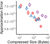
(a)

email

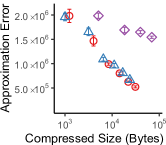
(b)

nyc

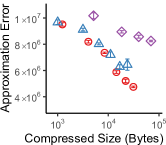
(c)

tky

Figure 11. When equipped with NeuKron, LSTM leads to concise and accurate compression. NeuKron with LSTM and that with GRU show perform similarly, but NeuKron with the decoder layer of Transformer requires significantly more space for the same level of approximation error.

1. Analysis for the type of the sequential model (Related to Section 4.1)

We compared the performances of auto-regressive sequence models, when they are equipped with NeuKron. We varied the hidden dimesion $h$ of NeuKron from 5 to 30 for LSTM and GRU, and the model dimension $d_{model}$ from 8 to 32 for the decoder layer of Transformer. As seen in Figure 11, when equipped with NeuKron, LSTM and GRU performed similarly, outperforming the decoder layer of Transformer.

2. Analysis on inference time
(Related to Section 4.3)

We measure the inference time for $10^{6}$ elements randomly chosen from square matrices of which numbers of rows and cols vary from $2^{7}$ to $2^{16}$. We ran 5 experiments for each size and report the average of them. As expected from Theorem 1 of the main paper, the approximation of each entry by NeuKron is almost in $\Omega(\log{M})$ (see Figure 13).

(a)

email

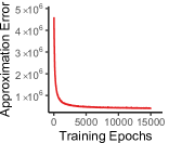
(b)

nyc

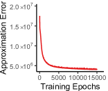
(c)

tky

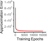
(d)

kasandr

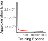
(e)

threads

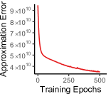
(f)

twitch

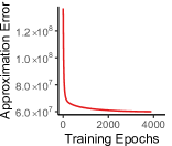
(g)

nips

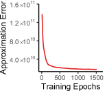
(h)

enron

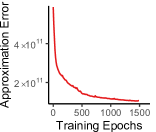
(i)

3-gram

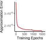
(j)

4-gram

Figure 12. Approximation error of NeuKron after each epoch. In most cases, the approximation error drops rapidly in early iterations, especially within one third of the total epochs that are determined by the termination condition in Section 6.1.

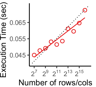
Figure 13. Inference time of NeuKron is nearly proportional to the logarithm of the number of rows and columns.

3. Analysis of the Tensor Extension
(Related to Section 5)

Below, we analyze the time and the space complexities of NeuKron extended to sparse reorderable tensors. For all proofs, we assume a $D$-order tensor $\mathcal{X}\in\mathbb{R}^{N_{1}\times\cdots\times N_{D}}$ where $N_{1}\leq N_{2}\leq\cdots\leq N_{D}$, without loss of generality. The complexities are the same with those in Section IV of the main paper if we assume a fixed-order tensor (i.e., if $D=O(1)$).

Theorem 1 (Approximation Time for Each Entry).

The approximation of each entry by NeuKron takes $\Theta(D\log N_{D})$ time.

Proof.

For encoding, NeuKron subdivides the input tensor $O(\log N_{D})$ times and each subdivision takes $O(D)$. For approximation, the length of the input of the LSTM equals to the number of the subdivisions, so the time complexity for retrieving each entry is $O(D\log N_{D})$. ∎

Theorem 2 (Training Time).

Each training epoch in NeuKron takes $O(\text{nnz}(\mathcal{X})\cdot D\log N_{D}+D^{2}N_{D})$.

Proof.

Since the time complexity for inference is $O(D\log N_{D})$ for each input, model optimization takes $O(\text{nnz}(\mathcal{X})\cdot D\log N_{D})$. For reordering, the time complexity of matching the indices as pairs for all the dimensions is bounded above to $O(D\cdot(DN_{D}))=O(D^{2}N_{D})$. For checking the criterion for all pairs, we need to retrieve all the non-zero entries, and it takes $O(\text{nnz}(\mathcal{X})\cdot D\log N_{D})$. Therefore, the overall training time per epoch is $O(\text{nnz}(\mathcal{X})\cdot D\log N_{D}+D^{2}N_{D})$. ∎

Theorem 3 (Space Complexity during Training).

NeuKron requires $O(D\cdot\text{nnz}(\mathcal{X})+D^{2}N_{D})$ space during training.

Proof.

The bottleneck is storing the input tensor in a sparse format, the random hash functions and the shingle values, which require $O(D\cdot\text{nnz}(\mathcal{X}))$, $O(\sum_{i=1}^{D}N_{i})$, and $O((D-1)\cdot\sum_{i=1}^{D}N_{i})$, respectively. Thus, the overall complexity during training is $O(D\cdot\text{nnz}(\mathcal{X})+(D-1)\cdot\sum_{i=1}^{D}N_{i})=O(D\cdot\text{nnz}(\mathcal{X})+D^{2}N_{D})$. ∎

Theorem 4 (Space Complexity of Outputs).

The number of model parameters of NeuKron is $\Theta(2^{D})$.

Proof.

In NeuKron, the number of parameters for LSTM does not depend on the order of the input tensor; thus, it is still in $\Theta(1)$. The embedding layer and the linear layers connected to the LSTM require $\Theta(2+2^{2}+\dots+2^{D})=\Theta(2^{D})$ parameters. ∎

4. Semantics and Properties of Datasets (Related to Section 6.1)

We provide the semantics of the datasets in Table 3 and the distributions of degrees, entry values, and connected-component sizes in Table 7. For degrees, we computed the sums of the rows and those of the columns for matrices. For connected-component sizes, we treated sparse matrices as bipartite graphs and used the number of nodes in each connected component as its size. Note that these properties are naturally extended to the tensors.

5. Implementation Details
(Related to Section 6.1)

We implemented NeuKron in PyTorch. We implemented the extended version of KronFit in C++. For ACCAMS, bACCAMS, and CMD, we used the open-source implementations provided by the authors. We used the svds function of SciPy for T-SVD. We used the implementations of CP and Tucker decompositions in Tensor Toolbox (bader2008efficient) in MATLAB. Below, we provide the detailed hyperparameter setups of each competitor.

• KronFit: The maximum size of the seed matrix was set as follows - email: 32 $\times$ 161, nyc: 33 $\times$ 196, tky: 14 $\times$ 40, kasandr: 75 $\times$ 80, threads: 57 $\times$ 85, twitch: 30 $\times$ 63. We tested the performance of KronFit when $\gamma$ is 1 and 10, and fixed $\gamma$ to $10$ because it performs better when $\gamma$ is set to 10. We performed a grid search for the learning rate in $\{10^{-1},10^{-2},\cdots,10^{-8}\}$.

• T-SVD: The ranks were up to 50 for email, 460 for nyc, 200 for tky, 15 for kasandr, 90 for threads, and 50 for twitch.

• CUR: We selected ranks for CUR from {10, 100, 1000}. We sampled {1%, 1.25%, 2.5%, 5%, 10%} of rows and columns in email , {3.3%, 5%, 10%, 14.3%, 20%} of rows and columns in nyc , and {1%, 2%, 4%, 8.3%, 11.1%} of rows and columns in tky

• CMD: We sampled (# rows, # columns) as much as {(30, 150), (60, 350), (90, 700), (100, 1400), (150, 2500)} for email, {(65, 2125), (125, 4250), (250, 8500), (500, 17000), (1000, 34000)} for nyc, {(45, 1315), (90, 2625), (175, 5250), (350, 10500), (700, 21000)} for tky, and {(55, 184), (109, 368), (218, 736), (436, 1471), (871, 2941)} for threads .

• ACCAMS: We used 5, 50, and 50 stencils for email, nyc, and tky, respectively. We used up to 48, 64, and 40 clusters of rows and columns for the aforementioned datasets, respectively.

• bACCAMS: We set the maximum number of clusters of rows and columns to 48, 48, and 24 for email, nyc, and tky, respectively. We used 50 stencils for the datasets.

• CP: The ranks were set up to 40 for nips, 8 for enron, 20 for 3-gram, and 4 for 4-gram.

• Tucker: We used hypercubes as core tensors. The maximum dimension of a hypercube for each dataset is as follows - nips: 40, enron: 6, 3-gram: 20, and 4-gram: 4.

Table 3. Semantics of Real-world Datasets

Name	Description
email	e-mail addresses $\times$ e-mails [binary]
nyc	venues $\times$ users [check-in counts]
tky	venues $\times$ users [check-in counts]
kasandr	offers $\times$ users [clicks]
threads	users $\times$ threads [participation]
twitch	streamers $\times$ users [watching time]
nips	papers $\times$ authors $\times$ words [counts]
4-gram	words $\times$ words $\times$ words $\times$ words [counts]
3-gram	words $\times$ words $\times$ words [counts]
enron	receivers $\times$ senders $\times$ words [counts]

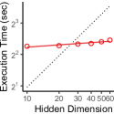
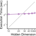
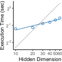
(a) threads

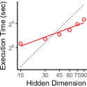
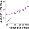
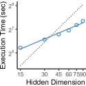
(b) twitch

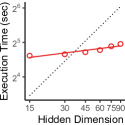
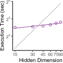
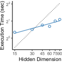
(c) 4-gram

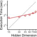
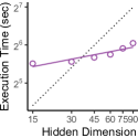
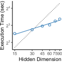
(d) enron

Figure 14. The training time of NeuKron is empirically sub-linear in the hidden dimension $h$ of NeuKron. We measure the total elapsed time, the elapsed time for order optimization, and the elapsed time for model optimization.

We followed the default setting in the official code from the authors for the other hyperparameters of ACCAMS and bACCAMS. The implementations of KronFit, T-SVD, CP, and Tucker used $8$ bytes for real numbers. The implementations of ACCAMS and bACCAMS used $4$ bytes for real numbers and assumed the Huffman coding for clustering results.

6. Hyperparameter analysis
(Related to Section 6.1)

We investigate how the approximation error of NeuKron varies depending on $\gamma$ values. We considered three $\gamma$ values and four datasets (email, nyc, tky, and kasandr) and reported the approximation error in Table 4. Note that setting $\gamma$ to $\infty$ results in a hill climbing algorithm that switches rows/column in pairs only if the approximation error decreases. The results show that, empirically, the approximation error was smallest when $\gamma$ was set to 10 on all datasets except for the nyc dataset.

Table 4. The effect of $\gamma$ on approximation error. We report the means and standard errors of approximation errors on the email, nyc, tky, and kasandr datasets.

Dataset	$\gamma$	Approximation error
email	1	90561.25 $\pm$ 467.996
	10	58691.88 $\pm$ 335.143
	$\infty$	59113.75 $\pm$ 891.544
nyc	1	421451.2 $\pm$ 4842.068
	10	402673.6 $\pm$ 17291.959
	$\boldsymbol{\infty}$	397947.5 $\pm$ 2393.016
tky	1	4166292.3 $\pm$ 143013.605
	10	3981669.6 $\pm$ 91907.201
	$\infty$	4034389.1 $\pm$ 48117.964
kasandr	1	6315784.36 $\pm$ 140974.6535
	10	4300280.71 $\pm$ 488804.599
	$\infty$	4385800.32 $\pm$ 496004.629

Table 5. Comparison of lossy-compression methods for sparse matrices and tensors. $nnz(\mathcal{X})$: the number of non-zeros in a matrix/tensor $\mathcal{X}$. $D$: the order of the input tensor. $N$ & $M$: the numbers of rows and columns of the input matrix. $N_{\max}$: the maximum dimensionality (i.e., $N_{\max}=\max(N_{1},\cdots,N_{D}$). $R$: rank. $S_{c}$ & $S_{r}$: the numbers of sampled rows and columns. $h$: the hidden dimension of the model of NeuKron. $T$: the number of iterations of an inner loop. $k$: the number of clusters of rows and columns. $w$: the weight parameter for the criterion of switching. $\alpha,\beta$: parameters for the probability distributions of clusters. $E_{r},E_{c}$: the number of rows and columns of a seed matrix.

Methods	Training	Inference	Hyperparameters
	Complexity	Complexity
NeuKron	$O(h^{2}nnz(\mathcal{X})\log(M))$	$O(h^{2}\log(N_{\max}))$	$h$, $w$, optimizer, learning rate
T-SVD (eckart1936approximation; baglama2005augmented)	$O(nnz(\mathcal{X})R+R^{3})$	$O(R)$	$R$
CMD (sun2007less)	$O(nnz(\mathcal{X})+S_{c}^{3}+S_{c}S_{r})$	$O(S_{r})$	$S_{c},S_{r}$
CUR (drineas2006fast)	$O(nnz(\mathcal{X})+S_{c}^{3}+S_{c}^{2}S_{r})$	$O(S_{r})$	$S_{c},S_{r}$
ACCAMS (beutel2015accams)	$O(NM+nnz(\mathcal{X})Tk)$	$O(R)$	$k,R$
bACCAMS(beutel2015accams)	$O(T\{k(N+M)$	$O(R)$	$k,R,\alpha,\beta$
	$+nnz(\mathcal{X})+NM+k^{2}\})$
KronFit (leskovec2007scalable; leskovec2010kronecker)	$O(nnz(\mathcal{X})\log(M))$	$O(\log(N_{\max}))$	$E_{r},E_{c}$, optimizer, learning rate
CP(carroll1970analysis)	$O(nnz(\mathcal{X})DR)$	$O(DR)$	$R$
Tucker(tucker1966some)	$O(nnz(\mathcal{X})DR)$	$O(DR^{D})$	$R$

7. Speed and Scalability on hidden dimension (Related to Appendix A.1)

We report the average the training time per epoch of NeuKron in Table 6. The training time per epoch varied from less than 1 second to more than 9 minutes depending on the dataset. As seen in Figure 12, the training plots of all datasets dropped dramatically within one third of total epochs that were determined by the termination condition in Section 6.1. Thus, a model that worked well enough could be obtained before convergence.

We also analyzed the effect of the hidden dimension $h$ on the training time per epoch of NeuKron. As seen in Figure 14, both the elapsed time for order optimization and the elapsed for model optimization were empirically sublinear in the hidden dimension.

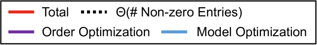
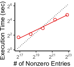
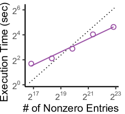
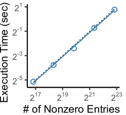
(a) 4-gram

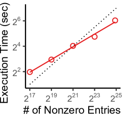
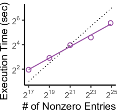
(b) enron

Figure 15. The training process of NeuKron on tensor is also scalable. Both model and order optimizations scale near-linearly with the number of non-zeros in the input.

8. Scalability on Tensor Datasets
(Related to Appendix A.1)

For the 4-gram and enron datasets, we generated multiple smaller tensors by sampling non-zero entries uniformly at random. The hidden dimension was fixed to $60$. Consistently with the results on matrices, the overall training process of NeuKron is also linearly scalable on sparse tensors, as seen in Figure 15.

Table 6. Training time per epoch on all datasets. We report the means and standard errors.

Dataset	Training time
(Hidden Dimension)
email (30)	0.19 $\pm$ 0.010
nyc (30)	0.21 $\pm$ 0.004
tky (30)	0.32 $\pm$ 0.005
kasandr (60)	1.93 $\pm$ 0.005
threads (60)	5.49 $\pm$ 0.012
twitch (90)	566.82 $\pm$ 3.308
nips (50)	6.31 $\pm$ 0.081
enron (90)	80.69 $\pm$ 0.266
3-gram (90)	27.19 $\pm$ 0.089
4-gram (90)	41.09 $\pm$ 0.785

Table 7. Structural properties of real-world datasets.

Dataset	Degrees				Entry Values	Connected Components
email
nyc
tky
kasandr
threads
twitch
nips
enron
3-gram
4-gram

9. Comparison of Lossy Compression Methods
(Related to Section 2)

In Table 5, we provide a comparison of lossy compression methods for sparase matrices and tensors, which supplement Table 1 in the main paper.