Nonanomalous heat transport in a one-dimensional composite chain.

Abstract

Translation-invariant low-dimensional systems are known to exhibit anomalous heat transport. However, there are systems, such as the coupled-rotor chain, where translation invariance is satisfied, yet transport remains diffusive. It has been argued that the restoration of normal diffusion occurs due to the impossibility of defining a global stretch variable with a meaningful dynamics. In this Letter, an alternative mechanism is proposed, namely, that the transition to anomalous heat transport can occur at a scale that, under certain circumstances, may diverge to infinity. To illustrate the mechanism, I consider the case of a composite chain that conserves local energy and momentum as well as global stretch, and at the same time obeys, in the continuum limit, Fourier’s law of heat transport. It is shown analytically that for vanishing elasticity the stationary temperature profile of the chain is linear; for finite elasticity, the same property holds in the continuum limit.

I Introduction

Heat transport in solids is described on a phenomenological level by Fourier’s law; the description fails, however, in low-dimensional systems, where heat transport takes an anomalous character such that the thermal conductivity of the material diverges with the sample size [1, 2, 3]. A standard method for the evaluation of thermal conductivity in solids is provided by the Green-Kubo formula [4] (see [2] for a simple derivation). In low dimensional systems, however, the heat current fluctuation correlation, on which the formula is based, diverges at large-scale, which prevents direct application of the method and suggests breakup of normal transport. Indeed, analysis of such divergences by renormalization techniques first allowed researchers to determine the anomalous scaling exponent for the thermal conductivity in low-dimensional systems [5] and implied that a coarse-grained description of the fluctuations in terms of field variables in a laboratory reference frame must take into account advection terms analogous to those in the Eulerian description of a fluid.

The analogy in the relation between Lagrangian and Eulerian description in a fluid, and the dynamics in the continuum limit, of a low-dimensional solid, was recognized in [6] and constitutes the basis for the derivation of the Nonlinear Fluctuating Hydrodynamic (NFH) theory [7]. The relevance of the fluid mechanic point of view in the description of heat transport in a low-dimensional solid is corroborated by the fact that the same anomalous behaviors are observed in one-dimensional particle models where the only interaction is provided by collisions, and which, at a coarse-grained level, can be described as bona fide one-dimensional fluids [8, 9].

The key mechanism leading to the divergence of the field equations, and hence to anomalous heat conduction in the systems under consideration, appears to be the simultaneous conservation locally of energy and momentum [10, 11, 5]. More recently, an additional condition has been identified in the fact that the global stretch of the system must have a dynamical content [12, 13]. If any such condition is violated—e.g. if the atoms in the chain interact with a substrate, leading to translation invariance violation, or if, as in the case of the coupled-rotor chain [14, 15], it is not possible to define a total stretch for the system—normal diffusion is recovered. In the same way, systems, such as the zero-range model [16] and the Kipnis-Presutti model [17] to name a few, in which energy is randomly exchanged between atoms without momentum conservation, are characterized by normal heat conduction.

To date, all analytical models of low-dimensional heat transport are based on mimicking the role of anharmonicity in spatially redistributing the vibration energy along the chain, by adding a stochastic component to the dynamics. The strategy to microscopically implement stochasticity is not unique. In [18], random collisions are assumed, with pairs of neighboring atoms exchanging momentum while their total energy remains constant. In other models, three-atom interactions are required to accommodate the joint conditions of energy and momentum conservation. In [19], the stochastic component of the dynamics is realized by a random walk in momentum space on the constant energy surface of the system. NFH predicts that for generic interaction potentials, the large-scale dynamics of energy and momentum preserving one-dimensional chains should fall in the universality class of the Kardar-Parisi-Zhang model [7]. There are special cases, however, in which the predictions of the NFH theory do not apply [7, 20], with finite-size effects, as well as weak chaos in the interaction, making the detection of universal behaviors difficult [21].

The situation as regards experiments and numerical (atomistic) simulation of more realistic systems is equally complicated. Results are indeed often dependent on the properties of the material and the experimental or numerical technique adopted (see [3] and references therein for an extended discussion). Of particular interest is the possible presence of a diffusive range at small scales, complicating the measurement of the anomalous scaling exponents predicted by the theory; such crossover behaviors are indeed predicted in particle systems [9].

The purpose of the present Letter is to study the crossover from small-scale thermal diffusion to large-scale anomalous heat conduction in the specific example of a “composite” chain, in which atoms interact with their neighbors through harmonic forces and inclusions acting as random sources and sinks of kinetic energy. Composite materials such as e.g. semiconductor perovskites find application in photovoltaics, and proper characterization of their thermal properties is particularly important [22]. The total momentum and energy of the atoms and the inclusion involved in an interaction are conserved, the ends of the chain are fixed, and thus all the conditions for anomalous heat conduction in the system are satisfied. Yet, the analysis that follows shows that the range in which heat transport is diffusive can greatly exceed the range in which the dynamics of the chain is viscous. In particular, heat transport becomes diffusive at all scales in the continuum limit.

II Outline of the model

The geometry of the system is illustrated in Fig. 1.

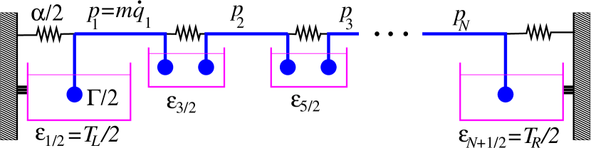
Figure 1: Sketch of the composite chain: the two-bead assemblies (blue online) represent the individual atoms; the cells underneath (magenta online) represent the zero-mass mobile inclusions and the thermal baths.

Each two-bead assembly represents an atom, with the bars joining the beads assumed rigid. The cells in the middle represent the inclusions, which for simplicity are taken to be massless; the cells at the extremes of the chain are the heat baths, whose position is fixed. Indicate with $N$ the number of atoms in the chain and with $L=N\eta$ the chain’s length. The inclusions act on the beads as Langevin baths with friction coefficient $\Gamma/2$ and noise amplitude

$$\langle\xi_{k+1/2}(0)\xi_{j+1/2}(t)\rangle=2m\Gamma\langle\epsilon\rangle_{k+1/2}\delta_{kj}\delta(t).$$ (1)

The adopted Langevin dynamics may be interpreted as the result of coarse graining the fast internal degrees of freedom in the inclusions, with $\epsilon_{k+1/2}$ an energy variable that is going to be determined dynamically from the condition of local energy conservation (see below).

The thermal baths at the chain extremes act on the respective atoms in the same way as the inclusions, with energy variables $\epsilon_{1/2}$ and $\epsilon_{N+1/2}$ replaced in Eq. (1) by fixed temperatures $T_{L}/2$ and $T_{R}/2$, $T_{L}-T_{R}=2\Delta T$ (the Boltzmann constant $k_{B}$ is set equal to 1 throughout the calculation).

Indicate with $q_{k}$ the displacement of the atoms from their equilibrium position and with $p_{k}=m\dot{q}_{k}$ the associated momentum. As illustrated in Fig. 1, the elastic force acts in parallel with that by the inclusion; the chain dynamics is then described by the system of equations, in the bulk $1<k<N$,

$$\dot{p}_{k} = \Gamma(p_{k+1}+p_{k-1}-2p_{k})/2$$ (2)

$$+ \alpha(q_{k+1}+q_{k-1}-2q_{k})/2+\xi_{k-1/2}-\xi_{k+1/2},$$

while at the ends of the chain,

$$\dot{p}_{1} = \Gamma(p_{2}-2p_{1})/2$$ (3)

$$+ \alpha(q_{2}-2q_{1})/2+\xi_{1/2}-\xi_{3/2},$$

$$\dot{p}_{N} = \Gamma(p_{N-1}-2p_{N})/2$$ (4)

$$+ \alpha(q_{N-1}-2q_{N})/2+\xi_{N-1/2}-\xi_{N+1/2}$$

(Itô’s prescription is assumed throughout the Letter). The conservative nature of the noise in Eqs. (2-4) should be noted, which distinguishes the present model from ones in which local heat baths force the dynamics, such as e.g. [24, 25].

It is possible to identify a microscopic elastic timescale $\omega_{\eta}^{-1}=\sqrt{m/\alpha}$, with the magnitude of the ratio

$$r=\omega_{\eta}/\Gamma$$ (5)

determining whether the microscopic dynamics is dominated by elasticity or by the effective friction generated by the inclusions. We can take the continuum limit of Eq. (2), and the result is :

$$\partial_{t}^{2}q = \partial_{x}^{2}(c_{s}^{2}+\nu\partial_{t})q+\partial_{x}\xi,$$ (6)

$$\langle\xi(x,t)\xi(0,0) = 2(\eta\langle\epsilon\rangle\nu/m)\delta(x)\delta(t),$$ (7)

which describes wave propagation in a viscoelastic (Kelvin-Voigt) medium with sound speed and viscosity, respectively,

$$c_{s}=\eta\omega_{\eta}\quad{\rm and}\quad\nu=\eta^{2}\Gamma.$$ (8)

From here, it is possible to define a viscous scale

$$l_{\nu}=\nu/c_{s}=\eta/r,$$ (9)

which identifies the upper limit of the viscosity-dominated range for the dynamics.

To study the fluctuation dynamics, one needs an equation for the energy variable $\epsilon_{k+1/2}$. One obtains such equation by imposing energy conservation in the interaction between atoms and inclusions. The energy budget in the interaction between atoms $k$ and $k+1$, and inclusion $k+1/2$ is obtained, for $1<k<N$, by evaluating the contribution to the variation of kinetic energy of the two atoms, $K_{k+1/2}=(p_{k+1}-p_{k})^{2}/(4m):=p_{k+1/2}^{2}/(4m)$, from the forcing by the inclusion. One can write in general

$$\dot{K}_{k+1/2}=-\dot{E}_{k+1/2}+\ldots,$$ (10)

where $E_{k+1/2}=E(\epsilon_{k+1/2})$ is the internal energy of the inclusion and the dots stand for the contributions from the elastic forces and the neighboring inclusions. Substituting Eq. (2) in the left hand side of Eq. (10) yields then

$$\dot{E}_{k+1/2} = 2\Gamma\Big{(}\frac{p^{2}_{k+1/2}}{4m}-\epsilon_{k+1/2}\Big{)}-\frac{p_{k+1/2}\xi_{k+1/2}}{m},$$ (11)

where one recognizes in the term $\Gamma p_{k+1/2}^{2}/(2m)$ the work by the friction forces, and in $2\Gamma\epsilon_{k+1/2}$ the average energy provided to the two atoms by the fluctuating force.

III The purely viscous chain

In the $\alpha\to 0$ limit, the system provides an example of heat transport by Brownian motion. Exactly as in the elastic case [27], it is possible to evaluate the heat flow from the dynamics of the one-time correlations . Define

$$\Pi_{ik}=\langle p_{i}p_{k}\rangle,\ Z_{ik}=\langle q_{i}p_{k}\rangle,\ Q_{ik}=\langle q_{i}q_{k}\rangle.$$ (12)

For $\alpha=0$, $q_{i}$ is an irrelevant variable, and the equation for $\Pi$ and those for $Z$ and $Q$ decouple. The last two variables can then, for the moment, be disregarded.

Let us focus first on the bulk; from Eq. (2), one obtains the equation for $\Pi_{ik}$

$$2\Gamma^{-1}\dot{\Pi}_{k,k+l} = \Pi_{k+1,k+l}+\Pi_{k-1,k+l}-2\Pi_{k,k+l}$$ (13)

$$+ \Pi_{k,k+1+l}+\Pi_{k,k-1+l}-2\Pi_{k,k+l}$$

$$+ 4m[(\delta_{l0}-\delta_{l1})\langle\epsilon\rangle_{k+1/2}$$

$$+ (\delta_{l0}-\delta_{l,-1})\langle\epsilon\rangle_{k-1/2}],$$

where $1<k,k+l<N$. At stationarity, one gets from Eq. (11)

$$4m\langle\epsilon\rangle_{k+1/2} = \langle p_{k+1/2}^{2}\rangle$$ (14)

$$= \Pi_{kk}+\Pi_{k+1,k+1}-2\Pi_{k,k+1},$$

which, substituted into Eq. (13), yields

$$-2\Pi_{kk}+\Pi_{k+1,k+1}+\Pi_{k-1,k-1} = 0,$$ (15)

$$-2\Pi_{k,k+1}+\Pi_{k,k+2}+\Pi_{k+1,k-1} = 0,$$ (16)

$$\Pi_{k+1,k+l}+\Pi_{k-1,k+l}+\Pi_{k,k+1+l}$$

$$\qquad+\Pi_{k,k-1+l}-4\Pi_{k,k+l} = 0,\quad|l|>1.$$ (17)

The same procedure can be carried out at $k=1$,

$$\Pi_{22}-3\Pi_{11}+2mT_{L} = 0,$$ (18)

$$\Pi_{13}-2\Pi_{12} = 0,$$ (19)

$$\Pi_{2l}-4\Pi_{1l}+\Pi_{1,l-1}+\Pi_{1,l+1} = 0,\quad l>2,$$ (20)

and a similar set of equations is produced at $k=N$. The system of equations (15-20) has the remarkable property that Eqs. (16,17,19,20), which involve out-of-diagonal terms, decouple from Eqs. (15) and (18) on the diagonal. Equations (15) and (18) tell us that $\Pi_{kk}$ has a linear profile:

$$2(mT_{L}-\Pi_{11})=\Pi_{kk}-\Pi_{k+1,k+1}$$

$$=2(\Pi_{NN}-mT_{R})=2m\Delta T/N.$$ (21)

On the other hand, Eqs. (16,17,19,20) admit the zero solution $\Pi_{kl}=0$, $k\neq l$, which is also necessarily unique, since a nonzero solution could have arbitrary amplitude and lead to negative $\langle(p_{l}+p_{k})^{2}\rangle$). From Eq. (21), it is then possible to write

$$\Pi_{kl}=m\Big{(}T_{L}+\frac{2k-1}{N}\Delta T\Big{)}\delta_{kl};$$ (22)

The temperature profile along the purely viscous chain, $T_{k}\equiv\Pi_{kk}/m\simeq 2\langle\epsilon_{k+1/2}\rangle$, is thus linear.

For $\alpha=0$, the heat transfer along the chain is mediated by the work on the atoms by the inclusions; the average work by inclusion $k-1/2$ on the atom to its right thus coincides with the heat flux at site $k$

$$J_{k} = \Gamma\Big{[}\langle\epsilon\rangle_{k-1/2}-\frac{\langle p_{k}(p_{k}-p_{k-1})\rangle}{2m}\Big{]},$$ (23)

where it is understood that $p_{0}=0$. At stationarity, from Eqs. (14) and (22),

$$\frac{J_{k}}{\Gamma}=\frac{T_{L}}{2}-\frac{\Pi_{11}}{2m}=\frac{\Pi_{k-1,k-1}-\Pi_{kk}}{4m}=\frac{\Pi_{NN}}{2m}-\frac{T_{R}}{2},$$

which, using again Eq. (22), implies Fourier’s law; after reinstating Boltzmann’s constant,

$$J=\kappa\frac{T_{L}-T_{R}}{L},\qquad\kappa=\frac{k_{B}\nu}{4\eta}.$$ (24)

Setting $T_{L}=T_{R}=T$, it is easy to verify from Eqs. (14), (23) and (22), that at equilibrium $J_{k}=0$ and equipartition holds: $\langle\epsilon\rangle_{k+1/2}=\Pi_{kk}/(2m)=T/2$.

IV The effect of finite elasticity

For finite $\alpha$, part of the heat transfer is mediated by the elastic forces, with a contribution to the heat flux [1]:

$$\delta J^{el}_{k}=\alpha(Z_{kk}-Z_{k+1,k})/(2m).$$ (25)

To evaluate $\delta J^{el}_{k}$, we need an equation for $Z_{ik}$. Indicate

$$A_{ik}=\Gamma Z_{ik}+\alpha Q_{ik}.$$ (26)

The stationarity conditions $\dot{Z}_{k,k+l}+\dot{Z}_{k+l,k}=0$ and $\dot{Z}_{k,k+l}-\dot{Z}_{k+l,k}=0$ take the form, in the bulk, from Eq. (2):

$$-4\Pi_{k+l,k}/m=A_{k+l,k+1}+A_{k+l,k-1}$$

$$-2A_{k+l,k}+A_{k,k+l+1}+A_{k,k+l-1}-2A_{k,k+l},$$ (27)

$$A_{k+l,k+1}+A_{k+l,k-1}-2A_{k+l,k}$$

$$=A_{k,k+l+1}+A_{k,k+l-1}-2A_{k,k+l}.$$ (28)

Equations (27) and (28) imply $-2\Pi_{k+l,k}/m=A_{k+l,k+1}+A_{k+l,k-1}-2A_{k+l,k}$, better rewritten as

$$\partial_{k}^{2}A_{lk}=-2\Pi_{lk}/m,\quad 1<k,l<N.$$ (29)

where $\partial_{k}$ indicates finite difference: $\partial_{k}^{2}f=f_{k+1}+f_{k-1}-2f_{k}$. Identify with a bar the zero-viscosity component of quantities and with a tilde the respective correction, $\Pi=\bar{\Pi}+\tilde{\Pi}$, and make the ansatz (to be verified a posteriori) that if the chain is sufficiently short viscosity will dominate thermal fluctuations. It is then possible to set in Eq. (29) $\Pi_{lk}\simeq\bar{\Pi}_{lk}=\bar{\Pi}_{ll}\delta_{lk}$ [see Eq. (22)], which yields the solution

$$A_{lk}\simeq a_{l}+b_{l}k-\bar{\Pi}_{ll}|k-l|/m.$$ (30)

To determine the coefficients $a_{l}$ and $b_{l}$, one needs boundary conditions, which are provided by imposing stationarity at the ends of the chain, $\dot{Z}_{1k}=\dot{Z}_{Nk}=0$; exploiting Eqs. (2), (3) and (4):

$$2\Pi_{l1}/m = 2A_{l1}-A_{l2},$$

$$2\Pi_{lN}/m = 2A_{lN}-A_{l,N-1},\quad 1<l<N.$$ (31)

From $\Pi_{1l}\simeq\Pi_{lN}\simeq 0$, $1<l<N$, the following relations are then obtained:

$$A_{l2}\simeq 2A_{l1},\quad A_{l,N-1}\simeq 2A_{lN},\quad 1<l<N.$$ (32)

Substituting Eq. (30) into Eq. (32) yields

$$a_{l}\simeq\frac{l\bar{\Pi}_{ll}}{m},\quad b_{l}\simeq\frac{\bar{\Pi}_{ll}}{m}\frac{N+1-2l}{N+1},\quad 1<l<N.$$ (33)

Exploiting Eq. (30) and the relation $\bar{\Pi}_{kk}-\bar{\Pi}_{k+1,k+1}=2m\Delta T/N$ [see Eq. (21)], we obtain the expression, valid for $1<l\leq k<N$,

$$Z_{lk} \simeq \frac{A_{lk}-A_{kl}}{2\Gamma}=\frac{l(N+1-k)(\bar{\Pi}_{ll}-\bar{\Pi}_{kk})}{m\Gamma(N+1)}$$ (34)

$$= \frac{2l(N+1-k)(l-k)\Delta T}{\Gamma N(N+1)}.$$

Substituting Eq. (34) into Eq. (25) finally yields

$$\delta J_{k}^{el}\simeq-\frac{\alpha(1+k)(N+1-k)\Delta T}{\Gamma mN(N+1)},$$ (35)

and hence, by comparing with Eq. (24), the estimate

$$\delta J^{el}/J\sim r^{2}N=\eta L/l_{\nu}^{2},$$ (36)

which tells us that as long as

$$L\ll l_{\kappa}=l^{2}_{\nu}/\eta,$$ (37)

heat transport remains diffusive. A similar estimate holds for the momentum fluctuation amplitude, $\tilde{\Pi}/\bar{\Pi}\sim r^{2}N$ (see Supplemental Material [30]), which confirms the ansatz at the basis of Eq. (30). Note that in the continuum limit $\eta\to 0$ (all macroscopic quantities $L$, $Nk_{B}T$, $Nm$, $\nu$ and $c_{s}$ fixed and finite), the diffusive scale $l_{\kappa}$ goes to infinity and Fourier’s law holds irrespective of the sample size.

An interesting question concerns the role of possible violations of stretch conservation in the regime $L\ll l_{\kappa}$. By construction, for finite $\alpha$, the total stretch $\delta L$ is controlled by elasticity, which means that, strictly speaking, the total stretch is conserved. One may nevertheless argue that if, for $l_{\nu}\ll L\ll l_{\kappa}$ (that is the range where the dynamics of the chain is elastic), the ratio $\delta L/L$ in the continuum limit were to diverge to infinity, the chain would be behaving as if its endpoints were unconstrained. In other words, diffusive transport for $l_{\nu}\ll L\ll l_{\kappa}$ could be the consequence of insufficient conservation of stretch. We show below that this is not the case.

The continuum limit $\eta\to 0$ ($L$, $Nk_{B}T$, $Nm$, $\nu$ and $c_{s}$ fixed and finite) corresponds to a regime $L\ll l_{\kappa}$ such that Eq. (22) applies. It is then possible to estimate for the stretch $\delta L\sim\sqrt{N\langle q_{k+1/2}^{2}\rangle}$, where $q_{k+1/2}=q_{k+1}-q_{k}$; for small deviations from equilibrium, $T_{L}\simeq T_{R}\sim T$, $\langle q_{k+1/2}^{2}\rangle\sim v_{th}^{2}m/\alpha=(v_{th}/\omega_{\eta})^{2}$, where $v_{th}=\sqrt{k_{B}T/m}$ is the thermal velocity, which remains finite in the limit. From Eqs. (8) and (9) one then gets

$$\frac{\delta L}{L}\sim\frac{N^{1/2}v_{th}}{L\omega_{\eta}}=\frac{N^{1/2}\eta v_{th}}{Lc_{s}}=\frac{\sqrt{l_{\nu}\eta}}{L}\frac{v_{th}}{c_{s}},$$ (38)

which tells us that the relative stretch vanishes in the continuum limit (all quantities in the right hand side of the formula remain finite, except $\eta$, which vanishes); this suggests that stretch conservation violations do not play a role in the dynamics under consideration. (An alternative derivation of the result is provided in the Supplemental Material [30].)

V Conclusion

The present analysis shows that heat transport in a composite chain with a purely viscous microscopic dynamics, obeys Fourier’s law. By construction, no internal forces are generated in response to stretching of the system, and we thus have another example, beside that of the coupled-rotor chain, of a system conserving local energy and momentum, in which global stretch is not conserved and heat transport is diffusive.

If elasticity is finite, but there is a viscous range extending to macroscopic scales, the range of scales where heat transport is diffusive greatly exceeds the viscous range, and extends to infinity in the continuum limit. This is the main result of the Letter. The global stretch fluctuations vanish in the limit, which means that diffusive heat transport in such composite chain, contrary to the case of the coupled-rotor chain, cannot be explained by non-conservation of the stretch.

Some questions remain open. Is anomalous heat transport in the composite chain recovered at scales larger than the diffusion length $l_{\kappa}$? Is the existence of an extended diffusive range a common property of viscoelastic one-dimensional chains? The answer is probably yes in both cases , but, to prove the statement, going beyond the present perturbative—model-dependent analysis, would be required.

SUPPLEMENTAL MATERIAL

A: Finite elasticity correction to the momentum fluctuation amplitude

An equation for the stationary momentum correlation in the bulk, valid for generic $\alpha$, can be obtained from Eqs. (2) and (11):

$$\partial_{k}^{2}\Pi_{kk}+(\alpha/\Gamma)(Z_{k+1,k}+Z_{k-1,k})=0.$$ (39)

By exploiting Eq. (34), Eq. (39) takes the form, valid for small $r$ and large $N$,

$$\partial_{k}^{2}\Pi_{kk}\simeq\frac{4\alpha\Delta T(N/2-k)}{\Gamma^{2}N^{2}}.$$ (40)

Equation (40) has the general solution

$$\Pi_{kk}\simeq\frac{8\alpha\Delta T}{3\Gamma^{2}N^{2}}(N/2-k)^{3}+c_{0}+c_{1}k.$$ (41)

The homogeneous part of the solution is fixed by the boundary conditions

$$\Pi_{11}=mT_{L},\qquad\Pi_{NN}=mT_{R}.$$ (42)

From Eq. (22) one obtains then the expression for the elastic correction

$$\tilde{\Pi}_{kk}=\Pi_{kk}-\bar{\Pi}_{kk}\simeq\frac{8\alpha\Delta T}{3\Gamma^{2}N^{2}}[(N/2-k)^{3}-N^{2}(N/2-k)/4].$$ (43)

and hence the estimate [see Eq. (36)]

$$\frac{\tilde{\Pi}_{kk}}{m\Delta T}\sim r^{2}N\sim\frac{\delta J^{el}_{k}}{J}.$$ (44)

B: Stretch fluctuation amplitude — alternative calculation.

The stretch fluctuation can be estimated as $\delta L\sim\langle q_{j}^{2}\rangle^{1/2}$, where $\langle q_{j}^{2}\rangle\equiv Q_{jj}$. By switching to Fourier space in both space and time, we easily obtain from Eqs. (6) and (7) the fluctuation spectrum

$$Q_{k\omega}=\frac{2\nu\epsilon k^{2}}{\rho[(\omega^{2}-c_{s}^{2}k^{2})^{2}+\nu^{2}k^{4}]}=\frac{\nu k_{B}Tk^{2}}{\rho[(\omega^{2}-c_{s}^{2}k^{2})^{2}+\nu^{2}k^{4}]},$$ (45)

where $\rho=m/\eta$ is the chain density and $k$ indicates here wavenumbers. The denominator of $Q_{k\omega}$ has roots

$$kl_{\nu}\gg 1:\qquad\omega_{1}\simeq\pm{\rm i}\nu k^{2},\quad\omega_{2}=\pm{\rm i}c_{s}^{2}/\nu,$$

$$kl_{\nu}\ll 1:\qquad\omega_{1}\simeq c_{s}k\pm{\rm i}\nu k^{2},\quad\omega_{2}=-c_{s}k\pm{\rm i}\nu k^{2};$$

we thus get for $kl_{\nu}\gg 1$

$$Q_{k}=\int\frac{{\rm d}\omega}{2\pi}\frac{\nu k_{B}Tk^{2}}{\rho(\omega^{2}+\nu^{2}k^{4})(\omega^{2}+c_{s}^{4}/\nu^{2})}=\frac{\nu k_{B}T}{2\rho c_{s}^{2}(c_{s}^{2}/\nu+\nu k^{2})}\simeq\frac{k_{B}T}{2\rho c_{s}^{2}k^{2}},$$ (46)

while for $kl_{\nu}\ll 1$ we have

$$Q_{k} = \int\frac{{\rm d}\omega}{2\pi}\frac{\nu k_{B}Tk^{2}}{\rho[(\omega-c_{s}k)^{2}+\nu^{2}k^{4}][(\omega+c_{s}k)^{2}+\nu^{2}k^{4}]}$$ (47)

$$= \frac{k_{B}T}{4\rho\nu(\nu^{2}k^{4}+c_{s}^{2}k^{2})}\simeq\frac{k_{B}T}{4\rho c_{s}^{2}k^{2}}.$$

From here we get the displacement fluctuation amplitude in a chain of length $L$

$$\langle q^{2}\rangle\sim\int_{kL>1}{\rm d}kQ_{k}\sim\frac{k_{B}TL}{\rho c_{s}^{2}}\sim(v_{th}/c_{s})^{2}\eta L,$$ (48)

and hence the estimate for the stretch, valid for both $l_{\nu}\ll L$ and $l_{\nu}\gg L$,

$$\delta L\sim\langle q^{2}\rangle^{1/2}\sim\frac{v_{th}\sqrt{\eta L}}{c_{s}}=\frac{v_{th}N^{1/2}\eta}{c_{s}}$$ (49)

[compare with Eq. (38)].

References

- Lepri et al. [2003] S. Lepri, R. Livi, and A. Politi, Thermal conduction in classical low-dimensional lattices, Physics reports 377, 1 (2003).
- Dhar [2008] A. Dhar, Heat transport in low-dimensional systems, Advances in Physics 57, 457 (2008).
- Benenti et al. [2022] G. Benenti, D. Donadio, S. Lepri, and R. Livi, Non-fourier heat transport in nanosystems, arXiv preprint arXiv:2212.09374 (2022).
- Kubo et al. [2012] R. Kubo, M. Toda, and N. Hashitsume, Statistical physics II: nonequilibrium statistical mechanics, Springer Series in Solid-State Sciences, Vol. 31 (Springer Science & Business Media, 2012).
- Narayan and Ramaswamy [2002] O. Narayan and S. Ramaswamy, Anomalous heat conduction in one-dimensional momentum-conserving systems, Physical Review Letters 89, 200601 (2002).
- Chetrite and Gawȩdzki [2009] R. Chetrite and K. Gawȩdzki, Eulerian and lagrangian pictures of non-equilibrium diffusions, Journal of Statistical Physics 137, 890 (2009).
- Spohn [2014a] H. Spohn, Nonlinear fluctuating hydrodynamics for anharmonic chains, Journal of Statistical Physics 154, 1191 (2014a).
- Kundu et al. [2016] A. Kundu, O. Hirschberg, and D. Mukamel, Long range correlations in stochastic transport with energy and momentum conservation, Journal of Statistical Mechanics: Theory and Experiment 2016, 033108 (2016).
- Miron et al. [2019] A. Miron, J. Cividini, A. Kundu, and D. Mukamel, Derivation of fluctuating hydrodynamics and crossover from diffusive to anomalous transport in a hard-particle gas, Physical Review E 99, 012124 (2019).
- Prosen and Campbell [2000] T. Prosen and D. K. Campbell, Momentum conservation implies anomalous energy transport in 1d classical lattices, Physical Review Letters 84, 2857 (2000).
- Bonetto et al. [2000] F. Bonetto, J. L. Lebowitz, and L. Rey-Bellet, Fourier’s law: a challenge to theorists, in Mathematical physics 2000 (World Scientific, 2000) pp. 128–150.
- Spohn [2014b] H. Spohn, Fluctuating hydrodynamics for a chain of nonlinearly coupled rotators, arXiv preprint arXiv:1411.3907 (2014b).
- Das and Dhar [2014] S. G. Das and A. Dhar, Role of conserved quantities in normal heat transport in one dimenison, arXiv preprint arXiv:1411.5247 (2014).
- Giardina et al. [2000] C. Giardina, R. Livi, A. Politi, and M. Vassalli, Finite thermal conductivity in 1d lattices, Physical Review Letters 84, 2144 (2000).
- Gendelman and Savin [2000] O. V. Gendelman and A. V. Savin, Normal heat conductivity of the one-dimensional lattice with periodic potential of nearest-neighbor interaction, Physical Review Letters 84, 2381 (2000).
- Evans and Hanney [2005] M. R. Evans and T. Hanney, Nonequilibrium statistical mechanics of the zero-range process and related models, Journal of Physics A: Mathematical and General 38, R195 (2005).
- Kipnis et al. [1982] C. Kipnis, C. Marchioro, and E. Presutti, Heat flow in an exactly solvable model, Journal of Statistical Physics 27, 65 (1982).
- Lepri et al. [2009] S. Lepri, C. Mejia-Monasterio, and A. Politi, A stochastic model of anomalous heat transport: analytical solution of the steady state, Journal of Physics A: Mathematical and Theoretical 42, 025001 (2009).
- Basile et al. [2006] G. Basile, C. Bernardin, and S. Olla, Momentum conserving model with anomalous thermal conductivity in low dimensional systems, Physical Review Letters 96, 204303 (2006).
- Lee-Dadswell [2015] G. R. Lee-Dadswell, Universality classes for thermal transport in one-dimensional oscillator systems, Physical Review E 91, 032102 (2015).
- Lepri et al. [2020] S. Lepri, R. Livi, and A. Politi, Too close to integrable: Crossover from normal to anomalous heat diffusion, Physical Review Letters 125, 040604 (2020).
- Caddeo et al. [2016] C. Caddeo, C. Melis, M. I. Saba, A. Filippetti, L. Colombo, and A. Mattoni, Tuning the thermal conductivity of methylammonium lead halide by the molecular substructure, Physical Chemistry Chemical Physics 18, 24318 (2016).
- Note [1] In the case of an approximately linear internal dynamics, would be the energy per degree of freedom of the inclusion.
- Bolsterli et al. [1970] M. Bolsterli, M. Rich, and W. Visscher, Simulation of nonharmonic interactions in a crystal by self-consistent reservoirs, Physical Review A 1, 1086 (1970).
- Bonetto et al. [2004] F. Bonetto, J. L. Lebowitz, and J. Lukkarinen, Fourier’s law for a harmonic crystal with self-consistent stochastic reservoirs, Journal of Statistical Physics 116, 783 (2004).
- Note [2] Note that in Eqs. (6) and (7) is a Lagrangian variable; note also that the equations are linear, which implies that neither viscosity nor sound speed renormalization is required in the analysis that follows.
- Rieder et al. [1967] Z. Rieder, J. Lebowitz, and E. Lieb, Properties of a harmonic crystal in a stationary nonequilibrium state, Journal of Mathematical Physics 8, 1073 (1967).
- Note [3] Note that once a constitutive relation is selected, Eqs. (1-4) and (11), together with the kinematic condition , constitute a system of stochastic differential equation with multiplicative noise. Linearity of the stochastic equations, nevertheless, makes the equations for the correlations analytically solvable.
- Note [4] The same result could be obtained by imposing a linear profile for , rather than solving self-consistently Eq. (11). The operation would be equivalent to replacing the inclusions with zero-mass thermal baths, and would result in the modification of the the higher-order correlations and time-dependent component of the statistics.
- [30] See supplemental material at URL_will_be_inserted_by_publisher for evaluation of the elastic correction to the momentum correlation, and for an alternative derivation of the expression for the relative stretch.
- Note [5] Note added after publication: Eqs. (15-17) and Eq. (29) in the present Letter coincide with Eqs. (14-15) and Eq. (36) in Ref. [18]; the answer to the first question is therefore yes; the answer to the second question is again yes in the case of the model of Ref. [18].