Demonstration of deterministic SWAP gate between superconducting and frequency-encoded microwave-photon qubits

Abstract

The number of superconducting qubits contained in a single quantum processor is increasing steadily. However, to realize a truly useful quantum computer, it is inevitable to increase the number of qubits much further by distributing quantum information among distant processors using flying qubits. Here, we demonstrate a key element towards this goal, namely, a SWAP gate between the superconducting-atom and microwave-photon qubits. The working principle of this gate is the single-photon Raman interaction, which results from strong interference in one-dimensional optical systems and enables a high gate fidelity insensitively to the pulse shape of the photon qubit, by simply bouncing the photon qubit at a cavity attached to the atom qubit. We confirm the bidirectional quantum state transfer between the atom and photon qubits. The averaged fidelity of the photon-to-atom (atom-to-photon) state transfer reaches 0.829 (0.801), limited mainly by the energy relaxation time of the atom qubit. The present atom-photon gate, equipped with an in situ tunability of the gate type, would enable various applications in distributed quantum computation using superconducting qubits and microwave photons.

I introduction

The number of solid-state qubits contained in a single processor is steadily increasing qc2 ; qc3 and has reached 3 digits recently. However, an incomparably larger number of qubits is required in order to make such quantum machines truly useful. Therefore, in near future, it would be indispensable to distribute quantum information among remote quantum processors dist1 ; dist2 ; dist3 ; dist4 , using deterministic quantum interactions between stationary and flying qubits atom_photon_1 ; atom_photon_2 .

In superconducting quantum computation, stationary qubits are encoded on various types of superconducting atoms and flying qubits are encoded on microwave photons propagating in waveguides. In such setups, the atom-photon interaction is drastically enhanced owing to the natural spatial mode-matching between radiation from the atom and a propagating photon in the waveguide MWqo1 ; MWqo2 ; MWqo3 ; MWqo4 ; MWqo5 ; MWqo6 ; MWqo7 . Applying such waveguide QED effects, single microwave photon detection has been accomplished spd1 ; spd2 ; spd3 ; spd4 ; spd5 ; spd6 . Another prominent achievement in this field is the deterministic release and catch of a photon by remote atoms, which is accomplished by tuning the atom-waveguide coupling and has been applied for remote entanglement generation and a photon-photon gate catch_0 ; catch_1 ; catch_2 ; catch_3 ; catch_4 ; catch_5 ; catch_6 . A technical difficulty with such active atom-photon interaction is the need for precise temporal control of the atom-waveguide coupling in accordance with the pulse shape of the photon, without which the capture probability of propagating photons is substantially lost.

In this paper, we demonstrate a deterministic SWAP gate between a superconducting atom and a microwave photon prop . This gate is based on an essentially passive working principle, the single-photon Raman interaction dop_th_1 ; dop_th_2 ; dop_th_3 ; our_1 ; our_2 ; dayan1 ; dayan2 ; dayan3 . This is a phenomenon characteristic to one-dimensional optical systems, originating in the strong destructive interference between an applied photon field to an emitter and radiation from it. This guarantees a high-fidelity gate operation insensitively to the shape and length of the input photon qubit. Besides this point, the present scheme has the following merits for practical implementation. Simple setup—the required system for the present gate is an atom and a resonator coupled in the dispersive regime, each coupled to independent waveguides (Fig. 1). This is a quite common element in a superconducting quantum processor adopting the dispersive qubit readout dr1 ; dr2 . Gate tunability—although we demonstrate only the SWAP gate in this work, the present gate is a more general $(\mathrm{SWAP})^{\alpha}$ gate ($0\leq\alpha\leq 1$) swap_a_1 ; swap_a_2 ; swap_a_3 ; swap_a_4 equipped with an in situ tunability of the gate type $\alpha$ through the amplitude and frequency of the drive pulse to the atom prop . In particular, in combination with the atom-photon entangling gate ($\sqrt{\mathrm{SWAP}}$, $\alpha=1/2$), the present scheme is applicable to the entanglement generation between remote superconducting qubits as well as the deterministic photon-photon entangling gate. Dual-rail encoding of photon qubit—the photon qubit is encoded on its two different carrier frequencies freq0 ; freq1 ; freq2 ; freq3 . In contrast with the single-rail (photon number) encoding, we can avoid degradation of fidelity by photon loss and sharing a phase reference jesper .

The rest of this paper is organized as follows. In Sec. II, we present the setup to realize the SWAP gate between a superconducting atom and a microwave photon and explain the working principle of the gate. In Sec. III, we demonstrate the atom-photon SWAP gate. More concretely, we confirm both photon-to-atom and atom-to-photon qubit transfer by constructing the final atom/photon density matrix. The photon qubit in the present gate is a single photon in principle, but we use a weak coherent-state photon instead in this work. Section IV is devoted to summary. In Appendices A and B, details on the density matrix construction are presented. In Appendix C, details on the experimental information are presented.

II Atom-photon SWAP gate

II.1 Setup

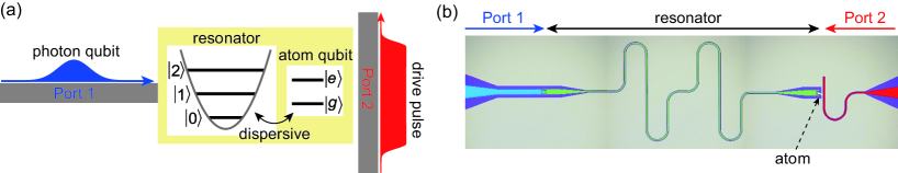
Figure 1: Setup for the SWAP gate between superconducting-atom and microwave-photon qubits. (a) Schematic of the setup. (b) False-colored optical micrograph of the actual device.

The setup for the present atom-photon SWAP gate is a common one in superconducting quantum computing: a superconducting atom is dispersively coupled to a microwave resonator, and transmission lines are attached to both of them (Fig. 1). One of the lines (Port 2) is coupled to the atom and a microwave drive pulse, which transforms the bare states of the atom-resonator system to the dressed ones within the pulse duration, is applied through this line. The other line (Port 1) is coupled to the resonator and a single microwave photon, which serves as a photon qubit, is input through this line synchronously with the drive pulse. The atom qubit is encoded on its ground and excited states, $|g\rangle$ and $|e\rangle$. The photon qubit is encoded on its two different carrier frequencies, $|\omega_{L}\rangle$ and $|\omega_{H}\rangle$, where $\omega_{L}$ ($\omega_{H}$) denotes the lower (higher) carrier frequency. The gate operation completes deterministically by bouncing the photon qubit applied through Port 1.

II.2 Principle of SWAP gate

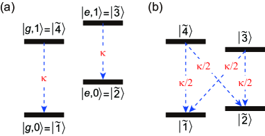
Figure 2: Level structure of the atom-resonator system. (a) Bare states, where the drive field from Port 2 is off. (b) Dressed states, where the drive field is on. Note that the energy diagram (b) is drawn in the frame rotating at the drive frequency $\omega_{\mathrm{d}}$.

Here, we outline the working principle of the present gate. We label the eigenstates of the atom-resonator system by $|a,n\rangle$, where $a=\{g,e\}$ and $n=\{0,1,\cdots\}$ respectively specify the atomic state and the photon number in the resonator. The atom-resonator system is in the dispersive coupling regime, and the eigenfrequencies are given by $\omega_{|g,n\rangle}=n\omega_{\mathrm{r}}$ and $\omega_{|e,n\rangle}=\omega_{\mathrm{ge}}+n(\omega_{\mathrm{r}}-2\chi)$, where $\omega_{\mathrm{ge}}$ and $\omega_{\mathrm{r}}$ are the renormalized frequencies of the atom and the resonator and $\chi$ is the dispersive shift. In the present atom-photon gate, we use the lowest four levels of the atom-resonator system ($a=\{g,e\}$ and $n=\{0,1\}$). The principal decay channel of this four-level system is the radiative decay of the resonator to Port 1 with a rate of $\kappa$. Therefore, when the drive field is off, the radiative decay within this four-level system occurs vertically with $\kappa$ [Fig. 2(a)].

During the interaction between the photon qubit and the atom-resonator system, we apply a microwave drive to the atom from Port 2. This drive field hybridizes the lower-two bare states $|g,0\rangle$ and $|e,0\rangle$ to form the dressed states $|\widetilde{1}\rangle$ and $|\widetilde{2}\rangle$. By switching on/off the drive field adiabatically, we can convert the bare and dressed states deterministically as $|g,0\rangle\leftrightarrow|\widetilde{1}\rangle$ and $|e,0\rangle\leftrightarrow|\widetilde{2}\rangle$. Similarly, the higher-two states are converted as $|e,1\rangle\leftrightarrow|\widetilde{3}\rangle$, and $|g,1\rangle\leftrightarrow|\widetilde{4}\rangle$. In addition to vertical decays ($|\widetilde{3}\rangle\to|\widetilde{2}\rangle$ and $|\widetilde{4}\rangle\to|\widetilde{1}\rangle$), oblique decays ($|\widetilde{3}\rangle\to|\widetilde{1}\rangle$ and $|\widetilde{4}\rangle\to|\widetilde{2}\rangle$) become allowed due to hybridization in a dressed-state basis.

In particular, under a proper choice of the frequency and power of the drive field, the four radiative decay rates take an identical value of $\kappa/2$ [Fig. 2(b)]. Then, the levels $|\widetilde{1}\rangle$, $|\widetilde{2}\rangle$ and $|\widetilde{j}\rangle$ ($j=3$ or 4) function as an “impedance-matched” $\Lambda$ system prop ; our_1 : if the system is in the state $|\widetilde{1}\rangle$ initially and a single photon with frequency $\omega_{j1}=\omega_{|\widetilde{j}\rangle}-\omega_{|\widetilde{1}\rangle}$ is input from Port 1, a Raman transition $|\widetilde{1}\rangle\to|\widetilde{j}\rangle\to|\widetilde{2}\rangle$ is deterministically induced. As a result, the $\Lambda$ system switches to the state $|\widetilde{2}\rangle$ and the input photon becomes down-converted to frequency $\omega_{j2}$ after reflection. In this study, we choose $j=4$ and set $\omega_{L}=\omega_{42}$ and $\omega_{H}=\omega_{41}$ as the lower and higher carrier frequencies of the photon qubit. The time evolution of the atom and photon qubits is then written as $|\widetilde{1},\omega_{H}\rangle\to|\widetilde{2},\omega_{L}\rangle$. The inverse process, $|\widetilde{2},\omega_{L}\rangle\to|\widetilde{1},\omega_{H}\rangle$, is also deterministic. In contrast, for the initial states of $|\widetilde{1},\omega_{L}\rangle$ and $|\widetilde{2},\omega_{H}\rangle$, the input photon is perfectly reflected as it is without interacting with the $\Lambda$ system, since the input photon is out of resonance of the $\Lambda$ system. Namely, $|\widetilde{1},\omega_{L}\rangle\to|\widetilde{1},\omega_{L}\rangle$ and $|\widetilde{2},\omega_{H}\rangle\to|\widetilde{2},\omega_{H}\rangle$. These four-time evolutions are summarized as

$$(\beta_{1}|\widetilde{1}\rangle+\beta_{2}|\widetilde{2}\rangle)\otimes(\gamma_{1}|\omega_{L}\rangle+\gamma_{2}|\omega_{H}\rangle)\to(\gamma_{1}|\widetilde{1}\rangle+\gamma_{2}|\widetilde{2}\rangle)\otimes(\beta_{1}|\omega_{L}\rangle+\beta_{2}|\omega_{H}\rangle),$$ (1)

where $\beta_{1},\cdots,\gamma_{2}$ are arbitrary coefficients satisfying $|\beta_{1}|^{2}+|\beta_{2}|^{2}=|\gamma_{1}|^{2}+|\gamma_{2}|^{2}=1$.

Before and after the interaction between the photon qubit and the atom-resonator system, we switch off the drive field. Therefore, the atom-resonator system returns to the bare state basis as $|\widetilde{1}\rangle=|g,0\rangle$ and $|\widetilde{2}\rangle=|e,0\rangle$. Omitting the resonator’s state, which is in the vacuum state at both the initial and final moments, Eq. (1) is rewritten as

$$(\beta_{1}|g\rangle+\beta_{2}|e\rangle)\otimes(\gamma_{1}|\omega_{L}\rangle+\gamma_{2}|\omega_{H}\rangle)\to(\gamma_{1}|g\rangle+\gamma_{2}|e\rangle)\otimes(\beta_{1}|\omega_{L}\rangle+\beta_{2}|\omega_{H}\rangle).$$ (2)

This is a SWAP gate between the atom qubit and the photon qubit applied through Port 1.

III demonstration of SWAP gate

In this section, we demonstrate the atom-photon SWAP gate. This should be done, in principle, by applying a single-photon pulse from Port 1 as the photon qubit. However, in this study, we use a weak coherent-state pulse instead, the mean photon number $|\alpha|^{2}$ of which is much smaller than unity. This pulse is dichromatic in general with the carrier frequencies $\omega_{L}$ and $\omega_{H}$ and has a Gaussian temporal profile with the pulse length of $t_{\mathrm{p}}=100$ ns. This is long enough to satisfy the condition for high-fidelity atom-photon gate, $t_{\mathrm{p}}\gg 1/\kappa$, where $\kappa$ is the resonator decay rate into Port 1 (see Table 3). If the initial states of the atom and photon qubits are $\beta_{1}|g\rangle+\beta_{2}|e\rangle$ and $\gamma_{1}|\omega_{L}\rangle+\gamma_{2}|\omega_{H}\rangle$, respectively, the initial state vector of the atom-photon system is written as

$$|\psi_{i}\rangle = (\beta_{1}|g\rangle+\beta_{2}|e\rangle)\otimes e^{-|\alpha|^{2}/2}\left[|0\rangle+\alpha(\gamma_{1}|\omega_{L}\rangle+\gamma_{2}|\omega_{H}\rangle)+\cdots\right],$$ (3)

where $\alpha$ represents the complex amplitude of the input photon-qubit pulse, and the dots represent the multiphoton components in the pulse, which are negligible when $|\alpha|^{2}\ll 1$. This state vector is rewritten as

$$|\psi_{i}\rangle = c_{1}|g,0\rangle+c_{2}|e,0\rangle+c_{3}|g,\omega_{L}\rangle+c_{4}|e,\omega_{L}\rangle+c_{5}|g,\omega_{H}\rangle+c_{6}|e,\omega_{H}\rangle+\cdots,$$ (4)

where $(c_{1},\cdots,c_{6})=e^{-|\alpha|^{2}/2}\times(\beta_{1},\beta_{2},\alpha\beta_{1}\gamma_{1},\alpha\beta_{2}\gamma_{1},\alpha\beta_{1}\gamma_{2},\alpha\beta_{2}\gamma_{2})$.

The atom-photon SWAP gate is completed by bouncing the photon qubit at the capacitance connecting Port 1 and the resonator. The time evolution is given by Eq. (1) and results in the following final state vector,

$$|\psi_{f}\rangle = c_{1}|g,0\rangle+c_{2}|e,0\rangle+c_{3}|g,\omega_{L}\rangle+c_{5}|e,\omega_{L}\rangle+c_{4}|g,\omega_{H}\rangle+c_{6}|e,\omega_{H}\rangle+\cdots.$$ (5)

III.1 State transfer: photon to atom

III.1.1 Procedures for density matrix estimation

In order to demonstrate the atom-photon SWAP gate, we confirm the bidirectional state transfer between the atom and photon qubits. Here, we demonstrate the photon-to-atom state transfer. We denote the density matrix of the final atom qubit by $\hat{\rho}^{(\mathrm{c})}_{\mathrm{a}}$, where the superscript (c) implies that the input photon-qubit pulse is in a coherent state. The matrix element of $\hat{\rho}^{(\mathrm{c})}_{\mathrm{a}}$ is given by $\hat{\rho}^{(\mathrm{c})}_{\mathrm{a},mn}=\mathrm{Tr}_{\mathrm{p}}\{\langle m|\psi_{f}\rangle\langle\psi_{f}|n\rangle\}$, where $m,n(=g,e)$ specify the atomic state and $\mathrm{Tr}_{\mathrm{p}}$ takes the trace over the photonic states. From Eq. (5), $\rho^{\mathrm{(c)}}_{\mathrm{a},ee}$ and $\rho^{\mathrm{(c)}}_{\mathrm{a},eg}$ are given, up to the second order in $|\alpha|$, by

$$\rho^{(\mathrm{c})}_{\mathrm{a},ee} \approx |\beta_{2}|^{2}+|\alpha|^{2}(|\gamma_{2}|^{2}-|\beta_{2}|^{2}),$$ (6)

$$\rho^{(\mathrm{c})}_{\mathrm{a},eg} \approx \beta_{1}^{*}\beta_{2}+|\alpha|^{2}(\gamma_{1}^{*}\gamma_{2}-\beta_{1}^{*}\beta_{2}).$$ (7)

On the other hand, our target quantity here is the density matrix $\hat{\rho}^{(\mathrm{s})}_{\mathrm{a}}$ of the final atom qubit assuming the single-photon input. If the SWAP gate is performed with the single-photon input, the final atomic state is $\gamma_{1}|g\rangle+\gamma_{2}|e\rangle$ [see Eq. (2)]. Therefore, $\rho^{(\mathrm{s})}_{\mathrm{a},ee}=|\gamma_{2}|^{2}$ and $\rho^{(\mathrm{s})}_{\mathrm{a},eg}=\gamma_{1}^{*}\gamma_{2}$.

Thus, we can reproduce the target density matrix $\hat{\rho}^{\mathrm{(s)}}_{\mathrm{a}}$ from the measurable one $\hat{\rho}^{(\mathrm{c})}_{\mathrm{a}}$ by the following procedures: Setting the initial atomic state at $|g\rangle$ [namely, $(\beta_{1},\beta_{2})=(1,0)$], we perform the atom-photon SWAP gate and measure the final atomic density matrix elements $\rho^{(\mathrm{c})}_{\mathrm{a},ee}$ and $\rho^{(\mathrm{c})}_{\mathrm{a},eg}$. Putting $(\beta_{1},\beta_{2})=(1,0)$ in Eqs. (6) and (7), they are expected to behave as $\rho^{(\mathrm{c})}_{\mathrm{a},ee}=|\alpha|^{2}|\gamma_{2}|^{2}$ and $\rho^{(\mathrm{c})}_{\mathrm{a},eg}=|\alpha|^{2}\gamma_{1}^{*}\gamma_{2}$. Therefore, by varying the mean photon number $|\alpha|^{2}$ and measuring the slopes of these quantities, two of the target density matrix elements are estimated as

$$\rho^{(\mathrm{s})}_{\mathrm{a},ee} = \frac{d}{d|\alpha|^{2}}\rho^{(\mathrm{c})}_{\mathrm{a},ee},$$ (8)

$$\rho^{(\mathrm{s})}_{\mathrm{a},eg} = \frac{d}{d|\alpha|^{2}}\rho^{(\mathrm{c})}_{\mathrm{a},eg}.$$ (9)

The other elements are determined by $\rho^{(\mathrm{s})}_{\mathrm{a},ge}=(\rho^{(\mathrm{s})}_{\mathrm{a},eg})^{*}$ and $\rho^{(\mathrm{s})}_{\mathrm{a},gg}=1-\rho^{(\mathrm{s})}_{\mathrm{a},ee}$.

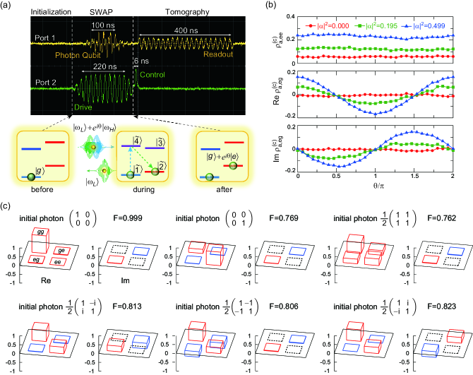
Figure 3: Photon-to-atom state transfer. (a) Pulse sequence depicted in the intermediate frequencies (IFs) and the energy diagrams before, during, and after the SWAP gate. In the energy diagrams, the initial atom (photon) qubit is assumed to be in the polar (equator) state, namely, $(\beta_{1},\beta_{2})=(1,0)$ and $(\gamma_{1},\gamma_{2})=(1,e^{i\theta})/\sqrt{2}$. (b) Measured density matrix elements ($\rho^{(\mathrm{c})}_{\mathrm{a},ee}$, $\mathrm{Re}\rho^{(\mathrm{c})}_{\mathrm{a},eg}$, $\mathrm{Im}\rho^{(\mathrm{c})}_{\mathrm{a},eg}$) of the final atom qubit for the coherent-state input. The initial atom (photon) qubit is in the ground (equator) state, and the phase $\theta$ of the photon qubit is varied continuously. The mean photon number $|\alpha|^{2}$ in the photon-qubit pulse is indicated. (c) Estimated density matrix $\hat{\rho}_{\mathrm{a}}^{(\mathrm{s})}$ of the final atom qubit assuming the single-photon input. Positive, negative, and zero matrix elements are drawn in red, blue, and black dotted lines, respectively. The fidelity to the initial photon qubit is indicated.

III.1.2 Pulse sequence

The pulse sequence to measure the density matrix $\hat{\rho}^{(\mathrm{c})}_{\mathrm{a}}$ of the final atom qubit is shown in Fig. 3(a). The measurement is composed of three steps. (i) Initialization: we wait for complete de-excitation of the atom applying no pulses. (ii) SWAP gate: from Port 2, we apply a drive pulse with a flat-top envelope at $\omega_{\rm d}/2\pi=5.785$ GHz to the atom to implement an impedance-matched $\Lambda$ system [Fig. 2(b)]. Within the drive pulse duration, we input from Port 1 the photon-qubit pulse with a Gaussian envelope, which is dichromatic ($\omega_{L}/2\pi=\omega_{42}/2\pi=10.208$ GHz and $\omega_{H}/2\pi=\omega_{41}/2\pi=10.266$ GHz) in general. Note that the photon-qubit pulse in Fig. 3(a) does not have a clear Gaussian envelope because of its dichromatic nature. (iii) Tomography: we first apply a short control pulse (no pulse, $\pi$ pulse, or 4 kinds of $\pi/2$ pulse) with a Gaussian envelope at $\omega_{\rm ge}/2\pi=5.839$ GHz to the atom and then dispersively read out the atomic state with a rectangular pulse at $\omega_{\rm r}/2\pi=10.258$ GHz.

III.1.3 Results and discussion

The measured density matrix elements $\rho^{(\mathrm{c})}_{\mathrm{a},ee}$ and $\rho^{(\mathrm{c})}_{\mathrm{a},eg}$ of the final atom qubit are shown in Fig. 3(b), where the initial atom (photon) qubit is in the ground (equator) state, namely, $(\beta_{1},\beta_{2})=(1,0)$ and $(\gamma_{1},\gamma_{2})=(1,e^{i\theta})/\sqrt{2}$. We observe that $\rho^{(\mathrm{c})}_{\mathrm{a},ee}$ is independent of the phase $\theta$ of the initial photon qubit and increases in proportion to $|\alpha|^{2}$, and that $\rho^{(\mathrm{c})}_{\mathrm{a},eg}$ is an oscillating function of $\theta$ and its amplitude grows by increasing $|\alpha|^{2}$. These observations are in qualitative accordance with Eqs. (6) and (7), which predicts that $\rho^{(\mathrm{c})}_{\mathrm{a},ee}=|\alpha|^{2}/2$ and $\rho^{(\mathrm{c})}_{\mathrm{a},eg}=|\alpha|^{2}e^{i\theta}/2$. These results indicate that the phase information of the initial photon qubit is successfully transferred to the final atom qubit.

In Fig. 3(c), we present the density matrix $\hat{\rho}^{(\mathrm{s})}_{\mathrm{a}}$ of the final atom qubit assuming the single-photon input, estimated by the aforementioned procedures. More details on the estimation are presented in Appendix A. The initial photon qubit is in one of the six cardinal states [$|\omega_{L}\rangle$, $|\omega_{H}\rangle$, and $(|\omega_{L}\rangle+e^{in\pi/4}|\omega_{H}\rangle)/\sqrt{2}$ for $n=0,\cdots,3$]. The agreement between the initial photon and final atom qubits is fairly good and the averaged fidelity for the six cardinal states reaches 0.829. The principal origin of the infidelity would be the short $T_{1}$ ($\sim 0.9~{}\mu$s) of the superconducting atom, which is comparable to the time required for the state tomography of the final atom qubit. An exceptionally high fidelity is attained when the initial photon qubit is in $|\omega_{L}\rangle$ [first panel in Fig. 3(c)]. This is because the atom remains in the ground state ($|g,0\rangle\approx|\widetilde{1}\rangle$) throughout the gate operation and is unaffected by the short $T_{1}$.

III.2 State transfer: atom to photon

III.2.1 Procedures for density matrix estimation

Here, we demonstrate the atom-to-photon state transfer. More concretely, from the amplitudes of the final photon-qubit pulse (after reflection in Port 1) for the coherent-state input, we estimate the density matrix $\hat{\rho}_{\mathrm{p}}^{(\mathrm{s})}$ of the final photon qubit assuming the single-photon input. The final amplitude $\xi(t)$ is given by $\xi(t)=\langle\psi_{f}|\hat{a}|\psi_{f}\rangle$, where $\hat{a}$ is the annihilation operator for a propagating photon in Port 1. Using Eq. (5), $\xi(t)$ is given, up to the first order in $|\alpha|$, by

$$\xi(t) = \alpha(|\beta_{1}|^{2}\gamma_{1}+\beta_{1}\beta_{2}^{*}\gamma_{2})\psi_{L}(t)+\alpha(\beta_{1}^{*}\beta_{2}\gamma_{1}+|\beta_{2}|^{2}\gamma_{2})\psi_{H}(t),$$ (10)

where $\psi_{L(H)}(t)=\langle 0|\hat{a}|\omega_{L(H)}\rangle$ is the single-photon amplitude of the lower (higher) frequency component. When the initial photon-qubit pulse is monochromatic at $\omega_{L}$, the final amplitude $\xi_{L}(t)$ is given, by putting $(\gamma_{1},\gamma_{2})=(1,0)$ in Eq. (10), by

$$\xi_{L}(t) = \alpha|\beta_{1}|^{2}\psi_{L}(t)+\alpha\beta_{1}^{*}\beta_{2}\psi_{H}(t).$$ (11)

This equation implies that the initial monochromatic pulse may become dichromatic after reflection, depending on the initial atomic state. However, when the atom is in the ground state initially, the final pulse remains monochromatic at $\omega_{L}$. We denote its amplitude by $\zeta_{L}(t)$. Putting $(\beta_{1},\beta_{2})=(1,0)$ in Eq. (11), we have

$$\zeta_{L}(t) = \alpha\psi_{L}(t).$$ (12)

Similarly, when the initial pulse is monochromatic at $\omega_{H}$, the final amplitude $\xi_{H}(t)$ is given by

$$\xi_{H}(t) = \alpha\beta_{1}\beta_{2}^{*}\psi_{L}(t)+\alpha|\beta_{2}|^{2}\psi_{H}(t).$$ (13)

$\zeta_{H}(t)$ is the result for the initial atom being in the excited state. Putting $(\beta_{1},\beta_{2})=(0,1)$ in Eq. (13), we have

$$\zeta_{H}(t) = \alpha\psi_{H}(t).$$ (14)

We denote the overlap integral between $\zeta_{i}(t)$ and $\xi_{j}(t)$ ($i,j=L,H$) by

$$\eta_{ij}=\int dt\zeta_{i}^{*}(t)\xi_{j}(t).$$ (15)

Since $\psi_{L}(t)$ and $\psi_{H}(t)$ are orthogonal to each other due to the different carrier frequencies, we obtain $\eta_{LL}=C|\alpha|^{2}|\beta_{1}|^{2}$, $\eta_{HH}=C|\alpha|^{2}|\beta_{2}|^{2}$, $\eta_{LH}=C|\alpha|^{2}\beta_{1}\beta_{2}^{*}$, and $\eta_{HL}=C|\alpha|^{2}\beta_{1}^{*}\beta_{2}$, where $C=\int dt|\psi_{j}(t)|^{2}$ ($j=L,H$).

On the other hand, our target quantity here is the density matrix $\hat{\rho}_{\mathrm{p}}^{(\mathrm{s})}$ of the final photon qubit assuming the single-photon input. From the right-hand side of Eq. (2), we immediately have $\hat{\rho}_{\mathrm{p}}^{(\mathrm{s})}=(\beta_{1}|\omega_{L}\rangle+\beta_{2}|\omega_{H}\rangle)(\beta_{1}^{*}\langle\omega_{L}|+\beta_{2}^{*}\langle\omega_{H}|)$. Therefore, the following 2$\times$2 matrix,

$$\hat{\eta} = \frac{1}{\eta_{LL}+\eta_{HH}}\left(\begin{array}[]{cc}\eta_{LL}&\eta_{LH}\\ \eta_{HL}&\eta_{HH}\end{array}\right),$$ (18)

is identical to the target density matrix $\hat{\rho}_{\mathrm{p}}^{(\mathrm{s})}$ in principle.

Thus, we can construct the target density matrix $\hat{\rho}^{\mathrm{(s)}}_{\mathrm{p}}$ from the measured amplitudes of the final photon-qubit pulse by the following procedures: Preliminarily, setting the initial atom-qubit state at $|g\rangle$ ($|e\rangle$), we apply a monochromatic photon-qubit pulse at $\omega_{L}$ ($\omega_{H}$) and measure the final amplitude $\zeta_{L}(t)$ [$\zeta_{H}(t)$]. Then, for an arbitrary initial atom-qubit state, we apply a monochromatic pulse at $\omega_{L}$ ($\omega_{H}$) and measure the final amplitude $\xi_{L}(t)$ [$\xi_{H}(t)$]. We construct a 2$\times$2 matrix $\hat{\eta}$ from the overlap integrals between these output amplitudes [Eqs. (15) and (18)]. $\hat{\eta}$ is identical to the target density matrix $\hat{\rho}_{\mathrm{p}}^{(\mathrm{s})}$ in principle, but is non-Hermitian in practice (see Table 2). We estimate a proper one by the protocol presented in Appendix B.

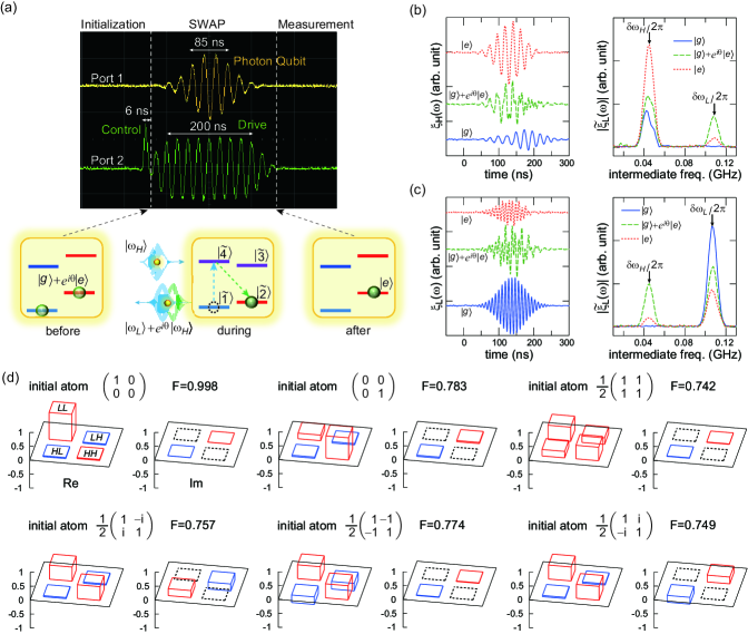
Figure 4: Atom-to-photon state transfer. (a) Pulse sequence depicted in the intermediate frequencies (IFs) and the energy diagrams before, during, and after the SWAP gate. In the energy diagrams, the initial atom (photon) qubit is assumed to be in the equator (polar) state, namely, $(\beta_{1},\beta_{2})=(1,e^{i\theta})/\sqrt{2}$ and $(\gamma_{1},\gamma_{2})=(0,1)$ D (b) Measured amplitude of the output photon-qubit pulse for its initial frequency set at $\omega_{H}$: time domain (left) and frequency domain (right). The initial atom-qubit state (ground, equator, or excited) is indicated. Since the four equator states yield similar spectra, only one of them is plotted. The mean photon number in the input pulse is $|\alpha|^{2}=0.101$. The time-domain amplitudes are measured by an analog-to-digital converter and are averaged over $1.5\times 10^{4}$ times. (c) The same plots as (b) for the initial frequency of the photon-qubit pulse set at $\omega_{L}$. (d) Estimated density matrix $\hat{\rho}^{(\mathrm{s})}_{\mathrm{p}}$ of the final photon qubit assuming the single-photon input. Positive (negative) values are indicated by red (blue) bars. The fidelity to the initial atom qubit is indicated.

III.2.2 Pulse sequence

The pulse sequence to measure the amplitude $\xi(t)$ of the final photon-qubit pulse is shown in Fig. 4(a). The measurement is composed of three steps. (i) Initialization: we wait for complete deexcitation of the atom. We then apply a control pulse with a Gaussian envelope at $\omega_{\rm ge}/2\pi=5.835$ GHz from Port 2 to the atom to prepare it in one of the six cardinal states. (ii) SWAP gate: from Port 2, we apply a drive pulse with a flat-top envelope at $\omega_{\rm d}/2\pi=5.775$ GHz to the atom to constitute an impedance-matched $\Lambda$ system [Fig. 1(b)]. Within the pulse duration, we input from Port 1 a weak monochromatic (at $\omega_{L}/2\pi=10.201$ GHz or $\omega_{H}/2\pi=10.263$ GHz) photon-qubit pulse with a Gaussian envelope. (iii) Measurement: we measure the amplitude of the reflected photon-qubit pulse in Port 1, which is dichromatic in general. Note that $\omega_{L}$ and $\omega_{H}$ are slightly different from those in the “photon-to-atom” experiment, since the experiment was performed in the different cooling down of our dilution refrigerator (see Table 3 for details on the experimental parameters).

All microwave pulses in Fig. 4(a) are generated by single-sideband modulation and are shown in the intermediate frequencies (IFs), similarly to those in Fig. 3(a). A carrier microwave at $\omega_{\rm c}/2\pi=10.308$ GHz and a Gaussian envelope with IF $=\delta\omega_{H}/2\pi=0.045$ GHz ($\delta\omega_{L}/2\pi=0.107$ GHz) are mixed by an IQ mixer, obtaining the photon pulse with $\omega_{H}=\omega_{\rm c}-\delta\omega_{H}$ ($\omega_{L}=\omega_{\rm c}-\delta\omega_{L}$). The final photon-qubit pulses after reflection by the atom are measured by an analog-digital converter after downconverted at $\omega_{\rm c}$ in order to extract the signals at $\delta\omega_{H}$ ($\delta\omega_{L}$) as shown in the left panels in Figs. 4(b) and (c). The frequency-domain plots [right panels in Figs. 4(b) and (c)] are obtained by applying the fast Fourier transform (FFT) to the time-domain plots.

III.2.3 Results and discussions

In Fig. 4(b), we plot the final amplitudes of the photon-qubit pulse in the time [$\xi_{H}(t)$, Eq. (13)] and frequency [$\widetilde{\xi}_{H}(\omega)$, Fourier transform of $\xi_{H}(t)$] domains, fixing its initial frequency at $\omega_{H}$ and varying the initial atomic state. Predictions by Eq. (13) are as follows. (i) Putting $(\beta_{1},\beta_{2})=(0,1)$, we have $\xi_{H}(t)=\alpha\psi_{H}(t)$. Namely, when the atom is in the excited state initially, the final amplitude is monochromatic at $\omega_{H}$, unchanged from the initial one. (ii) Putting $(\beta_{1},\beta_{2})=(1,e^{i\theta})/\sqrt{2}$, we have $\xi_{H}(t)=(\alpha/2)[e^{-i\theta}\psi_{L}(t)+\psi_{H}(t)]$. Namely, when the atom is in the equator state initially, the final amplitude is dichromatic at $\omega_{L}$ and $\omega_{H}$ with equal magnitudes. (iii) Putting $(\beta_{1},\beta_{2})=(1,0)$, we have $\xi_{H}(t)=0$. Namely, when the atom is in the ground state initially, the final amplitude vanishes. We observe that the measured amplitudes in Fig. 4(b) are in qualitative agreement with these predictions. However, we also find discrepancies from these predictions, such as non-vanishing signal at $\omega_{H}$ for the initial atom in $|g\rangle$ and appearance of the $\omega_{L}$ component for the initial atom in $|e\rangle$. We attribute the principal reason for the former discrepancy to the imperfect constitution of an impedance-matched $\Lambda$ system [namely, difference in the $|\widetilde{4}\rangle\to|\widetilde{1}\rangle$ and $|\widetilde{4}\rangle\to|\widetilde{2}\rangle$ decay rates in Fig. 2(b)] and the latter to the imperfect initialization of the atom qubit, both of which originate in the fluctuation in the transition frequency $\omega_{\mathrm{ge}}$ of the superconducting atom. Note that the drastic attenuation of the final amplitude in (iii) does not mean the decrease of the reflected photon in Port 1: the input photon is mostly downconverted to $\omega_{L}$ but its amplitude is unobservable in this experiment due to the inelasticity of scattering. This quantum process (single-photon Raman interaction dop_th_1 ; dop_th_2 ; dop_th_3 ; our_1 ; our_2 ; dayan1 ; dayan2 ; dayan3 ) has been applied for the single microwave photon detection spd1 ; spd2 . Figure 4(c) shows the results for the initial frequency of the photon-qubit pulse tuned at $\omega_{L}$. The results are contrastive to those in Fig. 4(b) and are in qualitative accordance with Eq. (11).

In Fig. 4(d), we present the density matrix $\hat{\rho}^{(\mathrm{s})}_{\mathrm{p}}$ of the final photon qubit assuming the single-photon input, estimated by the aforementioned procedures. More details on estimation are presented in Appendix B. The fidelity to the initial atom qubit, which is prepared to be in one of the six cardinal states, is fairly good and the averaged fidelities reaches 0.801. An exceptionally high fidelity is attained when the initial atom is in $|g\rangle$ [first panel in Fig. 4(c)], because the atom remains in the ground state throughout the gate operation and is unaffected by the short $T_{1}(\sim 0.9~{}\mu$s) of the superconducting atom. We observe that, when the initial atom qubit is in the equator states, the fidelities become substantially lower than those for the photon-to-atom state transfer [Fig. 3(c)]. Presently, we do not fully understand the reason for that. One possible reason might be that the amplitude of the frequency-converted component [$\omega_{L/H}$ component in the right panel of Fig. 4(b/c)], which becomes observable only when the initial atom is in a superposition state, is more fragile against the pure dephasing than the amplitude of the unconverted component.

IV conclusion

We have demonstrated a deterministic SWAP gate between a superconducting qubit and a frequency-encoded microwave-photon qubit. More concretely, we have confirmed the bidirectional (photon-to-atom and atom-to-photon) transfer of the qubit state. The photon qubit for this gate is a single-photon pulse propagating in a waveguide, but we used a weak coherent-state pulse instead for demonstration.

To confirm the photon-to-atom qubit transfer, we applied a monochromatic or dichromatic photon-qubit pulse, which corresponds to one of the six cardinal states of the photon qubit, to the dressed atom-resonator coupled system (impedance-matched $\Lambda$ system). After reflection of this pulse, we performed a state tomography of the final atom qubit. From the dependencies of the density matrix elements on the mean input photon number, we constructed the density matrix of the final atom qubit assuming the single-photon input. The fidelity to the initial photon qubit reaches 0.829 on average. On the other hand, to confirm the atom-to-photon qubit transfer, we prepared the initial atom qubit to be in one of the six cardinal states and applied a monochromatic photon-qubit pulse to the $\Lambda$ system. From the measured amplitudes of the final photon-qubit pulse, we constructed the density matrix of the final photon qubit assuming the single-photon input. The fidelity to the initial atom qubit reaches 0.801 on average.

Although the fidelities of the qubit-state transfer here are still insufficient for practical application, the principal reason for these infidelities is the short lifetime of the superconducting atom, which can readily be overcome with the current qubit fabrication technology. We hope that the present scheme for the atom-photon SWAP gate, equipped with distinct merits such as simplicity of the setup and in-situ gate tunability, would help the distributed quantum computation with superconducting qubits in near future.

Appendix A Density matrix estimation: photon to atom

Here, we present the details on the density matrix estimation for the photon-to-atom state transfer [Fig. 3(c)].

A.1 State tomography of $\hat{\rho}^{(\mathrm{c})}_{\mathrm{a}}$

We first discuss how to determine the density matrix $\hat{\rho}^{(\mathrm{c})}_{\mathrm{a}}$ of the final atom qubit from the measurement data. In the tomography stage of Fig. 3(a), we first perform one of the six kinds of one-qubit gates to the atom. The unitary matrices corresponding to these gates are

$$\hat{U}_{j} = \begin{cases}\hat{I}&(j=1)\\ \hat{\sigma}_{x}&(j=2)\\ (\hat{I}-i\cos(\frac{j\pi}{2})\hat{\sigma}_{x}-i\sin(\frac{j\pi}{2})\hat{\sigma}_{y})/\sqrt{2}&(j=3,\cdots,6)\end{cases}.$$ (19)

We measure the excitation probability of the atom by dispersive readout. We denote the measured probability after $j$th gate by $\widetilde{p}_{j}$. We estimate the atomic density matrix $\hat{\rho}^{(\mathrm{c})}_{\mathrm{a}}$ from the measurement data set $(\widetilde{p}_{1},\cdots,\widetilde{p}_{6})$.

We parameterize $\hat{\rho}^{(\mathrm{c})}_{\mathrm{a}}$ as

$$\hat{\rho}^{(\mathrm{c})}_{\mathrm{a}} = (\hat{I}+a_{x}\hat{\sigma}_{x}+a_{y}\hat{\sigma}_{y}+a_{z}\hat{\sigma}_{z})/2,$$ (20)

where $a_{x}$, $a_{y}$, and $a_{z}$ are the Bloch vector components, which are real and satisfy $a_{x}^{2}+a_{y}^{2}+a_{z}^{2}\leq 1$. With this density matrix, the expected excitation probability $p_{j}$ after $j$th gate is given by $p_{j}=\mathrm{Tr}\{(\hat{1}+\hat{\sigma}_{z})\hat{U}_{j}\hat{\rho}^{(\mathrm{c})}_{\mathrm{a}}\hat{U}_{j}^{\dagger}\}/2$. Using Eqs. (19) and (20), we have $p_{1}=(1+a_{z})/2$, $p_{2}=(1-a_{z})/2$, $p_{3}=(1+a_{x})/2$, $p_{4}=(1+a_{y})/2$, $p_{5}=(1-a_{x})/2$, and $p_{6}=(1-a_{y})/2$. We determine the parameters $a_{x}$, $a_{y}$, and $a_{z}$ so as to minimize the sum of squared errors,

$$S(a_{x},a_{y},a_{z}) = \sum_{j=1}^{6}(p_{j}-\widetilde{p}_{j})^{2}.$$ (21)

This is rewritten as $S(a_{x},a_{y},a_{z})=(a_{x}-\overline{a}_{x})^{2}+(a_{y}-\overline{a}_{y})^{2}+(a_{z}-\overline{a}_{z})^{2}+\cdots$, where

$$\overline{a}_{x} = \widetilde{p}_{3}-\widetilde{p}_{5},$$ (22)

$$\overline{a}_{y} = \widetilde{p}_{4}-\widetilde{p}_{6},$$ (23)

$$\overline{a}_{z} = \widetilde{p}_{1}-\widetilde{p}_{2}.$$ (24)

Therefore, if the point P$(\overline{a}_{x},\overline{a}_{y},\overline{a}_{z})$ is inside of the unit sphere, $S$ is minimized at this point. In contrast, if the point P is out of the unit sphere, $S$ is minimized at the projection of point P to the unit-sphere surface in the radial direction. Therefore,

$$(a_{x},a_{y},a_{z}) = \frac{(\overline{a}_{x},\overline{a}_{y},\overline{a}_{z})}{\max\left(1,\sqrt{\overline{a}_{x}^{2}+\overline{a}_{y}^{2}+\overline{a}_{z}^{2}}\right)}.$$ (25)

In Table 1, setting the initial photon qubit at $|\psi_{\mathrm{p}}\rangle=(|\omega_{L}\rangle-i|\omega_{H}\rangle)/\sqrt{2}$ for example, we present the measurement data set $(\widetilde{p}_{1},\cdots,\widetilde{p}_{6})$ and the estimated Bloch vector components for various input photon number $|\alpha|^{2}$.

Table 1: Measured excitation probabilities $\widetilde{p}_{j}$ and the estimated Bloch vector components $(a_{x},a_{y},a_{z})$ for various input photon number $|\alpha|^{2}$. The initial photon-qubit state is $|\psi_{\mathrm{p}}\rangle=(|\omega_{L}\rangle-i|\omega_{H}\rangle)/\sqrt{2}$.

$|\alpha|^{2}$	$\widetilde{p}_{1}$	$\widetilde{p}_{2}$	$\widetilde{p}_{3}$	$\widetilde{p}_{4}$	$\widetilde{p}_{5}$	$\widetilde{p}_{6}$	$a_{x}$	$a_{y}$	$a_{z}$
$0.0000$	$0.0371$	$0.9226$	$0.4953$	$0.4965$	$0.4812$	$0.4821$	$0.0141$	$0.0144$	$-0.8855$
$0.1950$	$0.0721$	$0.8306$	$0.4795$	$0.5452$	$0.4823$	$0.4124$	$-0.0028$	$0.1328$	$-0.7585$
$0.4992$	$0.1950$	$0.7358$	$0.4800$	$0.6442$	$0.4697$	$0.3084$	$0.0103$	$0.3358$	$-0.5408$

A.2 Estimation of $\hat{\rho}^{(\mathrm{s})}_{\mathrm{a}}$ from $\hat{\rho}^{(\mathrm{c})}_{\mathrm{a}}$

Here, we discuss how to estimate the atomic density matrix $\hat{\rho}^{(\mathrm{s})}_{\mathrm{a}}$ assuming the single-photon input from the one $\hat{\rho}^{(\mathrm{c})}_{\mathrm{a}}$ for the coherent-state input. Similarly to Eq. (20), we parametrize the target density matrix as

$$\hat{\rho}^{(\mathrm{s})}_{\mathrm{a}} = (\hat{I}+b_{x}\hat{\sigma}_{x}+b_{y}\hat{\sigma}_{y}+b_{z}\hat{\sigma}_{z})/2.$$ (26)

Then, From Eqs. (8) and (9), we obtain

$$b_{x} = \frac{da_{x}}{d|\alpha|^{2}},$$ (27)

$$b_{y} = \frac{da_{y}}{d|\alpha|^{2}},$$ (28)

$$b_{z} = \frac{da_{z}}{d|\alpha|^{2}}-1.$$ (29)

Therefore, we can estimate $b_{x}$ from the dependence of $a_{x}$ on the mean input photon number $|\alpha|^{2}$. Assuming a linear dependence and employing the least square method, we determine the slope $\overline{b}_{x}$ from the data set of $\{|\alpha|^{2(j)},a_{x}^{(j)}\}$ for $j=1,\cdots,N$, where $N$ is the number of the data set. $\overline{b}_{x}$ is then given by

$$\overline{b}_{x} = \frac{NC_{2}-C_{3}C_{4}}{NC_{1}-C_{3}^{2}},$$ (30)

where $C_{1}=\sum_{j}(|\alpha|^{2(j)})^{2}$, $C_{2}=\sum_{j}|\alpha|^{2(j)}a_{x}^{(j)}$, $C_{3}=\sum_{j}|\alpha|^{2(j)}$, and $C_{4}=\sum_{j}a_{x}^{(j)}$. $\overline{b}_{y}$ and $\overline{b}_{z}$ are determined similarly. If the point Q$(\overline{b}_{x},\overline{b}_{y},\overline{b}_{z})$ is outside of the unit sphere, we project this point to the unit-sphere surface in the radial direction. Therefore,

$$(b_{x},b_{y},b_{z}) = \frac{(\overline{b}_{x},\overline{b}_{y},\overline{b}_{z})}{\max\left(1,\sqrt{\overline{b}_{x}^{2}+\overline{b}_{y}^{2}+\overline{b}_{z}^{2}}\right)}.$$ (31)

From the data set presented in Table 1, we have $b_{x}=-0.0032$, $b_{y}=0.6459$, and $b_{z}=-0.3074$. Accordingly, $\rho^{(\mathrm{s})}_{\mathrm{a},ee}=(1+b_{z})/2=0.3463$ and $\rho^{(\mathrm{s})}_{\mathrm{a},eg}=(b_{x}+ib_{y})/2=-0.0016-0.3229i$ [the last panel in Fig. 3(c)].

Appendix B Density matrix estimation: atom to photon

Here, we present the details on the density matrix estimation for the atom-to-photon state transfer [Fig. 4(d)].

B.1 Estimation of $\hat{\rho}^{(\mathrm{s})}_{\mathrm{p}}$ from $\hat{\eta}$

According to the arguments in Sec. III.2, the matrix $\hat{\eta}$ constructed directly from the experimental data [Eqs. (15) and (18)] is, in principle, identical to the target density matrix $\hat{\rho}^{(\mathrm{s})}_{\mathrm{p}}$. However, as we observe in Table 2, $\hat{\eta}$ is non-Hermite in practice. We therefore estimate a proper density matrix $\hat{\rho}^{(\mathrm{s})}_{\mathrm{p}}$ from $\hat{\eta}$ by the following procedures.

Similarly to Eq. (20), we parameterize the proper density matrix as

$$\hat{\rho}^{(\mathrm{s})}_{\mathrm{p}} = (\hat{I}+c_{x}\hat{\sigma}_{x}+c_{y}\hat{\sigma}_{y}+c_{z}\hat{\sigma}_{z})/2,$$ (32)

where $c_{x}$, $c_{y}$, and $c_{z}$ are real and satisfy $c_{x}^{2}+c_{y}^{2}+c_{z}^{2}\leq 1$. We choose $c_{x}$, $c_{y}$ and $c_{z}$ so as to minimize the distance $L$ between $\hat{\eta}$ and $\hat{\rho}^{(\mathrm{s})}_{\mathrm{p}}$, which we quantify by

$$L(c_{x},c_{y},c_{z}) = \sum_{j=x,y,z}|\langle\hat{\sigma}_{j}\rangle_{\eta}-\langle\hat{\sigma}_{j}\rangle_{\rho}|^{2},$$ (33)

where $\langle\hat{\sigma}_{j}\rangle_{\eta}=\mathrm{Tr}\{\hat{\sigma}_{j}\hat{\eta}\}$ and $\langle\hat{\sigma}_{j}\rangle_{\rho}=\mathrm{Tr}\{\hat{\sigma}_{j}\hat{\rho}^{(\mathrm{s})}_{\mathrm{p}}\}$. Since $\langle\hat{\sigma}_{x}\rangle_{\eta}=\eta_{LH}+\eta_{HL}$, $\langle\hat{\sigma}_{y}\rangle_{\eta}=i(\eta_{LH}-\eta_{HL})$, $\langle\hat{\sigma}_{z}\rangle_{\eta}=\eta_{LL}-\eta_{HH}$, $\langle\hat{\sigma}_{x}\rangle_{\rho}=c_{x}$, $\langle\hat{\sigma}_{y}\rangle_{\rho}=c_{y}$, and $\langle\hat{\sigma}_{z}\rangle_{\rho}=c_{z}$, Eq. (33) is rewritten as $L(x,y,z)=(c_{x}-\overline{c}_{x})^{2}+(c_{y}-\overline{c}_{y})^{2}+(c_{z}-\overline{c}_{z})^{2}+\cdots$, where

$$\overline{c}_{x} = \mathrm{Re}(\eta_{LH}+\eta_{HL}),$$ (34)

$$\overline{c}_{y} = \mathrm{Im}(\eta_{HL}-\eta_{LH}),$$ (35)

$$\overline{c}_{z} = \mathrm{Re}(\eta_{LL}-\eta_{HH}).$$ (36)

Therefore, if the point R$(\overline{c}_{x},\overline{c}_{y},\overline{c}_{z})$ is inside of the unit sphere, $L$ is minimized at this point. On the other hand, if the point R is out of the unit sphere, $L$ is minimized at the projection of point R to the unit sphere. Therefore,

$$(c_{x},c_{y},c_{z}) = \frac{(\overline{c}_{x},\overline{c}_{y},\overline{c}_{z})}{\max\left(1,\sqrt{\overline{c}_{x}^{2}+\overline{c}_{y}^{2}+\overline{c}_{z}^{2}}\right)}.$$ (37)

In Table 2, we present the matrix elements of $\hat{\eta}$ and $\hat{\rho}^{(\mathrm{s})}_{\mathrm{p}}$ for various input photon number $|\alpha|^{2}$. The initial atom-qubit state is chosen as $|\psi_{\mathrm{a}}\rangle=(|g\rangle-i|e\rangle)/\sqrt{2}$ for example, and the fidelity is that between the initial atom and final photon qubits, $F=\langle\psi_{\mathrm{a}}|\hat{\rho}^{(\mathrm{s})}_{\mathrm{p}}|\psi_{\mathrm{a}}\rangle$. We observe that the estimated density matrix is mostly insensitive to the input photon number $|\alpha|^{2}$. In Fig. 4(c), we employ the averaged density matrix over the four cases as $\hat{\rho}^{(\mathrm{s})}_{\mathrm{p}}$.

Table 2: Elements of density matrices $\hat{\eta}$ and $\hat{\rho}^{(\mathrm{s})}_{\mathrm{p}}$. The initial atom-qubit state is $|\psi_{\mathrm{a}}\rangle=(|g\rangle-i|e\rangle)/\sqrt{2}$ for example and the mean input photon number $|\alpha|^{2}$ is varied. $\rho^{(\mathrm{s})}_{\mathrm{p},HH}(=1-\rho^{(\mathrm{s})}_{\mathrm{p},LL})$ and $\rho^{(\mathrm{s})}_{\mathrm{p},HL}(=\rho^{(\mathrm{s})*}_{\mathrm{p},LH})$ are not shown.

$|\alpha|^{2}$	$\eta_{LL}$	$\eta_{LH}$	$\eta_{HL}$	$\eta_{HH}$	$\rho^{(\mathrm{s})}_{\mathrm{p},HH}$	$\rho^{(\mathrm{s})}_{\mathrm{p},HL}$	fidelity
$0.048$	$0.515+0.057i$	$-0.095+0.187i$	$-0.003-0.277i$	$0.485-0.057i$	$0.485$	$-0.049-0.232i$	$0.732$
$0.101$	$0.509+0.043i$	$-0.113+0.215i$	$0.042-0.333i$	$0.491-0.043i$	$0.491$	$-0.036-0.274i$	$0.774$
$0.163$	$0.502+0.056i$	$-0.106+0.204i$	$0.030-0.282i$	$0.498-0.056i$	$0.498$	$-0.038-0.243i$	$0.743$
$0.206$	$0.503+0.058i$	$-0.121+0.162i$	$0.038-0.330i$	$0.497-0.058i$	$0.497$	$-0.042-0.246i$	$0.746$
average					$0.493$	$-0.041-0.249i$	$0.749$

Appendix C Experimental information

C.1 Experimental setup

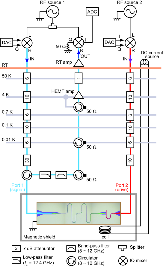
Figure 5: Schematic of the experimental setup.

Figure 5 shows a schematic of the measurement setup composed of room-temperature microwave instruments and low-temperature wirings with microwave components in a cryogen-free ³He/⁴He dilution refrigerator.

The photon-qubit (drive) pulses applied to Port $1$ ($2$) are generated by mixing the continuous microwave from the RF source $1$ ($2$) with pulses that have an intermediate frequency (IF) generated by a DAC (digital to analog converter) with a sampling rate of $1$ GHz. The Gaussian pulses are used for the photon-qubit pulses, while the flat-top pulses, in which the rising and falling edges of the pulse envelope are smoothed by a Gaussian function with full width at half maximum of $40$ ns in its voltage amplitude, are employed for the drive pulses.

The signal pulses are heavily attenuated by a series of attenuators implemented in the input microwave semi-rigid cable with a total attenuation of $68$ dB and applied to the $\lambda/2$ resonator through a circulator to separate the input and reflected signal. The reflected signal is led to a cryogenic HEMT amplifier mounted at a $4$ K stage of the dilution refrigerator via low-pass and band-pass filters and three circulators with 50 $\Omega$ terminations and amplified by $\sim 38$ dB followed by further amplification with a room-temperature low-noise amplifier, whose gain is $\sim 33$ dB. The output signal is down-converted to IF at an IQ mixer using a continuous microwave split the same signal used for the photon-qubit pulse generation. The I component of the reflected signals is sampled at $1.6$ GHz/s by an ADC (analog to digital converter).

The drive pulses are applied through the input microwave semi-rigid cable with a total attenuation of $48$ dB to control the states of an atom.

C.2 Device and parameters

A device employed in our experiments is composed of a $\lambda/2$ superconducting coplanar waveguide resonator and a superconducting flux qubit containing three Josephson junctions [Fig. 1(b)]. They are coupled capacitively and operated in the dispersive regime. We adopted the same design and fabrication processes for the device described in Ref. spd2 ; our_2 .

In Table 3, we summarize the system parameters for the SWAP experiments described in the main text. Since each SWAP experiment was performed in the different cooling down of our dilution refrigerator, $\omega_{\rm ge}$ and related parameters ($\chi$, $\omega_{\mathrm{d}}$, $\omega_{L}$ and $\omega_{H}$) changed slightly. The other parameters ($\omega_{r}$ and $\kappa$) are independent of $\omega_{\rm ge}$ and remain unchanged.

Table 3: Device parameters for the “photon to atom” and the “atom to photon” SWAP experiments (unit: GHz).

Parameters	Photon $\rightarrow$ Atom	Atom $\rightarrow$ Photon
$\omega_{\rm r}/2\pi$	10.258	10.258
$\omega_{\rm ge}/2\pi$	5.839	5.835
$2\chi/2\pi$	0.073	0.073
$\kappa/2\pi$	0.024	0.024
$\omega_{\rm d}/2\pi$	5.785	5.775
$\omega_{L}/2\pi$	10.208	10.201
$\omega_{H}/2\pi$	10.266	10.263

References

- (1) F. Arute et al., Quantum supremacy using a programmable superconducting processor, Nature 574, 505 (2019).
- (2) Y. Wu et al., Strong Quantum Computational Advantage Using a Superconducting Quantum Processor, Phys. Rev. Lett. 127, 180501 (2021).
- (3) J. I. Cirac, A. K. Ekert, S. F. Huelga, and C. Macchiavello, Distributed quantum computation over noisy channels, Phys. Rev. A 59, 4249 (1999).
- (4) Y. L. Lim, A. Beige, and L. C. Kwek, Repeat-Until-Success Linear Optics Distributed Quantum Computing, Phys. Rev. Lett. 95, 030505 (2005).
- (5) D. Cuomo, M. Caleffi, and A. S. Cacciapuoti, Towards a distributed quantum computing ecosystem, IET Quantum Commun., 1, 3 (2020).
- (6) S. Bravyi, O. Dial, J. M. Gambetta, D. Gil, and Z. Nazario, The Future of Quantum Computing with Superconducting Qubits, J. Appl. Phys. 132, 160902 (2022).
- (7) A. Reiserer and G. Rempe, Cavity-based quantum networks with single atoms and optical photons, Rev. Mod. Phys. 87, 1379 (2015).
- (8) N. Meher and S. Sivakumar, Quantum information processing in cavities: A review, arXiv:2204.01322.
- (9) J. T. Shen and S. Fan, Coherent photon transport from spontaneous emission in one-dimensional waveguides, Opt. Lett. 30, 2001 (2005).
- (10) O. Astafiev, A. M. Zagoskin, A. A. Abdumalikov Jr, Y. A. Pashkin, T. Yamamoto, K. Inomata, Y. Nakamura, and J. S. Tsai, Resonance fluorescence of a single artificial atom, Science 327, 840 (2010).
- (11) I. C. Hoi, C. M. Wilson, G. Johansson, J. Lindkvist, B. Peropadre, T. Palomaki, and P. Delsing, Microwave quantum optics with an artificial atom in one-dimensional open space, New J. Phys. 15, 025011 (2013).
- (12) A. F. van Loo, A. Fedorov, K. Lalumiere, B. C. Sanders, A. Blais, and A. Wallraff, Photon-mediated interactions between distant artificial atoms, Science 342, 1494 (2013).
- (13) X. Gu, A. F. Kockum, A. Miranowicz, Y. X. Liu, and F. Nori, Microwave photonics with superconducting quantum circuits, Phys. Rep. 718-719, 1 (2017).
- (14) S. Kono, K. Koshino, D. Lachance-Quirion, A. F. van Loo, Y. Tabuchi, A. Noguchi, and Y. Nakamura, Breaking the trade-off between fast control and long lifetime of a superconducting qubit, Nat. Commun. 11, 3683 (2020).
- (15) A. Blais, A. L. Grimsmo, S. M. Girvin, A. Wallraff, Circuit Quantum Electrodynamics, Rev. Mod. Phys. 93, 25005 (2021)
- (16) K. Koshino, K. Inomata, Z. Lin, Y. Nakamura and T. Yamamoto, Theory of microwave single-photon detection using an impedance-matched system, Phys. Rev. A 91, 043805 (2015).
- (17) K. Inomata, Z. R. Lin, K. Koshino, W. D. Oliver, J. S. Tsai, T. Yamamoto, and Y. Nakamura, Single microwave-photon detector using an artificial -type three-level system, Nat. Commun. 7, 12303 (2016).
- (18) J. Govenius, R. E. Lake, K. Y. Tan, and M. Mottonen, Detection of Zeptojoule Microwave Pulses Using Electrothermal Feedback in Proximity-Induced Josephson Junctions, Phys. Rev. Lett. 117, 030802 (2016).
- (19) S. Kono, K. Koshino, Y. Tabuchi, A. Noguchi, and Y. Nakamura, Quantum non-demolition detection of an itinerant microwave photon, Nat. Phys. 14, 546 (2018).
- (20) J.-C. Besse, S. Gasparinetti, M. C. Collodo, T. Walter, P. Kurpiers, M. Pechal, C. Eichler, and A. Wallraff, Single-Shot Quantum Nondemolition Detection of Individual Itinerant Microwave Photons, Phys. Rev. X 8, 021003 (2018).
- (21) R. Lescanne, S. Deleglise, E. Albertinale, U. Reglade, T. Capelle, E. Ivanov, T. Jacqmin, Z. Leghtas, and E. Flurin, Irreversible Qubit-Photon Coupling for the Detection of Itinerant Microwave Photons, Phys. Rev. X 10, 021038 (2020).
- (22) J. I. Cirac, P. Zoller, H. J. Kimble, and H. Mabuchi, Quantum State Transfer and Entanglement Distribution among Distant Nodes in a Quantum Network, Phys. Rev. Lett. 78, 3221 (1997).
- (23) Y. Yin, Y. Chen, D. Sank, P. J. J. O’Malley, T. C. White, R. Barends, J. Kelly, E. Lucero, M. Mariantoni, A. Megrant, C. Neill, A. Vainsencher, J. Wenner, A. N. Korotkov, A. N. Cleland, and J. M. Martinis, Catch and Release of Microwave Photon States, Phys. Rev. Lett. 110, 107001 (2013).
- (24) M. Pechal, L. Huthmacher, C. Eichler, S. Zeytinoglu, A. A. Abdumalikov, Jr., S. Berger, A. Wallraff, and S. Filipp, Microwave-Controlled Generation of Shaped Single Photons in Circuit Quantum Electrodynamics, Phys. Rev. X 4, 041010 (2014).
- (25) P. Kurpiers, P. Magnard, T. Walter, B. Royer, M. Pechal, J. Heinsoo, Y. Salathe, A. Akin, S. Storz, J.-C. Besse, S. Gasparinetti, A. Blais and A. Wallraff, Deterministic quantum state transfer and remote entanglement using microwave photons, Nature 558, 264 (2018).
- (26) P. Campagne-Ibarcq, E. Zalys-Geller, A. Narla, S. Shankar, P. Reinhold, L. Burkhart, C. Axline, W. Pfaff, L. Frunzio, R. J. Schoelkopf, and M. H. Devoret, Deterministic Remote Entanglement of Superconducting Circuits through Microwave Two-Photon Transitions, Phys. Rev. Lett. 120, 200501 (2018).
- (27) N. Leung, Y. Lu, S. Chakram, R. K. Naik, N. Earnest, R. Ma, K. Jacobs, A. N. Cleland, and D. I. Schuster, Deterministic bidirectional communication and remote entanglement generation between superconducting qubits, npj Quantum inf. 5, 18 (2019).
- (28) K. Reuer, J. C. Besse, L. Wernli, P. Magnard, P. Kurpiers, G. J. Norris, A. Wallraff, and C. Eichler, Realization of a Universal Quantum Gate Set for Itinerant Microwave Photons, Phys. Rev. X 12, 011008 (2022).
- (29) K. Koshino, K. Inomata, Z. R. Lin, Y. Tokunaga, T. Yamamoto, and Y. Nakamura, Theory of Deterministic Entanglement Generation between Remote Superconducting Atoms, Phys. Rev. Applied 7, 064006 (2017).
- (30) D. Pinotsi and A. Imamoglu, Single Photon Absorption by a Single Quantum Emitter, Phys. Rev. Lett. 100, 093603 (2008).
- (31) K. Koshino, S. Ishizaka and Y. Nakamura, Deterministic photon-photon gate using a system, Phys. Rev. A 82, 010301(R) (2010).
- (32) D. Witthaut and A. S. Sorensen, Photon scattering by a three-level emitter in a one-dimensional waveguide, New J. Phys. 12, 043052 (2010).
- (33) K. Koshino, K. Inomata, T. Yamamoto and Y. Nakamura, Implementation of an Impedance-Matched System by Dressed-State Engineering, Phys. Rev. Lett. 111, 153601 (2013).
- (34) K. Inomata, K. Koshino, Z. R. Lin, W. D. Oliver, J. S. Tsai, Y. Nakamura and T. Yamamoto, Microwave Down-Conversion with an Impedance-Matched System in Driven Circuit QED, Phys. Rev. Lett. 113, 063064 (2014).
- (35) I. Shomroni, S. Rosenblum, Y. Lovsky, O. Bechler, G. Guendelman, B. Dayan, All-optical routing of single photons by a one-atom switch controlled by a single photon, Science 345, 903 (2014).
- (36) S. Rosenblum, O. Bechler, I. Shomroni, Y. Lovsky, G. Guendelman, and B. Dayan, Extraction of a single photon from an optical pulse, Nature Photonics 10, 19 (2016).
- (37) O. Bechler, A. Borne, S. Rosenblum, G. Guendelman, O. E. Mor, M. Netser, T. Ohana, Z. Aqua, N. Drucker, R. Finkelstein, Y. Lovsky, R. Bruch, D. Gurovich, E. Shafir, and B. Dayan, A passive photon-atom qubit swap operation, Nat. Phys. 14, 996 (2018).
- (38) A. Blais, R.-S. Huang, A. Wallraff, S. M. Girvin, and R. J. Schoelkopf, Cavity quantum electrodynamics for superconducting electrical circuits: An architecture for quantum computation, Phys. Rev. A 69, 062320 (2004).
- (39) P. Krantz, M. Kjaergaard, F. Yan, T. P. Orlando, S. Gustavsson, and W. D. Oliver A Quantum Engineer’s Guide to Superconducting Qubits, Appl. Phys. Rev. 6, 021318 (2019)
- (40) G. Burkard, D. Loss, and D. P. DiVincenzo, Coupled quantum dots as quantum gates, Phys. Rev. B 59, 2070 (1999).
- (41) H. Fan, V. Roychowdhury, and T. Szkopek, Optimal two-qubit quantum circuits using exchange interactions, Phys. Rev. A 72, 052323 (2005).
- (42) Y. Zhou and G.-F. Zhang, gate in the presence of spin-orbit coupling in coupled quantum dots, Opt. Commun. 316, 22 (2014)
- (43) W. Q. Liu and H. R. Wei, Implementations of more general solid-state (SWAP)1/m and controlled-(swap)1/m gates, New J. Phys. 21, 103018 (2019).
- (44) S. Clemmen, A. Farsi, S. Ramelow, and A. L. Gaeta, Ramsey Interference with Single Photons, Phys. Rev. Lett. 117, 223601 (2016).
- (45) J. M. Lukens and P. Lougovski, Frequency-encoded photonic qubits for scalable quantum information processing, Optica 4, 8 (2017).
- (46) S. C. Connell, J. Scarabel, E. M. Bridge, K. Shimizu, V. Blums, M. Ghadimi, M. Lobino, and E. W. Streed, Ion-photonic frequency qubit correlations for quantum networks, J. Phys. B: At. Mol. Opt. Phys. 54, 175503 (2021)
- (47) M. L. Chan, Z. Aqua, A. Tiranov, B. Dayan, P. Lodahl, and A. S. Sorensen, Quantum state transfer between a frequency-encoded photonic qubit and a quantum-dot spin in a nanophotonic waveguide, Phys. Rev. A 105, 062445 (2022).
- (48) J. Ilves, S. Kono, Y. Sunada, S. Yamazaki, M. Kim, K. Koshino, and Y. Nakamura, On-demand generation and characterization of a microwave time-bin qubit, npj Quantum Inf. 6, 34 (2020).