On Fairness and Stability: Is Estimator Variance a Friend or a Foe?

Abstract.

The error of an estimator can be decomposed into a (statistical) bias term, a variance term, and an irreducible noise term. When we do bias analysis, formally we are asking the question: “how good are the predictions?” The role of bias in the error decomposition is clear: if we trust the labels/targets, then we would want the estimator to have as low bias as possible, in order to minimize error. Fair machine learning is concerned with the question: “Are the predictions equally good for different demographic/social groups?” This has naturally led to a variety of fairness metrics that compare some measure of statistical bias on subsets corresponding to socially privileged and socially disadvantaged groups. In this paper we propose a new family of performance measures based on group-wise parity in variance. We demonstrate when group-wise statistical bias analysis gives an incomplete picture, and what group-wise variance analysis can tell us in settings that differ in the magnitude of statistical bias. We develop and release an open-source library that reconciles uncertainty quantification techniques with fairness analysis, and use it to conduct an extensive empirical analysis of our variance-based fairness measures on standard benchmarks.

1. Introduction

The error of an estimator can be decomposed into a (statistical) bias term, a variance term, and an irreducible noise term. When we do bias analysis, formally we are asking the question: “how good are the predictions?” The role of bias in the error decomposition is clear: if we trust the labels/targets, then we would want the estimator to have as low bias as possible, in order to minimize error. Fair machine learning (fair-ML) is concerned with the question: “Are the predictions equally good for different demographic or socioeconomic groups?” One way to define equally good is to require that the statistical bias of the estimator on samples from different demographic groups should be comparable. In other words, unbiasedness is a fairness desideratum if we trust the data labels. This has naturally led to a variety of proposed fairness metrics, usually defined as the difference or the ratio of a measure of statistical bias (such as the True Positive Rate or the True Negative Rate) computed on different test subsets — corresponding to socially privileged and socially disadvantaged groups, respectively.

A complementary statistical question concerns the variance of the estimator. When we do variance analysis, formally we are asking the question: “How stable are the predictions?” The role of variance in the error decomposition is subtle: it is unclear whether low variance is always a desirable property. For example, in a biased estimator — whose predictions deviate from the true value — high variance can have a corrective effect on some samples. From a philosophical perspective, randomness is morally neutral, and so the effects of large variance can be morally more acceptable (and fairness-enhancing) than the effects of a systematic skew. Randomization is, of course, already used in algorithmic fairness research (Dwork et al., 2012), and it is an essential building block of the differential privacy framework (Dwork, 2011).

In this paper, our goal is to understand the role of estimator variance from a fairness perspective — what behavior of estimator variance is morally desirable? The dominant belief in fair-ML is that both stability and fairness are simultaneously desirable, that is, that we want to construct estimators that have parity in statistical bias across groups (are “fair”) and have low variance (are “stable”) (Huang and Vishnoi, 2019; Friedler et al., 2019). Our insights provide a more nuanced picture of the stability desideratum in fair-ML and uncover a novel fairness-variance-accuracy trade-off.

Contributions:

1. We propose a new family of performance measures based on group-wise parity in variance in Section 2, and demonstrate their usefulness on folktables (Ding et al., 2021) and COMPAS (Angwin et al., 2016) benchmarks in Section 4.

2. We clarify the relationship between fairness and stability: If a model is fair (in the sense of exhibiting low disparity in statistical bias), then we also desire it to be stable (in the sense of exhibiting overall low variance). However, instability (high variance) does not imply unfairness (high disparity in statistical bias)! Indeed, as we show empirically in Section 4, there is a fairness-variance-accuracy trade-off, where:

   • Parity in variance and parity in statistical bias (“fairness”) can come at the cost of overall model accuracy, as we demonstrate empirically using the logistic regression model for the ACSEmployment task on the folktables benchmark (Ding et al., 2021).

   • Variance can have a corrective effect on both fairness and the overall accuracy for models that have reasonably high overall accuracy. For example, we observe the MLP classifier on the ACSEmployment task on folktables and Decision Tree on COMPAS (Angwin et al., 2016) trading-off model stability to gain parity in statistical bias.

   • Conversely, for a classifier that has low overall accuracy, attempting to improve overall stability (low variance) and parity in stability across groups (parity in variance) negates any potentially corrective effect of estimator variance, and thereby leads to model unfairness. We observe this empirically for the XGBoost classifier on COMPAS.

3. We developed and publicly release a software library called Virny that reconciles uncertainty quantification techniques with fairness analysis/auditing frameworks. Using this library, it is easy to measure stability (estimator variance) and fairness for several protected groups, and their intersections. We use this library in our own empirical analysis.

Roadmap.

In Section 2, we present metrics for model performance. We first review influential fairness metrics, expressing them as ratios or differences of measures of statistical bias (Section 2.1). Next, we introduce several measures of estimator variance from robustness and uncertainty quantification literature, and propose a new family of performance metrics, expressed as the difference or ratio of these variance metrics (Section 2.2). This reconciles statistical bias-based and variance-based analysis of parity in estimator performance on different subgroups, and provides a richer picture of algorithmic discrimination, as we empirically demonstrate in Section 4. In Section 3 we introduce a new software library — Virny—to compute statistical bias and variance metrics on subgroups of interest, and to compose parity-based performance metrics from them. In Section 4, we report our empirical findings on folktables and COMPAS benchmarks, introduce the fairness-variance-accuracy trichotomy, and give a critical comparison of our proposed variance metrics with existing metrics. We conclude and discuss avenues for exciting future work in Section 5.

2. Metrics for Model Performance

Literature on fair-ML abounds with measures of models “fairness”. Here, we first summarize some influential fairness measures that are stated as the ratio or the difference of measures of statistical bias computed on different demographic groups in Section 2.1, and go on to define a new family of variance-based measures in Section 2.2.

Notation.

Let $Y$ be the target or true outcome, $X$ be the covariates or features, and $A$ be the set of protected/sensitive attributes. To start, we limit our treatment to binary group membership, letting $A=1$ denote the privileged group and $A=0$ denote the disadvantaged group. We are interested to construct an estimator $\hat{Y}=f(X,A)$ that predicts $Y$, with the help of a suitable loss function. In fair-ML, we apply additional constraints on the interaction between $\hat{Y}$, $Y$ and $A$ in order to ensure that the estimator $\hat{Y}$ does not discriminate on the basis of sensitive attributes $A$. Different notions of fairness are formalized as different constraints, and a violation of the fairness constraint is usually defined as the corresponding measure of model unfairness, as we will discuss next.

2.1. Measures of Model (Un)Fairness

2.1.1. Equalized Odds

The fairness criterion of Equalized Odds from Hardt et al. (2016) is defined as:

$$P(\hat{Y}=1|A=0,Y=y)=P(\hat{Y}=1|A=1,Y=y),y\in\{0,1\}$$

For $Y=1$ (the positive outcome), this fairness constraint requires parity in true positive rates (TPR) across the groups $A=0$ and $A=1$, and for $Y=0$ (the negative outcome), the constraint requires parity in false positive rates (FPR). A violation of this constraint (i.e., the disparity in TPR and FPR across groups) is reported as a measure of model unfairness. In our paper, we refer to TPR and FPR as the base measures, and we say that the fairness criterion of Equalized Odds is composed as the difference between these base measures computed for the disadvantaged group ($A=0$, which we call dis) and for the privileged group ($A=1$, which we call priv), respectively.

$$\text{Equalized Odds Violation (True Positive)}=\Delta\text{TPR}=P(\hat{Y}=1|A=0,Y=1)-P(\hat{Y}=1|A=1,Y=1)$$

$$\text{Equalized Odds Violation (False Positive)}=\Delta\text{FPR}=P(\hat{Y}=1|A=0,Y=0)-P(\hat{Y}=1|A=1,Y=0)$$

We will now rewrite other influential fairness measures (Chouldechova, 2017; Kleinberg et al., 2017) as the difference or ratio between different the base measures on the dis and priv groups.

2.1.2. Disparate Impact

Inspired by the 4/5th’s rule in legal doctrines, Disparate Impact has been formulated as a fairness measure:

$$\text{Disparate Impact}=\mathcal{Q}(\text{Positive Rate})=\frac{P(\hat{Y}=1|A=0)}{P(\hat{Y}=1|A=1)}$$

$P(\hat{Y}=1)$ is simply the Positive Rate of the estimator, and so the measure of Disparate Impact is composed as the ratio of the Positive Rate on the dis and priv groups, respectively.

2.1.3. Statistical Parity Difference

Similarly, Statistical Parity is the fairness criterion that asks that comparable proportions of samples from each protected group receive the positive outcome:

$$P(\hat{Y}=1|A=0)=P(\hat{Y}=1|A=1)$$

Statistical parity difference (SPD) is a popular fairness metric composed simply as the difference between the estimator’s Positive Rate on dis and priv groups, respectively.

$$\text{Statistical Parity Difference}=\Delta(\text{Positive Rate})=P(\hat{Y}=1|A=0)-P(\hat{Y}=1|A=1)$$

2.1.4. Accuracy Parity

Accuracy parity is also commonly reported, and is computed as the difference in accuracy on dis and priv samples.

$$\text{Accuracy Parity}=\Delta(\text{Accuracy})=\frac{P(\hat{Y}=1|A=0,Y=1)+P(\hat{Y}=0|A=0,Y=0)}{P(\hat{Y}=1|A=0,Y=1)+P(\hat{Y}=1|A=0,Y=0)+P(\hat{Y}=0|A=0,Y=1)+P(\hat{Y}=0|A=0,Y=0)}$$

$$-\frac{P(\hat{Y}=1|A=1,Y=1)+P(\hat{Y}=0|A=1,Y=0)}{P(\hat{Y}=1|A=1,Y=1)+P(\hat{Y}=1|A=1,Y=0)+P(\hat{Y}=0|A=1,Y=1)+P(\hat{Y}=0|A=1,Y=0)}$$

2.2. Measures of Model (In)Stability

We now introduce several variance-based metrics. We will introduce several base measures of model variance first, as this requires some reconciliation with uncertainty quantification and robustness literature, and then define the corresponding variance-based measures of model instability on different groups.

To measure the variation in model output, we will use the popular bootstrap technique (Efron and Tibshirani, 1994). This involves constructing multiple training sets by sampling with replacement from the given training set, and then fitting estimators (with the same architecture and hyper-parameters) on these bootstrapped training sets. This allows us to construct a predictive distribution from the outputs of each trained model, instead of a single point estimate of the predicted probability. We can thereby compute different measures of variation between the predictions of the ensemble of estimators for the same data point, and use it to approximate the variance of a single model trained on the full dataset. We provide more details of our implementation of these techniques in Sections 3 and 4.

2.2.1. Label Stability

Label Stability (Darling and Stracuzzi, 2018) is defined as the normalized absolute difference between the number of times a sample is classified as positive or negative:

$$\text{Label Stability}=\frac{|\sum_{i=1}^{b}\mathbbm{1}[p_{\theta_{i}}(x)==1]-\sum_{i=1}^{b}\mathbbm{1}[p_{\theta_{i}}(x)==0]|}{b}$$

where $x$ is an unseen test sample, and $p_{\theta_{i}}(x)$ is the prediction of the $i^{\text{th}}$ model in the ensemble that has $b$ estimators.

Recall that we are using the bootstrap to construct an ensemble of predictors to approximate the variance of a single estimator fit on the entire dataset. Label stability is a measure of disagreement between estimators in the ensemble: If the absolute difference is large, the label is more stable. If the difference is exactly zero, then the estimator is said to be “highly unstable” because a test sample is equally likely to be classified as positive or negative by the ensemble.

We define the Label Stability Ratio as a new parity measure. It is computed as the ratio of the average Label Stability on samples from the disadvantaged (dis) group and the privileged (priv) group respectively.

2.2.2. Jitter

Jitter (Liu et al., 2022a) is a measure of the disparities of the model’s predictions for each individual test example. It reuses a notion of Churn (Milani Fard et al., 2016) to define a ”pairwise jitter”:

$$J_{i,j}\left(p_{\theta}\right)=\operatorname{Churn}_{i,j}\left(p_{\theta}\right)=\frac{\left|p_{\theta i}(x)\neq p_{\theta j}(x)\right|_{x\in X}}{|X|}$$

where $x$ is an unseen test sample, and $p_{\theta i}(x)$, $p_{\theta j}(x)$ are the predictions of the $i^{\text{th}}$ and $j^{\text{th}}$ estimator in the ensemble for $x$, respectively.

To compute the variability over all models in the ensemble, we need to average pairwise jitters over all pairs of models. This more general definition is called Jitter:

$$J\left(p_{\theta}\right)=\frac{\sum_{\forall i,j\in N}J_{i,j}\left(p_{\theta}\right)}{N\cdot(N-1)\cdot\frac{1}{2}}\text{, where }i<j$$

We define Jitter Parity as the difference of the average Jitter on samples from the dis and priv groups, respectively.

2.2.3. Standard Deviation and Inter-Quantile Range

The bootstrap can also be used to compute the standard deviation (Std) and the inter-quantile range (IQR) of the predicted probabilities of the ensemble, as an approximation of the spread in predictions of a single model trained on the full dataset.

We compute the standard deviation (Std) and IQR on different groups (dis and priv), and compose the group-wise difference as Std Parity and IQR Parity, respectively.

We will empirically demonstrate the usefulness of these variance-based metrics, especially where statistical-bias based measures fail to provide a complete picture of model performance, in Section 4. We will use a software library we developed to support this empirical analysis, and describe it next.

3. The Virny software library

In order to reconcile the reporting of statistical bias-based and variance-based performance measures discussed in Section 2, we developed Virny — a Python library for auditing model stability and fairness. The Virny library was developed based on three fundamental principles: 1) easy extensibility of model analysis capabilities; 2) compatibility to user-defined/custom datasets and model types; 3) simple composition of parity metrics based on context of use.

Virny decouples model auditing into several stages, including: subgroup metrics computation, group metrics composition, and metrics visualization and reporting. This gives data scientists and practitioners more control and flexibility to use the library for both model development and monitoring post-deployment.

3.1. Comparison with existing fairness libraries

Many toolkits dedicated to measuring bias and fairness have been released in the past couple of years. The majority of these toolkits are easily extensible, can measure a list of fairness metrics, and create detailed reports and visualizations. For example, AI Fairness 360 (Bellamy et al., 2018) is an extensible Python toolkit for fairness researchers and industry practitioners that can detect, explain, and mitigate unwanted algorithmic bias. Aequitas (Saleiro et al., 2018) is another fairness auditing toolbox for both data scientists and policymakers. It concentrates on detailed explanations of how it should be used in a public policy context, including a “Fairness Tree” that guides the user to select suitable fairness metrics for their decision-making context. FairLearn (Bird et al., 2020) provides an interactive visualization dashboard and implements unfairness mitigation algorithms. These components help with navigating trade-offs between fairness and model performance.

Similarly, LiFT (Vasudevan and Kenthapadi, 2020) can measure a set of fairness metrics, but additionally, it focuses on scalable metric computation for large ML systems. Authors have shown how bias measurement and mitigation tools can be integrated with production ML systems and, at the same time, how to enable monitoring and mitigation at each stage of the ML lifecycle. Finally, fairlib (Han et al., 2022) implements a broad range of bias mitigation approaches and supports the analysis of neural networks for complex computer vision and natural language processing tasks. In addition, the analysis module of fairlib provides an interactive model comparison to explore the effects of different mitigation approaches.

Virny distinguishes itself from the existing libraries in three key aspects. First, our software library instantiates our conceptual contribution, allowing the data scientist to understand the role of estimator variance in assessing model fairness. Virny supports the measurement of both statistical bias and variance metrics for a set of initialized models, both overall on the full test set and broken down by user-defined subgroups of interest.

Second, Virny provides several APIs for metrics computation, including an interface for the analysis of a set of initialized models based on multiple executions and random seeds. This interface enables a detailed model audit, and supports reliable and reproducible analysis of model performance.

Third, our library allows data scientists to specify multiple sensitive attributes, as well as their intersections, for analysis. For example, Virny can audit statistical bias and variance with respect to all of the following simultaneously: sex, race, age, sex&race, and race&age. We also support the definition of non-binary sensitive attributes (although we limit our experimental evaluation in Section 4 to binary groups). We hope that this flexibility in selecting datasets, models, metrics and subgroups of interest will help usher in an era of research where measuring and reporting a variety of metrics of model performance on different subgroups is the norm, and not a specialized research interest of the few.

3.2. Architecture

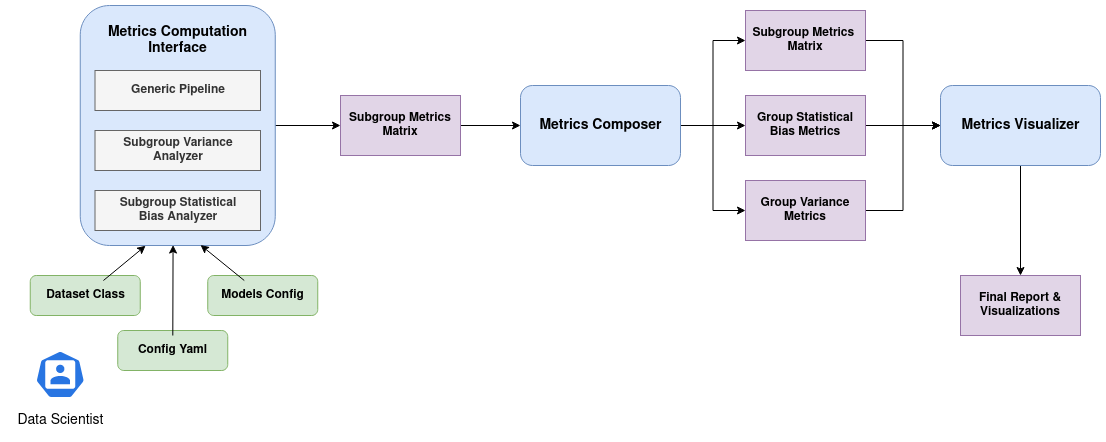
Figure 1. Virny Architecture

Figure 1 shows how Virny constructs a pipeline for model analysis. Pipeline stages are shown in blue, and the output of each stage is shown in purple. Each analysis pipeline has three processing stages: subgroup metrics computation, group metrics composition, and metrics visualization and reporting. We will now describe each of them.

3.2.1. Inputs

To use Virny, the user needs to provide three inputs, namely:

• A dataset class is a for the user’s dataset that includes its descriptive attributes such a target column, numerical columns, categorical columns, etc. This class must be inherited from the $BaseDataset$ class, which was created for user convenience. The idea behind having a common base class is to standardize raw dataset pre-processing and feature creation and to simplify the logic for downstream metric computation.

• A config Yaml is a file that specifies the configuration parameters for Virny’s user interfaces for metrics computation. We adopt this user-specified configuration approach to allow more flexibility to users. For instance, users can easily shift from one experiment to another, having just one config yaml per experiment, without having to make any further modifications before using Virny’s user interfaces.

  The config file contains information such as the number of bootstrap samples to create (this is the number of estimators in our ensemble for variance analysis), the fraction of samples in each bootstrap sample, a list of random seeds, etc. Importantly, we ask the user to specify subgroups of interest in the dataset by simply passing a dictionary where key-value pairs specify the relevant column names and the values of the sensitive attribute of the groups of interest. Users can also specify intersectional groups here.

• Finally, a models config is a Python dictionary, where keys are model names and values are initialized models for analysis. This dictionary helps conduct audits of multiple models for one or multiple runs and analyze different types of models.

3.2.2. Subgroup metric computation

After the variables are input to a user interface, Virny creates a generic pipeline based on the input dataset class to hide pre-processing complexity (such as one-hot encoding categorical columns, scaling numerical columns, etc) and provide methods for subsequent model analysis. Later, this generic pipeline is used in subgroup analyzers to compute different sets of metrics. Our library implements a Subgroup Variance Analyzer and a Subgroup Statistical Bias Analyzer, and it is easily extensible to include other analyzers. We provide abstract analyzer classes for users to inherit from and to create custom analyzers. Once these analyzers finish computing metrics, their outputs are combined and returned as a pandas dataframe.

The Subgroup Variance Analyzer is responsible for computing our variance metrics (from Section 2.2) on the overall test set, as well as on subgroups of interest specified by the user. We use a simple bootstrapping approach (Efron and Tibshirani, 1994) to quantify estimator variance, as is common in uncertainty quantification literature (Darling and Stracuzzi, 2018; Liu et al., 2022b; Lum et al., 2022). However, instead of simply computing the standard deviation of the predictive distribution, we also compute additional metrics such as label stability, jitter and IQR (defined in Section 2.2). Similarly, the Subgroup Statistical Bias Analyzer computes statistical bias metrics (such as accuracy, TPR, FPR, TNR, and FNR) on the overall test set as well as for subgroups of interest.

3.2.3. Group metric composition

The Metrics Composer is responsible for the second stage of the model audit. Currently, it computes the statistical bias-based and variance-based parity metrics described in Section 2, but a user can compose additional metrics if desired. For example, the fairness measure of Disparate Impact is composed as the ratio of the Positive Rate computed on the priv and dis subgroups.

3.2.4. Metric visualization and reporting

The Metrics Visualizer unifies different processing steps on the composed metrics and creates various data formats to ease visualization. Users can use methods of this class to create custom plots for analysis. Additionally, these plots can be collected in an HTML report with comments for reporting.

3.3. User Interfaces

For the first library release, we have developed the following three user interfaces:

3.3.1. Single run, single model

This interface gives the ability to audit one model for one execution. Users can set a model seed or generate and record a random seed, and control the number of estimators for bootstrap, the fraction of samples used in each bootstrap sample, and the test set fraction. This interface returns a pandas dataframe of statistical bias and variance metrics for an input base model and stores results separately in a file.

3.3.2. Single run, multiple models

This interface extends the functionality of the previous interface to audit multiple models. It can be more convenient and speed up the computation of multiple metrics for all models.

3.3.3. Multiple runs, multiple models

This interface can be used for a more extensive model audit. Users specify a set of models to use and the seeds for each run. This interface then computes metrics for all specified models and seeds, and saves the results after each run. In addition to metrics, this interface stores the seeds used for each run, which can help maintain consistent and reproducible results, such as those reported in Section 4.

4. Experiments

We used the Virny library, presented in Section 3, to conduct an extensive empirical comparison of the behavior of the metrics described in Section 2, and evaluate the trade-offs between fairness, variance and accuracy.

4.1. Benchmarks

We used two fair-ml benchmarks for our evaluation, namely folktables and COMPAS.

Folktables (Ding et al., 2021) is constructed from census data from 50 US states for the years 2014-2018. We report results on the ACSEmployment task: a binary classification task of predicting whether an individual is employed. We report our results on data from Georgia from 2018. The dataset has 16 covariates, including age, schooling, and disability status, and contains about 200k samples, which we sub-sample down to 20k samples for computational feasibility.

COMPAS (Angwin et al., 2016) is perhaps the most influential dataset in fair-ML, released for public use by ProPublica as part of their seminal report titled “Machine Bias.” We use the binary classification task to predict violent recidivism. Covariates include sex, age, and information on prior criminal justice involvement. We use the version of COMPAS supported by FairLearn. FairLearn loads the dataset pre-split into training and test. We merge these into a single dataset and then perform different random splits. We use the full dataset with 5,278 samples.

Table 1. Demographic composition of folktables and COMPAS.

	sex$\_$race$\_$priv	sex$\_$race$\_$dis	sex$\_$priv	sex$\_$dis	race$\_$priv	race$\_$dis
folktables	0.322	0.177	0.484	0.516	0.661	0.339
COMPAS	0.083	0.491	0.188	0.812	0.404	0.596

We define binary groups with respect to two features, sex and race. Males are the privileged group in folktables, while females are the privileged group in COMPAS. Whites are the privileged group in both folktables and COMPAS. We also look at intersectional groups constructed from sex and race: (male, white) and (female, black) are the intersectionally privileged and disadvantaged groups in folktables respectively, while (female,white) and (male,black) are the intersectionally privileged and disadvantaged groups in COMPAS respectively. The proportion of demographic groups in folktables and COMPAS is reported in Table 1.

4.2. Model Training

In our experiments, we evaluate the performance of 6 different models, namely, Decision Tree (DT), Logistic Regression (LR), Random Forest (RF), XG-Boosted Trees (XGB), K-Neighbors classifier (kNN), and a Neural Network (historically called the Multi-layer Perceptron, or MLP). In each run, we randomly split the dataset into train-test-validation sets (80:10:10). We use the validation set to tune hyper-parameters once for each model type, for each dataset. We fit a single model on the complete train set and compute standard performance metrics (such as accuracy, TPR, FPR, TNR and FNR) both on the overall test set, and broken down by demographic groups listed in table 1. Next, we use the bootstrap to construct 200 different versions of the training set (each with a size of $80\%$ of the full training set) and use this to train an ensemble of 200 predictors. We compute the variance metrics described in Section 2.2 on the outputs of this ensemble. We repeat this procedure for 10 different seeds on COMPAS and for 6 different seeds on folktables.

4.3. Experimental Results

For our analysis we will focus on four dimensions of model performance:

1. Overall statistical bias: an accurate model has low statistical bias on the full test set.

2. Overall variance: a stable model has low variance on the full test set.

3. Disparity in statistical bias: a fair model shows parity in statistical bias on dis and priv groups.

4. Disparity in variance: a uniformly stable model shows parity in variance on dis and priv groups.

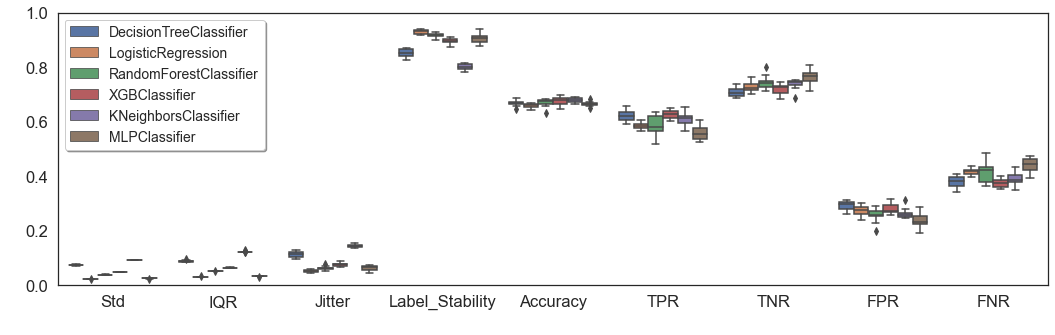
Figure 3. Statistical bias and variance metrics on COMPAS

The overall statistical bias and variance of different models is presented in Figure 2 for folktables and Figure 3 for COMPAS. Standard deviation (Std), inter-quantile range (IQR), jitter, and label stability are measures of estimator variance, while accuracy, TPR, FPR, TNR, and FNR are measures of statistical bias. We report all parity-based measures in Table 3 for folktables and Table 4 for COMPAS.

Cells are colored according to the following scheme: cells with values close to parity (0 for difference measures, 1 for ratio measures) are in green. Cells that report discrimination (i.e., disparity in favor of the priv group) are in pink, while those that report reverse discrimination (i.e., disparity in favor of the dis group) are in yellow. The positive class in folktables (positive employment status) is desirable, whereas in COMPAS (positive risk of recidivism) is undesirable, and so we flip the coloring scheme across datasets. For variance metrics, cells that show larger instability on the priv group than on the dis group are in yellow, and those with a larger instability on the dis group than on the priv group are in pink. A summary of desirable behavior on our metrics, and the corresponding color scheme, is presented in Table 2.

Table 2. Summary of desirable behavior and coloring scheme on different metrics. Pink represents discrimination, yellow represents reverse-discrimination.

Metric name	Value	folktables	COMPAS
Accuracy Parity	¿0
Equalized Odds FPR	¿0
Statistical Parity Difference	¿0
Disparate Impact	¿1
IQR Parity	¿0
Jitter Parity	¿0
Std Parity	¿0
Label Stability Ratio	¿1

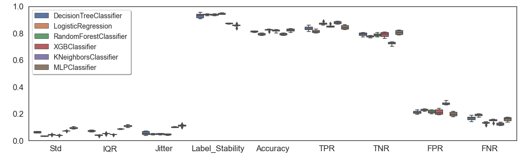
Figure 2. Statistical bias and variance metrics on folktables.

Table 3. Statistical bias-based and variance-based fairness metrics on folktables, averaged over 6 runs. RF is Random Forest, DT is Decision Tree, XGB is XGBoost, MLP is Multi-Layer Perceptron, LR is Logistic Regression and kNN is k-Nearest Neighbors

	RF	DT	XGB	MLP	LR	kNN
Accuracy Parity (sex)	-0.0793	-0.0662	-0.0656	-0.0634	-0.0618	-0.0588
Accuracy Parity (race)	-0.0057	0.0076	-0.0013	0.0015	-0.0010	0.0069
Accuracy Parity (sex&race)	-0.0756	-0.0545	-0.0597	-0.0560	-0.0587	-0.0508
Equalized Odds FPR (sex)	0.1047	0.0991	0.0592	0.0487	0.0124	0.0244
Equalized Odds FPR (race)	0.0238	0.0152	0.0135	-0.0154	-0.0069	-0.0086
Equalized Odds FPR (sex&race)	0.1278	0.1176	0.0716	0.0323	0.0056	0.0246
Statistical Parity Difference (sex)	0.1450	0.1678	0.0474	0.0293	-0.0328	0.0086
Statistical Parity Difference (race)	0.1048	0.0992	0.0596	0.0105	0.0246	0.0644
Statistical Parity Difference (sex&race)	0.1998	0.2316	0.0785	0.0205	-0.0268	0.0682
Disparate Impact (sex)	1.1351	1.1644	1.0436	1.0274	0.9705	1.0071
Disparate Impact (race)	1.0942	1.0928	1.0546	1.0097	1.0227	1.0536
Disparate Impact (sex&race)	1.1944	1.2350	1.0746	1.0195	0.9753	1.0568
IQR Parity (sex)	0.0027	-0.0045	0.0029	0.0210	0.0017	0.0110
IQR Parity (race)	-0.0016	-0.0032	0.0037	0.0109	0.0068	-0.0066
IQR Parity (sex&race)	0.0021	-0.0065	0.0072	0.0312	0.0091	0.0044
Jitter Parity (sex)	0.0153	0.0242	0.0126	0.0374	0.0035	0.0418
Jitter Parity (race)	0.0017	0.0083	0.0085	0.0158	0.0034	-0.0093
Jitter Parity (sex&race)	0.0168	0.0335	0.0213	0.0498	0.0085	0.0272
Std Parity (sex)	0.0016	-0.0028	0.0026	0.0165	0.0013	0.0091
Std Parity (race)	-0.0013	0.0008	0.0034	0.0086	0.0051	-0.0046
Std Parity (sex&race)	0.0009	-0.0014	0.0065	0.0246	0.0069	0.0047
Label Stability Ratio (sex)	0.9770	0.9641	0.9810	0.9448	0.9964	0.9394
Label Stability Ratio (race)	0.9977	0.9884	0.9880	0.9746	0.9952	1.0141
Label Stability Ratio (sex&race)	0.9754	0.9512	0.9688	0.9262	0.9892	0.9609

4.4. The Fairness-Variance-Accuracy Trade-off

Overall, as expected, ensemble models (Random Forest and XGBoost) are the most stable on all metrics and all datasets. Generally, the kNN and Decision Tree classifiers score highly on variance metrics (i.e., are the least stable). The neural network (MLP) is stable on COMPAS, but is the least stable model on folktables! This is interesting, and counter-intuitive to the general understanding of how estimator variance relates to dataset size: folktables has 20k samples, while COMPAS has only 5k samples. From a statistical bias perspective, all models perform poorly on COMPAS (no model has accuracy higher than $68\%$).

4.4.1. Folktables

The MLP classifier and Random Forest are the best performing models on folktables, with an accuracy of $82.16\%$ and $82.3\%$ respectively. Random Forest is also one of the most stable models (low Std, low IQR, low Jitter, and high Label Stability), while MLP is one of the least stable models (both MLP and kNN have high Std, IQR and Jitter, and low Label Stability).

From a fairness perspective, the MLP classifier and Logistic Regression perform the best. The Logistic Regression is not the best model on overall metrics, but has good parity on both statistical bias-based and variance-based metrics on folktables, as reported in Table 3. This is the first indication of a fairness-variance-accuracy trade-off: parity in variance and parity in statistical bias (“fairness”) comes at the cost of overall model accuracy.

Strikingly, the MLP is also a reasonably fair model — it shows low Statistical Parity Difference and Disparate Impact (close to 0 and 1, respectively), despite having low overall stability and large disparity in variance-based metrics across groups. We argue that this is a feature and not a bug, and is, once again, the fairness-variance-accuracy trade-off at play: the classifier shows a larger variation in outputs on dis than on priv, and this has a corrective effect on both the overall fairness and accuracy. Here, we are trading off stability/variance to gain fairness and accuracy.

The behavior of the Random Forest classifier also illustrates this trade-off: as mentioned previously, the Random Forest has the highest accuracy of all the models. From Table 3 we see that this classifier also shows good parity on almost all variance metrics. This, however, comes with model unfairness (large disparity in statistical bias)! On metrics that relate to model error (such as accuracy parity and equalized odds) the model is “unfair”, in the sense that it discriminates against the dis group. However, on metrics that track selection rates (such as statistical parity and disparate impact) the Random Forest classifier shows reverse discrimination, in the sense that it over-selects the dis group. Here, the model trades off fairness on the one hand for high accuracy and parity in variance on the other hand.

There is no observable consistent trend in terms of fairness or stability for the kNN and XGBoost classifiers, and perhaps their lower overall accuracy compared to other models can also be explained by a sub-optimal trade-off on the fairness-variance-accuracy spectrum.

Table 4. Statistical bias-based and variance-based fairness metrics on COMPAS, averaged over 10 runs. RF is Random Forest, DT is Decision Tree, XGB is XGBoost, MLP is Multi-Layer Perceptron, LR is Logistic Regression and kNN is k-Nearest Neighbors

	MLP	XGB	RF	LR	kNN	DT
Accuracy Parity (sex)	-0.0247	-0.1869	-0.0112	-0.0098	-0.0038	0.0035
Accuracy Parity (race)	0.0120	0.0302	0.0171	0.0085	0.0151	0.0181
Accuracy Parity (sex&race)	-0.0058	0.0163	-0.0016	-0.0031	0.0052	0.0061
Equalized Odds FPR (sex)	0.0960	0.0803	0.0846	0.0863	0.0587	0.0606
Equalized Odds FPR (race)	0.1523	0.1163	0.1188	0.1686	0.1270	0.1359
Equalized Odds FPR (sex&race)	0.2122	0.1617	0.1831	0.2206	0.1653	0.1695
Statistical Parity Difference (sex)	0.1288	0.0019	0.0974	0.0898	0.0178	0.0268
Statistical Parity Difference (race)	0.3154	0.2155	0.2211	0.3059	0.2223	0.2148
Statistical Parity Difference (sex&race)	0.3913	0.1996	0.2964	0.3519	0.2489	0.1867
Disparate Impact (sex)	1.1816	1.0021	1.1236	1.1102	1.0198	1.0287
Disparate Impact (race)	1.5180	1.2710	1.3054	1.4437	1.2899	1.2639
Disparate Impact (sex&race)	1.7199	1.2478	1.4538	1.5436	1.3396	1.2209
IQR Parity (sex)	0.0018	-0.0005	0.0028	0.0029	0.0008	0.00007
IQR Parity (race)	0.0029	0.0051	0.0024	0.0031	0.0046	0.0020
IQR Parity (sex&race)	0.0038	0.0003	0.0036	0.0051	0.0048	-0.0045
Jitter Parity (sex)	-0.0035	-0.0296	0.0005	0.0055	-0.0056	-0.0137
Jitter Parity (race)	0.0157	-0.0008	0.0116	0.0146	0.0242	0.0098
Jitter Parity (sex&race)	0.0160	-0.0395	0.0136	0.0209	0.0191	-0.0072
Std Parity (sex)	0.0014	-0.00004	0.0020	0.0021	0.0003	-0.0059
Std Parity (race)	0.0023	0.0042	0.0020	0.0023	0.0028	0.00477
Std Parity (sex&race)	0.0030	0.0010	0.0028	0.0037	0.0029	-0.00647
Label Stability Ratio (sex)	1.0069	1.0564	0.9975	0.9894	1.0104	1.0210
Label Stability Ratio (race)	0.9731	1.0052	0.9795	0.9777	0.9597	0.9894
Label Stability Ratio (sex&race)	0.9733	1.0805	0.9738	0.9667	0.9682	1.0125

4.4.2. COMPAS

As described previously, none of the models in our experiments are particularly accurate on COMPAS. As expected, we also do not find these models to be particularly fair along any of the sensitive attributes, and for any fairness metrics. XGBoost is the most accurate model, and it does show parity for a handful of the bias-based metrics (Statistical Parity Difference and Disparate Impact, both along the lines of sex) and variance-based metrics (for IQR parity, Jitter parity, and Label stability ratio). For a classifier that has low overall accuracy, stability (low variance) and uniform stability (parity in variance) negates any potentially corrective effect estimator variance could have had, and results in model unfairness.

Interestingly, the Decision Tree is the most “fair” model on COMPAS — it is close to having parity in accuracy across all groups and has the best parity in bias-based metrics for intersectional groups. Further, unlike the XGBoost classifier on COMPAS, the Decision Tree is far from having parity in variance, and it, in fact has higher variance on the priv group. Here, we see the corrective effect of estimator variance on the “fairness” of an inaccurate model: the Decision Tree has low accuracy — even as compared to the other poorly performing models — but its disparity in variance seems to improve the parity in statistical bias-based measures.

4.5. Comparing variance metrics

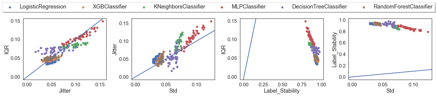
Figure 4. folktables (20k samples): Relationship between different variance metrics. Y=X line is plotted in blue

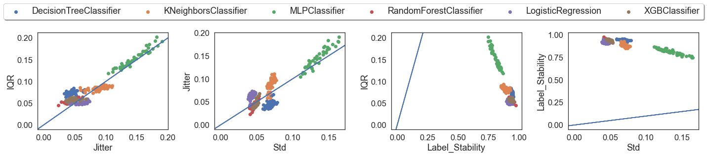
Figure 5. folktables (5k samples): Relationship between different variance metrics. Y=X line is plotted in blue

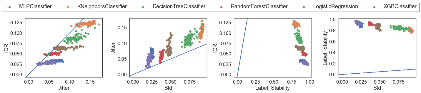
Figure 6. COMPAS (5k samples): Relationship between different variance metrics. Y=X line is plotted in blue

In our last set of experiments, we examined two families of complimentary variance metrics: (1) Standard deviation (Std) and Inter-Quantile Range (IQR) track the spread of the predicted probabilities, while (2) Jitter and Label Stability track how often the predicted label flips. We compare how “good” (i.e., informative) these different measures of estimator variance are in Figures 4 and 5 for folktables, and in Figure 6 for COMPAS.

The behavior of variance metrics seems to be both model-specific and-dataset specific. The MLP classifier (shown in red dots in Figure 4 and in green dots in Figure 5) falls approximately on the $Y=X$ line (plotted in blue in both figures). This means that IQR, Jitter and Std are highly correlated, and so can be used interchangeably for this model. Extending our earlier discussion of the instability of the MLP classifier on folktables: we see high instability in both the model that was trained on 5k samples (Figure 4) and in the model that was trained on 20k samples (Figure  5). As expected, estimator variance decreases as the sample size increases: the MLP classifier trained with 20k and 5k samples has a maximum (worst-case) IQR of approximately 0.15 and 0.20 respectively.

We see interesting trends in estimator variance on the COMPAS dataset: in Figure 6, variance metrics reported for different model types forms clusters that are almost constant along one dimension. For the same value of IQR, models have a range of values of Jitter (left-most subplot), and for the same value of Std, models have a range of values for Jitter (second plot from the left). We do not observe this behavior when considering Label Stability: the metrics of different models do form clusters, but they do not stay constant along one dimension. This suggests that, while we may be tempted to treat them interchangeably, we do need to look at them as a set, since reporting them on different benchmark datasets (such as COMPAS here) could lead to some metrics appearing to be redundant, despite being informative in a different context (such as on folktables in Figure 4 and 5).

5. conclusions and Future Work

In this work we attempted to clarify the desiderata of fairness and stability, by asking the question: “Is estimator variance a friend or a foe?”. In answering this question we uncovered the fairness-variance-accuracy trade-off, an enrichment of the classically understood fairness-accuracy and accuracy-robustness trade-offs. We empirically demonstrated contexts in which large estimator variance, as well as large disparity in estimator variance, can have a corrective effect on both model accuracy and fairness, but we also identified scenarios in which variance fails to help. We hope that our work will usher in a new paradigm of fairness-enhancing interventions that go beyond the classic fairness-accuracy dichotomy (Chouldechova and Roth, 2020). For instance, there is interesting future work to be done to exploit large noise variance on protected groups with improved fairness and accuracy through this fairness-variance-accuracy trichotomy. Furthermore, our insights on the effect of estimator variance could help guide model selection in cases when several models are equally “fair” or equally accurate.

Our work also comes with important limitations: Lum et al. (2022) highlight statistical errors in the measurement of different performance metrics, and the statistical procedures used to compute estimator variance in this study also suffer from the same shortcomings. There are also interesting statistical questions around the variance of these variance estimates — specially in social contexts where it is widely believed that noise variance tracks protected attributes (Kappelhof, 2017; Schelter et al., 2019) — which we leave for future work.

Fairness is not a purely technical or statistical concept, but rather a normative and philosophical one. The major contributions of this work (methods, results and analysis) are purely technical, and are based on a popular technical definition of “fairness” as the parity in statistical bias. This is of course a limiting view, and one that should be regarded within a broader socio-legal-political view of fairness.

One of the contributions of our work is the Virny software library. We envision several enhancements to our software library. Firstly, we would like to support other sampling-during-inference techniques for variance estimation beyond the simple Bootstrap, such as the Jackknife (Miller, 1974), as well as combinations of Bootstrap and Jackknife (Barber et al., 2021; Kim et al., 2020; Efron, 1992). We would also like to evaluate Conformal Prediction methods (Vovk et al., 2017; Shafer and Vovk, 2008; Angelopoulos and Bates, 2021) for quantifying and correcting model instability. Specifically, it would be interesting to compare the insights from the variance metrics analyzed in this study with insights from the coverage and interval widths on different protected groups of conformal methods.

References

- (1)
- Angelopoulos and Bates (2021) Anastasios N Angelopoulos and Stephen Bates. 2021. A gentle introduction to conformal prediction and distribution-free uncertainty quantification. arXiv preprint arXiv:2107.07511 (2021).
- Angwin et al. (2016) Julia Angwin, Jeff Larson, Surya Mattu, and Lauren Kirchner. 2016. Machine Bias. ProPublica (2016).
- Barber et al. (2021) Rina Foygel Barber, Emmanuel J Candes, Aaditya Ramdas, and Ryan J Tibshirani. 2021. Predictive inference with the jackknife+. The Annals of Statistics 49, 1 (2021), 486–507.
- Bellamy et al. (2018) Rachel KE Bellamy, Kuntal Dey, Michael Hind, Samuel C Hoffman, Stephanie Houde, Kalapriya Kannan, Pranay Lohia, Jacquelyn Martino, Sameep Mehta, Aleksandra Mojsilovic, et al. 2018. AI Fairness 360: An extensible toolkit for detecting, understanding, and mitigating unwanted algorithmic bias. arXiv preprint arXiv:1810.01943 (2018).
- Bird et al. (2020) Sarah Bird, Miro Dudík, Richard Edgar, Brandon Horn, Roman Lutz, Vanessa Milan, Mehrnoosh Sameki, Hanna Wallach, and Kathleen Walker. 2020. Fairlearn: A toolkit for assessing and improving fairness in AI. Microsoft, Tech. Rep. MSR-TR-2020-32 (2020).
- Chouldechova (2017) Alexandra Chouldechova. 2017. Fair Prediction with Disparate Impact: A Study of Bias in Recidivism Prediction Instruments. Big Data 5, 2 (2017), 153–163. https://doi.org/10.1089/big.2016.0047
- Chouldechova and Roth (2020) Alexandra Chouldechova and Aaron Roth. 2020. A snapshot of the frontiers of fairness in machine learning. Commun. ACM 63, 5 (2020), 82–89. https://doi.org/10.1145/3376898
- Darling and Stracuzzi (2018) Michael C. Darling and David J. Stracuzzi. 2018. Toward Uncertainty Quantification for Supervised Classification.
- Ding et al. (2021) Frances Ding, Moritz Hardt, John Miller, and Ludwig Schmidt. 2021. Retiring Adult: New Datasets for Fair Machine Learning. In Advances in Neural Information Processing Systems 34: Annual Conference on Neural Information Processing Systems 2021, NeurIPS 2021, December 6-14, 2021, virtual, Marc’Aurelio Ranzato, Alina Beygelzimer, Yann N. Dauphin, Percy Liang, and Jennifer Wortman Vaughan (Eds.). 6478–6490. https://proceedings.neurips.cc/paper/2021/hash/32e54441e6382a7fbacbbbaf3c450059-Abstract.html
- Dwork (2011) Cynthia Dwork. 2011. A firm foundation for private data analysis. Commun. ACM 54, 1 (2011), 86–95. https://doi.org/10.1145/1866739.1866758
- Dwork et al. (2012) Cynthia Dwork, Moritz Hardt, Toniann Pitassi, Omer Reingold, and Richard S. Zemel. 2012. Fairness through awareness. In Innovations in Theoretical Computer Science 2012, Cambridge, MA, USA, January 8-10, 2012, Shafi Goldwasser (Ed.). ACM, 214–226. https://doi.org/10.1145/2090236.2090255
- Efron (1992) Bradley Efron. 1992. Jackknife‐After‐Bootstrap Standard Errors and Influence Functions. Journal of the royal statistical society series b-methodological 54 (1992), 83–111.
- Efron and Tibshirani (1994) Bradley Efron and Robert J Tibshirani. 1994. An introduction to the bootstrap. CRC press.
- Friedler et al. (2019) Sorelle A Friedler, Carlos Scheidegger, Suresh Venkatasubramanian, Sonam Choudhary, Evan P Hamilton, and Derek Roth. 2019. A comparative study of fairness-enhancing interventions in machine learning. In Proceedings of the conference on fairness, accountability, and transparency. 329–338.
- Han et al. (2022) Xudong Han, Aili Shen, Yitong Li, Lea Frermann, Timothy Baldwin, and Trevor Cohn. 2022. fairlib: A unified framework for assessing and improving classification fairness. arXiv preprint arXiv:2205.01876 (2022).
- Hardt et al. (2016) Moritz Hardt, Eric Price, and Nati Srebro. 2016. Equality of Opportunity in Supervised Learning. In Advances in Neural Information Processing Systems 29: Annual Conference on Neural Information Processing Systems 2016, December 5-10, 2016, Barcelona, Spain, Daniel D. Lee, Masashi Sugiyama, Ulrike von Luxburg, Isabelle Guyon, and Roman Garnett (Eds.). 3315–3323. https://proceedings.neurips.cc/paper/2016/hash/9d2682367c3935defcb1f9e247a97c0d-Abstract.html
- Huang and Vishnoi (2019) Lingxiao Huang and Nisheeth Vishnoi. 2019. Stable and fair classification. In International Conference on Machine Learning. PMLR, 2879–2890.
- Kappelhof (2017) Joost Kappelhof. 2017. Total Survey Error in Practice. Chapter Survey Research and the Quality of Survey Data Among Ethnic Minorities.
- Kim et al. (2020) Byol Kim, Chen Xu, and Rina Barber. 2020. Predictive inference is free with the jackknife+-after-bootstrap. Advances in Neural Information Processing Systems 33 (2020), 4138–4149.
- Kleinberg et al. (2017) Jon M. Kleinberg, Sendhil Mullainathan, and Manish Raghavan. 2017. Inherent Trade-Offs in the Fair Determination of Risk Scores. In 8th Innovations in Theoretical Computer Science Conference, ITCS 2017, January 9-11, 2017, Berkeley, CA, USA (LIPIcs, Vol. 67), Christos H. Papadimitriou (Ed.). Schloss Dagstuhl - Leibniz-Zentrum für Informatik, 43:1–43:23. https://doi.org/10.4230/LIPIcs.ITCS.2017.43
- Liu et al. (2022a) Huiting Liu, Siddharth Patwardhan, Peter Grasch, Sachin Agarwal, et al. 2022a. Model Stability with Continuous Data Updates. arXiv preprint arXiv:2201.05692 (2022).
- Liu et al. (2022b) Huiting Liu, Siddharth Patwardhan, Peter Grasch, Sachin Agarwal, et al. 2022b. Model Stability with Continuous Data Updates. arXiv preprint arXiv:2201.05692 (2022).
- Lum et al. (2022) Kristian Lum, Yunfeng Zhang, and Amanda Bower. 2022. De-Biasing “Bias” Measurement (FAccT ’22). Association for Computing Machinery, New York, NY, USA, 379–389. https://doi.org/10.1145/3531146.3533105
- Milani Fard et al. (2016) Mahdi Milani Fard, Quentin Cormier, Kevin Canini, and Maya Gupta. 2016. Launch and iterate: Reducing prediction churn. Advances in Neural Information Processing Systems 29 (2016).
- Miller (1974) Rupert G. Miller. 1974. The Jackknife–A Review. Biometrika 61, 1 (1974), 1–15. http://www.jstor.org/stable/2334280
- Saleiro et al. (2018) Pedro Saleiro, Benedict Kuester, Loren Hinkson, Jesse London, Abby Stevens, Ari Anisfeld, Kit T Rodolfa, and Rayid Ghani. 2018. Aequitas: A bias and fairness audit toolkit. arXiv preprint arXiv:1811.05577 (2018).
- Schelter et al. (2019) Sebastian Schelter, Yuxuan He, Jatin Khilnani, and Julia Stoyanovich. 2019. Fairprep: Promoting data to a first-class citizen in studies on fairness-enhancing interventions. EDBT (2019).
- Shafer and Vovk (2008) Glenn Shafer and Vladimir Vovk. 2008. A Tutorial on Conformal Prediction. Journal of Machine Learning Research 9, 3 (2008).
- Vasudevan and Kenthapadi (2020) Sriram Vasudevan and Krishnaram Kenthapadi. 2020. Lift: A scalable framework for measuring fairness in ml applications. In Proceedings of the 29th ACM international conference on information & knowledge management. 2773–2780.
- Vovk et al. (2017) Vladimir Vovk, Jieli Shen, Valery Manokhin, and Min-ge Xie. 2017. Nonparametric predictive distributions based on conformal prediction. In Conformal and Probabilistic Prediction and Applications. PMLR, 82–102.