RIS-aided Localization under Pixel Failures

Abstract

Reconfigurable intelligent surfaces (RISs) hold great potential as one of the key technological enablers for beyond-5G wireless networks, improving localization and communication performance under line-of-sight (LoS) blockage conditions. However, hardware imperfections might cause RIS elements to become faulty, a problem referred to as pixel failures, which can constitute a major showstopper especially for localization. In this paper, we investigate the problem of RIS-aided localization of a user equipment (UE) under LoS blockage in the presence of RIS pixel failures, considering the challenging single-input single-output (SISO) scenario. We first explore the impact of such failures on accuracy through misspecified Cramér-Rao bound (MCRB) analysis, which reveals severe performance loss with even a small percentage of pixel failures. To remedy this issue, we develop two strategies for joint localization and failure diagnosis (JLFD) to detect failing pixels while simultaneously locating the UE with high accuracy. The first strategy relies on $\ell_{1}$-regularization through exploitation of failure sparsity. The second strategy detects the failures one-by-one by solving a multiple hypothesis testing problem at each iteration, successively enhancing localization and diagnosis accuracy. Simulation results show significant performance improvements of the proposed JLFD algorithms over the conventional failure-agnostic benchmark, enabling successful recovery of failure-induced performance degradations.

I Introduction

I-A Background and Motivation

RIS are envisaged as a key enabling technology towards 6G to reduce the vulnerability of mmWave and sub-THz systems to signal blockages, providing improved communication rate and coverage [1, 2, 3]. Through their dynamic ability to engineer the propagation environment, reconfigurable intelligent surfaces can be optimized in terms of various performance metrics, such as energy efficiency [4, 5] and sum-rate [6, 7]. While a great deal of papers has been devoted to RIS for communication, especially for overcoming line-of-sight (LoS) blockages [1, 8], RISs enjoy several properties that make them attractive for localization as well [9, 10]. The large aperture of RISs enables high resolution in angle-of-arrival (AoA) and angle-of-departure (AoD) estimation, while their functioning over large bandwidths supports high delay resolution (in addition to high data rates) [11]. When user equipments are close to the RIS, wavefront curvature (also known as near-field (NF)) allows direct relative localization, even when the LoS between the UE and base station (BS) is blocked [12, 13, 14]. When the RIS has a known location and orientation, this relative location can be transformed into global coordinates, effectively rendering the RIS into an additional analog BS [11].

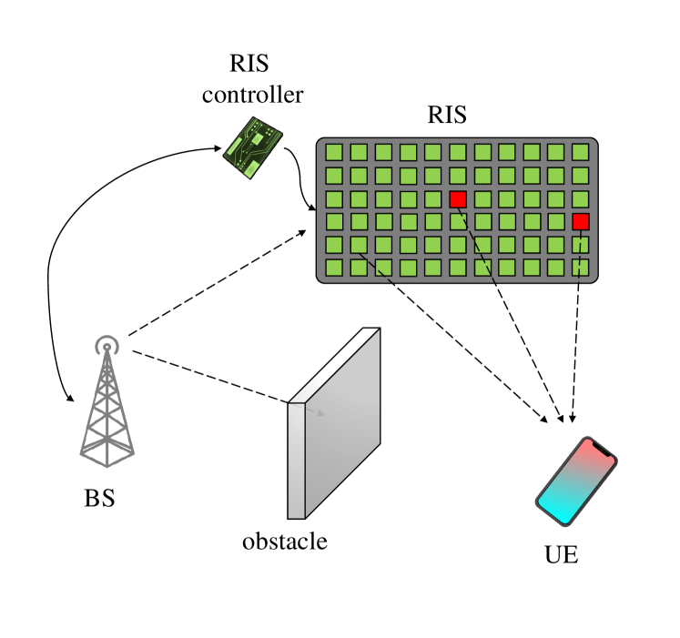
Figure 1: Scenario under consideration, comprising a single-antenna BS, a single-antenna UE, and an RIS. The LoS path between the BS and the UE is blocked, while the UE lies in the near-field of the RIS. The colors on the RIS elements indicate the status of different pixels (green means properly functioning element, while red indicates failing pixel). The goal is to localize the UE in 3D under RIS pixel failures using a set of scalar baseband observations, which leads to the problem of joint localization and RIS diagnosis.

In light of the above observations, a number of studies has recently investigated RIS for NF localization [15, 12, 16, 14, 13, 17, 18, 19]. In [15], performance bounds and a practical method for narrowband NF localization of a transmitter with an RIS acting as a lens has been presented. The studies in [16, 14] consider a more conventional setup including a reflective RIS and a BS to evaluate [16] and mitigate [14] the impact of phase-dependent amplitude variations of the RIS elements on NF localization accuracy. Taking into account the scatterers in the links from BS to RIS and from RIS to UE, [13] employs compressive sampling and optimized RIS configurations to achieve high accuracy. Moreover, RIS phase profile optimization for localization in NF has been proposed in [17] based on a combination of positional and derivative beams, which reveals considerable improvements over standard positional beams. The work in [18] tackles a similar problem for a linear RIS. Furthermore, direct and two-step estimators for LoS/ non-line-of-sight (NLoS) NF localization using orthogonal frequency-division multiplexing (OFDM) transmission have been developed in [12] for a stripe-like RIS, where sub-cm level accuracy has been demonstrated. Finally, the study in [19] derives the theoretical limits on NF localization with hybrid RIS and determines localization-optimal RIS configurations.

I-B Related Work on Failures

An important consideration in a practical RIS, which may comprise several hundreds of unit elements (or pixels), is that individual elements may fail. This problem also exists in the array processing literature. In [20], antenna array diagnosis has been studied in a standard mmWave setup without a RIS and several compressive sensing based techniques have been proposed to identify the faulty antenna elements and the resulting amplitude and phase distortions. The AoA estimation problem under element failures has been considered in [21], where the diagnosis of faulty elements is formulated as a Toeplitz matrix reconstruction problem. Recently, several papers investigate RIS element failures in mmWave communications [22, 23]. In [22], the authors present different types of pixel errors (e.g., stuck at state, out of state, etc.) and their spatial distribution (independent, clustered, etc.). The paper also explores the effect of pixel errors on the radiation pattern through simulation analysis. The study in [23] establishes a failure model to specify the amplitude and phase shift of faulty elements and proposes diagnostic methods by exploiting the sparsity property of failures. In [24], joint phase error calibration and channel estimation algorithm has been proposed to deal with RIS phase offsets induced by hardware impairments. Moreover, [25] evaluates the impact of failures and phase quantization errors on the signal-to-noise ratio (SNR) of RIS-aided high-mobility vehicular communications.

In addition to element failures resulting from internal hardware imperfections, RIS element blockages due to external environmental effects such as dust, rain and ice have been studied in recent works [26, 27]. In [26], blockages at both the BS and RIS are considered and an iterative algorithm is proposed to jointly estimate the blockage coefficients of the BS and RIS. In [27], the authors propose a two-stage algorithm for joint RIS diagnosis and channel estimation in a RIS-aided mmWave MIMO system. Despite a considerable amount of research on pixel failures in RIS-aided communications, to the best of the authors’ knowledge, no study has been performed to tackle the problem of RIS-aided localization in the presence of pixel failures. Hence, two fundamental questions arise that remain unanswered so far: (i) how severe can the impact of RIS element failures be on the localization accuracy?, and (ii) is it possible to perform RIS diagnosis and UE localization simultaneously?

I-C Contributions

In this paper, we address both of these knowledge gaps, and perform an in-depth analysis of RIS pixel failures in terms of achievable localization accuracy. We also propose novel algorithms to identify faulty pixels and mitigate their impact on localization, even when the UE location is a-priori unknown. The main contributions can be listed as follows:

• Localization under RIS Pixel Failures: For the first time, we investigate the problem of RIS-aided localization under pixel failures by adopting a practical failure model based on biases in individual failing elements [22, 23]. We consider a narrowband geometric near-field scenario where a single-antenna UE estimates its location using downlink signals by a single-antenna BS in the presence of a RIS with LoS blockage. The biases can change the resulting RIS phase profiles and lead to a challenging problem of joint localization and failure diagnosis (JLFD).

• Impact of Failures on Localization Accuracy: We carry out a theoretical analysis on how detrimental RIS pixel failures can be for RIS-aided localization. To quantify the effect of failures on the localization performance, we conduct a misspecified Cramér-Rao bound (MCRB) analysis [28] under mismatch between a true model with pixel failures and an assumed model without failures (i.e., the UE is unaware of failures), which reveals fundamental insights on when such failures can induce severe degradations in localization accuracy (i.e., SNR regimes, number of failing elements, etc.).

• Sparsity-Inspired Joint Localization and Failure Diagnosis Algorithms: By exploiting the sparsity of failures, we propose two algorithms to tackle the JLFD problem, which involves joint estimation of the UE location and the locations and failure coefficients (i.e., biases) of the faulty elements. The first one, called $\ell_{1}$-JLFD, is based on an $\ell_{1}$-regularization approach that estimates the failure mask and the UE location using an alternating optimization strategy. The second algorithm, called Successive-JLFD, explicitly considers the statistics of pixel failures and solves the resulting hybrid ML/MAP estimation problem in an iterative manner, in a spirit similar to that of OMP based sparse channel estimation algorithms [29, 30, 31]. In particular, Successive-JLFD detects the failures one-by-one at each iteration and proceeds by canceling out their impact on the subsequent iterations, progressively improving the performance of localization and failure mask estimation.

Additionally, simulation results showcase the sensitivity of localization performance to pixel failures, which indicates the need for powerful methods to counteract such impairments. In the challenging single-input single-output (SISO) RIS scenario under consideration, the proposed JLFD algorithms are shown to recover performance losses resulting from pixel failures and achieve accuracy levels very close to theoretical limits corresponding to the case with known failure mask (i.e., perfectly calibrated/diagnosed RIS).

II System Model and Problem Description

In this section, we describe the system geometry and the signal model, introduce the RIS pixel failure model, and formulate the problem of localization under pixel failures.

II-A Geometry and Signal Model

Consider an RIS-aided downlink (DL) localization scenario consisting of a single-antenna BS, an $N$-element RIS, and a single-antenna UE, as shown in Fig. 1. The BS is located at a known position $\bm{p}_{\text{BS}}\in\mathbb{R}^{3}$, while $\bm{p}_{\text{RIS}}\in\mathbb{R}^{3}$ denotes the known center of the RIS and $\bm{p}_{n}\in\mathbb{R}^{3}$ represents the known location of the $n$-th RIS element for $1\leq n\leq N$. The UE has an unknown location $\bm{p}\in\mathbb{R}^{3}$, which needs to be estimated. In this scenario, the UE is assumed to lie in the Fresnel (radiative) NF region of the RIS [32, 33, 34], i.e.,

$$0.62\sqrt{\frac{D^{3}}{\lambda}}\leq d\leq\frac{2D^{2}}{\lambda}\leavevmode\nobreak\ ,$$ (1)

where $\lambda$, $D$ and $d$ denote, respectively, the carrier wavelength, the RIS aperture size (i.e., the largest distance between any two RIS elements) and the distance to the RIS.

For DL communications, the BS transmits narrowband pilots $\bm{s}=[s_{1}\ \cdots\ s_{T}]^{\mathsf{T}}\in\mathbb{C}^{T\times 1}$ over $T$ transmission instances under an average power constraint $\mathbb{E}\left\{\lvert s_{t}\rvert^{2}\right\}=E_{s}$. To motivate the deployment of a RIS, we assume that the LoS path between the BS and the UE is blocked [1, 8], e.g., due to buildings, cars or trees. In addition, it is assumed that no uncontrolled multipath (i.e., those paths induced by scattering/reflection off the passive objects in the environment) exists. Then, the DL communications occur only through the RIS and the DL signal received by the UE at transmission $t$ is given by

$$y_{t}=\alpha\,\bm{a}^{\mathsf{T}}(\bm{p})\mathrm{diag}(\bm{\gamma}_{t})\bm{a}(\bm{p}_{\text{BS}})s_{t}+n_{t}\,,$$ (2)

where $\alpha$ is the unknown channel gain, $\bm{\gamma}_{t}\in\mathbb{C}^{N\times 1}$ is the RIS phase profile at transmission $t$, and $n_{t}$ is zero-mean additive white Gaussian noise with variance $N_{0}/2$ per real dimension. Moreover, $\bm{a}(\bm{p})\in\mathbb{C}^{N\times 1}$ denotes the NF RIS steering vector for a given position $\bm{p}$, which can be expressed by taking the RIS center $\bm{p}_{\text{RIS}}$ to be the reference point as [36], [34]

$$[\bm{a}(\bm{p})]_{n}=\exp\left(-j\frac{2\pi}{\lambda}\left(\left\lVert\bm{p}-\bm{p}_{n}\right\rVert-\left\lVert\bm{p}-\bm{p}_{\text{RIS}}\right\rVert\right)\right)$$ (3)

for $n\in\{1,\ldots,N\}$. For convenience, let us define $\bm{y}=[y_{1}\,\cdots\,y_{T}]^{\mathsf{T}}$, $\bm{b}(\bm{p})=\bm{a}(\bm{p})\odot\bm{a}(\bm{p}_{\text{BS}})$, $\bm{\Gamma}=[\bm{\gamma}_{1}\,\cdots\,\bm{\gamma}_{T}]\in\mathbb{C}^{N\times T}$, $\bm{S}=\mathrm{diag}(s_{1},\ldots,s_{T})$ and $\bm{n}=[n_{1}\,\cdots\,n_{T}]^{\mathsf{T}}$, with $\odot$ denoting the Hadamard (element-wise) product. Then, the observations in (2) can be written compactly as

$$\bm{y}=\alpha\bm{S}\bm{\Gamma}^{\mathsf{T}}\bm{b}(\bm{p})+\bm{n}\leavevmode\nobreak\ ,$$ (4)

where $\bm{n}\sim{\mathcal{CN}}({{\bm{0}}},\allowbreak N_{0}{\bm{\mathrm{I}}})$.

II-B RIS Pixel Failure Model

To model RIS pixel/element failures, we consider biases in individual RIS elements, where the element switches to a valid, biased state with a certain distance from the desired state due to bit-flipping or external biases [22, 23]. Under such element failures, the RIS phase profile $\bm{\gamma}_{t}$ in (2) can be modeled as

$$\bm{\gamma}_{t}=\bm{\phi}_{t}\odot\bm{m}\,,$$ (5)

where $\bm{\phi}_{t}\in\mathbb{C}^{N\times 1}$ represents the configurable RIS weights under the designer’s control, and $\bm{m}=[m_{1}\,\cdots\,m_{N}]\in\mathbb{C}^{N\times 1}$ denotes the unknown failure mask quantifying the effect of faulty elements, which can be defined as [20, 23]

$$m_{n} =\begin{cases}\zeta_{n},&{\textrm{if the ${n^{\rm{th}}}$ RIS element is faulty (biased)}}\\ 1,&\textrm{if the ${n^{\rm{th}}}$ RIS element is properly functioning}\end{cases}.$$ (6)

In (6), $\zeta_{n}=\kappa_{n}e^{j\psi_{n}}$ denotes the failure related complex response of the $n$-th element, with $0<\kappa_{n}\leq 1$ and $0\leq\psi_{n}<2\pi$ representing the resulting attenuation and phase shift, respectively.

We assume a stochastic failure model where each RIS element fails independently from each other with the probability $p_{{\rm{fail}}}$. In addition, when the ${n^{\rm{th}}}$ pixel fails, its complex response $\zeta_{n}$ follows the distribution $\kappa_{n}\sim\mathcal{U}(0,1)$ and $\psi_{n}\sim\mathcal{U}(-\pi,\pi)$ [23]. Formally, each element $m_{n}$ of the failure mask in (6) can be expressed as [37]

$$m_{n}=c_{n}\zeta_{n}+1-c_{n}\leavevmode\nobreak\ ,$$ (7)

where the binary variable $c_{n}\in\{0,1\}$ specifies the absence/presence of failure, with $c_{n}\sim{{\rm{Ber}}}(p_{{\rm{fail}}})$, and $\zeta_{n}\in\mathbb{C}$ corresponds to the complex amplitude of the failing element in case of failure. According to (7), when $c_{n}=0$ (i.e., no failure), we have $m_{n}=1$, while $c_{n}=1$ (i.e., failure) sets $m_{n}=\zeta_{n}$, in compliance with (6). Hence, $m_{n}$ has a spike-and-slab prior [37, 38, 39], given by

$$f_{m_{n}}(m_{n})=(1-p_{{\rm{fail}}})\delta(m_{n}-1)+p_{{\rm{fail}}}f_{\zeta_{n}}(m_{n})\leavevmode\nobreak\ ,$$ (8)

where $m_{n}$ attains the “spike” value $1$ if the ${n^{\rm{th}}}$ element is functioning and is drawn from the “slab” probability density function (pdf) $f_{\zeta_{n}}(m)$ in case of failure (see App. A for the derivation of $f_{\zeta_{n}}(m)$).

Defining $\bm{\Phi}=[\bm{\phi}_{1}\,\cdots\,\bm{\phi}_{T}]\in\mathbb{C}^{N\times T}$ and denoting by ${{\bm{1}}}$ an all-ones vector, the RIS phase profiles $\bm{\Gamma}$ in (4) can be expressed under the failure model (5) as

$$\bm{\Gamma}=\bm{\Phi}\odot\bm{m}{{\bm{1}}}^{\mathsf{T}}\leavevmode\nobreak\ ,$$ (9)

where the pdf of the failure mask can be written using (8) and under the assumption of independently failing elements as

$$f_{\bm{m}}(\bm{m})=\prod_{n=1}^{N}f_{m_{n}}(m_{n})\leavevmode\nobreak\ .$$ (10)

With pixel failures in (9), the observation model (4) becomes

$$\bm{y}=\alpha\bm{S}\left(\bm{\Phi}^{\mathsf{T}}\odot{{\bm{1}}}\bm{m}^{\mathsf{T}}\right)\bm{b}(\bm{p})+\bm{n}\leavevmode\nobreak\ .$$ (11)

II-C Problem Description for Joint Localization and Failure Diagnosis

Given the observations $\bm{y}$ in (11) and the prior distribution of the failure mask $\bm{m}$ in (10), the problem of joint localization and RIS failure diagnosis is to estimate the UE position $\bm{p}$, the channel gain $\alpha$ and the failure mask $\bm{m}$. To tackle this problem, we first characterize lower bounds on localization accuracy in the presence of pixel failures in Sec. III, with the aim to evaluate performance losses due to such impairments. In Sec. IV, we formulate the problem in a mathematically rigorous manner and propose two algorithms to solve it, followed by their complexity analysis in Sec. V.

III Localization Performance Evaluation under Pixel Failures

In this section, we derive theoretical limits on localization in the presence of pixel failures under varying levels of knowledge regarding the failing pixels. To this end, we resort to the MCRB [28] as a tool to assess degradation in localization performance due to mismatch between the ideal/assumed model with no failures and the true model with pixel failures. In addition, we employ standard Cramér-Rao bound (CRB), as well, to evaluate theoretical performance under perfect knowledge of failing pixel locations and perfect/imperfect knowledge of associated complex coefficients.

III-A MCRB Analysis under Pixel Failures

In this part, we quantify localization performance for the case where the UE is unaware of pixel failures and therefore estimates its location by assuming that all pixels are functioning (i.e., $\bm{m}={{\bm{1}}}$ in (11)). We leverage the MCRB analysis to characterize theoretical limits on localization accuracy under the aforementioned conditions [28, 14].

III-A1 True and Assumed Models

We first describe the true and assumed models in the presence of pixel failures.

True Model

According to the MCRB terminology [28, 40], the true model is given by (11), i.e.,

$$\bm{y}=\macc@depth\char 1\relax\frozen@everymath{\macc@group}\macc@set@skewchar\macc@nested@a 111{\alpha}\bm{S}\left(\bm{\Phi}^{\mathsf{T}}\odot{{\bm{1}}}\bm{m}^{\mathsf{T}}\right)\bm{b}(\macc@depth\char 1\relax\frozen@everymath{\macc@group}\macc@set@skewchar\macc@nested@a 111{\bm{p}})+\bm{n}\leavevmode\nobreak\$$

where $\macc@depth\char 1\relax\frozen@everymath{\macc@group}\macc@set@skewchar\macc@nested@a 111{\alpha}$ and $\macc@depth\char 1\relax\frozen@everymath{\macc@group}\macc@set@skewchar\macc@nested@a 111{\bm{p}}$ denote the true values of the unknown parameters $\alpha$ and $\bm{p}$, respectively. For a given failure mask $\bm{m}$, the pdf of the true model in (III-A1) can be written as

$$p(\bm{y})=\frac{1}{(\pi N_{0})^{T}}\exp\left\{-\frac{\left\lVert\bm{y}-\bm{\mu}\right\rVert^{2}}{N_{0}}\right\}\leavevmode\nobreak\ ,$$ (12)

where $\bm{\mu}\triangleq\macc@depth\char 1\relax\frozen@everymath{\macc@group}\macc@set@skewchar\macc@nested@a 111{\alpha}\bm{S}\left(\bm{\Phi}^{\mathsf{T}}\odot{{\bm{1}}}\bm{m}^{\mathsf{T}}\right)\bm{b}(\macc@depth\char 1\relax\frozen@everymath{\macc@group}\macc@set@skewchar\macc@nested@a 111{\bm{p}})\in\mathbb{C}^{T\times 1}$.

Assumed Model

For the assumed model, we consider an ideal RIS without pixel failures (i.e., $\bm{m}={{\bm{1}}}$ in (11)), leading to

$$\bm{y}=\alpha\bm{S}\bm{\Phi}^{\mathsf{T}}\bm{b}(\bm{p})+\bm{n}\leavevmode\nobreak\ ,$$ (13)

in which case the misspecified parametric pdf is obtained as [28]

$$\widetilde{p}(\bm{y}\lvert\bm{\eta})=\frac{1}{(\pi N_{0})^{T}}\exp\left\{-\frac{\left\lVert\bm{y}-\widetilde{\bm{\mu}}(\bm{\eta})\right\rVert^{2}}{N_{0}}\right\}\leavevmode\nobreak\ ,$$ (14)

where $\bm{\eta}=\left[\alpha_{\rm{R}},\alpha_{\rm{I}},\bm{p}^{\mathsf{T}}\right]^{\mathsf{T}}$ represents the unknown parameters, $\alpha_{\rm{R}}\triangleq\Re\left\{\alpha\right\}$, $\alpha_{\rm{I}}\triangleq\Im\left\{\alpha\right\}$ and $\widetilde{\bm{\mu}}(\bm{\eta})\triangleq\alpha\bm{S}\bm{\Phi}^{\mathsf{T}}\bm{b}(\bm{p})\in\mathbb{C}^{T\times 1}$.

III-A2 Pseudo-True Parameter

The pseudo-true parameter is used in the MCRB derivation and is defined as [28]

$$\bm{\eta}_{0}=\arg\min_{\bm{\eta}}\leavevmode\nobreak\ \mathcal{D}\left(p(\bm{y})\leavevmode\nobreak\ \|\leavevmode\nobreak\ \widetilde{p}(\bm{y}\lvert\bm{\eta})\right)\leavevmode\nobreak\ ,$$ (15)

which minimizes the Kullback-Leibler (KL) divergence $\mathcal{D}\left(p(\bm{y})\leavevmode\nobreak\ \|\leavevmode\nobreak\ \widetilde{p}(\bm{y}\lvert\bm{\eta})\right)$ between the true and assumed pdfs. In (15), $\bm{\eta}_{0}$ can be found using [14, Lemma 1].

III-A3 MCRB and LB

The covariance matrix of any misspecified-unbiased (MS-unbiased) estimator of $\bm{\eta}_{0}$ can be lower-bounded by the MCRB matrix [28]:

$$\mathbb{E}_{p}\{(\widehat{\bm{\eta}}(\bm{y})-\bm{\eta}_{0})(\widehat{\bm{\eta}}(\bm{y})-\bm{\eta}_{0})^{\mathsf{T}}\}\succeq{\rm{MCRB}}(\bm{\eta}_{0})\leavevmode\nobreak\ ,$$ (16)

where $\mathbb{E}_{p}\left\{\cdot\right\}$ represents the expectation over the true pdf in (12) and $\widehat{\bm{\eta}}(\bm{y})$ denotes an MS-unbiased estimator of $\bm{\eta}_{0}$ based on the misspecified model (13), meaning that $\mathbb{E}_{p}\left\{\widehat{\bm{\eta}}(\bm{y})\right\}=\bm{\eta}_{0}$. Hereafter, $\widehat{\bm{\eta}}(\bm{y})$ will be referred to as the failure-agnostic estimator and employed as a benchmark in performance evaluations in Sec. VI. The MCRB matrix in (16) is given by

$${\rm{MCRB}}(\bm{\eta}_{0})=\bm{A}_{\bm{\eta}_{0}}^{-1}\bm{B}_{\bm{\eta}_{0}}\bm{A}_{\bm{\eta}_{0}}^{-1}\in\mathbb{R}^{5\times 5}\leavevmode\nobreak\ ,$$ (17)

where $\bm{A}_{\bm{\eta}_{0}}\in\mathbb{R}^{5\times 5}$ and $\bm{B}_{\bm{\eta}_{0}}\in\mathbb{R}^{5\times 5}$ are defined as [28, 14]

$$[\bm{A}_{\bm{\eta}_{0}}]_{i,j} =\mathbb{E}_{p}\left\{\frac{\partial^{2}}{\partial\eta_{i}\partial\eta_{j}}\log\widetilde{p}(\bm{y}\lvert\bm{\eta})\Big{|}_{\bm{\eta}=\bm{\eta}_{0}}\right\},$$ (18)

$$[\bm{B}_{\bm{\eta}_{0}}]_{i,j} =\mathbb{E}_{p}\left\{\frac{\partial}{\partial\eta_{i}}\log\widetilde{p}(\bm{y}\lvert\bm{\eta})\frac{\partial}{\partial\eta_{j}}\log\widetilde{p}(\bm{y}\lvert\bm{\eta})\Big{|}_{\bm{\eta}=\bm{\eta}_{0}}\right\}.$$ (19)

Using (17), the covariance matrix of $\widehat{\bm{\eta}}(\bm{y})$ with respect to the true value $\macc@depth\char 1\relax\frozen@everymath{\macc@group}\macc@set@skewchar\macc@nested@a 111{\bm{\eta}}\triangleq[\macc@depth\char 1\relax\frozen@everymath{\macc@group}\macc@set@skewchar\macc@nested@a 111{\alpha}_{\rm{R}},\macc@depth\char 1\relax\frozen@everymath{\macc@group}\macc@set@skewchar\macc@nested@a 111{\alpha}_{\rm{I}},\macc@depth\char 1\relax\frozen@everymath{\macc@group}\macc@set@skewchar\macc@nested@a 111{\bm{p}}^{\mathsf{T}}]^{\mathsf{T}}$ satisfies

$$\mathbb{E}_{p}\{(\widehat{\bm{\eta}}(\bm{y})-\macc@depth\char 1\relax\frozen@everymath{\macc@group}\macc@set@skewchar\macc@nested@a 111{\bm{\eta}})(\widehat{\bm{\eta}}(\bm{y})-\macc@depth\char 1\relax\frozen@everymath{\macc@group}\macc@set@skewchar\macc@nested@a 111{\bm{\eta}})^{T}\}\succeq{\rm{LB}}(\bm{\eta}_{0})\leavevmode\nobreak\ ,$$ (20)

where the lower bound (LB) is obtained as

$${\rm{LB}}(\bm{\eta}_{0})={\rm{MCRB}}(\bm{\eta}_{0})+(\macc@depth\char 1\relax\frozen@everymath{\macc@group}\macc@set@skewchar\macc@nested@a 111{\bm{\eta}}-\bm{\eta}_{0})(\macc@depth\char 1\relax\frozen@everymath{\macc@group}\macc@set@skewchar\macc@nested@a 111{\bm{\eta}}-\bm{\eta}_{0})^{\mathsf{T}}\leavevmode\nobreak\ .$$ (21)

From (21), the theoretical lower bound on the localization accuracy under pixel failures is given by

$${\rm{LB}}_{\bm{p}}={{{\rm{tr}}\left\{[{\rm{LB}}(\bm{\eta}_{0})]_{3:5,3:5}\right\}}}\leavevmode\nobreak\ .$$ (22)

III-B Standard CRB Analysis under Pixel Failures

We carry out standard CRB analysis to characterize theoretical performance when the UE is aware of pixel failures, considering varying levels of knowledge on the failure mask. Our goal is to evaluate the gap between the MCRB-based lower bound in (22) and the standard CRB, which reveals the degree of performance loss when pixel failures are ignored.

III-B1 CRB-Perfect

In this case, the UE has perfect knowledge of $\bm{m}$ in (11). The corresponding Fisher Information Matrix (FIM) $\bm{J}(\bm{\eta}_{1})\in\mathbb{R}^{5\times 5}$ for $\bm{\eta}_{1}=\left[\alpha_{\rm{R}},\alpha_{\rm{I}},\bm{p}^{\mathsf{T}}\right]^{\mathsf{T}}$ in (11) can be expressed as [41, Eq. (15.52)]

$$\bm{J}(\bm{\eta}_{1})=\frac{2}{N_{0}}\Re\left\{\left(\frac{\partial\breve{\bm{\mu}}(\bm{\eta}_{1})}{\partial\bm{\eta}_{1}}\right)^{\mathsf{H}}\left(\frac{\partial\breve{\bm{\mu}}(\bm{\eta}_{1})}{\partial\bm{\eta}_{1}}\right)\right\},$$ (23)

where $\breve{\bm{\mu}}(\bm{\eta}_{1})\triangleq\alpha\bm{S}\left(\bm{\Phi}^{\mathsf{T}}\odot{{\bm{1}}}\bm{m}^{\mathsf{T}}\right)\bm{b}(\bm{p})\in\mathbb{C}^{T\times 1}$ and $\frac{\partial\breve{\bm{\mu}}(\bm{\eta})}{\partial\bm{\eta}_{1}}\in\mathbb{C}^{T\times 5}$. The CRB on UE location estimation is then computed as

$${\rm{CRB}}^{{\rm{Perfect}}}_{\bm{p}}={{{\rm{tr}}\left\{[\bm{J}^{-1}(\bm{\eta}_{1})]_{3:5,3:5}\right\}}}\leavevmode\nobreak\ .$$ (24)

III-B2 CRB-KnownLoc

This case corresponds to the CRB when the locations of failing elements are known, but the respective failure coefficients ($\zeta_{n}$’s in (6)) are taken as unknowns. Specifically, the unknown parameter vector is given by

$$\bm{\eta}_{2}=\left[\alpha_{\rm{R}},\alpha_{\rm{I}},\bm{p}^{\mathsf{T}},\{\kappa_{n}\}_{n\in\mathcal{I}},\{\theta_{n}\}_{n\in\mathcal{I}}\right]^{\mathsf{T}}\leavevmode\nobreak\ ,$$ (25)

where $\mathcal{I}$ denotes the set of failure indices, i.e., $m_{n}=1$ for $n\notin\mathcal{I}$ and $m_{n}\neq 1$ for $n\in\mathcal{I}$. The corresponding FIM $\bm{J}(\bm{\eta}_{2})\in\mathbb{R}^{(5+2\lvert\mathcal{I}\rvert)\times(5+2\lvert\mathcal{I}\rvert)}$ can be computed using

$$\bm{J}(\bm{\eta}_{2})=\frac{2}{N_{0}}\Re\left\{\left(\frac{\partial\breve{\bm{\mu}}(\bm{\eta}_{2})}{\partial\bm{\eta}_{2}}\right)^{\mathsf{H}}\left(\frac{\partial\breve{\bm{\mu}}(\bm{\eta}_{2})}{\partial\bm{\eta}_{2}}\right)\right\},$$ (26)

where $\breve{\bm{\mu}}(\bm{\eta}_{2})$ is as defined in (23) and $\frac{\partial\breve{\bm{\mu}}(\bm{\eta}_{2})}{\partial\bm{\eta}_{2}}\in\mathbb{C}^{T\times(5+2\lvert\mathcal{I}\rvert)}$. From (26), the CRB on localization can be obtained as

$${\rm{CRB}}^{{\rm{KnownLoc}}}_{\bm{p}}={{{\rm{tr}}\left\{[\bm{J}^{-1}(\bm{\eta}_{2})]_{3:5,3:5}\right\}}}\leavevmode\nobreak\ .$$ (27)

IV Joint Localization and Failure Diagnosis

In this section, we rigorously formulate the JLFD problem described in Sec. II-C via a hybrid ML/MAP estimation approach [42], considering the existence of both deterministic (UE position and channel gain) and random (failure mask) unknown parameters. Due to the NP-hardness of the resulting mixed-integer problem, we develop two algorithms to solve its certain approximated versions by exploiting RIS failure sparsity.

IV-A Hybrid ML/MAP Estimator

Based on the prior distribution of $\bm{m}$ in (10), the hybrid ML/MAP estimator for the JLFD problem formulated in Sec. II-C can be written as [42]

$$(\widehat{\alpha},\widehat{\bm{p}},\widehat{\bm{m}})=\arg\max_{\alpha,\bm{p},\bm{m}}f_{\bm{y},\bm{m}}(\bm{y},\bm{m};\alpha,\bm{p})$$ (28)

where the goal is to estimate the deterministic position $\bm{p}$ and gain $\alpha$, and the random failure mask $\bm{m}$. In (28),

$$f_{\bm{y},\bm{m}}(\bm{y},\bm{m};\alpha,\bm{p})=f_{\bm{y}\lvert\bm{m}}(\bm{y}\lvert\bm{m};\alpha,\bm{p})f_{\bm{m}}(\bm{m})\leavevmode\nobreak\ ,$$ (29)

represents the joint pdf of $\bm{y}$ and $\bm{m}$, $f_{\bm{y}\lvert\bm{m}}(\bm{y}\lvert\bm{m};\alpha,\bm{p})$ is the conditional pdf of $\bm{y}$ given $\bm{m}$, and $f_{\bm{m}}(\bm{m})$ is the prior pdf of $\bm{m}$ in (10). From (10) and (11), the log-likelihood in (29) can be expressed as

$$\log f_{\bm{y},\bm{m}}(\bm{y},\bm{m};\alpha,\bm{p}) \propto-\frac{\left\lVert\bm{y}-\alpha\bm{S}\left(\bm{\Phi}^{\mathsf{T}}\odot{{\bm{1}}}\bm{m}^{\mathsf{T}}\right)\bm{b}(\bm{p})\right\rVert^{2}}{N_{0}}$$

$$\leavevmode\nobreak\ \leavevmode\nobreak\ +\sum_{n=1}^{N}\log f_{m_{n}}(m_{n})\leavevmode\nobreak\ .$$ (30)

According to (7) and (8), optimization over $\bm{m}=[m_{1}\,\cdots\,m_{N}]\in\mathbb{C}^{N\times 1}$, with each element having a spike-and-slab prior pdf, should be performed by jointly estimating the binary failure vector $\bm{c}=[c_{1}\,\cdots\,c_{N}]^{\mathsf{T}}\in\{0,1\}^{N}$ (i.e., spikes) and the failure amplitudes vector $\bm{\zeta}=[\zeta_{1}\,\cdots\,\zeta_{N}]^{\mathsf{T}}\in\mathbb{C}^{N\times 1}$ (i.e., slabs). Hence, (28) can be recast using (29) and (30) as

$$(\widehat{\alpha},\widehat{\bm{p}},\widehat{\bm{c}},\widehat{\bm{\zeta}})=\arg\min_{\alpha,\bm{p},\bm{c},\bm{\zeta}} \Bigg{\{}\frac{\left\lVert\bm{y}-\alpha\bm{S}\left(\bm{\Phi}^{\mathsf{T}}\odot{{\bm{1}}}\bm{m}^{\mathsf{T}}\right)\bm{b}(\bm{p})\right\rVert^{2}}{N_{0}}$$

$$\leavevmode\nobreak\ \leavevmode\nobreak\ \leavevmode\nobreak\ \leavevmode\nobreak\ \leavevmode\nobreak\ -\sum_{n=1}^{N}\log f_{m_{n}}(m_{n})\Bigg{\}}$$ (31a)

$$\leavevmode\nobreak\ \leavevmode\nobreak\ \mathrm{s.t.} \leavevmode\nobreak\ \leavevmode\nobreak\ m_{n}=c_{n}\zeta_{n}+1-c_{n},\,\forall n\leavevmode\nobreak\ ,$$ (31b)

$$\leavevmode\nobreak\ \leavevmode\nobreak\ c_{n}\in\{0,1\},\,\forall n\leavevmode\nobreak\ ,$$ (31c)

where the prior pdf $f_{m_{n}}(m_{n})$ is given in (8). The problem (31) represents a mixed-integer programming (MIP) problem with binary variables $\bm{c}$ and continuous variables $\alpha$, $\bm{p}$ and $\bm{\zeta}$ [43]. Since this problem is NP-hard, we develop two heuristic algorithms to solve it, as described next.

IV-B $\ell_{1}$-Regularization Based Joint Localization and Failure Diagnosis

A possible remedy to circumvent the combinatorial nature of the JLFD problem in (31) is to discard the prior-related term (i.e., the second one) in the objective (31a) and estimate $\bm{m}$ directly without estimating $\bm{c}$ and $\bm{\zeta}$ separately, using only the data-fitting term (i.e., the first one). At first glance, this might seem attractive as $\bm{m}$ appears linearly in the data-fitting term of (31a), which enables closed-form estimation. However, since $T<N$ in practice due to small number of transmissions $T$ and large RIS sizes $N$, the problem of estimating $\bm{m}\in\mathbb{C}^{N\times 1}$ from $\bm{y}\in\mathbb{C}^{T\times 1}$ using only the first term in (31a) becomes an under-determined least-squares (LS) problem, leading to infinitely many solutions.

To tackle this challenge, we propose to make the sparsity assumption that the number of faulty elements is small compared to the RIS size [23], exploiting the fact that $p_{{\rm{fail}}}$ is usually small in practice. Under this sparsity assumption, we propose an $\ell_{1}$-regularization based JLFD method, called $\ell_{1}$-JLFD hereafter, where estimates of $\bm{m}$, $\bm{p}$ and $\alpha$ are updated in an alternating manner, as detailed in the following.

IV-B1 Update $\bm{m}$ for fixed $\alpha$ and $\bm{p}$ via $\ell_{1}$-regularization

For a given $\alpha$ and $\bm{p}$, we formulate the problem of failure mask recovery in (31) as an $\ell_{1}$-regularized LS problem (i.e., the LASSO problem [44])

$$\widehat{\bm{m}}=\arg\min_{\bm{m}} \left\lVert\bm{y}-\alpha\bm{S}\left(\bm{\Phi}^{\mathsf{T}}\odot{{\bm{1}}}\bm{m}^{\mathsf{T}}\right)\bm{b}(\bm{p})\right\rVert_{2}^{2}+\xi\left\lVert\bm{m}-{{\bm{1}}}\right\rVert_{1}\leavevmode\nobreak\ ,$$ (32)

where $\xi$ denotes the regularization parameter that governs the trade-off between data-fitting and sparsity. Since most of the elements of $\bm{m}$ are $1$ due to small $p_{{\rm{fail}}}$, $\bm{m}-{{\bm{1}}}$ will be a sparse vector, which is enforced in (32) via $\ell_{1}$-regularization. The problem (32) can be recast in a more convenient LASSO form as

$$\widehat{\bm{m}}=\arg\min_{\bm{m}} \left\lVert\bm{y}-\bm{A}(\alpha,\bm{p})\bm{m}\right\rVert_{2}^{2}+\xi\left\lVert\bm{m}-{{\bm{1}}}\right\rVert_{1}\leavevmode\nobreak\ ,$$ (33)

where

$$\bm{A}(\alpha,\bm{p})\triangleq\alpha\bm{S}\left(\bm{\Phi}^{\mathsf{T}}\odot{{\bm{1}}}\bm{b}^{\mathsf{T}}(\bm{p})\right)\in\mathbb{C}^{T\times N}\leavevmode\nobreak\ .$$ (34)

The problem (33) can be solved using off-the-shelf convex solvers [45] or some standard methods, such as iterative shrinkage/thresholding algorithm (ISTA) [46].

IV-B2 Update $\alpha$ and $\bm{p}$ for fixed $\bm{m}$

For a given failure mask $\bm{m}$ in (31), the problem of estimating $\alpha$ and $\bm{p}$ can be written as

$$(\widehat{\alpha},\widehat{\bm{p}})=\arg\min_{\alpha,\bm{p}} \left\lVert\bm{y}-\alpha\bm{S}\left(\bm{\Phi}^{\mathsf{T}}\odot{{\bm{1}}}\bm{m}^{\mathsf{T}}\right)\bm{b}(\bm{p})\right\rVert_{2}^{2}\leavevmode\nobreak\ ,$$ (35)

which can be solved via [14, Alg. 1].

The overall $\ell_{1}$-JLFD algorithm, which alternates between updating $\bm{m}$ via (33) and updating $\alpha$ and $\bm{p}$ via (35), is provided in Algorithm 1.

Algorithm 1 $\ell_{1}$-Regularization Based Joint Localization and Failure Diagnosis ($\ell_{1}$-JLFD) Algorithm to Solve (31)

1:  Input: Observation $\bm{y}$ in (11), RIS phase profiles $\bm{\Phi}$, convergence threshold $\varepsilon$ and maximum number of iterations $M$.

2:  Output: UE location $\widehat{\bm{p}}$, failure mask $\widehat{\bm{m}}$ and channel gain $\widehat{\alpha}$.

3:  Initialization: Set $i=0$. Initialize the failure mask to be the all-ones vector, i.e., $\bm{m}^{(0)}={{\bm{1}}}$. Compute the corresponding $\bm{p}^{(0)}$ and $\alpha^{(0)}$ via [14, Alg. 1].

4:  Iterations:

5:  while $i<M$ do

6:     Given $\alpha^{(i)}$ and $\bm{p}^{(i)}$, estimate $\bm{m}^{(i+1)}$ by solving the LASSO problem in (33).

7:     Given $\bm{m}^{(i+1)}$, estimate $\bm{p}^{(i+1)}$ and $\alpha^{(i+1)}$ in (35) via [14, Alg. 1].

8:     if ($\left\lVert\bm{p}^{(i+1)}-\bm{p}^{(i)}\right\rVert_{2}\leq\varepsilon$) or $i=M$ then

9:        Set $\widehat{\bm{m}}=\bm{m}^{(i)}$.

10:        break

11:     end if

12:     Set $i=i+1$.

13:  end while

14:  Refinement: Refine the estimates of the UE location and channel gain for the final failure mask $\widehat{\bm{m}}$ via [14, Alg. 1].

IV-C Successive Joint Localization and Failure Diagnosis

The $\ell_{1}$-JLFD algorithm considered in Sec. IV-B provides a convenient way of tackling the NP-hard JLFD problem (31); however, it does not fully exploit the statistical characteristics of pixel failures specified in (8)–(10). In this part, we develop a successive failure detection and mask estimation algorithm that detects the pixel failures one-by-one per iteration and estimates the corresponding failure coefficients, which progressively improves mask estimation and localization performance over iterations. The developed algorithm effectively exploits the prior distribution of pixel failures in (8) and is similar in spirit to orthogonal matching pursuit (OMP) [47] type sparse channel estimation/sensing algorithms that extract paths/targets one-by-one, e.g., [29, 30, 31]. In particular, at each iteration, we detect the pixel that is most likely to fail assuming at most one failure, based on the posterior probabilities of corresponding pixel failure events given the observation $\bm{y}$ (quantified through the cost function (31a) of the hybrid ML/MAP estimator), similar to detection of the strongest path/target in OMP. The details of the proposed algorithm to solve (31) are provided below.

IV-C1 Initialization

We begin by computing initial estimates $\bm{p}^{(0)}$, $\alpha^{(0)}$ of position and channel gain. To this end, we assume no pixel failures occur (i.e., we set the initial mask estimate as $\bm{m}^{(0)}={{\bm{1}}}$) and use [14, Alg. 1] to initialize position and channel gain.

IV-C2 First Iteration

Given the initial position and channel gain estimates $\bm{p}^{(0)}$, $\alpha^{(0)}$, in the first iteration we assume that at most one pixel fails and formulate a multiple hypothesis testing problem involving $N+1$ different hypotheses corresponding to individual failures of $N$ pixels and the no-failure case. That is,

$$\mathcal{H}_{0} :\text{no failure},$$ (36)

$$\mathcal{H}_{k} :{k^{\rm{th}}}\text{ pixel fails for }k=1,\ldots,N.$$

Stated more formally, under the assumption of at most single pixel failure in (36), the problem (31) branches into $N+1$ subproblems, where the constraint (31c) of the ${k^{\rm{th}}}$ subproblem is given by $c_{k}=1,c_{n}=0\leavevmode\nobreak\ \forall n\neq k$ for $k=1,\ldots,N$ and $c_{n}=0\leavevmode\nobreak\ \forall n$ for $k=0$. This implies that according to the constraint (31b), the mask for the ${k^{\rm{th}}}$ subproblem, denoted by $\widetilde{\bm{m}}_{k}$, is given by

$$\widetilde{\bm{m}}_{0} ={{\bm{1}}}\leavevmode\nobreak\ ,$$ (37a)

$$[\widetilde{\bm{m}}_{k}]_{n} =\begin{cases}1,&\textrm{if }n\neq k\\ \zeta_{k},&\textrm{if $n=k$}\end{cases},\leavevmode\nobreak\ k=1,\ldots,N\leavevmode\nobreak\ .$$ (37b)

where $[\bm{x}]_{n}$ denotes the ${n^{\rm{th}}}$ entry of $\bm{x}$. With the given initial estimates $\widehat{\alpha}=\alpha^{(0)}$ and $\widehat{\bm{p}}=\bm{p}^{(0)}$, and $\widetilde{\bm{m}}_{k}$ defined in (37), the cost function associated to the ${k^{\rm{th}}}$ subproblem of (31) can then be formulated as

$$\mathcal{L}(\widetilde{\bm{m}}_{k})= \frac{\left\lVert\bm{y}-\alpha^{(0)}\bm{S}\left(\bm{\Phi}^{\mathsf{T}}\odot{{\bm{1}}}(\widetilde{\bm{m}}_{k})^{\mathsf{T}}\right)\bm{b}(\bm{p}^{(0)})\right\rVert_{2}^{2}}{N_{0}}$$

$$\leavevmode\nobreak\ \leavevmode\nobreak\ \leavevmode\nobreak\ \leavevmode\nobreak\ \leavevmode\nobreak\ -\sum_{n=1}^{N}\log f_{m_{n}}\big{(}[\widetilde{\bm{m}}_{k}]_{n}\big{)}\leavevmode\nobreak\ .$$ (38)

We note from (37) that (38) should be minimized over the complex coefficient $\zeta_{k}$ of the ${k^{\rm{th}}}$ failing pixel for $\mathcal{H}_{k}$ for $k=1,\ldots,N$, while it has a fixed value for the no-failure hypothesis $\mathcal{H}_{0}$. Hence, the ${k^{\rm{th}}}$ subproblem of (31) reads

$$\widehat{\zeta}_{k}=\arg\min_{\zeta_{k}} \leavevmode\nobreak\ \mathcal{L}(\widetilde{\bm{m}}_{k})$$ (39)

for $k=1,\ldots,N$. Using (8), the second term in (38) can be computed as

$$\sum_{n=1}^{N}\log f_{m_{n}}([\widetilde{\bm{m}}_{k}]_{n})$$ (40)

$$=\begin{cases}(N-1)\log(1-p_{{\rm{fail}}})+\log p_{{\rm{fail}}}+\log f_{\zeta_{k}}(\zeta_{k}),&\textrm{if $k\geq 1$}\\ N\log(1-p_{{\rm{fail}}}),&\textrm{if $k=0$}\end{cases}.$$

Re-arranging the first term in (38), inserting (40) into the second term and discarding constant terms, the ${k^{\rm{th}}}$ subproblem in (39) can be re-written as

$$\widehat{\zeta}_{k}=\arg\min_{\zeta_{k}} \leavevmode\nobreak\ \frac{\big{\lVert}\bm{y}-\bm{A}(\alpha^{(0)},\bm{p}^{(0)})\widetilde{\bm{m}}_{k}\big{\rVert}_{2}^{2}}{N_{0}}+\log\lvert\zeta_{k}\rvert$$ (41)

where $\bm{A}(\alpha,\bm{p})$ is defined in (34) and the pdf of $\zeta_{k}$ is inserted through (57). Since the first (observation-related) term in (41) dominates over the second (prior-related) one at high SNRs, we propose to solve a simpler version of (41):

$$\widehat{\zeta}_{k}=\arg\min_{\zeta_{k}} \leavevmode\nobreak\ \big{\lVert}\widetilde{\bm{y}}_{k}^{(0)}-\zeta_{k}\big{[}\bm{A}(\alpha^{(0)},\bm{p}^{(0)})\big{]}_{:,k}\big{\rVert}_{2}^{2}\leavevmode\nobreak\ ,$$ (42)

where $\widetilde{\bm{y}}_{k}^{(0)}\triangleq\bm{y}-\sum_{n=1,n\neq k}^{N}\big{[}\bm{A}(\alpha^{(0)},\bm{p}^{(0)})\big{]}_{:,n}$ and $[\bm{X}]_{:,n}$ denotes the ${n^{\rm{th}}}$ column of $\bm{X}$. In obtaining (42) from (41), we omit the second term in (41) and use (37b). The failure coefficient in (42) can be obtained via LS as

$$\widehat{\zeta}_{k}=\frac{\big{(}\big{[}\bm{A}(\alpha^{(0)},\bm{p}^{(0)}\big{)}\big{]}_{:,k})^{\mathsf{H}}\widetilde{\bm{y}}_{k}^{(0)}}{\big{\lVert}\big{[}\bm{A}(\alpha^{(0)},\bm{p}^{(0)})\big{]}_{:,k})\big{\rVert}_{2}^{2}}\leavevmode\nobreak\ .$$ (43)

Now that we have obtained the failure coefficients $\zeta_{k}$ in (43) and thus the masks in (37) for all the hypotheses in (36), we can compute the corresponding cost functions through (38) and select the most likely one:

$$\widehat{k}=\arg\min_{0\leq k\leq N} \leavevmode\nobreak\ \mathcal{L}(\widetilde{\bm{m}}_{k})\leavevmode\nobreak\ ,$$ (44)

where $\zeta_{k}$ is replaced by its estimate in (43) to compute $\widetilde{\bm{m}}_{k}$ in (37). Depending on the outcome of (44), we follow different steps to determine the estimates of position, channel gain, mask and the set of failing pixels, denoted by $\bm{p}^{(1)}$, $\alpha^{(1)}$, $\bm{m}^{(1)}$, $\mathcal{I}^{(1)}$, respectively, at the end of the first iteration:

• No Failure: If $\widehat{k}=0$, we declare that there is no pixel failure and terminate the algorithm without proceeding to the second iteration. This yields $\bm{p}^{(1)}=\bm{p}^{(0)}$, $\alpha^{(1)}=\alpha^{(0)}$, $\bm{m}^{(1)}=\bm{m}^{(0)}$ and $\mathcal{I}^{(1)}=\emptyset$.

• Failure: If $\widehat{k}\geq 1$, we update the position and channel gain estimates via [14, Alg. 1] using the new mask $\widetilde{\bm{m}}_{\widehat{k}}$. For the updated position and channel gain, $\widehat{\zeta}_{k}$ and the masks are re-computed via (43) and (37b), and the hypothesis selection are performed again via (44). We perform these alternating steps until the number of allowed steps is exceeded or the change in the position estimates becomes negligible (typically, this takes $2-3$ steps), yielding the selected hypothesis $\widehat{k}$ and the corresponding estimates $\bm{p}^{(1)}$, $\alpha^{(1)}$ and $\bm{m}^{(1)}=\widetilde{\bm{m}}_{\widehat{k}}$ in the end. In this case, we set $\mathcal{I}^{(1)}=\{\widehat{k}\}$.

IV-C3 ${i^{\rm{th}}}$ Iteration

At the ${i^{\rm{th}}}$ iteration ($i\geq 2$), we perform similar operations as in the first iteration with certain changes. Specifically, the number of hypotheses reduces to $N+1-\left\lvert\mathcal{I}^{(i-1)}\right\rvert$, i.e.,

$$\mathcal{H}_{0} :\text{no additional failure},$$ (45)

$$\mathcal{H}_{k} :{k^{\rm{th}}}\text{ pixel fails for }k\in\{1,\ldots,N\}\setminus\mathcal{I}^{(i-1)}\leavevmode\nobreak\ ,$$

where $\mathcal{I}^{(i-1)}$ represents the estimated pixel failure index set at the end of the $(i-1)$th iteration.

Hence, given the failure mask $\bm{m}^{(i-1)}$ and the position and gain estimates $\bm{p}^{(i-1)}$ and $\alpha^{(i-1)}$, we tackle the JLFD problem (31) at the ${i^{\rm{th}}}$ iteration under the assumption of at most one additional failure to decide on the most likely hypothesis in (45). To this end, we define the masks corresponding to the hypotheses in (45), similar to (37), as

$$\widetilde{\bm{m}}_{0} =\bm{m}^{(i-1)}\leavevmode\nobreak\ ,$$ (46a)

$$[\widetilde{\bm{m}}_{k}]_{n} =\begin{cases}1,&\textrm{if }n\neq k\leavevmode\nobreak\ \textrm{and}\leavevmode\nobreak\ n\not\in\mathcal{I}^{(i-1)}\\ [\bm{m}^{(i-1)}]_{n},&\textrm{if}\leavevmode\nobreak\ n\neq k\leavevmode\nobreak\ \textrm{and}\leavevmode\nobreak\ n\in\mathcal{I}^{(i-1)}\\ \zeta_{k},&\textrm{if $n=k$}\end{cases}\leavevmode\nobreak\ .$$ (46b)

Using (34), the cost function in (38) should then be modified as

$$\mathcal{L}(\widetilde{\bm{m}}_{k})= \frac{\left\lVert\bm{y}-\bm{A}(\alpha^{(i-1)},\bm{p}^{(i-1)})\widetilde{\bm{m}}_{k}\right\rVert_{2}^{2}}{N_{0}}-\sum_{n=1}^{N}\log f_{m_{n}}\big{(}[\widetilde{\bm{m}}_{k}]_{n}\big{)}\leavevmode\nobreak\ ,$$ (47)

where the second term is given in App. B.

Following a similar line of reasoning as in the first iteration, the complex coefficient of the hypothesized failing element for $\mathcal{H}_{k}$, $k\geq 1$, can be computed via

$$\widehat{\zeta}_{k}=\arg\min_{\zeta_{k}} \leavevmode\nobreak\ \big{\lVert}\widetilde{\bm{y}}_{k}^{(i-1)}-\zeta_{k}\big{[}\bm{A}(\alpha^{(i-1)},\bm{p}^{(i-1)})\big{]}_{:,k}\big{\rVert}_{2}^{2}\leavevmode\nobreak\ ,$$ (48)

where $\widetilde{\bm{y}}_{k}^{(i-1)}\triangleq\bm{y}-\sum_{n=1,n\neq k}^{N}[\widetilde{\bm{m}}_{k}]_{n}\big{[}\bm{A}(\alpha^{(i-1)},\bm{p}^{(i-1)})\big{]}_{:,n}$. Similarly to (44), the most likely hypothesis can be decided via

$$\widehat{k}=\arg\min_{k\in\{0,\ldots,N\}\setminus\mathcal{I}^{(i-1)}} \leavevmode\nobreak\ \mathcal{L}(\widetilde{\bm{m}}_{k})\leavevmode\nobreak\ ,$$ (49)

where $\mathcal{L}(\cdot)$ is defined in (47) and $\widetilde{\bm{m}}_{k}$ is given by (46b) with $\zeta_{k}$ replaced by $\widehat{\zeta}_{k}$ in (48).

Based on (49), two paths can be followed:

• No Additional Failure: If $\widehat{k}=0$, no additional pixel failure is detected at the ${i^{\rm{th}}}$ iteration and we terminate the algorithm with the current values of position, channel gain and failure mask.

• Additional Failure: If $\widehat{k}\geq 1$, we detect a failure at the pixel location $\widehat{k}$ in addition to the existing ones in $\mathcal{I}^{(i-1)}$. In this case, given the new set of failing pixels $\mathcal{I}^{(i)}=\mathcal{I}^{(i-1)}\cup\{\widehat{k}\}$, we determine the corresponding failure coefficients by solving (31) using the given position and gain estimates $\bm{p}^{(i-1)}$ and $\alpha^{(i-1)}$, i.e.,

  $$\widehat{\bm{\zeta}}^{(i)}=\arg\min_{\bm{\zeta}^{(i)}}\left\lVert\breve{\bm{y}}^{(i)}-\bm{A}^{(i)}\bm{\zeta}^{(i)}\right\rVert_{2}^{2}\leavevmode\nobreak\ ,$$ (50)

  where $\breve{\bm{y}}^{(i)}\triangleq\bm{y}-\sum_{n=1,n\notin\mathcal{I}^{(i)}}^{N}[\bm{A}(\alpha^{(i-1)},\bm{p}^{(i-1)})]_{:,n}$, $\bm{A}^{(i)}\triangleq\cup_{n\in\mathcal{I}^{(i)}}[\bm{A}(\alpha^{(i-1)},\bm{p}^{(i-1)})]_{:,n}\in\mathbb{C}^{T\times\lvert\mathcal{I}^{(i)}\rvert}$ and $\bm{\zeta}^{(i)}\in\mathbb{C}^{\lvert\mathcal{I}^{(i)}\rvert\times 1}$. In (50), we discard the prior-related term in (31a), approximating for high-SNR conditions, to obtain a tractable problem, as done in (42) and (48). Similar to the first iteration, using the resulting $\widehat{\bm{\zeta}}^{(i)}$, we update the position and channel gain estimates, re-compute (50) and carry out these alternating steps until convergence.

After the algorithm terminates, we will refine the mask estimate under the unit-disk constraint. Let $\widehat{\mathcal{I}}$ denote the set of failing pixels, and $\widehat{\bm{p}}$ and $\widehat{\alpha}$ the position and the channel gain estimates at the end of the algorithm. Then, we formulate the following problem:

$$\mathop{\mathrm{min}}\limits_{\bm{\zeta}\in\mathbb{C}^{\lvert\widehat{\mathcal{I}}\rvert\times 1}} \leavevmode\nobreak\ \leavevmode\nobreak\ \left\lVert\breve{\bm{y}}-\widehat{\bm{A}}\bm{\zeta}\right\rVert_{2}^{2}$$ (51a)

$$\leavevmode\nobreak\ \leavevmode\nobreak\ \mathrm{s.t.} \leavevmode\nobreak\ \leavevmode\nobreak\ \left\lvert[\bm{\zeta}]_{n}\right\rvert\leq 1,\leavevmode\nobreak\ \forall n\in\widehat{\mathcal{I}},$$ (51b)

where we define $\breve{\bm{y}}\triangleq\bm{y}-\sum_{n=1,n\notin\widehat{\mathcal{I}}}^{N}[\bm{A}(\widehat{\alpha},\widehat{\bm{p}})]_{:,n}$, $\widehat{\bm{A}}\triangleq\cup_{n\in\widehat{\mathcal{I}}}[\bm{A}(\widehat{\alpha},\widehat{\bm{p}})]_{:,n}\in\mathbb{C}^{T\times\lvert\widehat{\mathcal{I}}\rvert}$. The problem (51) is convex and thus can be solved using standard tools [45]. Then, by updating the mask vector from (51), we can refine the final position and channel coefficient estimates by implementing [14, Alg. 1].

The entire algorithm, called Successive-JLFD, is summarized in Algorithm 2.

Algorithm 2 Successive Joint Localization and Failure Diagnosis (Successive-JLFD) Algorithm to Solve (31)

1:  Input: Observation $\bm{y}$ in (11), RIS phase profiles $\bm{\Phi}$, convergence threshold $\varepsilon$, maximum number of alternating steps $C$ and maximum number of successive iterations $I$.

2:  Output: UE location $\widehat{\bm{p}}$, failure mask $\widehat{\bm{m}}$, set of failing locations $\widehat{\mathcal{I}}$ and channel gain $\widehat{\alpha}$.

3:  Initialization: Set $i=0$, $\mathcal{I}^{(0)}=\emptyset$ and $\bm{m}^{(0)}={{\bm{1}}}$. Compute the corresponding $\bm{p}^{(0)}$ and $\alpha^{(0)}$ via [14, Alg. 1].

4:  Iterations:

5:  while $i<I$ do

6:     Set $\ell=0$, $i=i+1$. $\bm{p}^{(i,0)}=\bm{p}^{(i-1)}$, $\alpha^{(i,0)}=\alpha^{(i-1)}$, and $\bm{m}^{(i,0)}=\bm{m}^{(i-1)}$.

7:     while $\ell<C$ do

8:        Solve (48) by plugging $\bm{p}^{(i,\ell)}$, $\alpha^{(i,\ell)}$ and $\bm{m}^{(i,\ell)}$ from (46b).

9:        Solve (49) to determine $\widehat{k}$.

10:        Set $\ell=\ell+1$.

11:        if $\widehat{k}=0$ then

12:           Set $\bm{p}^{(i)}=\bm{p}^{(i,\ell)}$, $\alpha^{(i)}=\alpha^{(i,\ell)}$, $\bm{m}^{(i)}=\bm{m}^{(i,\ell)}$ and $\mathcal{I}^{(i)}=\mathcal{I}^{(i-1)}$.

13:           break

14:        else

15:           Solve (50) to update the mask $\bm{m}^{(i,\ell)}$ with the new failure coefficients $\widehat{\bm{\zeta}}^{(i)}$.

16:           For the updated mask, update $\bm{p}^{(i,\ell)}$ and $\alpha^{(i,\ell)}$ via [14, Alg. 1].

17:           if $\ell\geq C$ or $\left\lVert\bm{p}^{(i,\ell)}-\bm{p}^{(i,\ell-1)}\right\rVert_{2}\leq\varepsilon$ then

18:              Set $\bm{p}^{(i)}=\bm{p}^{(i,\ell)}$, $\alpha^{(i)}=\alpha^{(i,\ell)}$, $\bm{m}^{(i)}=\bm{m}^{(i,\ell)}$, $\mathcal{I}^{(i)}=\mathcal{I}^{(i-1)}\cup\{\widehat{k}\}$ and $\ell=C$.

19:           end if

20:        end if

21:     end while

22:     if $i\geq I$ then

23:        Terminate the algorithm with the current failing locations $\widehat{\mathcal{I}}$ and set $\widehat{\bm{p}}=\bm{p}^{(i)}$, $\widehat{\alpha}=\alpha^{(i)}$ and $\widehat{\bm{m}}=\bm{m}^{(i)}$.

24:        break

25:     end if

26:  end while

27:  Refinement: Refine the mask estimate by solving (51) under the unit-disk constraint and refine the UE location and channel gain via [14, Alg. 1].

V Complexity Analysis

In this section, we carry out computational complexity analysis of Algorithm 1 and Algorithm 2. It is assumed that the search intervals over distance, azimuth, and elevation for UE location estimation via [14, Alg. 1] are discretized into grids of size $K$.

V-A Complexity Analysis of Algorithm 1

The initial cost of calculating $\bm{p}^{(0)}$ and $\alpha^{(0)}$ is given by $\mathcal{O}(TK^{2}N)$ [14, Sec. 4-E]. At the ${i^{\rm{th}}}$ iteration, for given $\alpha^{(i)}$ and $\bm{p}^{(i)}$, ISTA can be used to compute $\bm{m}^{(i+1)}$ [48, 49]. In this algorithm, we initially compute the LS solution by calculating $\left(\bm{A}(\alpha^{(i)},\bm{p}^{(i)})^{\mathsf{H}}\bm{A}(\alpha^{(i)},\bm{p}^{(i)})\right)^{-1}\bm{A}(\alpha^{(i)},\bm{p}^{(i)})^{\mathsf{H}}\bm{y}$, whose computational cost is equal to $\mathcal{O}(N^{2}T+N^{3})$. Since $\bm{A}(\alpha^{(i)},\bm{p}^{(i)})^{\mathsf{H}}\bm{A}(\alpha^{(i)},\bm{p}^{(i)})$ has already been computed, the computational cost of each ISTA iteration is simply equal to $\mathcal{O}(N^{2})$. If $N_{\text{iter}}^{(i)}$ is the number of iterations required to achieve convergence of ISTA in the ${i^{\rm{th}}}$ iteration, then $\mathcal{O}(N^{2}T+N^{3})+\mathcal{O}(N^{2}N_{\text{iter}}^{(i)})=\mathcal{O}\left(N^{2}(N+T+N_{\text{iter}}^{(i)})\right)$ is the total computational cost of estimating $\bm{m}^{(i+1)}$. In addition, for given $\bm{m}^{(i+1)}$, $\mathcal{O}(TK^{2}N)$ specifies the computational cost of calculating $\bm{p}^{(i+1)}$ and $\alpha^{(i+1)}$ [14, Sec. 4-E]. Therefore, the overall cost of the ${i^{\rm{th}}}$ iteration is $\mathcal{O}\left(N(TK^{2}+N^{2}+TN+NN_{\text{iter}}^{(i)})\right)$.

Based on the assumption that $N_{\text{iter}}$ is the maximum value of $\{N_{\text{iter}}^{(i)}\}_{i}$, the overall cost of Algorithm 1 is $\mathcal{O}\left(MN(TK^{2}+N^{2}+TN+NN_{\text{iter}})\right)$. If the search intervals for distance, azimuth and the elevation are sufficiently large, then the overall cost of Algorithm 1 is $\mathcal{O}\left(MNTK^{2}\right)$.

V-B Complexity Analysis of Algorithm 2

As in Algorithm 1, the initial cost of calculating $\bm{p}^{(0)}$ and $\alpha^{(0)}$ is given by $\mathcal{O}(TK^{2}N)$ [14, Sec. 4-E]. At the beginning of the first iteration, $\mathcal{O}(TN)$ provides the computation cost of $\bm{A}(\alpha^{(0)},\bm{p}^{(0)})$. Then, for any alternating step $\ell$, the cost of computing $\widetilde{\bm{y}}_{k}^{(0)}$ for each hypothesis $k\in\{1,\ldots,N\}$ is simply $\mathcal{O}(TN)$. Then, the computational cost of (43) is given by $\mathcal{O}(T)$ for any hypothesis $k$. Finally, by utilizing (42), the computational cost of plugging $\widetilde{\bm{m}}_{k}$ into $\mathcal{L}(\cdot)$ is reduced to $\mathcal{O}(T)$. Since these computations must be performed for each hypothesis, we can conclude that the cost of updating the mask vector for any alternating step $\ell$ is simply equal to $\mathcal{O}(TN^{2})$. As the cost of estimating the position and the channel coefficient is equal to $\mathcal{O}(TK^{2}N)$, the total cost of the first iteration is simply equal to $\mathcal{O}(C(NTK^{2}+TN^{2}))$.

Similar analyses reveal that the ${i^{\rm{th}}}$ iteration of Algorithm 2 requires a total cost of $\mathcal{O}(C(NTK^{2}+TN^{2}))$. Given that the maximum number of iterations is equal to $I$, the overall cost of Algorithm 2 is $\mathcal{O}(CI(NTK^{2}+TN^{2}))$. Under the condition that the search intervals are sufficiently large, the overall cost of Algorithm 2 is given by $\mathcal{O}\left(CINTK^{2}\right)$. Note that once the algorithm terminates, even though we solve a convex problem given by (51) to refine the mask and position estimates, we only solve the problem once, and its complexity is negligible when compared to the rest of the algorithm.

V-C Complexity Comparison of Algorithm 1 and Algorithm 2

Summarizing the results in the previous subsections, the overall complexities of Algorithm 1 and Algorithm 2 are given by $\mathcal{O}\left(MNTK^{2}\right)$ and $\mathcal{O}\left(CINTK^{2}\right)$, respectively. In the numerical simulations, we set $M$ and $C$ to be equal to each other. Thus, if $K$ is sufficiently large, the complexity of Algorithm 2 is roughly $I$ times that of Algorithm 1.

VI Numerical Results

In this section, we present numerical results to evaluate the theoretical bounds derived in Sec. III and the performance of the proposed algorithms in Sec. IV.

VI-A Simulation Setup

We consider an RIS with $N=20\times 20$ elements, where the inter-element spacing is $\lambda/2$ and the area of each element is $\lambda^{2}/4$ [15]. The RIS aligns with the X-Y plane and is located at $\bm{p}_{\text{RIS}}=[0\leavevmode\nobreak\ 0\leavevmode\nobreak\ 0]^{\mathsf{T}}\leavevmode\nobreak\ \rm{m}$. In addition, the entries of the RIS phase configurations, $\bm{\phi}_{t}$’s in (5), are generated uniformly and independently between $-\pi$ and $\pi$. Moreover, we set the number of transmissions as $T=20$ and the carrier frequency as $f_{c}=28\,\rm{GHz}$, leading to $\lambda=10.71\,\rm{mm}$. The BS is located at $\bm{p}_{\text{BS}}=10\times{[1\leavevmode\nobreak\ 1\leavevmode\nobreak\ 1]^{\mathsf{T}}}/{\left\lVert[1\leavevmode\nobreak\ 1\leavevmode\nobreak\ 1]\right\rVert_{2}}\leavevmode\nobreak\ \rm{m}$, while the UE is located at $4\times{[1\leavevmode\nobreak\ 1\leavevmode\nobreak\ 1]^{\mathsf{T}}}/{\left\lVert[1\leavevmode\nobreak\ 1\leavevmode\nobreak\ 1]\right\rVert_{2}}\leavevmode\nobreak\ \rm{m}$. For convenience, we assume that $s_{t}=\sqrt{E_{s}}\leavevmode\nobreak\ \forall t$. Also, the SNR is defined as ${\rm{SNR}}=\lvert\alpha\rvert^{2}E_{s}/N_{0}$.

In Algorithm 1, we set $\xi=2\sqrt{\text{SNR}}$ and $M=5$. While implementing Algorithm 2, the number of maximum allowed iterations, $I$, is selected as $2Np_{{\rm{fail}}}$. The reasoning behind this selection can be explained as follows. Since the number of pixel failures estimated by Algorithm 2 is upper bounded by $I$, we need to choose $I$ such that $\Pr\{\text{Number of failures}>I\}\leq\epsilon$, where $\epsilon>0$ is a small number. More specifically,

$$\Pr\{\#\text{of failures}>I\}=1-\sum_{m=0}^{I}(p_{{\rm{fail}}})^{m}(1-p_{{\rm{fail}}})^{N-m}\binom{N}{m}$$

should be small. In accordance with the sparsity assumption, we consider $p_{{\rm{fail}}}\in\ (0,0.02]$ in our simulations. For these values of $p_{{\rm{fail}}}$ and for $I=2Np_{{\rm{fail}}}$, $\Pr\{\#\text{of failures}>I\}\leq 0.08$. Moreover, we set $C=5$ in Algorithm 2 and $\varepsilon=0.001$ in both algorithms. Finally, the search intervals for UE location estimation via [14, Alg. 1] are set to $[0,\,50]\leavevmode\nobreak\ \rm{m}$ for distance and $[0,\,\pi/2]$ for azimuth/elevation and the number of grid points is taken as $K=501$.

VI-B Theoretical Performance Evaluation Under Pixel Failures

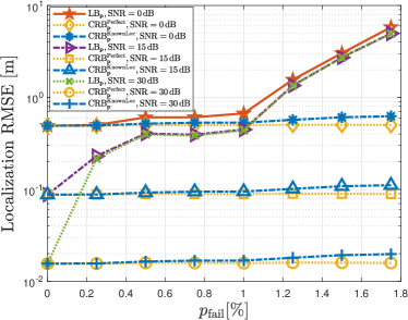
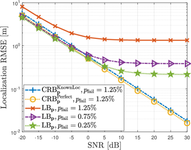
Figure 2: Theoretical limits on localization RMSE in (22), (24) and (27) versus 2 $p_{{\rm{fail}}}$ for various SNR values, and 2 SNR for various $p_{{\rm{fail}}}$ values. As ${\rm{CRB}}^{{\rm{Perfect}}}_{\bm{p}}$ and ${\rm{CRB}}^{{\rm{KnownLoc}}}_{\bm{p}}$ change only marginally with respect to $p_{{\rm{fail}}}$, they are plotted for a single value of $p_{{\rm{fail}}}$ in 2 to declutter the figure.

In Fig. 2, we report the theoretical limits on UE location estimation, derived in (22), (24) and (27), as a function of $p_{{\rm{fail}}}$ and ${\rm{SNR}}$. While obtaining the figures, the locations of faulty RIS elements for any given $p_{{\rm{fail}}}$ are fixed at random. For instance, if $p_{{\rm{fail}}}=2\%$, we randomly assign $Np_{{\rm{fail}}}=8$ failure locations and fix them. Then, we obtain the corresponding curves by averaging over $100$ distinct failure profiles (i.e., by considering $100$ distinct realizations of $(\kappa_{n},\psi_{n})$ pairs in (6) for the fixed failure locations).

We observe that ${\rm{CRB}}^{{\rm{Perfect}}}_{\bm{p}}$ and ${\rm{CRB}}^{{\rm{KnownLoc}}}_{\bm{p}}$ exhibit very similar values in the considered SNR and $p_{{\rm{fail}}}$ regimes. This suggests that once the locations of the failing RIS elements are known, knowing the respective failure coefficients $\zeta_{n}=\kappa_{n}e^{j\psi_{n}}$ brings only a marginal improvement in localization performance. Hence, the main bottleneck in RIS diagnosis with a UE having an a-priori unknown location lies in detection of the status (failing/functioning) of $N$ RIS elements from $T\ll N$ scalar observations, rather than estimation of their failure coefficients. In addition, we see that the gap between the LB and CRB curves becomes larger with increasing $p_{{\rm{fail}}}$ (i.e., as the mismatch between the true model in (III-A1) and the assumed model in (13) increases), as expected. When the UE is unaware of pixel failures, severe performance degradations can occur, especially at high SNRs (e.g., more than two orders-of-magnitude accuracy loss at ${\rm{SNR}}=30\,\rm{dB}$ for $p_{{\rm{fail}}}>1\%$). Therefore, even with small percentage of failures, employing failure-agnostic algorithms might lead to significant penalties in localization. Moreover, looking at the LB curves in Fig. 2, we observe that the localization performance saturates above a certain SNR level, reaching an SNR-independent bias value quantified by the second term in (21). This results from the mismatch between the true and assumed models, i.e., the price paid due to failures being ignored. Overall, we can conclude that RIS pixel failures can significantly degrade the localization performance, which necessitates the design of effective algorithms to mitigate their impact.

The high sensitivity of localization to pixel failures can be attributed to the fact that in the considered narrowband SISO setup with LoS blockage, information on UE location $\bm{p}$ derives only from the phase shifts across the RIS elements, as seen from the NF steering vector $\bm{a}(\bm{p})$ in (3) and the associated observations in (2). As pixel failures distort the phase profiles as specified in (5), the information that can be extracted from a set of scalar observations at the UE becomes quite inaccurate.

VI-C Performance of Algorithm 1 and Algorithm 2

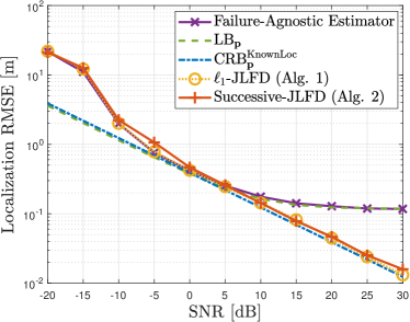
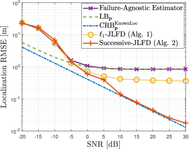
Figure 3: Localization RMSEs obtained by the failure-agnostic MS-unbiased estimator $\widehat{\bm{\eta}}(\bm{y})$ in (20) and the proposed algorithms, along with the theoretical bounds in (22) and (27), with respect to SNR for 3 $p_{{\rm{fail}}}=0.5\%$, and 3 $p_{{\rm{fail}}}=1\%$.

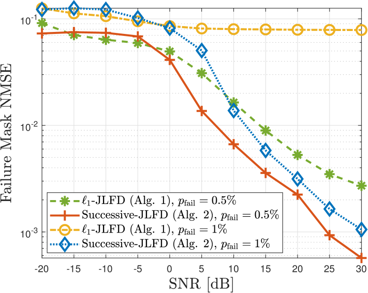
Figure 4: Mask recovery performances (mask NMSE in (52)) of Algorithm 1 and Algorithm 2 versus SNR for $p_{{\rm{fail}}}=0.5\%$ and $p_{{\rm{fail}}}=1\%$.

In this part, we examine the localization RMSE and mask recovery performances of Algorithm 1 and Algorithm 2. In Monte Carlo simulations, for a given $p_{{\rm{fail}}}$ value, $\lfloor Np_{{\rm{fail}}}\rfloor$ pixels out of $N$ are randomly chosen as failing and the corresponding failure coefficients represented by $(\kappa_{n},\psi_{n})$ are randomly generated. Given this single realization of the failure mask $\bm{m}$, the algorithm performances are evaluated by averaging over $100$ distinct noise realizations. In addition, the mask recovery performance is characterized through the normalized mean-squared-error (NMSE), defined as

$${\rm{NMSE}}=\frac{\left\lVert\widehat{\bm{m}}-\bm{m}\right\rVert^{2}_{2}}{\left\lVert\bm{m}\right\rVert^{2}_{2}}\leavevmode\nobreak\ ,$$ (52)

where $\widehat{\bm{m}}$ denotes the mask estimate.

In Fig. 3, we show the localization RMSEs achieved by the MS-unbiased estimator in (20) (i.e., the failure-agnostic benchmark), Algorithm 1 and Algorithm 2 as a function of SNR, along with the theoretical bounds, for $p_{{\rm{fail}}}=0.5\%$ and $p_{{\rm{fail}}}=1\%$. The corresponding mask NMSE performances of Algorithm 1 and Algorithm 2 are illustrated in Fig. 4. First, we see that the failure-agnostic MS-unbiased estimator in (20) achieves the corresponding LB asymptotically at high SNRs, which corroborates the MCRB analysis in Sec. III-A. In addition, it is observed that Algorithm 2 significantly outperforms the failure-agnostic estimator and attains the corresponding CRB at an SNR of $0$ and $10\leavevmode\nobreak\ \rm{dB}$ for $p_{{\rm{fail}}}=0.5\%$ and $p_{{\rm{fail}}}=1\%$, respectively, which demonstrates the effectiveness of the proposed successive JLFD strategy in recovering failure-induced performance degradations. Hence, Algorithm 2 can successfully yield accurate estimates of UE location in the presence of pixel failures and provide performance achievable under perfect knowledge of the failure mask $\bm{m}$ in (5), corresponding to a perfectly calibrated RIS. Moreover, by comparing Fig. 3 and Fig. 3, it appears that Algorithm 1 exhibits performance similar to that of Algorithm 2 for $p_{{\rm{fail}}}=0.5\%$, while it fails to achieve the theoretical limit for $p_{{\rm{fail}}}=1\%$ and reaches plateau in localization accuracy above a certain SNR level. This results from limited usage of the failure statistics in the $\ell_{1}$-regularization approach, in contrast with full exploitation of the statistics in the successive-JLFD approach. It is worth noting that the advantage of the $\ell_{1}$-regularization strategy lies in its low computational complexity, as investigated in Sec. V. Finally, the mask NMSE performances in Fig. 4 confirm the localization RMSE results in Fig. 3. Namely, Algorithm 1 cannot satisfactorily recover the failure mask for $p_{{\rm{fail}}}=1\%$, leading to gaps between the RMSE and the CRB in Fig. 3, while the mask NMSE of Algorithm 2 decreases consistently with SNR for both $p_{{\rm{fail}}}$ values.

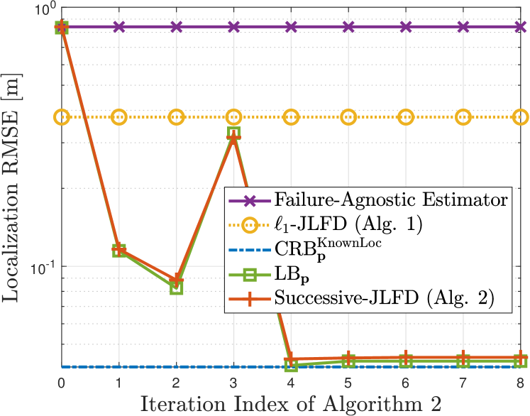
Figure 5: Evolution of localization RMSEs obtained by Algorithm 2 over successive iterations, along with the theoretical bounds in (22) and (27), the RMSEs of Algorithm 1 and the failure-agnostic estimator $\widehat{\bm{\eta}}(\bm{y})$ in (20), for SNR = $20\,\rm{dB}$ and $p_{{\rm{fail}}}=1\%$. At each iteration, which corresponds to detection of a single failure by Algorithm 2, ${\rm{LB}}_{\bm{p}}$ in (22) is computed by selecting the assumed model in (14) such that the UE assumes the presence of pixel failures detected up to and including the current iteration.

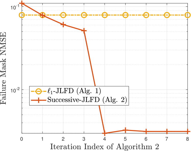
Figure 6: Evolution of mask recovery performances (mask NMSE in (52)) of Algorithm 2 over successive iterations, along with the mask NMSE of Algorithm 1, for SNR = $20\,\rm{dB}$ and $p_{{\rm{fail}}}=1\%$.

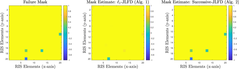
Figure 7: Illustration of failure mask $\bm{m}$ in (6) over the 2-D RIS plane, together with the mask estimates $\widehat{\bm{m}}$ obtained by Algorithm 1 and Algorithm 2, for SNR = $20\,\rm{dB}$ and $p_{{\rm{fail}}}=1\%$ (the real parts of the masks are presented).

To investigate the convergence behavior of Algorithm 2, we plot in Fig. 5 and Fig. 6 the evolution of localization and mask recovery performances of Algorithm 2 over successive iterations for SNR = $20\,\rm{dB}$ and $p_{{\rm{fail}}}=1\%$, together with ${\rm{CRB}}^{{\rm{KnownLoc}}}_{\bm{p}}$, ${\rm{LB}}_{\bm{p}}$ and the localization RMSEs of the failure-agnostic benchmark and Algorithm 1. It can be seen from Fig. 5 that starting from the location estimate of the failure-agnostic estimator, the proposed successive-JLFD algorithm can converge to the CRB by detecting pixel failures one-by-one at each iteration, leading to a successful progressive calibration procedure. We also emphasize that the RMSE of the successive-JLFD algorithm attains the corresponding LB at each iteration, which indicates the optimality of the proposed successive detection approach. In addition, it should not be surprising that the LB converges to the CRB as more failures are detected due to decreasing mismatch between the true and assumed models in (12) and (14), respectively. Moreover, we note that after the ${4^{\rm{th}}}$ iteration (corresponding to detection of $Np_{{\rm{fail}}}=4$ pixels), Algorithm 2 terminates and does not declare any new pixel as failing, and its performance coincides with the theoretical bound. This can also be observed from Fig. 6, where the mask NMSE of Algorithm 2 reaches its minimum at the ${4^{\rm{th}}}$ iteration. Overall, the results reveal the capability of Algorithm 2 to carry out UE localization and RIS diagnosis simultaneously, for the challenging SISO scenario under consideration.

Finally, to provide an illustrative example of failure mask recovery, Fig. 7 depicts the true failure mask and the instances of the estimated ones from Algorithm 1 and Algorithm 2 for SNR = $20\,\rm{dB}$ and $p_{{\rm{fail}}}=1\%$. We observe that Algorithm 2 performs significantly better than Algorithm 1 in detecting the pixel failures, and its coefficient estimates are very close to the true failure mask, in compliance with the aforementioned results and discussions.

VII Concluding Remarks

In this paper, we have addressed the problem of RIS-aided localization under pixel failures and investigated the impact of such failures on localization accuracy by conducting a comparative analysis of MCRB-based theoretical limits and standard CRB. To counteract the effect of failures, we have proposed two algorithms, namely $\ell_{1}$-JLFD and Successive-JLFD, for joint localization and mask recovery. Simulation results have offered valuable insights into the sensitivity of localization to pixel failures. In particular, we have observed that accuracy degradation caused by pixel failures can be significant (reaching as high as two orders-of-magnitude loss at high SNRs) even in the presence of small percentage of failing elements. This can be explained by noting that localization in the considered NF setup with LoS blockage relies completely on phase shifts across the RIS elements and even small number of failures can severely distort the received signal at the UE, preventing accurate location estimation. Remarkably, the proposed algorithms can drastically reduce the localization errors compared to the failure-agnostic estimator, and asymptotically attain the corresponding theoretical limits as the SNR increases, especially for Successive-JLFD. Potential future work includes investigation of the effect of spatial distribution of failures on localization accuracy and related mitigation strategies.

Appendix A PDF of Failure Coefficients

Let us define the random variable $\zeta=\kappa e^{j\psi}$, where $\kappa\sim\mathcal{U}(0,1)$ and $\psi\sim\mathcal{U}(-\pi,\pi)$ are independent random variables, by dropping the RIS element index $n$. There is a one-to-one mapping between $(\kappa,\psi)$ and $(\zeta_{\rm{R}},\zeta_{\rm{I}})$, where $\zeta_{\rm{R}}=\Re\left\{\zeta\right\}=\kappa\cos(\psi)$ and $\zeta_{\rm{I}}=\Im\left\{\zeta\right\}=\kappa\sin(\psi)$. Hence, for given $\zeta_{\rm{R}},\zeta_{\rm{I}}$, we can determine $\kappa,\psi$ as follows:

$$\kappa =\sqrt{\zeta_{\rm{R}}^{2}+\zeta_{\rm{I}}^{2}},$$ (53)

$$\psi =\begin{cases}\tan^{-1}\left(\frac{\zeta_{\rm{I}}}{\zeta_{\rm{R}}}\right),&\text{if }\zeta_{\rm{R}}\geq 0,\\ \tan^{-1}\left(\frac{\zeta_{\rm{I}}}{\zeta_{\rm{R}}}\right)-\pi,&\text{if }\zeta_{\rm{R}}<0,\zeta_{\rm{I}}<0,\\ \tan^{-1}\left(\frac{\zeta_{\rm{I}}}{\zeta_{\rm{R}}}\right)+\pi,&\text{if }\zeta_{\rm{R}}<0,\zeta_{\rm{I}}\geq 0.\end{cases}$$ (54)

Then, the Jacobian matrix can be calculated as

$$\mathbf{J}=\begin{bmatrix}\frac{\zeta_{\rm{R}}}{\sqrt{\zeta_{\rm{R}}^{2}+\zeta_{\rm{I}}^{2}}}&\frac{\zeta_{\rm{I}}}{\sqrt{\zeta_{\rm{R}}^{2}+\zeta_{\rm{I}}^{2}}}\\ \frac{-\zeta_{\rm{I}}}{{\zeta_{\rm{R}}^{2}+\zeta_{\rm{I}}^{2}}}&\frac{\zeta_{\rm{R}}}{{\zeta_{\rm{R}}^{2}+\zeta_{\rm{I}}^{2}}}\end{bmatrix}\leavevmode\nobreak\ .$$ (55)

This implies

$$f_{\zeta}(\zeta_{\rm{R}},\zeta_{\rm{I}})=f_{\kappa}(\kappa)f_{\psi}(\psi)\lvert\mathbf{J}\rvert=\frac{1}{2\pi\sqrt{\zeta_{\rm{R}}^{2}+\zeta_{\rm{I}}^{2}}}$$ (56)

for $\zeta_{\rm{R}}^{2}+\zeta_{\rm{I}}^{2}\leq 1$. In a more compact form,

$$f_{\zeta}(\zeta)=\begin{cases}\frac{1}{2\pi\lvert\zeta\rvert},&\leavevmode\nobreak\ \leavevmode\nobreak\ \lvert\zeta\rvert\leq 1\\ 0,&\leavevmode\nobreak\ \leavevmode\nobreak\ \textrm{otherwise}\end{cases}\leavevmode\nobreak\ .$$ (57)

Appendix B Computation of (47)

The second term in (47) can be obtained from (8) and (46) as follows:

$$\sum_{n=1}^{N}\log f_{m_{n}}([\widetilde{\bm{m}}_{k}]_{n})=(N-1-\lvert\mathcal{I}^{(i-1)}\rvert)\log(1-p_{{\rm{fail}}})$$

$$\leavevmode\nobreak\ \leavevmode\nobreak\ +(\lvert\mathcal{I}^{(i-1)}\rvert+1)\log p_{{\rm{fail}}}+\sum_{n\in\mathcal{I}^{(i-1)}}\log f_{\zeta_{n}}([\bm{m}^{(i-1)}]_{n})$$

$$\leavevmode\nobreak\ \leavevmode\nobreak\ +\log f_{\zeta_{k}}(\zeta_{k})$$ (58)

for $k\geq 1$, and

$$\sum_{n=1}^{N}\log f_{m_{n}}([\widetilde{\bm{m}}_{k}]_{n})=(N-\lvert\mathcal{I}^{(i-1)}\rvert)\log(1-p_{{\rm{fail}}})$$ (59)

$$+\lvert\mathcal{I}^{(i-1)}\rvert\log p_{{\rm{fail}}}+\sum_{n\in\mathcal{I}^{(i-1)}}\log f_{\zeta_{n}}([\bm{m}^{(i-1)}]_{n})$$

for $k=0$.

References

• [1] Q. Wu et al., “Intelligent reflecting surface-aided wireless communications: A tutorial,” IEEE Transactions on Communications, vol. 69, no. 5, pp. 3313–3351, 2021.
• [2] Z. Chen et al., “Intelligent reflecting surface assisted terahertz communications toward 6G,” IEEE Wireless Communications, vol. 28, no. 6, pp. 110–117, 2021.
• [3] C. Pan et al., “Reconfigurable Intelligent Surfaces for 6G Systems: Principles, Applications, and Research Directions,” IEEE Communications Magazine, vol. 59, no. 6, pp. 14–20, 2021.
• [4] C. Huang et al., “Reconfigurable intelligent surfaces for energy efficiency in wireless communication,” IEEE Transactions on Wireless Communications, vol. 18, no. 8, pp. 4157–4170, 2019.
• [5] Z. Yang et al., “Energy-efficient wireless communications with distributed reconfigurable intelligent surfaces,” IEEE Transactions on Wireless Communications, vol. 21, no. 1, pp. 665–679, 2022.
• [6] C. Huang et al., “Reconfigurable intelligent surface assisted multiuser MISO systems exploiting deep reinforcement learning,” IEEE Journal on Selected Areas in Communications, vol. 38, no. 8, pp. 1839–1850, 2020.
• [7] H. Guo et al., “Weighted sum-rate maximization for reconfigurable intelligent surface aided wireless networks,” IEEE Transactions on Wireless Communications, vol. 19, no. 5, pp. 3064–3076, 2020.
• [8] W. Wang et al., “Joint beam training and positioning for intelligent reflecting surfaces assisted millimeter wave communications,” IEEE Transactions on Wireless Communications, vol. 20, no. 10, pp. 6282–6297, 2021.
• [9] A. Elzanaty et al., “Reconfigurable intelligent surfaces for localization: Position and orientation error bounds,” IEEE Trans. Signal Process., vol. 69, pp. 5386–5402, 2021.
• [10] H. Wymeersch et al., “Radio localization and mapping with reconfigurable intelligent surfaces: Challenges, opportunities, and research directions,” IEEE Vehicular Technology Magazine, vol. 15, no. 4, pp. 52–61, 2020.
• [11] E. Björnson et al., “Reconfigurable intelligent surfaces: A signal processing perspective with wireless applications,” IEEE Signal Processing Magazine, vol. 39, no. 2, pp. 135–158, 2022.
• [12] D. Dardari et al., “LOS/NLOS near-field localization with a large reconfigurable intelligent surface,” IEEE Transactions on Wireless Communications, vol. 21, no. 6, pp. 4282–4294, 2022.
• [13] O. Rinchi et al., “Compressive near-field localization for multipath RIS-aided environments,” IEEE Communications Letters, vol. 26, no. 6, pp. 1268–1272, 2022.
• [14] C. Ozturk et al., “RIS-aided near-field localization under phase-dependent amplitude variations,” IEEE Transactions on Wireless Communications, accepted for publication, 2023.
• [15] Z. Abu-Shaban et al., “Near-field localization with a reconfigurable intelligent surface acting as lens,” in ICC 2021 - IEEE International Conference on Communications, 2021, pp. 1–6.
• [16] C. Öztürk et al., “On the impact of hardware impairments on RIS-aided localization,” in ICC 2022 - IEEE International Conference on Communications, 2022, pp. 2846–2851.
• [17] M. Rahal et al., “Constrained RIS phase profile optimization and time sharing for near-field localization,” in 2022 IEEE 95th Vehicular Technology Conference: (VTC2022-Spring), 2022, pp. 1–6.
• [18] M. Luan et al., “Phase design and near-field target localization for RIS-assisted regional localization system,” IEEE Transactions on Vehicular Technology, vol. 71, no. 2, pp. 1766–1777, 2022.
• [19] X. Zhang et al., “Hybrid reconfigurable intelligent surfaces-assisted near-field localization,” IEEE Communications Letters, pp. 1–1, 2022.
• [20] M. E. Eltayeb et al., “Compressive sensing for millimeter wave antenna array diagnosis,” IEEE Transactions on Communications, vol. 66, no. 6, pp. 2708–2721, 2018.
• [21] B. Sun et al., “Direction-of-arrival estimation under array sensor failures with ULA,” IEEE Access, vol. 8, pp. 26 445–26 456, 2020.
• [22] H. Taghvaee et al., “Error analysis of programmable metasurfaces for beam steering,” IEEE Journal on Emerging and Selected Topics in Circuits and Systems, vol. 10, no. 1, pp. 62–74, 2020.
• [23] R. Sun et al., “Diagnosis of intelligent reflecting surface in millimeter-wave communication systems,” IEEE Transactions on Wireless Communications, vol. 21, no. 6, pp. 3921–3934, 2022.
• [24] J. Zhang et al., “Phase calibration for intelligent reflecting surfaces assisted millimeter wave communications,” IEEE Transactions on Signal Processing, vol. 70, pp. 1026–1040, 2022.
• [25] K. Wang et al., “Doppler effect mitigation using reconfigurable intelligent surfaces with hardware impairments,” in 2021 IEEE Globecom Workshops (GC Wkshps), 2021, pp. 1–6.
• [26] S. Ma et al., “Joint diagnosis of RIS and BS for RIS-aided millimeter-wave system,” Electronics, vol. 10, no. 20, 2021. [Online]. Available: https://www.mdpi.com/2079-9292/10/20/2556
• [27] B. Li et al., “Joint array diagnosis and channel estimation for RIS-aided mmwave MIMO system,” IEEE Access, vol. 8, pp. 193 992–194 006, 2020.
• [28] S. Fortunati et al., “Performance bounds for parameter estimation under misspecified models: Fundamental findings and applications,” IEEE Signal Processing Magazine, vol. 34, no. 6, pp. 142–157, 2017.
• [29] J. Lee et al., “Channel estimation via orthogonal matching pursuit for hybrid MIMO systems in millimeter wave communications,” IEEE Transactions on Communications, vol. 64, no. 6, pp. 2370–2386, 2016.
• [30] A. Shahmansoori et al., “Position and orientation estimation through millimeter-wave MIMO in 5G systems,” IEEE Transactions on Wireless Communications, vol. 17, no. 3, pp. 1822–1835, 2018.
• [31] E. Grossi et al., “Adaptive detection and localization exploiting the IEEE 802.11ad standard,” IEEE Transactions on Wireless Communications, vol. 19, no. 7, pp. 4394–4407, 2020.
• [32] J.-W. Tao et al., “Joint DOA, range, and polarization estimation in the Fresnel region,” IEEE Transactions on Aerospace and Electronic Systems, vol. 47, no. 4, pp. 2657–2672, 2011.
• [33] V. R. Gowda et al., “Wireless power transfer in the radiative near field,” IEEE Antennas and Wireless Propagation Letters, vol. 15, pp. 1865–1868, 2016.
• [34] A. Guerra et al., “Near-field tracking with large antenna arrays: Fundamental limits and practical algorithms,” IEEE Transactions on Signal Processing, vol. 69, pp. 5723–5738, 2021.
• [35] K. Keykhosravi et al., “RIS-enabled SISO localization under user mobility and spatial-wideband effects,” IEEE Journal of Selected Topics in Signal Processing, pp. 1–1, 2022.
• [36] F. Guidi et al., “Radio positioning with EM processing of the spherical wavefront,” IEEE Transactions on Wireless Communications, vol. 20, no. 6, pp. 3571–3586, 2021.
• [37] J. Ziniel et al., “Dynamic compressive sensing of time-varying signals via approximate message passing,” IEEE Transactions on Signal Processing, vol. 61, no. 21, pp. 5270–5284, 2013.
• [38] A.-S. Sheikh et al., “A truncated EM approach for spike-and-slab sparse coding,” Journal of Machine Learning Research, vol. 15, no. 1, pp. 2653–2687, 2014.
• [39] I. J. Goodfellow et al., “Scaling up spike-and-slab models for unsupervised feature learning,” IEEE Transactions on Pattern Analysis and Machine Intelligence, vol. 35, no. 8, pp. 1902–1914, 2013.
• [40] S. Fortunati et al., “Chapter 4: Parameter bounds under misspecified models for adaptive radar detection,” in Academic Press Library in Signal Processing, Volume 7, R. Chellappa et al., Eds.   Academic Press, 2018, pp. 197–252.
• [41] S. M. Kay, Fundamentals of statistical signal processing: estimation theory.   Prentice-Hall, Inc., 1993.
• [42] Y. Noam et al., “Notes on the tightness of the hybrid Cramér–Rao lower bound,” IEEE Transactions on Signal Processing, vol. 57, no. 6, pp. 2074–2084, 2009.
• [43] L. A. Wolsey, “Mixed integer programming,” Wiley Encyclopedia of Computer Science and Engineering, pp. 1–10, 2007.
• [44] R. J. Tibshirani, “The LASSO problem and uniqueness,” Electronic Journal of statistics, vol. 7, pp. 1456–1490, 2013.
• [45] M. Grant et al., “CVX: Matlab software for disciplined convex programming, version 2.1,” http://cvxr.com/cvx, Mar. 2014.
• [46] A. Beck et al., “A fast iterative shrinkage-thresholding algorithm for linear inverse problems,” SIAM Journal on Imaging Sciences, vol. 2, no. 1, pp. 183–202, Mar. 2009.
• [47] S. Mallat et al., “Matching pursuits with time-frequency dictionaries,” IEEE Transactions on Signal Processing, vol. 41, no. 12, pp. 3397–3415, 1993.
• [48] A. Beck et al., “A fast iterative shrinkage-thresholding algorithm for linear inverse problems,” SIAM Journal on Imaging Sciences, vol. 2, no. 1, pp. 183–202, 2009. [Online]. Available: https://doi.org/10.1137/080716542
• [49] C. Baquero Barneto et al., “Millimeter-wave mobile sensing and environment mapping: Models, algorithms and validation,” IEEE Transactions on Vehicular Technology, vol. 71, no. 4, pp. 3900–3916, 2022.