Efficient numerical methods for the Navier-Stokes-Nernst-Planck-Poisson equations^∗

Abstract.

We propose in this paper efficient first/second-order time-stepping schemes for the evolutional Navier-Stokes-Nernst-Planck-Poisson equations. The proposed schemes are constructed using an auxiliary variable reformulation and sophisticated treatment of the terms coupling different equations. By introducing a dynamic equation for the auxiliary variable and reformulating the original equations into an equivalent system, we construct first- and second-order semi-implicit linearized schemes for the underlying problem. The main advantages of the proposed method are: (1) the schemes are unconditionally stable in the sense that a discrete energy keeps decay during the time stepping; (2) the concentration components of the discrete solution preserve positivity and mass conservation; (3) the delicate implementation shows that the proposed schemes can be very efficiently realized, with computational complexity close to a semi-implicit scheme. Some numerical examples are presented to demonstrate the accuracy and performance of the proposed method. As far as the best we know, this is the first second-order method which satisfies all the above properties for the Navier-Stokes-Nernst-Planck-Poisson equations.

1. Introduction and motivation

The Navier-Stokes-Nernst-Planck-Poisson (NSNPP) coupling system is a popular model for describing the electro-hydrodynamic phenomenon, which is originated in bio-electronic application. It is also known as the electro-fluid-dynamics, used to study the dynamics of electrically charged fluids, the motions of ionized particles or molecules and their interactions with electric fields and the surrounding fluid. In electro fluid dynamics, ions of different valences suspended in a fluid are carried by the fluid flow and an electric potential, which results from both an applied potential on the boundary and the distribution of charges carried by the ions. In addition, ionic diffusion is driven by the concentration gradients of the ions themselves. In turn, fluid flow is forced by the electrical field created by the ions. These situations arise frequently in a large number of physical, biophysical, and industrial processes. For more details of the physical background issues of this system, we refer the reader to [24, 2] and the references therein.

The mathematical property of the NSNPP system has been investigated in a number of papers. Local existence of solutions in the whole space was obtained in [14]. Schmuck in [26] established global existence and uniqueness of weak solutions in a bounded domain in two and three dimensions for blocking boundary conditions on the ions and homogeneous Neumann boundary condition on the potential. Ryham [25] considered the homogeneous Dirichlet boundary conditions on the potential, and gave the global existence of weak solutions in two dimensions for large initial data and in three dimensions for small initial data and forces. Bothe [3] studied the Robin boundary conditions for the electric potential, and showed the global existence and stability in two dimensions. Zhao et al. [35] proved the local well-posedness for any initial data and global well-posedness for small initial data in the critical Lebesgue spaces. Deng et al. [9] extended this result to Triebel-Lizorkin space and Besov space with negative indices. Zhang [34] proved the global existence for the Cauchy problem in two dimensions and established the $L^{2}$ decay estimates of solutions by using the Fourier splitting method. Constantin [7, 8, 22] investigated the global existence of smooth solutions for different boundary conditions.

Numerical methods for the NSNPP system have also been subject of several works. Yang et al. [32] proposed an artificial compressibility method and a finite difference/alternative direction method. Tsai et al. [31] employed this method in capillary electrophoresis microchips, and tested some injection systems with different configurations. Prohl and Schmuck [23] used finite element method for spatial discretization and an implicit time discretization which preserves the non-negativity of the ionic concentrations. They also considered a projection method without non-negativity preserving. He and Sun [11] proposed some time stepping and finite element methods for NSNPP, which preserves the positivity and/or some form of energy dissipation under certain conditions and specific spatial discretization. The drawback of these methods is the need to solve nonlinear equations at each time step. Liu and Xu [20] proposed numerical methods of different orders by combining several finite difference schemes in time and a spectral method for the spatial discretization. The proposed schemes result in several elliptic equations with time-dependent coefficient to be solved at every time step. The positivity-preserving of the first-order scheme was proved.

The scalar auxiliary variable approach, often called SAV [28, 29], has received much attention recently. It has been proved to be a powerful tool to design unconditionally stable schemes for a large class of problems [5, 6, 12, 36, 19, 18, 16, 33, 15]. The aim of this paper is to make use of the auxiliary variable approach to construct highly efficient time-stepping schemes for the NSNPP equations. Precisely, our idea is to find a suitable auxiliary variable to treat the nonlinear terms involved in the equations, and employ a splitting strategy to decouple different unknowns in the Navier-Stokes part. A function transform approach for Nernst-Plank-Poisson will be also employed in the construction. We will show that the resulting scheme possesses the following properties:

- it is positivity preserving;

- it is mass conservative;

- it is unconditionally energy dissipative;

- it can be implemented in an efficient way: the computational complexity is equal to solving several decoupled linear equations with constant coefficient at each time step.

The spatial discretization will make use of a spectral-Galerkin method in [27], for which fast solvers exist for elliptic equations with constant coefficients. We emphasize that the above attractive properties remain held at the full discrete level.

The remainder of this paper is structured as follows. In Section 2, we first describe the NSNPP system, and the reformulation based on auxiliary variable approach. In Section 3, we construct and analyze first/second order, linear, decoupled, and unconditionally stable scheme for the reformulate NSNPP equations. We describe in Section 4 the implementation details of the proposed schemes, and show that the schemes can be efficiently implemented through solving a set of decoupled, linear elliptic equations with constant coefficients. In Section 5, we present numerical examples to validate our schemes. Some concluding remarks are given in Section 6.

2. Governing equations and reformulatation

2.1. Navier-Stokes-Nernst-Planck-Poisson equations

Let $\Omega\in{\mathbb{R}}^{2}$ be a bounded Lipschitz domain and $T>0$. Given initial conditions $\mathbf{u}({\boldsymbol{x}},0),c_{i}({\boldsymbol{x}},0)$ $(i=1,...,m)$. We look for the velocity field $\mathbf{u}({\boldsymbol{x}},t)$, the pressure $p({\boldsymbol{x}},t)$, the mass concentration of ions $c_{i}({\boldsymbol{x}},t)$ $(i=1,...,m)$, and the electrostatic potential $\Phi({\boldsymbol{x}},t)$, satisfying the following Navier-Stokes-Nernst-Plank-Poisson equations (NSNPP) in $\Omega\times(0,T]$:

$$\partial_{t}\mathbf{u}+(\mathbf{u}\cdot\nabla)\mathbf{u}-\nu\Delta\mathbf{u}+\nabla p=-\big{(}\sum_{i=1}^{m}z_{i}c_{i}\big{)}\nabla\Phi,$$ (2.1a)

$$\nabla\cdot\mathbf{u}=0,$$ (2.1b)

$$\partial_{t}c_{i}=D_{i}\nabla\cdot\left(\nabla c_{i}+z_{i}c_{i}\nabla\Phi\right)-\nabla\cdot(\mathbf{u}c_{i}),\quad i=1,...,m,$$ (2.1c)

$$-\epsilon\Delta\Phi=\sum_{i=1}^{m}z_{i}c_{i},$$ (2.1d)

where $z_{i}\in{\mathbb{R}}$ are the ionic valences, $D_{i}$ denote the positive constant diffusivities, $\epsilon>0$ is a small positive dimensionless number representing the ratio of the squared Debye length to the physical characteristic length, $\nu>0$ is the kinematic viscosity.

We consider the blocking boundary conditions, i.e., vanishing of all normal fluxes for the ionic concentrations:

$$\big{(}\mathbf{u}c_{i}-D_{i}(\nabla c_{i}+z_{i}c_{i}\nabla\Phi)\big{)}\cdot\mathbf{n}\big{|}_{\partial\Omega}=0,\ i=1,...,m,$$ (2.2)

where $\mathbf{n}$ is outer normal on the boundary of $\partial\Omega$. The boundary condition on the velocity $\mathbf{u}$ and the potential $\Phi$ is respectively

$$\mathbf{u}\big{|}_{\partial\Omega}=0,$$ (2.3)

and

$$\frac{\partial\Phi}{\partial\mathbf{n}}\Big{|}_{\partial\Omega}=0.$$ (2.4)

Under the conditions (2.3) and (2.4), noticing the identity $\nabla c=c\nabla\log c$, it follows from (2.2):

$$c_{i}\frac{\partial(\log c_{i}+z_{i}\Phi)}{\partial\mathbf{n}}\Big{|}_{\partial\Omega}=(\frac{\partial c_{i}}{\partial\mathbf{n}}+z_{i}c_{i}\frac{\partial\Phi}{\partial\mathbf{n}})\Big{|}_{\partial\Omega}=\frac{\partial c_{i}}{\partial\mathbf{n}}\Big{|}_{\partial\Omega}=0,\ i=1,...,m.$$ (2.5)

It is readily seen that in the governing equations (2.1a)-(2.1d), the pressure $p$ and electrostatic potential $\Phi$ are determined up to an arbitrary constant. In order to fix this constant, we impose the following zero mean conditions:

$$\int_{\Omega}pd{\boldsymbol{x}}=0,\quad\int_{\Omega}\Phi d{\boldsymbol{x}}=0.$$ (2.6)

We define two partial energy functionals $E_{ns},E_{npp}$:

$$E_{ns}=E_{ns}[\mathbf{u}]:=\frac{1}{2}\int_{\Omega}|\mathbf{u}|^{2}d{\boldsymbol{x}},$$

$$E_{npp}=E_{npp}[\{c_{i}\},\Phi]:=\int_{\Omega}\Big{[}\sum_{i=1}^{m}c_{i}(\log c_{i}-1)+\frac{1}{2}\big{(}\sum_{i=1}^{m}z_{i}c_{i}\big{)}\Phi\Big{]}d{\boldsymbol{x}}.$$

The total energy functional is defined as the sum of these two partial functionals:

$$E={E}[\mathbf{u},\{c_{i}\},\Phi]:=E_{ns}+E_{npp}.$$ (2.8)

Using $\nabla\cdot\mathbf{u}=0$ and the boundary conditions (2.3), (2.4), and (2.5), we have

$$\displaystyle\frac{dE_{ns}}{dt} =\int_{\Omega}\partial_{t}\mathbf{u}\cdot\mathbf{u}d{\boldsymbol{x}}=\int_{\Omega}\Big{[}-(\mathbf{u}\cdot\nabla)\mathbf{u}+\nu\Delta\mathbf{u}-\nabla p-\big{(}\sum_{i=1}^{m}z_{i}c_{i}\big{)}\nabla\Phi\Big{]}\cdot\mathbf{u}d{\boldsymbol{x}}$$

$$=-\nu\int_{\Omega}|\nabla\mathbf{u}|^{2}d{\boldsymbol{x}}-\int_{\Omega}\big{(}\sum_{i=1}^{m}z_{i}c_{i}\big{)}\nabla\Phi\cdot\mathbf{u}d{\boldsymbol{x}}.$$ (2.9)

Taking the inner product of (2.1c) with $\log c_{i}+z_{i}\Phi$, summing up for $i=1,...,m$, and using (2.1d), we obtain the following equality:

$$\displaystyle\frac{dE_{npp}}{dt} =\displaystyle\sum_{i=1}^{m}\int_{\Omega}-D_{i}c_{i}|\nabla(\log c_{i}+z_{i}\Phi)|^{2}d{\boldsymbol{x}}+\sum_{i=1}^{m}\int_{\Omega}-\nabla\cdot(\mathbf{u}c_{i})(\log c_{i}+z_{i}\Phi)d{\boldsymbol{x}}.$$ (2.10)

Furthermore, for the second term in the right hand side, we have

$$\displaystyle\sum_{i=1}^{m}\int_{\Omega}-\nabla\cdot(\mathbf{u}c_{i})(\log c_{i}+z_{i}\Phi)d{\boldsymbol{x}} =\sum_{i=1}^{m}\int_{\Omega}(\mathbf{u}c_{i})\cdot\nabla(\log c_{i}+z_{i}\Phi)d{\boldsymbol{x}}$$

$$=\sum_{i=1}^{m}\int_{\Omega}\mathbf{u}\cdot\nabla c_{i}d{\boldsymbol{x}}+\int_{\Omega}(\sum_{i=1}^{m}z_{i}c_{i})\mathbf{u}\cdot\nabla\Phi d{\boldsymbol{x}}=\int_{\Omega}(\sum_{i=1}^{m}z_{i}c_{i})\mathbf{u}\cdot\nabla\Phi d{\boldsymbol{x}}.$$ (2.11)

Then, combining (2.1), (2.10), and (2.1) gives

$$\displaystyle\frac{dE}{dt}= -\nu\int_{\Omega}|\nabla\mathbf{u}|^{2}d{\boldsymbol{x}}-\sum_{i=1}^{m}\int_{\Omega}D_{i}c_{i}|\nabla(\log c_{i}+z_{i}\Phi)|^{2}d{\boldsymbol{x}}.$$ (2.12)

Lemma 2.1.

The NSNPP problem (2.1)-(2.4) satisfies the following properties:

1) Mass conservation:

$$\int_{\Omega}c_{i}({\boldsymbol{x}},t)d{\boldsymbol{x}}=\int_{\Omega}c_{i}({\boldsymbol{x}},0)d{\boldsymbol{x}},\ \ \forall t>0.$$ (2.13)

2) Positivity: If the initial condition $c_{i}({\boldsymbol{x}},0)>0\ a.e.\ {\boldsymbol{x}}\in\Omega$, then $c_{i}({\boldsymbol{x}},t)>0\ a.e.\ {\boldsymbol{x}}\in\Omega,\ t\in[0,T]$.

3) Energy dissipation:

$$\frac{dE}{dt}\leq 0.$$ (2.14)

Proof.

The proof is simple, and can be found in the literature. We give a proof sketch here for the convenience of the reader.

1) Integrating (2.1c) over $\Omega$, and using (2.1b), we obtain immediately (2.13).

2) A proof of the positivity was given in [26].

3) (2.12) leads to the desired result (2.14). ∎

2.2. Auxiliary variable reformulation

Observing that $\int_{\Omega}\sum_{i=1}^{m}c_{i}(\log c_{i}-1)d{\boldsymbol{x}}$ is convex, so there is a constant $C_{0}>0$, such that $E_{npp}[\{c_{i}\},\Phi]+C_{0}\geq 1$. We introduce the time-dependent auxiliary variable (AV) as follows:

$$r(t):=\sqrt{E_{npp}[\{c_{i}\},\Phi]+C_{0}}.$$ (2.15)

Then we have

$$\frac{dr}{dt}=\displaystyle\frac{1}{2\sqrt{E_{npp}+C_{0}}}\frac{dE_{npp}}{dt}.$$

Insert (2.10) into the above equation, add the zero-valued item $\int_{\Omega}\mathbf{u}\cdot\nabla\mathbf{u}\cdot\mathbf{u}d{\boldsymbol{x}}$, and multiply by the factor $\frac{r(t)}{\sqrt{E_{npp}[\{c_{i}\},\Phi]+C_{0}}}$, the governing equation for the auxiliary variable $r(t)$ can be obtained as follows:

$$\displaystyle\frac{dr(t)}{dt}=\displaystyle-\frac{1}{2\sqrt{E_{npp}+C_{0}}}\bigg{[}\frac{r(t)}{\sqrt{E_{npp}[\{c_{i}\},\Phi]+C_{0}}}\sum_{i=1}^{m}\int_{\Omega}D_{i}c_{i}|\nabla\mu_{i}|^{2}d{\boldsymbol{x}}-$$

$$\int_{\Omega}\big{(}\sum_{i=1}^{m}z_{i}c_{i}\big{)}\nabla\Phi\cdot\mathbf{u}d{\boldsymbol{x}}-\int_{\Omega}(\mathbf{u}\cdot\nabla)\mathbf{u}\cdot\mathbf{u}d{\boldsymbol{x}}\bigg{]}.$$

For the Nernst-Plank-Poisson part, in order to preserve the positivity of the concentrations $c_{i}$, we consider the variable transformation technique, which has already been used in a number of papers; see [1, 21, 4, 13]:

$$c_{i}=T(\sigma_{i}):=\exp(\sigma_{i}),\quad i=1,...,m,$$ (2.16)

where $\{\sigma_{i}\}_{i=1}^{m}$ are the new unknown functions to be determined. Using this variable change, the boundary conditions (2.5) are switched to

$$\frac{\partial\sigma_{i}}{\partial\mathbf{n}}\Big{|}_{\partial\Omega}=0,\ i=1,...,m.$$ (2.17)

With the auxiliary variable $r$ and the additional unknown variables $\{\sigma_{i}\}_{i=1}^{m}$, we have the complete set of equations as follows:

$$\partial_{t}\mathbf{u}+\frac{r(t)}{\sqrt{E_{npp}(t)+C_{0}}}\Big{(}(\mathbf{u}\cdot\nabla)\mathbf{u}+\big{(}\sum_{i=1}^{m}z_{i}c_{i}\big{)}\nabla\Phi\Big{)}-\nu\Delta\mathbf{u}+\nabla p=0,$$ (2.18a)

$$\nabla\cdot\mathbf{u}=0,$$ (2.18b)

$$\partial_{t}\sigma_{i}=D_{i}\Delta\sigma_{i}+D_{i}\big{(}|\nabla\sigma_{i}|^{2}+z_{i}(\nabla\sigma_{i}\cdot\nabla\Phi+\Delta\Phi)\big{)}-\nabla\cdot(\sigma_{i}\mathbf{u}),$$ (2.18c)

$$c_{i}=\exp(\sigma_{i}),\quad i=1,...,m,$$ (2.18d)

$$-\epsilon\Delta\bar{\Phi}=\sum_{i=1}^{m}z_{i}c_{i},$$ (2.18e)

$$\frac{dr(t)}{dt}=-\displaystyle\frac{1}{2\sqrt{E_{npp}(t)+C_{0}}}\Big{[}\frac{r(t)}{\sqrt{E_{npp}(t)+C_{0}}}\sum_{i=1}^{m}\int_{\Omega}D_{i}c_{i}|\nabla(\log c_{i}+z_{i}\Phi)|^{2}d{\boldsymbol{x}}$$

$$\qquad\qquad-\int_{\Omega}\big{(}\sum_{i=1}^{m}z_{i}c_{i}\big{)}\nabla\Phi\cdot\mathbf{u}d{\boldsymbol{x}}-\int_{\Omega}(\mathbf{u}\cdot\nabla)\mathbf{u}\cdot\mathbf{u}d{\boldsymbol{x}}\Big{]},$$ (2.18f)

$$\Phi=\frac{r(t)}{\sqrt{E_{npp}(t)+C_{0}}}\bar{\Phi},$$ (2.18g)

subject to the boundary conditions (2.3), (2.4), (2.17), and the initial conditions:

$${\mathbf{u}}({\boldsymbol{x}},0)={\mathbf{u}}_{0}({\boldsymbol{x}}),$$ (2.19)

$$r(0)=\sqrt{E_{npp}[\{c_{i}({\boldsymbol{x}},0)\},\ \Phi({\boldsymbol{x}},0)]+C_{0}}.$$ (2.20)

Noticing that $\int_{\Omega}(\mathbf{u}\cdot\nabla)\mathbf{u}\cdot\mathbf{u}d{\boldsymbol{x}}\equiv 0$ and $\frac{r(t)}{\sqrt{E_{npp}(t)+C_{0}}}\equiv 1$, it is not difficult to check that the reformulated system (2.18) is strictly equivalent to the original system (2.1) at the continuous level.

Taking the $L^{2}$ inner products of equation (2.18a) with $\mathbf{u}$, equation (2.18f) with $2r$ respectively, then summing the resultants together, we obtain the following energy dissipation law:

$$\frac{d}{dt}\Big{(}\int_{\Omega}\frac{1}{2}|\mathbf{u}|^{2}d{\boldsymbol{x}}+r^{2}\Big{)}=-\nu\int_{\Omega}|\nabla\mathbf{u}|^{2}d{\boldsymbol{x}}-\Big{|}\frac{r(t)}{\sqrt{E_{npp}(t)+C_{0}}}\Big{|}^{2}\sum_{i=1}^{m}\int_{\Omega}D_{i}c_{i}|\nabla\mu_{i}|^{2}d{\boldsymbol{x}}\leq 0.$$

Next we focus on the equivalent system (2.18) and construct numerical methods for this system.

3. Unconditionally stable time-stepping schemes

Let $\Delta t$ be the time step size, $n\geq 0$ denotes the time step index, and $(\cdot)^{n}$ denotes the variable $(\cdot)$ at the time step $n$. Let

$$\mathbf{u}^{0}=\mathbf{u}({\boldsymbol{x}},0),\quad c_{i}^{0}=c_{i}({\boldsymbol{x}},0),\quad r^{0}=r(0).$$ (3.1)

$\Phi^{0}$ and $p^{0}$ are obtained by solving the equations (2.1d) and (2.1a) at $t=0$ under the constraint (2.6), which read respectively in their weak forms:

$$\epsilon\int_{\Omega}\nabla\Phi^{0}\cdot\nabla qd{\boldsymbol{x}}=\int_{\Omega}\big{(}\sum_{i=1}^{m}z_{i}c_{i}^{0}\big{)}qd{\boldsymbol{x}},\quad\forall q\in H^{1}(\Omega).$$ (3.2)

$$\int_{\Omega}\nabla p^{0}\cdot\nabla qd{\boldsymbol{x}}=\int_{\Omega}\Big{(}-\big{(}\sum_{i=1}^{m}z_{i}c_{i}^{0}\big{)}\nabla\Phi^{0}-\mathbf{u}^{0}\cdot\nabla\mathbf{u}^{0}\Big{)}\cdot\nabla qd{\boldsymbol{x}},\quad\forall q\in H^{1}(\Omega).$$ (3.3)

3.1. Time stepping schemes

We now propose different schemes using first/second order BDF for the equivalent system (2.18).

Scheme1: The first scheme is constructed by making use of BDF1 and some first order approximations to different terms in (2.18a)-(2.18g): given the initial data $(u^{0},p^{0},\Phi^{0},\{c_{i}^{0}\},r^{0})$, compute $(u^{n+1},p^{n+1},\Phi^{n+1},\{c_{i}^{n+1}\},r^{n+1})$ for $n\geq 0$ successively by solving

$$\frac{\sigma_{i}^{n+1}-\sigma_{i}^{n}}{\Delta t}-D_{i}\Delta\sigma_{i}^{n+1}=$$

$$\hskip 28.45274ptD_{i}\big{[}|\nabla\sigma_{i}^{n}|^{2}+z_{i}(\nabla\sigma_{i}^{n}\cdot\nabla\Phi^{n}+\Delta\Phi^{n})\big{]}-\nabla\cdot(\sigma_{i}^{n}\mathbf{u}^{n}),\text{ with }\left.\frac{\partial\sigma_{i}^{n+1}}{\partial\mathbf{n}}\right|_{\partial\Omega}=0,$$ (3.4a)

$$\bar{c}_{i}^{n+1}=\exp(\sigma_{i}^{n+1}),$$ (3.4b)

$$\lambda_{i}^{n+1}\int_{\Omega}\bar{c}_{i}^{n+1}-\int_{\Omega}c_{i}^{n}=0,$$ (3.4c)

$$c_{i}^{n+1}=\lambda_{i}^{n+1}\bar{c}_{i}^{n+1},\ \ i=1,...,m,$$ (3.4d)

$$-\epsilon\Delta\bar{\Phi}^{n+1}=\sum_{i=1}^{m}z_{i}c_{i}^{n+1},\quad\text{ with }\int_{\Omega}\bar{\Phi}^{n+1}d{\boldsymbol{x}}=0,\quad\left.\frac{\partial\bar{\Phi}^{n+1}}{\partial\mathbf{n}}\right|_{\partial\Omega}=0,$$ (3.4e)

$$\frac{\tilde{\mathbf{u}}^{n+1}-\mathbf{u}^{n}}{\Delta t}+\frac{r^{n+1}}{\sqrt{\bar{E}_{npp}^{n+1}+C_{0}}}\Big{[}({\mathbf{u}}^{n}\cdot\nabla){\mathbf{u}}^{n}+(\sum_{i=1}^{m}z_{i}c_{i}^{n+1})\nabla\bar{\Phi}^{n+1}\Big{]}-$$

$$\hskip 170.71652pt\nu\Delta\tilde{\mathbf{u}}^{n+1}+\nabla p^{n}=0,\text{ with }\left.\tilde{\mathbf{u}}^{n+1}\right|_{\partial\Omega}=0,$$ (3.4f)

$$\Delta\psi^{n+1}=\frac{1}{\Delta t}\nabla\cdot\tilde{{\mathbf{u}}}^{n+1},\text{ with }\left.\frac{\partial\psi^{n+1}}{\partial\mathbf{n}}\right|_{\partial\Omega}=0,$$

$$\hskip 142.26378pt{\mathbf{u}}^{n+1}=\tilde{{\mathbf{u}}}^{n+1}-\Delta t\nabla\psi^{n+1},\quad p^{n+1}=\psi^{n+1}+p^{n},$$ (3.4g)

$$\frac{r^{n+1}-{r}^{n}}{\Delta t}=-\frac{1}{2\sqrt{\bar{E}_{npp}^{n+1}+C_{0}}}\bigg{[}\frac{r^{n+1}}{\sqrt{\bar{E}_{npp}^{n+1}+C_{0}}}\int_{\Omega}\sum_{i=1}^{m}D_{i}\big{(}c_{i}^{n+1}|\nabla\bar{\mu}_{i}^{n+1}|^{2}d{\boldsymbol{x}}$$

$$\hskip 85.35826pt-\int_{\Omega}(\sum_{i=1}^{m}z_{i}c_{i}^{n+1})\nabla\bar{\Phi}^{n+1}\cdot\tilde{\mathbf{u}}^{n+1}d{\boldsymbol{x}}-\int_{\Omega}(\mathbf{u}^{n}\cdot\nabla)\mathbf{u}^{n}\cdot\tilde{\mathbf{u}}^{n+1}d{\boldsymbol{x}}\bigg{]},$$ (3.4h)

$$\Phi^{n+1}=\frac{r^{n+1}}{\sqrt{\bar{E}_{npp}^{n+1}+C_{0}}}\bar{\Phi}^{n+1}.$$ (3.4i)

For simplification of presentation, we have used in the above scheme two additional notations $\bar{\mu}_{i}^{n+1}$ and $\bar{E}_{npp}^{n+1}$:

$$\bar{\mu}_{i}^{n+1}=\log c_{i}^{n+1}+z_{i}\bar{\Phi}^{n+1},\ i=1,...,m,$$ (3.5)

$$\bar{E}_{npp}^{n+1}=E_{npp}[\{c_{i}^{n+1}\},\bar{\Phi}^{n+1}].$$ (3.6)

Scheme2: The same idea can be used to construct second order schemes. For ease of notation we will use $f^{*,n+1}$ to mean $2f^{n}-f^{n-1}$. We propose the following second order scheme:

$$\frac{3\sigma_{i}^{n+1}-4\sigma_{i}^{n}+\sigma_{i}^{n-1}}{2\Delta t}-D_{i}\Delta\sigma_{i}^{n+1}=D_{i}\Big{[}|\nabla\sigma_{i}^{*,n+1}|^{2}+$$

$$\hskip 42.67912ptz_{i}(\nabla\sigma_{i}^{*,n+1}\cdot\nabla\Phi^{*,n+1}+\Delta\Phi^{*,n+1})\Big{]}-\nabla\cdot(\sigma_{i}^{*,n+1}\mathbf{\mathbf{u}}^{*,n+1}),\text{ with }\left.\frac{\partial\sigma_{i}^{n+1}}{\partial\mathbf{n}}\right|_{\partial\Omega}=0,$$ (3.7a)

$$\bar{c}_{i}^{n+1}=\exp(\sigma_{i}^{n+1}),$$ (3.7b)

$$\lambda_{i}^{n+1}\int_{\Omega}\bar{c}_{i}^{n+1}-\int_{\Omega}c_{i}^{n}=0,$$ (3.7c)

$$c_{i}^{n+1}=\lambda_{i}^{n+1}\bar{c}_{i}^{n+1},\ \ i=1,...,m,$$ (3.7d)

$$-\epsilon\Delta\bar{\Phi}^{n+1}=\sum_{i=1}^{m}z_{i}c_{i}^{n+1}\ \ \text{ with }\big{(}\bar{\Phi}^{n+1},1\big{)}=0,\quad\left.\frac{\partial\bar{\Phi}^{n+1}}{\partial\mathbf{n}}\right|_{\partial\Omega}=0,$$ (3.7e)

$$\frac{3\tilde{\mathbf{u}}^{n+1}-4\mathbf{u}^{n}+\mathbf{u}^{n-1}}{2\Delta t}+\frac{r^{n+1}}{\sqrt{\bar{E}_{npp}^{n+1}+C_{0}}}\Big{[}{\mathbf{u}}^{*,n+1}\cdot\nabla{\mathbf{u}}^{*,n+1}\!+\!(\sum_{i=1}^{m}z_{i}c_{i}^{n+1})\nabla\bar{\Phi}^{n+1}\Big{]}-$$

$$\hskip 199.16928pt\nu\Delta\tilde{\mathbf{u}}^{n+1}+\nabla p^{n}=0,\text{ with }\left.\tilde{\mathbf{u}}^{n+1}\right|_{\partial\Omega}=0,$$ (3.7f)

$$\Delta\psi^{n+1}=\frac{3}{2\Delta t}\nabla\cdot\tilde{{\mathbf{u}}}^{n+1}\text{ with }\left.\frac{\partial\psi^{n+1}}{\partial\mathbf{n}}\right|_{\partial\Omega}=0,$$

$$\hskip 85.35826pt{\mathbf{u}}^{n+1}=\tilde{{\mathbf{u}}}^{n+1}-\frac{2}{3\Delta t}\nabla\psi^{n+1},\quad p^{n+1}=\psi^{n+1}+p^{n}-\nu\nabla\cdot\tilde{{\mathbf{u}}}^{n+1}$$ (3.7g)

$$\frac{3r^{n+1}-4r^{n}+r^{n-1}}{2\Delta t}=-\frac{1}{2\sqrt{\bar{E}_{npp}^{n+1}+C_{0}}}\bigg{[}\frac{r^{n+1}}{\sqrt{\bar{E}_{npp}^{n+1}+C_{0}}}\int_{\Omega}\sum_{i=1}^{m}D_{i}\big{(}c_{i}^{n+1}|\nabla\bar{\mu}_{i}^{n+1}|^{2}d{\boldsymbol{x}}$$

$$\hskip 56.9055pt-\int_{\Omega}(\sum_{i=1}^{m}z_{i}c_{i}^{n+1})\nabla\bar{\Phi}^{n+1}\cdot\tilde{\mathbf{u}}^{n+1}d{\boldsymbol{x}}-\int_{\Omega}(\mathbf{u}^{*,n+1}\cdot\nabla)\mathbf{u}^{*,n+1}\cdot\tilde{\mathbf{u}}^{n+1}d{\boldsymbol{x}}\bigg{]},$$ (3.7h)

$$\Phi^{n+1}=\frac{r^{n+1}}{\sqrt{\bar{E}_{npp}^{n+1}+C_{0}}}\bar{\Phi}^{n+1}.$$ (3.7i)

Notice that the discretization of the Navier-Stokes equations, i.e., (3.7f)-(3.7g) in Scheme2 without the auxiliary variable $r$, is the so called rotational pressure correction method (RPC) [30, 10]. For the Navier-Stokes equations alone, it has been proved in [17] that the time semi-discretization using the RPC and auxiliary variable approach is unconditionally stable. However, our analysis shows, as we will see in the next section, that the unconditional stability of the full discrete scheme using spectral method for the spatial discretization necessitates modifying the RPC. That is why we propose an alternative of second order scheme using a modification of RPC (termed as MRPC hereafter) below.

Scheme2b: Almost same as the scheme Scheme2, except of (3.7f)-(3.7g), which is modified as

$$\frac{3\tilde{\mathbf{u}}^{n+1}-4\mathbf{u}^{n}+\mathbf{u}^{n-1}}{2\Delta t}+\frac{r^{n+1}}{\sqrt{\bar{E}_{npp}^{n+1}+C_{0}}}\Big{[}{\mathbf{u}}^{*,n+1}\cdot\nabla{\mathbf{u}}^{*,n+1}\!+\!(\sum_{i=1}^{m}z_{i}c_{i}^{n+1})\nabla\bar{\Phi}^{n+1}\Big{]}$$

$$\hskip 142.26378pt\!-\nu\Delta\tilde{\mathbf{u}}^{n+1}\!+\!\nabla(p^{n}{+\nu\nabla\cdot\tilde{{\mathbf{u}}}^{n}})=0,\text{ with }\left.\tilde{\mathbf{u}}^{n+1}\right|_{\partial\Omega}=0,$$ (3.7f’)

$$\Delta\psi^{n+1}=\frac{3}{2\Delta t}\nabla\cdot\tilde{{\mathbf{u}}}^{n+1}\text{ with }\left.\frac{\partial\psi^{n+1}}{\partial\mathbf{n}}\right|_{\partial\Omega}=0,$$

$$\hskip 42.67912pt{\mathbf{u}}^{n+1}=\tilde{{\mathbf{u}}}^{n+1}-\frac{2}{3\Delta t}\nabla\psi^{n+1},\quad p^{n+1}=\psi^{n+1}+p^{n}+\nu\nabla\cdot\tilde{{\mathbf{u}}}^{n}-\nu\nabla\cdot\tilde{{\mathbf{u}}}^{n+1}.$$ (3.7g’)

The motivation of this modification will be explained in Remark 3.1, and become more clear in the stability analysis that follows.

Remark 3.1.

Before analyzing the stability property, it is worth noting a number of points about the above schemes, comparing with the existing schemes for the NSNPP system.

• We will show below that the proposed schemes satisfy the following properties: (1) concentration positivity preserving; (2) mass conservation; (3) unconditional stability; (4) resulting in decoupled linear equations with constant coefficient to be solved at each time step. In particular, to the best of our knowledge, the scheme (3.7) is the first in the literature developed for the NSNPP system, which is second order convergent and possesses all these advantages.

• The schemes constructed in [20] led to some linear equations to be solved at each time step. However these equations involve time-dependent coefficient, thus need re-computations of the coefficient matrices every time step. Moreover there is a lack of stability analysis for these schemes. A time-stepping scheme was also proposed in [11], but it is fully coupled and nonlinear.

• The key to achieving the desirable properties in the schemes (3.4) and (3.7) lies in the introduction of suitable auxiliary variables, which allow to decouple different unknown variables and to eliminate the undesirable nonlinear terms in the proof of the stability.

• Compared to (3.7f)-(3.7g) in Scheme2, we have technically introduced the additional term $\nu\nabla\cdot\tilde{{\mathbf{u}}}^{n}$ in (3.7f’)-(3.7g’) in Scheme2b. This term is helpful in establishing the unconditional stability of the full discrete version of Scheme2b. However our numerical test (see Table 5.1 for example), shows that this additional term has essentially no impact on the stability and convergence order. Therefore its presence in the scheme seems to be of a purely technical nature.

3.2. Unconditional stability

In this subsection, we prove the unconditional stability of the proposed schemes by analyzing the decay behavior of the discrete energy. For simplification of notation, we will use $\displaystyle\xi^{n+1}$ to denote $\frac{r^{n+1}}{\sqrt{\bar{E}_{npp}^{n+1}+C_{0}}}$. We start with proving the main properties of the first order scheme in the following theorem.

Theorem 3.1.

Given $\{c_{i}^{n}\},\Phi^{n},\mathbf{u}^{n},p^{n},r^{n},\sigma_{i}^{n}=\log c_{i}^{n}$. Suppose $c_{i}^{n}>0$ and $\int_{\Omega}c_{i}^{n}d{\boldsymbol{x}}=\int_{\Omega}c_{i}^{0}d{\boldsymbol{x}},i=0,...,m$. Then the solution $(\{c_{i}^{n+1}\},\mathbf{u}^{n+1},p^{n+1},r^{n+1})$ of the discrete problem (3.4) satisfies the following properties:

1. Positivity preserving: $c_{i}^{n+1}>0$.

2. Mass conserving: $\int_{\Omega}c_{i}^{n+1}d{\boldsymbol{x}}=\int_{\Omega}c_{i}^{n}d{\boldsymbol{x}},\ i=1,...,m$.

3. Energy dissipation:

   $$\mathcal{E}^{n+1}-\mathcal{E}^{n}\leq 0,$$ (3.9)

   where

   $$\mathcal{E}^{n+1}:=\|{\mathbf{u}}^{n+1}\|^{2}+\Delta t^{2}\|\nabla p^{n+1}\|^{2}+|r^{n+1}|^{2}.$$

4. The quantities $\|{\mathbf{u}}^{n}\|,\ |r^{n}|$, and $|\xi^{n}|$ are bounded for all $n\geq 0$.

Proof.

We first prove the positivity preserving and mass conservation. By (3.4b), we have $\bar{c}_{i}^{n+1}>0$. Then it follows from (3.4c) and the positivity of the concentration at the previous step, i.e, $c_{i}^{n}>0$, $i=1,\dots,m$:

$$\lambda_{i}^{n+1}=\frac{\int_{\Omega}c_{i}^{n}d{\boldsymbol{x}}}{\int_{\Omega}\bar{c}_{i}^{n+1}d{\boldsymbol{x}}}>0,\quad i=1,\dots,m.$$

Thus we derive from (3.4d) the positivity of the concentration:

$${c}_{i}^{n+1}=\lambda_{i}^{n+1}\bar{c}_{i}^{n+1}>0,\quad i=1,\dots,m.$$

The mass conservation ii) is given by

$$\int_{\Omega}c_{i}^{n+1}d{\boldsymbol{x}}=\frac{\int_{\Omega}c_{i}^{n}d{\boldsymbol{x}}}{\int_{\Omega}\bar{c}_{i}^{n+1}d{\boldsymbol{x}}}\int_{\Omega}\bar{c}_{i}^{n+1}d{\boldsymbol{x}}=\int_{\Omega}c_{i}^{n}d{\boldsymbol{x}},\quad i=1,\dots,m.$$

Now we turn to prove the energy dissipation. Taking the $L^{2}$ inner product of equation (3.4f) with $2\Delta t\tilde{\mathbf{u}}^{n+1}$, by using the identify $2\left(a^{k+1},a^{k+1}-a^{k}\right)=|a^{k+1}|^{2}+|a^{k+1}-a^{k}|^{2}-|a^{k}|^{2}$, we get

$$\|\tilde{\mathbf{u}}^{n+1}\|^{2}-\|{\mathbf{u}}^{n}\|^{2}+2\Delta t\big{(}\nabla p^{n},\tilde{\mathbf{u}}^{n+1}\big{)}+2\Delta t\xi^{n+1}\big{(}{\mathbf{u}}^{n}\cdot\nabla{\mathbf{u}}^{n}+(\sum_{i=1}^{m}z_{i}c_{i}^{n+1})\nabla\bar{\Phi}^{n+1},\tilde{\mathbf{u}}^{n+1}\big{)}$$

$$=-2\Delta t\nu\|\nabla\tilde{\mathbf{u}}^{n+1}\|^{2}-\|\tilde{\mathbf{u}}^{n+1}-{\mathbf{u}}^{n}\|^{2}.$$ (3.10)

Furthermore, we deduce from (3.4g)

$$\left\|\mathbf{u}^{n+1}\right\|^{2}+\Delta t^{2}\left\|\nabla p^{n+1}\right\|^{2}=\left\|\tilde{\mathbf{u}}^{n+1}\right\|^{2}+2\Delta t\left(\nabla p^{n},\tilde{\mathbf{u}}^{n+1}\right)+\Delta t^{2}\left\|\nabla p^{n}\right\|^{2}.$$ (3.11)

Summing up (3.2) and (3.11), we obtain

$$\|{\mathbf{u}}^{n+1}\|^{2}-\|{\mathbf{u}}^{n}\|^{2}+\Delta t^{2}\left\|\nabla p^{n+1}\right\|^{2}-\Delta t^{2}\left\|\nabla p^{n}\right\|^{2}$$

$$+2\Delta t\xi^{n+1}\big{(}{\mathbf{u}}^{n}\cdot\nabla{\mathbf{u}}^{n}+(\sum_{i=1}^{m}z_{i}c_{i}^{n+1})\nabla\bar{\Phi}^{n+1},\tilde{\mathbf{u}}^{n+1}\big{)}=-2\Delta t\nu\|\nabla\tilde{\mathbf{u}}^{n+1}\|^{2}-\|\tilde{\mathbf{u}}^{n+1}-{\mathbf{u}}^{n}\|^{2}.$$ (3.12)

The last (undesirable) term in the left hand side can be cancelled by subtracting (3.2) from (3.4h) multiplied by $2\Delta tr^{n+1}$:

$$\|{\mathbf{u}}^{n+1}\|^{2}-\|{\mathbf{u}}^{n}\|^{2}+\Delta t^{2}\left\|\nabla p^{n+1}\right\|^{2}-\Delta t^{2}\left\|\nabla p^{n}\right\|^{2}+|r^{n+1}|^{2}-|r^{n}|^{2}$$

$$=-2\Delta t\nu\|\nabla\tilde{\mathbf{u}}^{n+1}\|^{2}-\|\tilde{\mathbf{u}}^{n+1}-{\mathbf{u}}^{n}\|^{2}-\Delta t|\xi^{n+1}|^{2}\sum_{i=1}^{m}D_{i}(c_{i}^{n+1},|\nabla\bar{\mu}_{i}^{n+1}|^{2})-|r^{n+1}-r^{n}|^{2}.$$

Then the energy dissipation law (3.9) follows from the fact that the right hand side of the above equality is non-positive.
Finally the boundedness of $\|{\mathbf{u}}^{n}\|,\ |r^{n}|$, and $|\xi^{n}|$ follows directly from the boundedness of $\mathcal{E}^{n},\ \forall n\geq 0$.
The proof is completed. ∎

The similar results for the second order scheme is given in the next theorem.

Theorem 3.2.

Given $\{c_{i}^{k}\},\Phi^{k},\mathbf{u}^{k},p^{k},r^{k},\sigma_{i}^{k}=\log c_{i}^{k},\ k=n,n-1$. Suppose $c_{i}^{k}>0$ and $\int_{\Omega}c_{i}^{k}d{\boldsymbol{x}}=\int_{\Omega}c_{i}^{0}d{\boldsymbol{x}},\ i=0,...,m;\ k=n,n-1$. Then the solution $(\{c_{i}^{n+1}\},\tilde{\mathbf{u}}^{n+1},\mathbf{u}^{n+1},p^{n+1},r^{n+1})$ of the discrete problem (3.7), both Scheme2 and Scheme2b, satisfies the following properties:

1. Positivity preserving: $c_{i}^{n+1}>0$.

2. Mass conserving: $\int_{\Omega}c_{i}^{n+1}d{\boldsymbol{x}}=\int_{\Omega}c_{i}^{n}d{\boldsymbol{x}},\ i=1,...,m$.

3. Energy dissipation:

   $$\mathcal{E}^{n+1}-\mathcal{E}^{n}\leq 0,$$ (3.13)

   where in Scheme2,

   $$\mathcal{E}^{n+1}:=\frac{1}{2}\|{\mathbf{u}}^{n+1}\|^{2}+\frac{1}{2}\|2{\mathbf{u}}^{n+1}-{\mathbf{u}}^{n}\|^{2}+\frac{2}{3}\Delta t^{2}\|\nabla p^{n+1}+\nu\omega^{n+1}\|^{2}$$

   $$+\nu\|\omega^{n+1}\|^{2}+\frac{1}{2}|r^{n+1}|^{2}+\frac{1}{2}|2r^{n+1}-r^{n}|^{2}$$ (3.14)

   with $\{w^{n+1}\}$ being recursively defined by

   $$\omega^{0}=0,\ \omega^{n+1}=\omega^{n}+\nabla\cdot\tilde{\mathbf{u}}^{n+1};$$ (3.15)

   and in Scheme2b,

   $$\mathcal{E}^{n+1}:=\frac{1}{2}\|{\mathbf{u}}^{n+1}\|^{2}+\frac{1}{2}\|2{\mathbf{u}}^{n+1}-{\mathbf{u}}^{n}\|^{2}+\frac{2}{3}\Delta t^{2}\|\nabla(p^{n+1}+\nu\nabla\cdot\tilde{\mathbf{u}}^{n+1})\|^{2}$$

   $$+\frac{1}{2}|r^{n+1}|^{2}+\frac{1}{2}|2r^{n+1}-r^{n}|^{2}.$$ (3.15’)

4. The quantities $\|{\mathbf{u}}^{n}\|,\ |r^{n}|$, and $|\xi^{n}|$ are bounded for all $n\geq 0$.

Proof.

The positivity preserving i) and mass conservation ii) can be proved in the exactly same way as in Theorem 3.1 for the first order scheme.
Next we demonstrate the discrete energy dissipation law iii). We first do it for Scheme2. Taking the $L^{2}$ inner product of equation (3.7f) with $2\Delta t\tilde{\mathbf{u}}^{n+1}$, we obtain

$$\begin{split}&\big{(}3\tilde{\mathbf{u}}^{n+1}-4\mathbf{u}^{n}+\mathbf{u}^{n-1},\tilde{\mathbf{u}}^{n+1}\big{)}+2\Delta t\big{(}\nabla p^{n},\tilde{\mathbf{u}}^{n+1}\big{)}\\ &\hskip 56.9055pt+2\Delta t\xi^{n+1}\big{(}{\mathbf{u}}^{n}\cdot\nabla{\mathbf{u}}^{n}+(\sum_{i=1}^{m}z_{i}c_{i}^{n+1})\nabla\bar{\Phi}^{n+1},\tilde{\mathbf{u}}^{n+1}\big{)}=-2\Delta t\nu\|\nabla\tilde{\mathbf{u}}^{n+1}\|^{2}.\end{split}$$ (3.16)

Applying the well-known identity

$$2(a^{k+1},3a^{k+1}-4a^{k}+a^{k-1})=|a^{k+1}|^{2}+|2a^{k+1}-a^{k}|^{2}$$

$$\hskip 170.71652pt+|a^{k+1}-2a^{k}+a^{k-1}|^{2}-|a^{k}|^{2}-|2a^{k}-a^{k-1}|^{2},$$

we have

$$\left(3\tilde{\mathbf{u}}^{n+1}-4\mathbf{u}^{n}+\mathbf{u}^{n-1},\tilde{\mathbf{u}}^{n+1}\right)=\left(3\left(\tilde{\mathbf{u}}^{n+1}-\mathbf{u}^{n+1}\right)+3\mathbf{u}^{n+1}-4\mathbf{u}^{n}+\mathbf{u}^{n-1},\tilde{\mathbf{u}}^{n+1}\right)$$

$$=3\left(\tilde{\mathbf{u}}^{n+1}-\mathbf{u}^{n+1},\tilde{\mathbf{u}}^{n+1}\right)+\left(3\mathbf{u}^{n+1}-4\mathbf{u}^{n}+\mathbf{u}^{n-1},\mathbf{u}^{n+1}\right)+\left(3\mathbf{u}^{n+1}-4\mathbf{u}^{n}+\mathbf{u}^{n-1},\tilde{\mathbf{u}}^{n+1}-\mathbf{u}^{n+1}\right)$$

$$=\frac{3}{2}\left(\left\|\tilde{\mathbf{u}}^{n+1}\right\|^{2}-\left\|\mathbf{u}^{n+1}\right\|^{2}+\left\|\tilde{\mathbf{u}}^{n+1}-\mathbf{u}^{n+1}\right\|^{2}\right)+\frac{1}{2}\big{(}\left\|\mathbf{u}^{n+1}\right\|^{2}+\left\|2\mathbf{u}^{n+1}-\mathbf{u}^{n}\right\|^{2}\big{)}$$

$$\qquad-\frac{1}{2}\big{(}\left\|\mathbf{u}^{n}\right\|^{2}+\left\|2\mathbf{u}^{n}-\mathbf{u}^{n-1}\right\|^{2}\big{)}+\frac{1}{2}\left\|\mathbf{u}^{n+1}-2\mathbf{u}^{n}+\mathbf{u}^{n-1}\right\|^{2}.$$ (3.17)

In the last equality, we have also used the fact

$$\left(3\mathbf{u}^{n+1}-4\mathbf{u}^{n}+\mathbf{u}^{n-1},\tilde{\mathbf{u}}^{n+1}-\mathbf{u}^{n+1}\right)=\big{(}3\mathbf{u}^{n+1}-4\mathbf{u}^{n}+\mathbf{u}^{n-1},\frac{2\Delta t}{3}\nabla(p^{n+1}-p^{n})\big{)}$$

$$=\big{(}\nabla\cdot\big{(}3\mathbf{u}^{n+1}-4\mathbf{u}^{n}+\mathbf{u}^{n-1}\big{)},\frac{2\Delta t}{3}(p^{n+1}-p^{n})\big{)}=0.$$

Furthermore, let $H^{n+1}:=p^{n+1}+\nu\omega^{n+1}$ with $w^{n+1}$ being given in (3.15), we have

$$p^{n+1}-p^{n}+\nu\nabla\cdot\tilde{\mathbf{u}}^{n+1}=H^{n+1}-H^{n},$$

and rewrite (3.7g) as

$$\sqrt{\frac{3}{2}}\mathbf{u}^{n+1}+\sqrt{\frac{2}{3}}\Delta t\nabla H^{n+1}=\sqrt{\frac{3}{2}}\tilde{\mathbf{u}}^{n+1}+\sqrt{\frac{2}{3}}\Delta t\nabla H^{n}.$$ (3.18)

Now, taking the inner product of (3.18) with itself on both sides and noticing that $(\nabla H^{n+1},\mathbf{u}^{n+1})=(H^{n+1},\nabla\cdot\mathbf{u}^{n+1})=0$, we obtain

$$\begin{split}&\frac{3}{2}\left\|\mathbf{u}^{n+1}\right\|^{2}+\frac{2}{3}\Delta t^{2}\left\|\nabla H^{n+1}\right\|^{2}=\frac{3}{2}\left\|\tilde{\mathbf{u}}^{n+1}\right\|^{2}+\frac{2}{3}\Delta t^{2}\left\|\nabla H^{n}\right\|^{2}\\ &\hskip 199.16928pt+2\Delta t\left(\nabla p^{n},\tilde{\mathbf{u}}^{n+1}\right)+2\Delta t\nu\left(\nabla\omega^{n},\tilde{\mathbf{u}}^{n+1}\right).\end{split}$$ (3.19)

On the other side, it follows from (3.15)

$$2\Delta t\nu\left(\tilde{\mathbf{u}}^{n+1},\nabla\omega^{n}\right)= -2\nu\Delta t\left(\nabla\cdot\tilde{\mathbf{u}}^{n+1},\omega^{n}\right)$$

$$= -2\nu\Delta t\left(\omega^{n+1}-\omega^{n},\omega^{n}\right)$$

$$= \nu\Delta t\left(\left\|\omega^{n}\right\|^{2}-\left\|\omega^{n+1}\right\|^{2}+\left\|\omega^{n+1}-\omega^{n}\right\|^{2}\right)$$

$$= \nu\Delta t\left\|\omega^{n}\right\|^{2}-\nu\Delta t\left\|\omega^{n+1}\right\|^{2}+\nu\Delta t\left\|\nabla\cdot\tilde{\mathbf{u}}^{n+1}\right\|^{2}.$$ (3.20)

Using the identity

$$\|\nabla\times\mathbf{v}\|^{2}+\|\nabla\cdot\mathbf{v}\|^{2}=\|\nabla\mathbf{v}\|^{2},\quad\forall\mathbf{v}\in\mathbf{H}_{0}^{1}(\Omega),$$

we get

$$\begin{gathered}2\Delta t\nu\left(\tilde{\mathbf{u}}^{n+1},\nabla\omega^{n}\right)=\nu\Delta t\left\|\omega^{n}\right\|^{2}-\nu\Delta t\left\|\omega^{n+1}\right\|^{2}+\nu\Delta t\left\|\nabla\tilde{\mathbf{u}}^{n+1}\right\|^{2}-\nu\Delta t\left\|\nabla\times\tilde{\mathbf{u}}^{n+1}\right\|^{2}.\end{gathered}$$ (3.21)

Combining (3.19) and (3.21) yields

$$2\Delta t\left(\nabla p^{n},\tilde{\mathbf{u}}^{n+1}\right)=\frac{3}{2}\left\|\mathbf{u}^{n+1}\right\|^{2}-\frac{3}{2}\left\|\tilde{\mathbf{u}}^{n+1}\right\|^{2}+\frac{2}{3}\Delta t^{2}\left\|\nabla H^{n+1}\right\|^{2}-\frac{2}{3}\Delta t^{2}\left\|\nabla H^{n}\right\|^{2}$$

$$\qquad+\nu\Delta t\left\|\omega^{n+1}\right\|^{2}-\nu\Delta t\left\|\omega^{n}\right\|^{2}-\nu\Delta t\left\|\nabla\tilde{\mathbf{u}}^{n+1}\right\|^{2}+\nu\Delta t\left\|\nabla\times\tilde{\mathbf{u}}^{n+1}\right\|^{2}.$$ (3.22)

Finally, multiplying (4.2h) by $2\Delta tr^{n+1}_{N}$, and using (3.16), (3.2), and (3.2), we obtain

$$\frac{1}{2}\big{(}\left\|\mathbf{u}^{n+1}\right\|^{2}+\left\|2\mathbf{u}^{n+1}-\mathbf{u}^{n}\right\|^{2}\big{)}-\frac{1}{2}\big{(}\left\|\mathbf{u}^{n}\right\|^{2}-\left\|2\mathbf{u}^{n}-\mathbf{u}^{n-1}\right\|^{2}\big{)}+\frac{2}{3}\Delta t^{2}\left\|\nabla H^{n+1}\right\|^{2}-\frac{2}{3}\Delta t^{2}\left\|\nabla H^{n}\right\|^{2}$$

$$\quad+\nu\Delta t\left\|\omega^{n+1}\right\|^{2}-\nu\Delta t\left\|\omega^{n}\right\|^{2}+\frac{1}{2}(|r^{n+1}|^{2}+|2r^{n+1}-r^{n}|^{2})-\frac{1}{2}(|r^{n}|^{2}-|2r^{n}-r^{n-1}|^{2})$$

$$=-\Delta t\nu\|\nabla\tilde{\mathbf{u}}^{n+1}\|^{2}-\Delta t|\xi^{n+1}|^{2}\int_{\Omega}\sum_{i=1}^{m}D_{i}c_{i}^{n+1}|\nabla\bar{\mu}_{i}^{n+1}|^{2}d{\boldsymbol{x}}-\frac{3}{2}\left\|\tilde{\mathbf{u}}^{n+1}-\mathbf{u}^{n+1}\right\|^{2}$$

$$\qquad-\frac{1}{2}\left\|\mathbf{u}^{n+1}-2\mathbf{u}^{n}+\mathbf{u}^{n-1}\right\|^{2}-\nu\Delta t\left\|\nabla\times\tilde{\mathbf{u}}^{n+1}\right\|^{2}-\frac{1}{2}|r^{n+1}-2r^{n}+r^{n-1}|^{2}.$$ (3.23)

This gives the energy dissipation law (3.13) and (iii)).
For Scheme2b, denote

$$\bar{p}^{n}:=p^{n}+\nu\nabla\cdot\tilde{\mathbf{u}}^{n}.$$

Taking the $L^{2}$ inner product of equation (3.7f’) with $2\Delta t\tilde{\mathbf{u}}^{n+1}$ gives the counterpart of (3.16):

$$\begin{split}&\big{(}3\tilde{\mathbf{u}}^{n+1}-4\mathbf{u}^{n}+\mathbf{u}^{n-1},\tilde{\mathbf{u}}^{n+1}\big{)}+2\Delta t\big{(}\nabla\bar{p}^{n},\tilde{\mathbf{u}}^{n+1}\big{)}\\ &\hskip 56.9055pt+2\Delta t\xi^{n+1}\Big{(}{\mathbf{u}}^{n}\cdot\nabla{\mathbf{u}}^{n}+\big{(}\sum_{i=1}^{m}z_{i}c_{i}^{n+1}\big{)}\nabla\bar{\Phi}^{n+1},\tilde{\mathbf{u}}^{n+1}\Big{)}=-2\Delta t\nu\|\nabla\tilde{\mathbf{u}}^{n+1}\|^{2}.\end{split}$$ (3.16’)

The equality (3.2) remains true for Scheme2b by using the fact

$$\left(3\mathbf{u}^{n+1}-4\mathbf{u}^{n}+\mathbf{u}^{n-1},\tilde{\mathbf{u}}^{n+1}-\mathbf{u}^{n+1}\right) =\big{(}3\mathbf{u}^{n+1}-4\mathbf{u}^{n}+\mathbf{u}^{n-1},\frac{2\Delta t}{3}\nabla(\bar{p}^{n+1}-\bar{p}^{n})\big{)}$$

$$=\big{(}\nabla\cdot\big{(}3\mathbf{u}^{n+1}-4\mathbf{u}^{n}+\mathbf{u}^{n-1}\big{)},\frac{2\Delta t}{3}(\bar{p}^{n+1}-\bar{p}^{n})\big{)}=0.$$

Equation (3.7g’) can be rewritten as

$$\sqrt{\frac{3}{2}}\mathbf{u}^{n+1}+\sqrt{\frac{2}{3}}\Delta t\nabla\bar{p}^{n+1}=\sqrt{\frac{3}{2}}\tilde{\mathbf{u}}^{n+1}+\sqrt{\frac{2}{3}}\Delta t\nabla\bar{p}^{n}.$$

Now, taking the inner product of the above equality with itself and noticing that $(\nabla\bar{p}^{n+1},\mathbf{u}^{n+1})=0$, we obtain

$$\frac{3}{2}\left\|\mathbf{u}^{n+1}\right\|^{2}+\frac{2}{3}\Delta t^{2}\left\|\nabla\bar{p}^{n+1}\right\|^{2}=\frac{3}{2}\left\|\tilde{\mathbf{u}}^{n+1}\right\|^{2}+\frac{2}{3}\Delta t^{2}\left\|\nabla\bar{p}^{n}\right\|^{2}+2\Delta t\left(\nabla\bar{p}^{n},\tilde{\mathbf{u}}^{n+1}\right).$$ (3.19’)

Finally, multiplying (3.7h) by $2\Delta tr^{n+1}$, and using (3.16’), (3.2), and (3.19’), we get

$$\frac{1}{2}\big{(}\left\|\mathbf{u}^{n+1}\right\|^{2}+\left\|2\mathbf{u}^{n+1}-\mathbf{u}^{n}\right\|^{2}\big{)}-\frac{1}{2}\big{(}\left\|\mathbf{u}^{n}\right\|^{2}+\left\|2\mathbf{u}^{n}-\mathbf{u}^{n-1}\right\|^{2}\big{)}+\frac{2}{3}\Delta t^{2}\left\|\nabla\bar{p}^{n+1}\right\|^{2}$$

$$\hskip 56.9055pt-\frac{2}{3}\Delta t^{2}\left\|\nabla\bar{p}^{n}\right\|^{2}+\frac{1}{2}(|r^{n+1}|^{2}+|2r^{n+1}-r^{n}|^{2})-\frac{1}{2}(|r^{n}|^{2}-|2r^{n}-r^{n-1}|^{2})$$

$$=-2\Delta t\nu\|\nabla\tilde{\mathbf{u}}^{n+1}\|^{2}-\Delta t|\xi^{n+1}|^{2}\int_{\Omega}\sum_{i=1}^{m}D_{i}c_{i}^{n+1}|\nabla\bar{\mu}_{i}^{n+1}|^{2}d{\boldsymbol{x}}-\frac{3}{2}\left\|\tilde{\mathbf{u}}^{n+1}-\mathbf{u}^{n+1}\right\|^{2}$$

$$\hskip 142.26378pt-\frac{1}{2}\left\|\mathbf{u}^{n+1}-2\mathbf{u}^{n}+\mathbf{u}^{n-1}\right\|^{2}-\frac{1}{2}|r^{n+1}-2r^{n}+r^{n-1}|^{2}.$$ (3.24)

The right sides of (3.2) and (3.2) are both non-positive, which directly leads to the energy dissipation law (3.13).
The boundedness of $\|{\mathbf{u}}^{n}\|,\ |r^{n}|$, and $|\xi^{n}|$ follows directly from the boundedness of $\mathcal{E}^{n},\ \forall n\geq 0$, as shown in (3.13). The proof is completed. ∎

4. Full Discretization and Implementation

In this section, we consider a spectral method for the spatial discretization, and analyze the stability of the full discrete problems.

4.1. Full Discretization

To fix the idea, we take $\Omega=(-1,1)^{2}$. Let $I\!\!\!\!P_{N}(\Omega)$ be the space of polynomials of degree $\leq N$ with respect to each variable in $\Omega$. We introduce the following approximation spaces:

$$X_{N}=I\!\!\!\!P_{N}(\Omega),\quad{\mathbf{X}}_{N}=X_{N}^{d},$$

$$X_{N}^{0}=H_{0}^{1}(\Omega)\cap I\!\!\!\!P_{N}(\Omega)=\Big{\{}v\in I\!\!\!\!P_{N}(\Omega):v\big{|}_{\partial\Omega}=0\Big{\}},\quad{\mathbf{X}}_{N}^{0}=(X_{N}^{0})^{d},$$

$$M_{N}=\Big{\{}v\in I\!\!\!\!P_{N}(\Omega):\int_{\Omega}vd{\boldsymbol{x}}=0\Big{\}}.$$

Let $(\cdot,\cdot)_{N}$ denotes the discrete inner product using the $N+1$-point Legendre-Gauss-Lobatto quadrature. Let $\|\cdot\|_{0,N}=(\cdot,\cdot)^{1/2}_{N}$.

Scheme1-SM: The full discretization of the first-order scheme in time/spectral method in space reads: with the solutions known at the previous time steps, find $\sigma_{i,N}^{n+1},c_{i,N}^{n+1}\in X_{N},i=1,...,m;\ \bar{\Phi}^{n+1}_{N},\Phi^{n+1}_{N}\in M_{N};\ \tilde{\mathbf{u}}^{n+1}_{N}\in{\mathbf{X}}^{0}_{N};\ {\mathbf{u}}^{n+1}_{N}\in{\mathbf{X}}_{N};\ \psi^{n+1}_{N},p^{n+1}_{N}\in M_{N-2}$, such that

$$\big{(}\frac{\sigma_{i,N}^{n+1}-\sigma_{i,N}^{n}}{\Delta t},w_{N}\big{)}_{N}-D_{i}\big{(}\nabla\sigma_{i,N}^{n+1},\nabla w_{N}\big{)}_{N}$$

$$\hskip 28.45274pt=\big{(}D_{i}\big{[}|\nabla\sigma_{i,N}^{n}|^{2}+z_{i}(\nabla\sigma_{i,N}^{n}\cdot\nabla\Phi^{n}_{N}+\Delta\Phi_{N}^{n})\big{]}-\nabla\cdot(\sigma_{i}^{n}\mathbf{u}^{n}_{N}),w_{N}\big{)}_{N},\quad\forall w_{N}\in X_{N},$$ (4.1a)

$$\bar{c}_{i,N}^{n+1}=\exp(\sigma_{i,N}^{n+1}),$$ (4.1b)

$$\lambda_{i,N}^{n+1}\big{(}\bar{c}_{i,N}^{n+1},1\big{)}_{N}-\big{(}c_{i,N}^{n},1\big{)}_{N}=0,$$ (4.1c)

$$c_{i,N}^{n+1}=\lambda_{i,N}^{n+1}\bar{c}_{i,N}^{n+1},\ \ i=1,...,m,$$ (4.1d)

$$\epsilon\big{(}\nabla\bar{\Phi}^{n+1}_{N},\nabla q_{N}\big{)}_{N}=\big{(}\sum_{i=1}^{m}z_{i}c_{i,N}^{n+1},q_{N}\big{)}_{N},\quad\forall q_{N}\in M_{N},$$ (4.1e)

$$\big{(}\frac{\tilde{\mathbf{u}}^{n+1}_{N}-\mathbf{u}^{n}_{N}}{\Delta t},\mathbf{v}_{N}\big{)}_{N}+\frac{r^{n+1}_{N}}{\sqrt{\bar{E}_{npp,N}^{n+1}+C_{0}}}\Big{(}({\mathbf{u}}^{n}_{N}\cdot\nabla){\mathbf{u}}^{n}_{N}+(\sum_{i=1}^{m}z_{i}c_{i,N}^{n+1})\nabla\bar{\Phi}^{n+1}_{N},\mathbf{v}_{N}\Big{)}_{N}$$

$$\quad\qquad\qquad\qquad\qquad\qquad\qquad+\nu\big{(}\nabla\tilde{\mathbf{u}}^{n+1}_{N},\nabla\mathbf{v}_{N}\big{)}_{N}+\big{(}\nabla p^{n}_{N},\mathbf{v}_{N}\big{)}_{N}=0,\quad\forall\mathbf{v}_{N}\in{\mathbf{X}}_{N}^{0},$$ (4.1f)

$$\left(\nabla\psi_{N}^{n+1},\nabla q_{N}\right)_{N}=\frac{1}{\Delta t}\left(\tilde{\mathbf{u}}_{N}^{n+1},\nabla q_{N}\right)_{N},\quad\forall q_{N}\in M_{N-2},$$

$$\hskip 170.71652pt\mathbf{u}_{N}^{n+1}=\tilde{\mathbf{u}}_{N}^{n+1}-\Delta t\nabla\psi_{N}^{n+1},\quad p_{N}^{n+1}=\psi_{N}^{n+1}+p_{N}^{n},$$ (4.1g)

$$\frac{r^{n+1}_{N}-{r}^{n}_{N}}{\Delta t}=-\frac{1}{2\sqrt{\bar{E}_{npp,N}^{n+1}+C_{0}}}\bigg{[}\frac{r^{n+1}_{N}}{\sqrt{\bar{E}_{npp,N}^{n+1}+C_{0}}}\sum_{i=1}^{m}D_{i}\big{(}c_{i,N}^{n+1},|\nabla\bar{\mu}_{i,N}^{n+1}|^{2}\big{)}_{N}-$$

$$\qquad\qquad\qquad\qquad\qquad\qquad\big{(}(\sum_{i=1}^{m}z_{i}c_{i,N}^{n+1})\nabla\bar{\Phi}^{n+1}_{N},\tilde{\mathbf{u}}^{n+1}_{N}\big{)}_{N}-\big{(}(\mathbf{u}^{n}_{N}\cdot\nabla)\mathbf{u}^{n}_{N},\tilde{\mathbf{u}}^{n+1}_{N}\big{)}_{N}\bigg{]},$$ (4.1h)

$$\Phi^{n+1}_{N}=\frac{r^{n+1}_{N}}{\sqrt{\bar{E}_{npp,N}^{n+1}+C_{0}}}\bar{\Phi}^{n+1}_{N},$$ (4.1i)

where $\bar{\mu}_{i,N}^{n+1}$ and $\bar{E}_{npp,N}^{n+1}$ are defined by

$$\bar{\mu}_{i,N}^{n+1}=\log c_{i,N}^{n+1}+z_{i}\bar{\Phi}^{n+1}_{N},\ i=1,...,m,$$

$$\bar{E}_{npp,N}^{n+1}=E_{npp}[\{c_{i,N}^{n+1}\},\bar{\Phi}^{n+1}_{N}].$$

Scheme2-SM: The spectral method in space for the second-order semi-discrete problem (3.7) reads: find $\sigma_{i,N}^{n+1},c_{i,N}^{n+1}\in X_{N},i=1,...,m;\ \bar{\Phi}^{n+1}_{N},\Phi^{n+1}_{N}\in M_{N};\ \tilde{\mathbf{u}}^{n+1}_{N}\in{\mathbf{X}}^{0}_{N};\ {\mathbf{u}}^{n+1}_{N}\in{\mathbf{X}}_{N};\ \psi^{n+1}_{N}\in M_{N-2}$ and $p^{n+1}_{N}$, such that

$$\big{(}\frac{3\sigma_{i,N}^{n+1}-4\sigma_{i,N}^{n}+\sigma_{i,N}^{n-1}}{2\Delta t},w_{N}\big{)}_{N}-D_{i}\big{(}\nabla\sigma_{i,N}^{n+1},\nabla w_{N}\big{)}_{N}=\big{(}D_{i}\big{[}|\nabla\sigma_{i,N}^{*,n+1}|^{2}+$$

$$\qquad\quad z_{i}(\nabla\sigma_{i,N}^{*,n+1}\cdot\nabla\Phi^{*,n+1}_{N}+\Delta\Phi_{N}^{*,n+1})\big{]}-\nabla\cdot(\sigma_{i,N}^{*,n+1}\mathbf{u}^{*,n+1}_{N}),w_{N}\big{)}_{N},\quad\forall w_{N}\in X_{N},$$ (4.2a)

$$\bar{c}_{i,N}^{n+1}=\exp(\sigma_{i,N}^{n+1}),$$ (4.2b)

$$\lambda_{i,N}^{n+1}\big{(}\bar{c}_{i,N}^{n+1},1\big{)}_{N}-\big{(}c_{i,N}^{n},1\big{)}_{N}=0,$$ (4.2c)

$$c_{i,N}^{n+1}=\lambda_{i,N}^{n+1}\bar{c}_{i,N}^{n+1},\ \ i=1,...,m,$$ (4.2d)

$$\epsilon\big{(}\nabla\bar{\Phi}^{n+1}_{N},\nabla q_{N}\big{)}_{N}=\big{(}\sum_{i=1}^{m}z_{i}c_{i,N}^{n+1},q_{N}\big{)}_{N},\quad\forall q_{N}\in M_{N},$$ (4.2e)

$$\big{(}\frac{3\tilde{\mathbf{u}}^{n+1}_{N}-4\mathbf{u}^{n}_{N}+\mathbf{u}^{n-1}_{N}}{2\Delta t},\mathbf{v}_{N}\big{)}_{N}+\nu\big{(}\nabla\tilde{\mathbf{u}}^{n+1}_{N},\nabla\mathbf{v}_{N}\big{)}_{N}+\big{(}\nabla p^{n}_{N},\mathbf{v}_{N}\big{)}_{N}$$

$$\quad+\frac{r^{n+1}_{N}}{\sqrt{\bar{E}_{npp,N}^{n+1}+C_{0}}}\Big{(}({\mathbf{u}}^{*,n+1}_{N}\cdot\nabla){\mathbf{u}}^{*,n+1}_{N}+\big{(}\sum_{i=1}^{m}z_{i}c_{i,N}^{n+1}\big{)}\nabla\bar{\Phi}^{n+1}_{N},\mathbf{v}_{N}\Big{)}_{N}=0,\quad\forall\mathbf{v}_{N}\in{\mathbf{X}}_{N}^{0},$$ (4.2f)

$$\left(\nabla\psi_{N}^{n+1},\nabla q_{N}\right)_{N}=\frac{3}{2\Delta t}\left(\tilde{\mathbf{u}}_{N}^{n+1},\nabla q_{N}\right)_{N},\quad\forall q_{N}\in M_{N-2},$$

$$\hskip 85.35826pt\mathbf{u}_{N}^{n+1}=\tilde{\mathbf{u}}_{N}^{n+1}-\frac{2\Delta t}{3}\nabla\psi_{N}^{n+1},\quad p_{N}^{n+1}=\psi_{N}^{n+1}+p_{N}^{n}-\nu\Pi_{N-2}\nabla\cdot\tilde{\mathbf{u}}^{n+1}_{N},$$ (4.2g)

$$\frac{3r^{n+1}_{N}-4r^{n}_{N}+r^{n-1}_{N}}{2\Delta t}=-\frac{1}{2\sqrt{\bar{E}_{npp,N}^{n+1}+C_{0}}}\bigg{[}\frac{r^{n+1}_{N}}{\sqrt{\bar{E}_{npp,N}^{n+1}+C_{0}}}\sum_{i=1}^{m}D_{i}\big{(}c_{i,N}^{n+1},|\nabla\bar{\mu}_{i,N}^{n+1}|^{2}\big{)}_{N}$$

$$\qquad\qquad\qquad\qquad\qquad-\big{(}(\sum_{i=1}^{m}z_{i}c_{i,N}^{n+1})\nabla\bar{\Phi}^{n+1}_{N},\tilde{\mathbf{u}}^{n+1}_{N}\big{)}_{N}-\big{(}(\mathbf{u}^{*,n+1}_{N}\cdot\nabla)\mathbf{u}^{*,n+1}_{N},\tilde{\mathbf{u}}^{n+1}_{N}\big{)}_{N}\bigg{]},$$ (4.2h)

$$\Phi^{n+1}_{N}=\frac{r^{n+1}_{N}}{\sqrt{\bar{E}_{npp,N}^{n+1}+C_{0}}}\bar{\Phi}^{n+1}_{N},$$ (4.2i)

where $\Pi_{N-2}$ is the $L^{2}$-projection operator onto $M_{N-2}$.

Scheme2b-SM: same as Scheme2-SM with the exception of (4.2f) and (4.2g), which are replaced by

$$\big{(}\frac{3\tilde{\mathbf{u}}^{n+1}_{N}-4\mathbf{u}^{n}_{N}+\mathbf{u}^{n-1}_{N}}{2\Delta t},\mathbf{v}_{N}\big{)}_{N}+\nu\big{(}\nabla\tilde{\mathbf{u}}^{n+1}_{N},\nabla\mathbf{v}_{N}\big{)}_{N}+\big{(}\nabla({p}_{N}^{n}+\nu\nabla\cdot\tilde{{\mathbf{u}}}^{n}_{N}),\mathbf{v}_{N}\big{)}_{N}$$

$$\quad+\frac{r^{n+1}_{N}}{\sqrt{\bar{E}_{npp,N}^{n+1}+C_{0}}}\Big{(}({\mathbf{u}}^{*,n+1}_{N}\cdot\nabla){\mathbf{u}}^{*,n+1}_{N}+\big{(}\sum_{i=1}^{m}z_{i}c_{i,N}^{n+1}\big{)}\nabla\bar{\Phi}^{n+1}_{N},\mathbf{v}_{N}\Big{)}_{N}=0,\quad\forall\mathbf{v}_{N}\in{\mathbf{X}}_{N}^{0},$$ (4.2f’)

$$\left(\nabla\psi_{N}^{n+1},\nabla q_{N}\right)_{N}=\frac{3}{2\Delta t}\left(\tilde{\mathbf{u}}_{N}^{n+1},\nabla q_{N}\right)_{N},\quad\forall q_{N}\in M_{N-2},$$

$$\hskip 28.45274pt\mathbf{u}_{N}^{n+1}=\tilde{\mathbf{u}}_{N}^{n+1}-\frac{2\Delta t}{3}\nabla\psi_{N}^{n+1},\quad p_{N}^{n+1}={\psi}_{N}^{n+1}+{p}_{N}^{n}+\nu\nabla\cdot\tilde{{\mathbf{u}}}^{n}_{N}-\nu\nabla\cdot\tilde{\mathbf{u}}^{n+1}_{N}.$$ (4.2g’)

It is generally believed that the stability of the full discretization follows directly from the one of the time semi-discretization once the spatial discretization is of Galerkin-type. However, as we are going to see, while this is true for the first order scheme Scheme1-SM, the full discrete version of the second order schemes needs care. In fact we are unable to establish the stability for Scheme2-SM. The unconditional stability of the schemes Scheme1-SM and Scheme2b-SM is given in the following two theorems.

Theorem 4.1.

Given $\{c_{i,N}^{n}\},\Phi^{n}_{N},\mathbf{u}^{n}_{N},p^{n}_{N},r^{n}_{N}$. Suppose $c_{i,N}^{n}>0$, and $(c_{i,N}^{n},1)_{N}=(c_{i,N}^{0},1)_{N},i=1,...,m$. Then the solution $(\{c_{i,N}^{n+1}\}$, $\mathbf{u}^{n+1}_{N}$, $p^{n+1}_{N}$,$r^{n+1}_{N})$ of Scheme1-SM satisfies the following properties:

1. Positivity preserving: $c_{i,N}^{n+1}>0,\ i=1,...,m$.

2. Mass conserving: $(c_{i,N}^{n+1},1)_{N}=(c_{i,N}^{n},1)_{N},\ i=1,...,m$.

3. Energy dissipation:

   $$\mathcal{E}^{n+1}_{N}-\mathcal{E}^{n}_{N}\leq 0,$$ (4.3)

   where

   $$\mathcal{E}^{n+1}_{N}:=\|{\mathbf{u}}^{n+1}_{N}\|^{2}_{0,N}+\Delta t^{2}\|\nabla p^{n+1}_{N}\|^{2}_{0,N}+|r^{n+1}_{N}|^{2}.$$

4. The quantities $\|u^{n}_{N}\|_{0,N},\ |r^{n}_{N}|$, and $|\xi^{n}_{N}|$ are bounded for all $n\geq 0$.

Proof.

Almost exactly as established in Theorem 4.1 for the time semi-discrete scheme (3.4), the properties given in Theorem 4.1 can be likewise proved. We present here only the key step: eq.(4.1g) gives

$$(\mathbf{u}^{n+1}_{N},\nabla q_{N}^{n+1})_{N}=0,\ \forall q_{N}\in M_{N-2}.$$

We then derive from the above and (4.1g) that

$$\left\|\mathbf{u}^{n+1}_{N}\right\|^{2}_{0,N}+\Delta t^{2}\left\|\nabla p^{n+1}_{N}\right\|^{2}_{0,N}=\left\|\tilde{\mathbf{u}}^{n+1}_{N}\right\|^{2}_{0,N}+2\Delta t\left(\nabla p^{n}_{N},\tilde{\mathbf{u}}^{n+1}_{N}\right)_{N}+\Delta t^{2}\left\|\nabla p^{n}_{N}\right\|^{2}_{0,N}$$

which is the discrete version of (3.11). The other details are more or less the same as the semi-discrete version, which are omitted. ∎

Theorem 4.2.

Given $\{c_{i,N}^{k}\},\Phi^{k}_{N},\tilde{{\mathbf{u}}}^{k}_{N},{\mathbf{u}}^{k}_{N},{p}^{k}_{N},r^{k}_{N},k=n,n-1$. Suppose $c_{i,N}^{k}>0$ and $(c_{i,N}^{k},1)_{N}=(c_{i,N}^{0},1)_{N},\ i=0,...,m;\ k=n,n-1$. Then the solution $(\{c_{i,N}^{n+1}\},\tilde{\mathbf{u}}^{n+1}_{N},\mathbf{u}^{n+1}_{N},p^{n+1}_{N},r^{n+1}_{N})$ of the full discrete problem Scheme2b-SM satisfies the following properties:

1. Positivity preserving: $c_{i,N}^{n+1}>0\text{ in }\Omega$.

2. Mass conservation: $(c_{i,N}^{n+1},1)_{N}=(c_{i,N}^{n},1)_{N},\ i=1,...,m$.

3. Energy dissipation:

   $$\mathcal{E}^{n+1}_{N}-\mathcal{E}^{n}_{N}\leq 0,$$ (4.4)

   where

   $$\mathcal{E}^{n+1}_{N}:=\frac{1}{2}\|{\mathbf{u}}^{n+1}_{N}\|^{2}_{0,N}+\frac{1}{2}\|2{\mathbf{u}}^{n+1}_{N}-{\mathbf{u}}^{n}_{N}\|^{2}_{0,N}+\frac{2}{3}\Delta t^{2}\|\nabla(p^{n+1}_{N}+\nu\nabla\cdot\tilde{\mathbf{u}}^{n+1}_{N})\|^{2}_{0,N}$$

   $$+\frac{1}{2}|r^{n+1}_{N}|^{2}+\frac{1}{2}|2r^{n+1}_{N}-r^{n}_{N}|^{2}.$$

4. The quantities $\|{\mathbf{u}}^{n}_{N}\|_{0,N},\ |r^{n}_{N}|$, and $|\xi^{n}_{N}|$ are bounded for all $n\geq 0$.

Proof.

It follows from (4.2g’) that

$$(\mathbf{u}^{n+1}_{N},\nabla q_{N})_{N}=0,\ \forall q_{N}\in M_{N-2}.$$

We denote $\bar{p}^{n}_{N}:=p^{n}_{N}+\nu\nabla\cdot\tilde{{\mathbf{u}}}^{n}_{N},n\geq 2$. Let $\bar{p}^{1}_{N}=p^{1}_{N}\in M_{N-2}$ be the first step pressure solution of Scheme1-SM, then we have from (4.2g’) that $\bar{p}^{n}_{N}\in M_{N-2},n\geq 1$, and thus

$$\sqrt{\frac{3}{2}}\mathbf{u}^{n+1}_{N}+\sqrt{\frac{2}{3}}\Delta t\nabla\bar{p}^{n+1}_{N}=\sqrt{\frac{3}{2}}\tilde{\mathbf{u}}^{n+1}_{N}+\sqrt{\frac{2}{3}}\Delta t\nabla\bar{p}^{n}_{N}.$$

Now, taking the discrete inner product of the above equality with itself on both sides, we obtain

$$\frac{3}{2}\left\|\mathbf{u}^{n+1}_{N}\right\|^{2}_{0,N}+\frac{2}{3}\Delta t^{2}\left\|\nabla\bar{p}^{n+1}_{N}\right\|^{2}_{0,N}=\frac{3}{2}\left\|\tilde{\mathbf{u}}^{n+1}_{N}\right\|^{2}_{0,N}+\frac{2}{3}\Delta t^{2}\left\|\nabla\bar{p}^{n}_{N}\right\|^{2}_{0,N}+2\Delta t\left(\nabla\bar{p}^{n}_{N},\tilde{\mathbf{u}}^{n+1}_{N}\right)_{N}.$$

This is the discrete analog of (3.19’). The remaining of the proof is similar to the semi-discrete case Scheme2b. We omit the details. ∎

However we got stuck in proving the stability of Scheme2-SM. The obstacle comes from the discrete counterpart of (3.2). Let

$$\omega_{N}^{n+1}=\omega_{N}^{n}+\Pi_{N-2}\nabla\cdot\tilde{{\mathbf{u}}}^{n+1}_{N},\ n\geq 0;\ \omega_{N}^{0}=0.$$ (4.5)

Then $p^{n}_{N}+\nu\omega_{N}^{n}\in M_{N-2}$. It follows from (4.2g):

$$(\mathbf{u}^{n+1}_{N},\nabla q_{N})_{N}=0,\ \forall q_{N}\in M_{N-2},$$

and

$$\frac{3}{2}\left\|\mathbf{u}^{n+1}_{N}\right\|^{2}_{0,N}+\frac{2}{3}\Delta t^{2}\left\|\nabla(p^{n+1}_{N}+\nu\omega^{n+1}_{N})\right\|^{2}_{0,N}$$ (4.6)

$$=\frac{3}{2}\left\|\tilde{\mathbf{u}}^{n+1}_{N}\right\|^{2}_{0,N}+\frac{2}{3}\Delta t^{2}\left\|\nabla((p^{n}_{N}+\nu\omega^{n}_{N}))\right\|^{2}_{0,N}+2\Delta t\left(\tilde{\mathbf{u}}^{n+1}_{N},\nabla p^{n}_{N}\right)+2\Delta t\nu(\tilde{\mathbf{u}}^{n+1}_{N},\nabla\omega^{n}_{N})_{N}.$$

Although we can use the discrete Stokes formula $\left(\tilde{\mathbf{u}}^{n+1}_{N},\nabla\omega^{n}_{N}\right)_{N}=-\left(\nabla\cdot\tilde{\mathbf{u}}^{n+1}_{N},\omega^{n}_{N}\right)_{N}$ to treat the last term of (4.6). In order to get the discrete counterpart of (3.2), i.e.,

$$2\Delta t\nu\left(\tilde{\mathbf{u}}^{n+1}_{N},\nabla\omega^{n}_{N}\right)_{N}=\nu\Delta t\left\|w^{n}_{N}\right\|_{N}^{2}-\nu\Delta t\left\|w^{n+1}_{N}\right\|_{N}^{2}+\nu\Delta t\left\|\nabla\cdot\tilde{\mathbf{u}}^{n+1}_{N}\right\|_{N}^{2},$$

we would need the relationship

$$\nabla\cdot\tilde{\mathbf{u}}^{n+1}_{N}=w^{n+1}_{N}-w^{n}_{N},$$

which is not true according to (4.5).

One way to obtain (LABEL:abcd1) is to get rid of all the projection operator $\Pi_{N-2}$ in Scheme2-SM, and set $\omega^{n+1}_{N}=\omega_{N}^{n}+\nabla\cdot\tilde{{\mathbf{u}}}^{n+1}_{N}$. But this leads $p^{n}_{N}+\nu\omega^{n}_{N}\not\in M_{N-2}$, then we can’t derive (4.6).

Another solution is that using $I\!\!\!\!P_{N}(\Omega)$ instead of $M_{N-2}$ to which the pressure belongs to. Unfortunately, numerical pressure oscillations or loss of accuracy by using the $I\!\!\!\!P_{N}\times I\!\!\!\!P_{N}$ projection methods for the unsteady incompressible Navier-Stokes equations have been reported [auteri2001role] and explanations for that was given in [guermond2006overview, RX2008]. In particular, the numerical results in [RX2008] showed that the pressure oscillation caused by the equal-order velocity-pressure approximation might be related to the inconsistent pressure boundary conditions, especially when the domain includes corners. However, how the domain corners affect the accuracy of the equal-order velocity-pressure approximation is still an open question.

4.2. Implementation

Implementation of the first-order scheme is essentially the same as that of the second-order schemes, we only present the implementation of the second-order full discretization Scheme2b-SM as follows.

Step 1:

Solve the elliptic problem: Find $\sigma_{i,N}^{n+1}\in{X}_{N}$ such that

$$\frac{3}{2\Delta t}(\sigma_{i,N}^{n+1},v_{N})_{N}+D_{i}(\nabla\sigma_{i,N}^{n+1},\nabla v_{N})_{N}=(\tilde{g}_{i}^{*,n+1},v_{N})_{N}\quad\forall v_{N}\in{X}_{N},\quad i=1,...,m,$$

with $\displaystyle\tilde{g}_{i}^{*,n+1}=\frac{4\sigma_{i,N}^{n}-\sigma_{i,N}^{n-1}}{2\Delta t}+g_{i}(\sigma_{i,N}^{*,n+1},\Phi^{*,n+1}_{N},\mathbf{u}^{*,n+1}_{N})$. Then compute $c^{n+1}_{i,N}$ by

$$\bar{c}_{i,N}^{n+1}=\exp(\sigma_{i,N}^{n+1}),\ \ \ \lambda_{i}^{n+1}=\frac{(c_{i,N}^{n},1)_{N}}{(\bar{c}_{i,N}^{n+1},1)_{N}},\ \ \ c_{i,N}^{n+1}=\lambda_{i,N}^{n+1}\bar{c}_{i,N}^{n+1}.$$

Step 2:

Find $\bar{\Phi}^{n+1}_{N}\in M_{N}$ such that

$$(\nabla\bar{\Phi}^{n+1}_{N},\nabla q_{N})_{N}=\frac{1}{\epsilon}(\sum_{i=1}^{m}z_{i}c_{i,N}^{n+1},q_{N})_{N},\quad\forall q_{N}\in M_{N}.$$

Step 3:

Find $\tilde{\mathbf{u}}_{1,N}^{n+1},\tilde{\mathbf{u}}_{2,N}^{n+1}\in{\mathbf{X}}_{N}^{0}$ such that

$$\frac{3}{2\Delta t}(\tilde{\mathbf{u}}_{1,N}^{n+1},\mathbf{v}_{N})_{N}+\nu(\nabla\tilde{\mathbf{u}}_{1,N}^{n+1},\nabla\mathbf{v}_{N})_{N}=(\tilde{{\boldsymbol{f}}}^{n+1}_{N},\mathbf{v}_{N})_{N},\quad\forall\mathbf{v}_{N}\in{\mathbf{X}}_{N}^{0},$$

$$\frac{3}{2\Delta t}(\tilde{\mathbf{u}}_{2,N}^{n+1},\mathbf{v}_{N})_{N}+\nu(\nabla\tilde{\mathbf{u}}_{2,N}^{n+1},\nabla\mathbf{v}_{N})_{N}=-({\mathbf{w}}_{N},\mathbf{v}_{N})_{N},\quad\forall\mathbf{v}_{N}\in{\mathbf{X}}_{N}^{0},$$

where

$$\tilde{{\boldsymbol{f}}}^{n+1}_{N}=\frac{1}{2\Delta t}(4\mathbf{u}^{n}_{N}-\mathbf{u}^{n-1}_{N})-\nabla\bar{p}^{n}_{N},$$

$$\mathbf{w}^{n+1}_{N}={\mathbf{u}}^{*,n+1}_{N}\cdot\nabla{\mathbf{u}}^{*,n+1}_{N}+(\sum_{i=1}^{m}z_{i}c_{i,N}^{n+1})\nabla\bar{\Phi}^{n+1}_{N}.$$

Step 4:

Compute $\xi^{n+1}_{N}$: once $\tilde{\mathbf{u}}_{i,N}^{n+1}(i=1,2)$ are known, we determine explicitly $\xi^{n+1}_{N}$ from (4.2h) as follows:

$$\xi^{n+1}_{N}=\frac{2r^{n}_{N}-\frac{1}{2}r^{n-1}_{N}+\frac{\Delta t}{2\sqrt{\bar{E}^{n+1}_{npp,N}+C_{0}}}(\mathbf{w}^{n+1}_{N},\tilde{\mathbf{u}}^{n+1}_{1,N})_{N}}{\frac{3}{2}\sqrt{\bar{E}^{n+1}_{npp,N}+C_{0}}+\frac{\Delta t}{2\sqrt{\bar{E}^{n+1}_{npp,N}+C_{0}}}\Big{[}(\sum_{i=1}^{m}D_{i}(c^{n+1}_{i,N},|\bar{\mu}^{n+1}_{i,N}|^{2})_{N}-({\mathbf{w}}_{N},\tilde{\mathbf{u}}^{n+1}_{2,N})_{N}\Big{]}}.$$

Then compute $r^{n+1}_{N}$, $\Phi^{n+1}_{N}$, and $\tilde{\mathbf{u}}^{n+1}_{N}$ by

$$r^{n+1}_{N}=\xi^{n+1}_{N}\sqrt{\bar{E}^{n+1}_{npp,N}+C_{0}},$$

$$\Phi^{n+1}_{N}=\xi^{n+1}_{N}\bar{\Phi}^{n+1}_{N},$$

$$\tilde{\mathbf{u}}^{n+1}_{N}=\tilde{\mathbf{u}}_{1,N}^{n+1}+\xi^{n+1}_{N}\tilde{\mathbf{u}}_{2,N}^{n+1}.$$

Step 5:

Find $\psi_{N}^{n+1}\in M_{N-2}$ such that

$$\left(\nabla\psi_{N}^{n+1},\nabla q_{N}\right)=\frac{3}{2\Delta t}\left(\tilde{\mathbf{u}}_{N}^{n+1},\nabla q_{N}\right),\quad\forall q_{N}\in M_{N-2}.$$

Then update the velocity and pressure by

$$\mathbf{u}_{N}^{n+1}=\tilde{\mathbf{u}}_{N}^{n+1}-\frac{2\Delta t}{3}\nabla\psi_{N}^{n+1},$$

$$\bar{p}_{N}^{n+1}=\psi_{N}^{n+1}+\bar{p}_{N}^{n},$$

$$p^{n+1}_{N}=\bar{p}^{n+1}_{N}-\nu\nabla\cdot\tilde{\mathbf{u}}^{n+1}_{N}.$$

The above algorithm shows that the computational complexity of the proposed method is equal to solving several decoupled linear elliptic equations with constant coefficient at each time step. In the spatial discretization, we use the Legendre modal basis [27], for which fast solvers exist for elliptic equations with constant coefficients in a rectangular domain.

5. Numerical Results

In this section, we present several numerical examples to validate the proposed method. We first present the numerical results for the equation with two species to examine the accuracy and stability of the schemes. We will also investigate the convergence order, mass conservation, positivity preserving, and energy dissipation. Then, we present an example with three species. In all our calculations, we fix $C_{0}=100$.

5.1. Case with two ions

Example 1

We employ a manufactured analytic solution to the NSNPP equations to investigate the temporal and spatial convergence rates of the developed schemes. Some suitable forcing terms are added in the equations such that the problem (2.1) admits the following exact solution:

$$\mathbf{u}=(\pi{\sin}(2\pi y){\sin}^{2}(\pi x)\sin^{2}t,-\pi\sin(2\pi x){\sin}^{2}(\pi y)\sin^{2}t)$$

$$p=\sin(\pi x)\sin(\pi y)\sin^{2}t$$

$$c_{1}=1.1+\cos(\pi x)\cos(\pi y)\sin^{2}t$$

$$c_{2}=1.1-\cos(\pi x)\cos(\pi y)\sin^{2}t$$

$$\Phi=\frac{1}{\pi^{2}}\cos(\pi x)\cos(\pi y)\sin^{2}t.$$

Set the parameters $z_{1}=1,z_{2}=-1,D_{1}=D_{2}=1$, and $\epsilon=1,\ \nu=0.1$.

Firstly, we investigate the spatial convergence order by checking the error behavior of numerical solutions with respect to the polynomial degree. In Figures 5.1 and 5.2, we present the errors as a function of the polynomial degree $N$ for two values of $\Delta t:0.001$ and $0.0001$ at time $T=0.1$ for Scheme1-SM and Scheme2-SM, respectively. The straight lines error curves in this semi-log representations indicates the exponential convergence until the temporal error dominates.

In the temporal convergence tests, we fix the spatial polynomial degree $N=64$, which is large enough such that the spatial discretization error is negligible compared to the temporal error. We present in Figure 5.3 (Scheme1-SM) and Figure 5.4 (Scheme2-SM) the $L^{2}$–errors with respect to $\Delta t$ in log-log scale. The expected convergence rate in time is clearly observed, as predicted by the theoretical analysis.

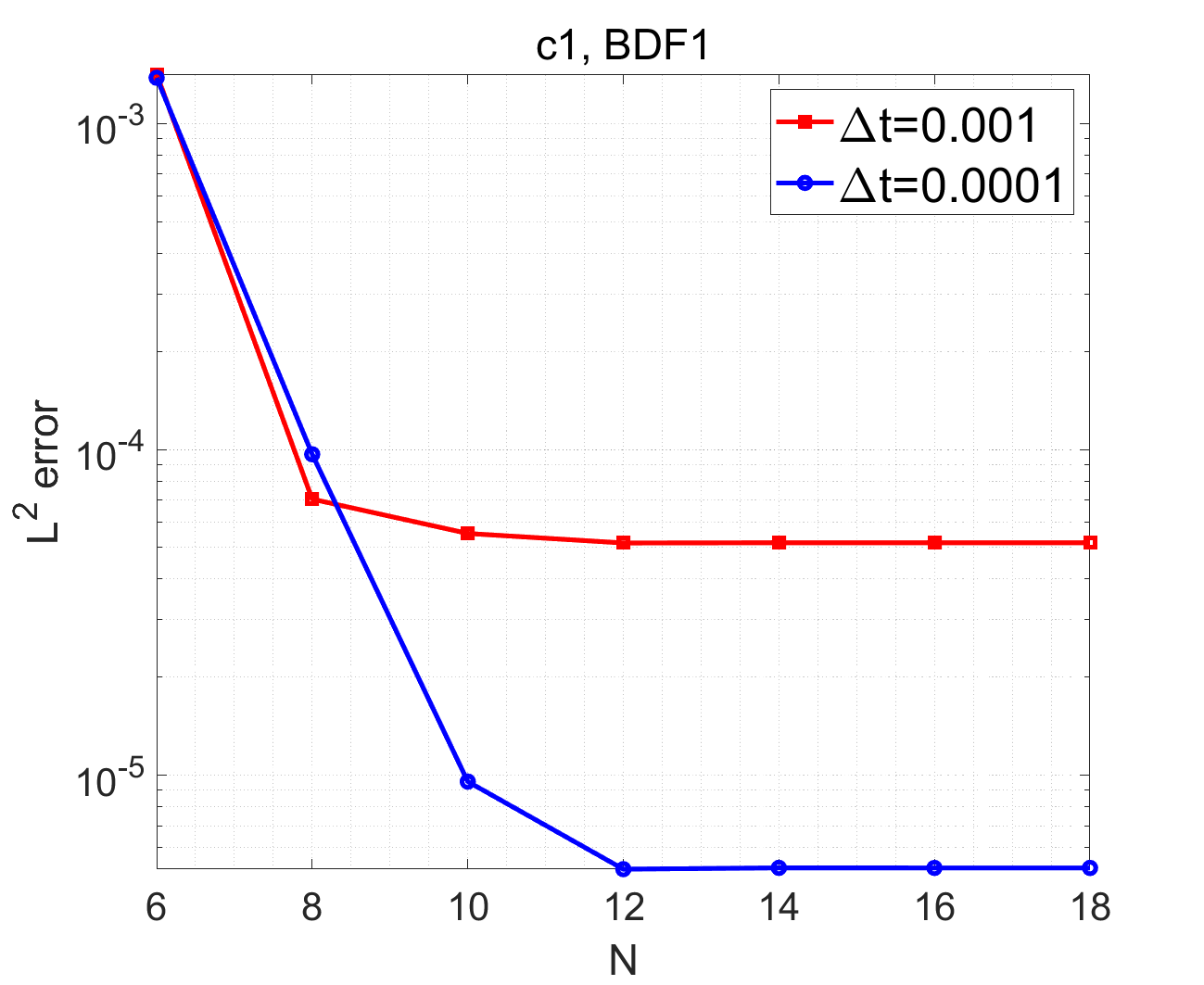
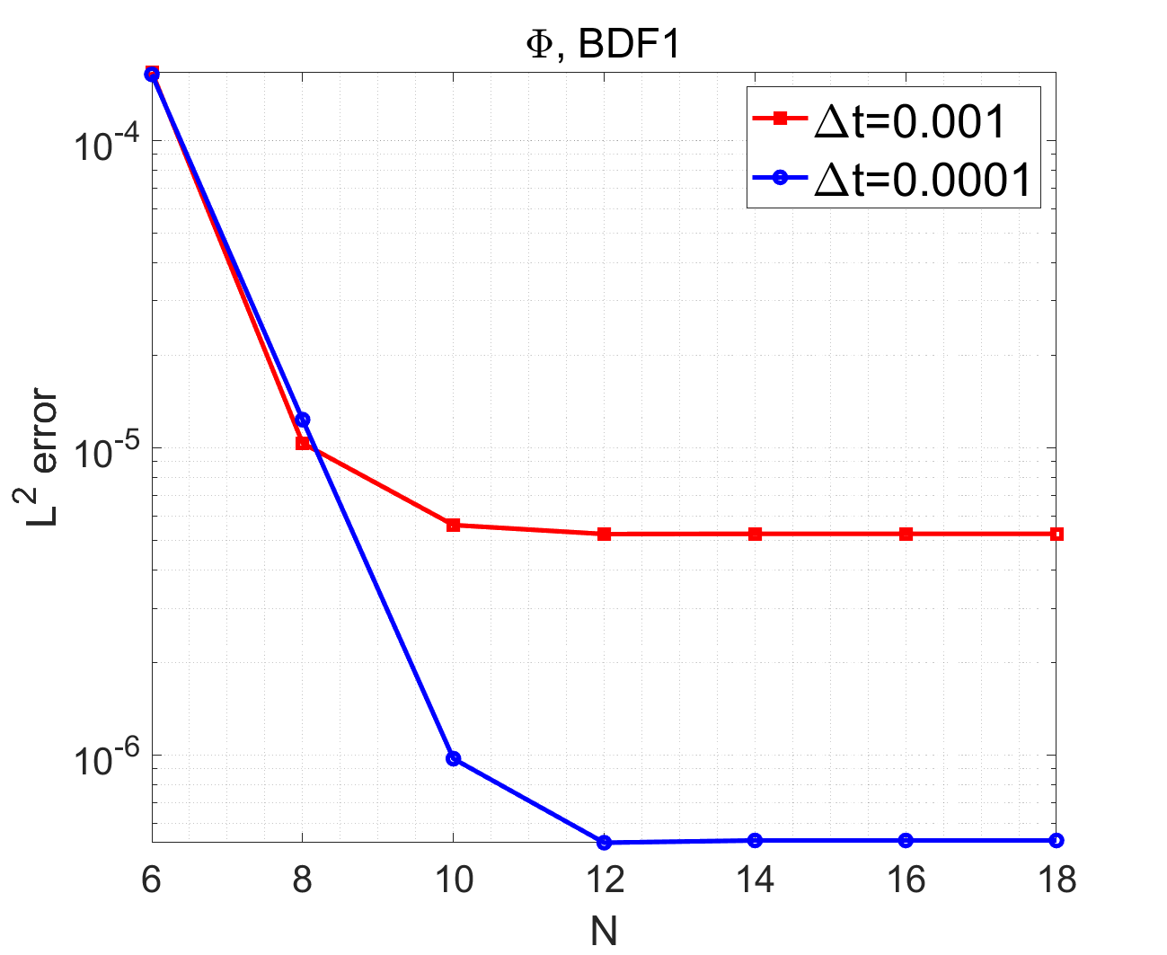
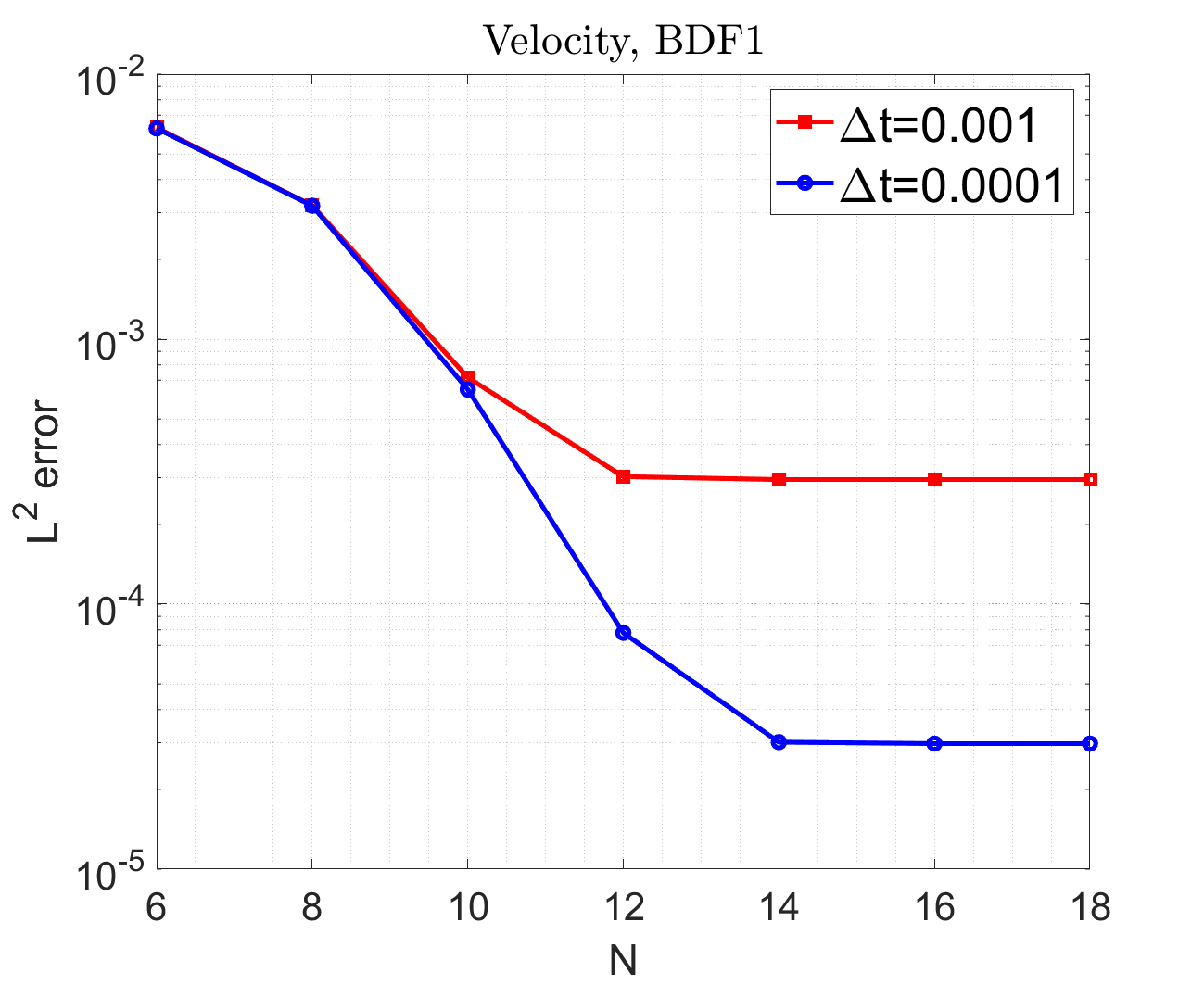
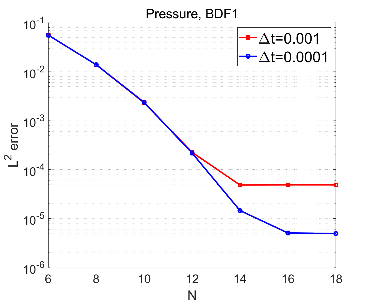
Figure 5.1. (Example 1) Errors in $L^{2}$-norm as functions of $N$ in semi-log scale for $\Delta t=0.001,\ 0.0001$ using the 1st-order scheme.

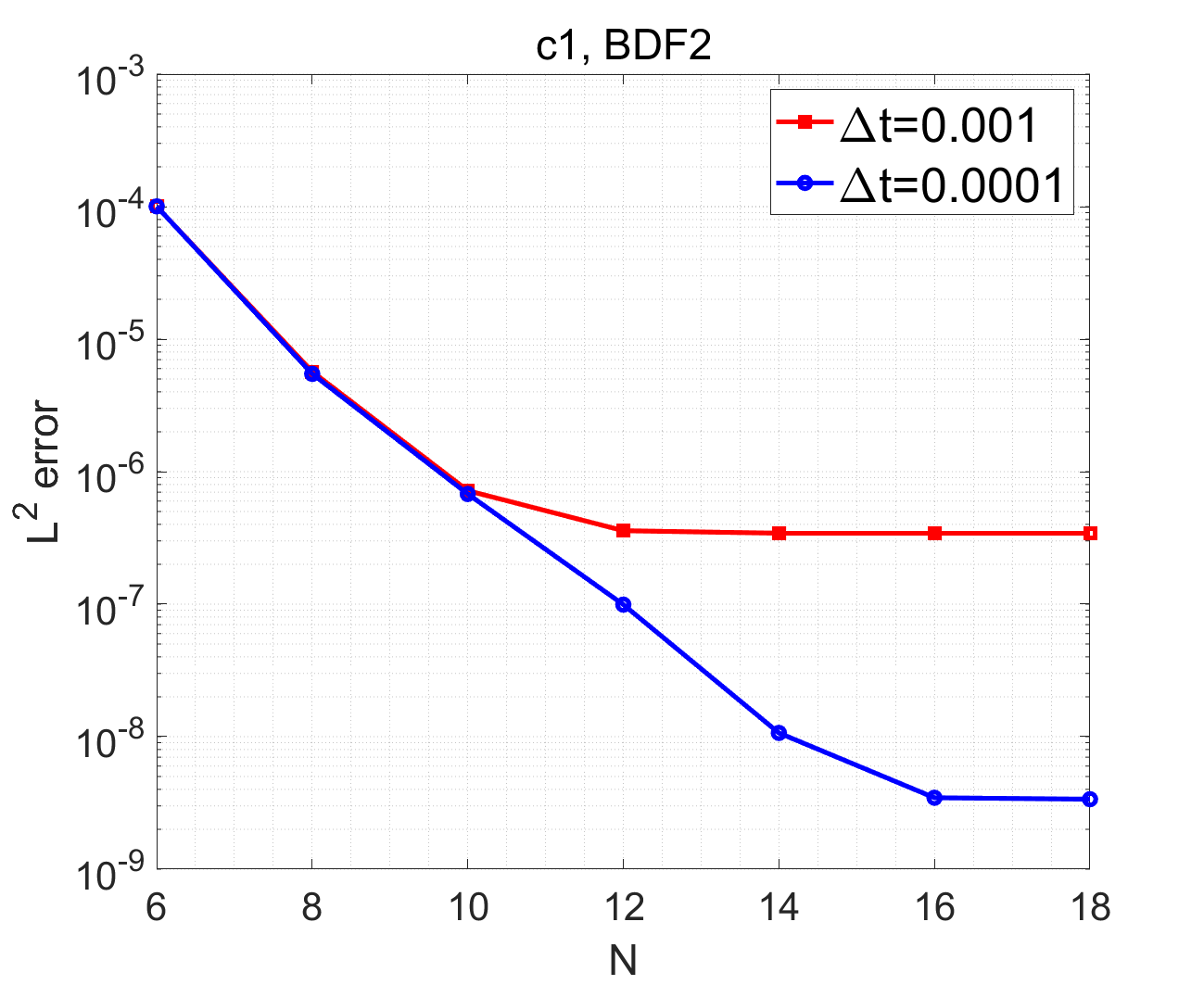
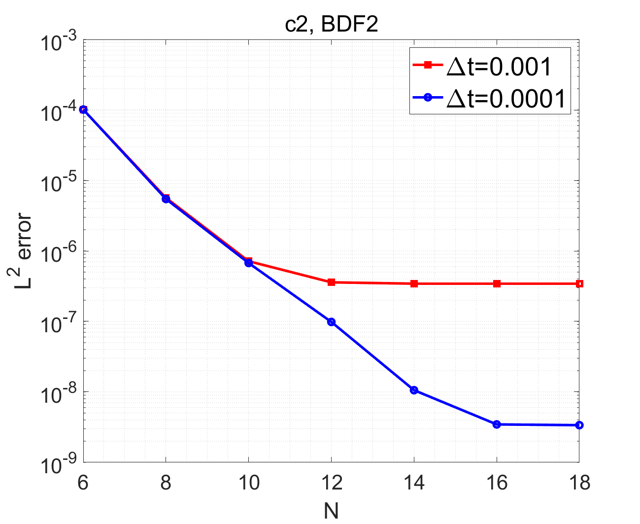
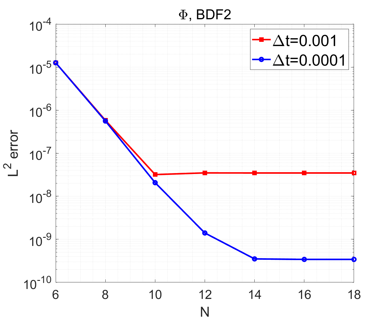
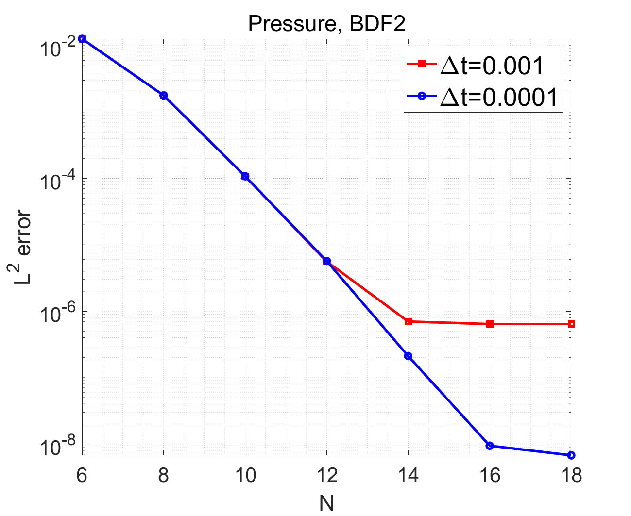
Figure 5.2. (Example 1) Errors in $L^{2}$-norm as functions of $N$ in semi-log scale for $\Delta t=0.001,\ 0.0001$ using the 2nd-order scheme.

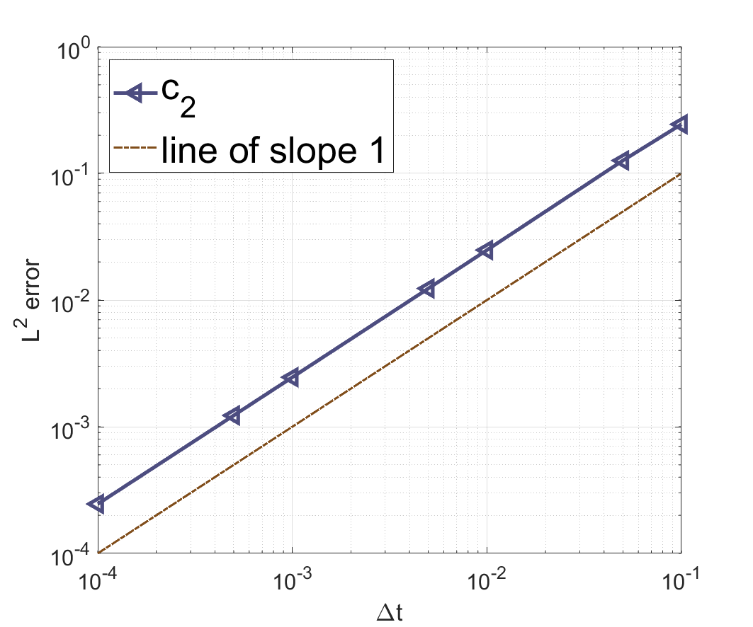
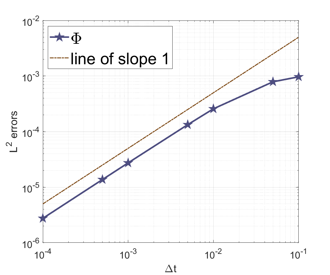
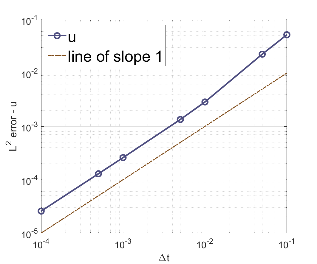
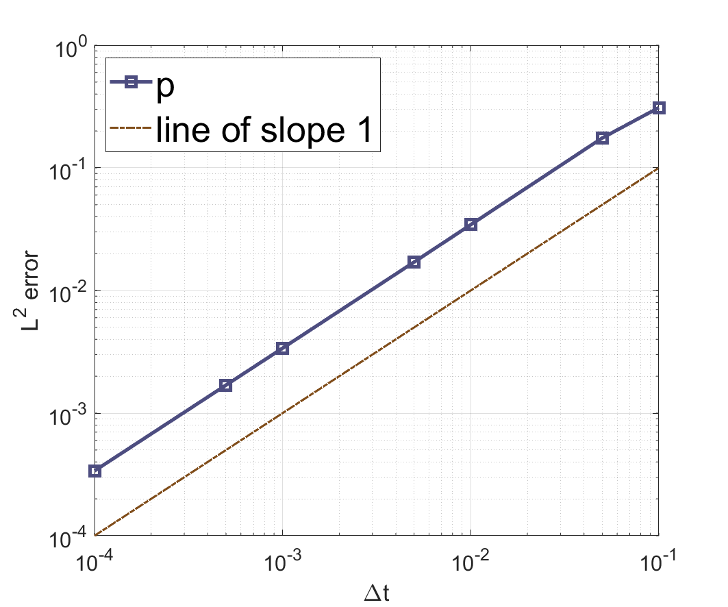
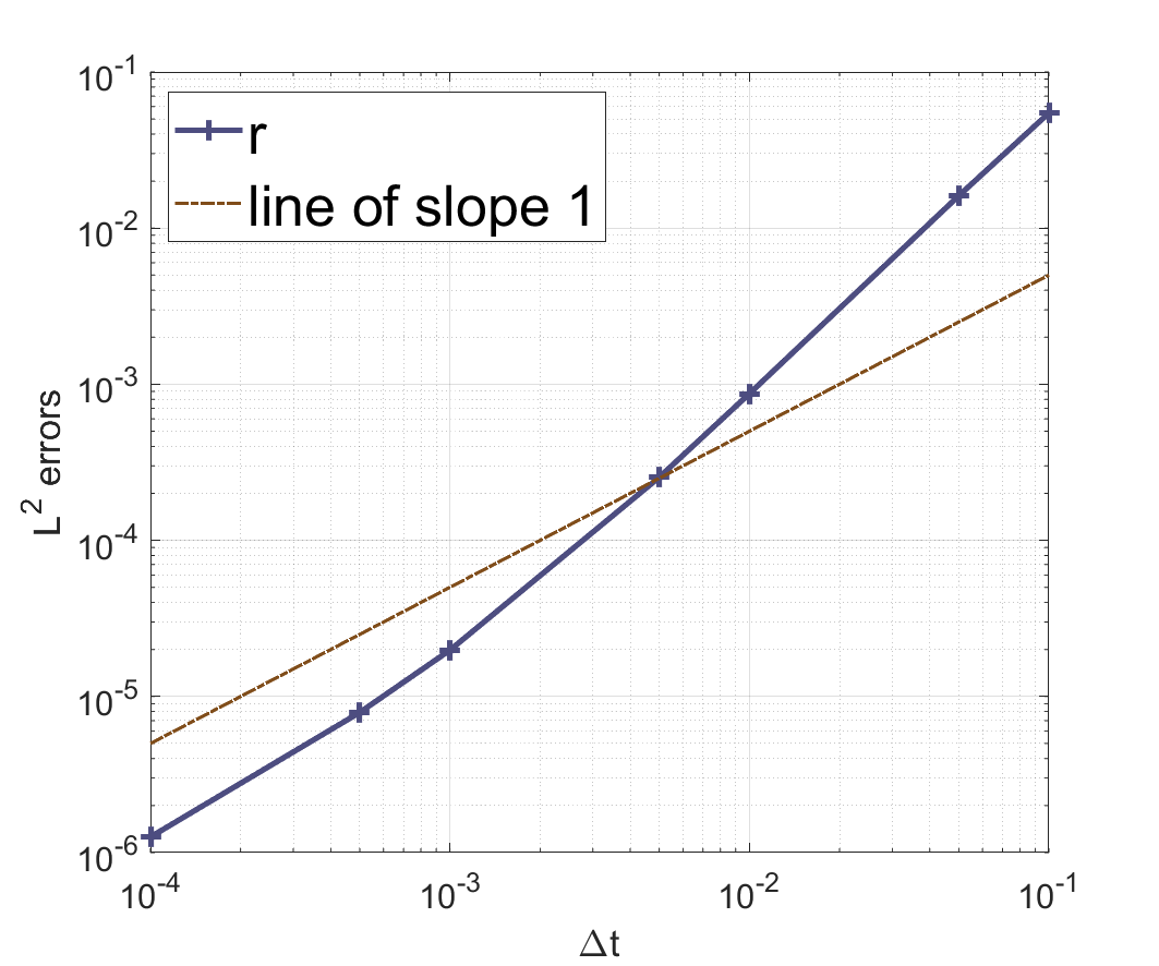
Figure 5.3. (Example 1) $L^{2}$-errors as a function of $\Delta t$ in log-log scale for the first order scheme.

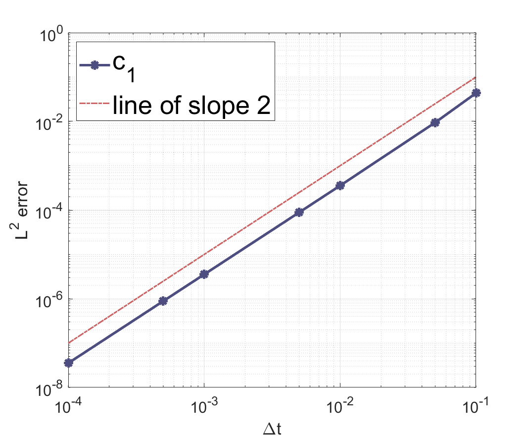
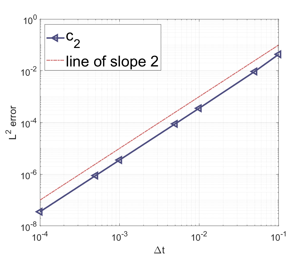
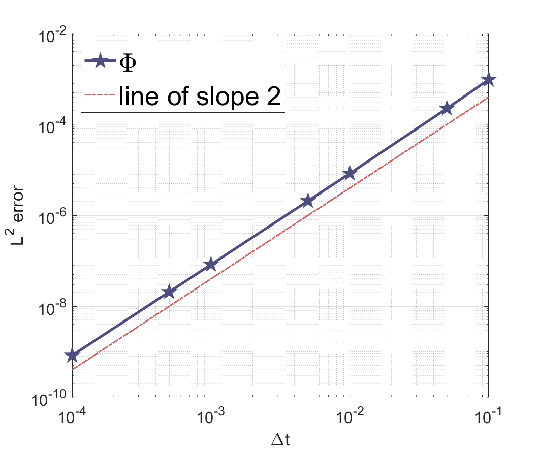
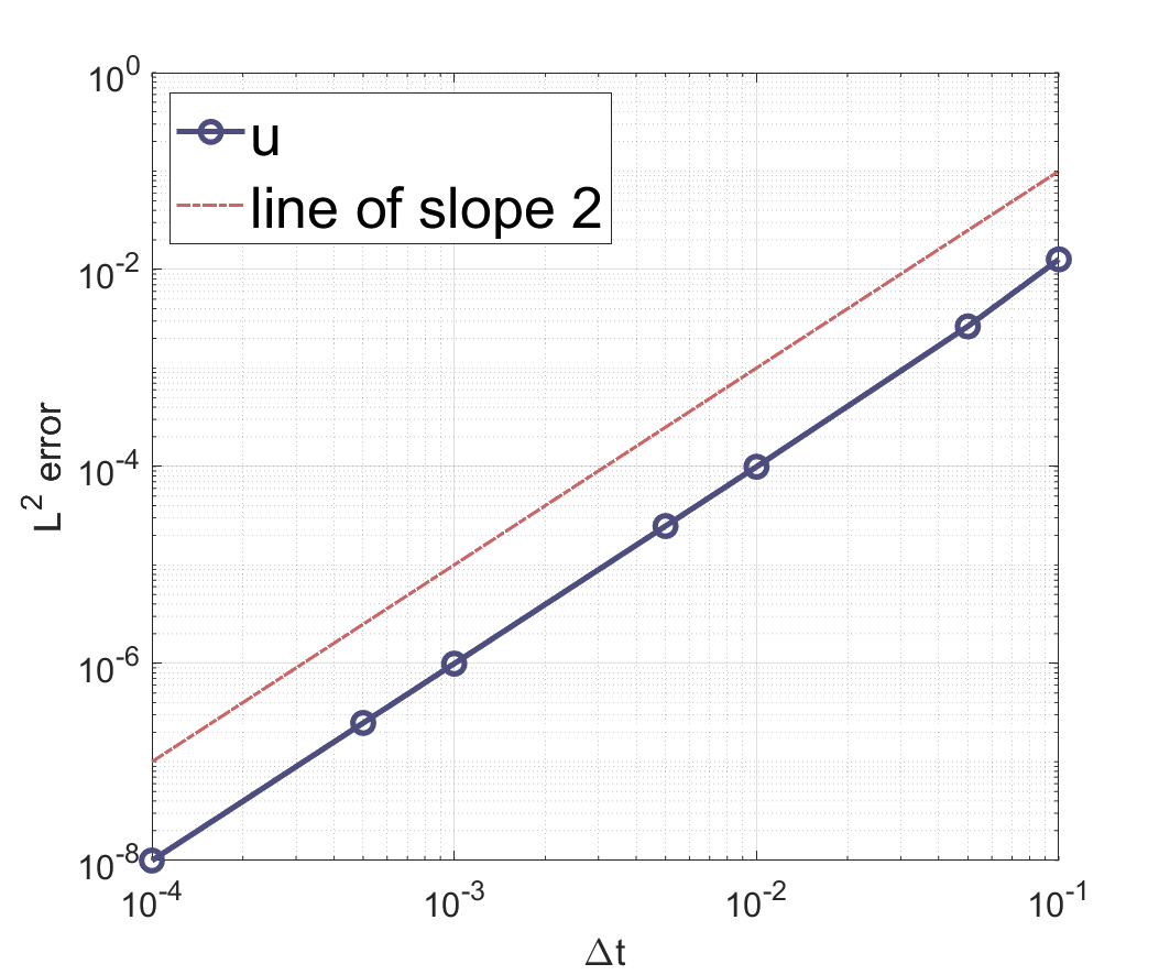
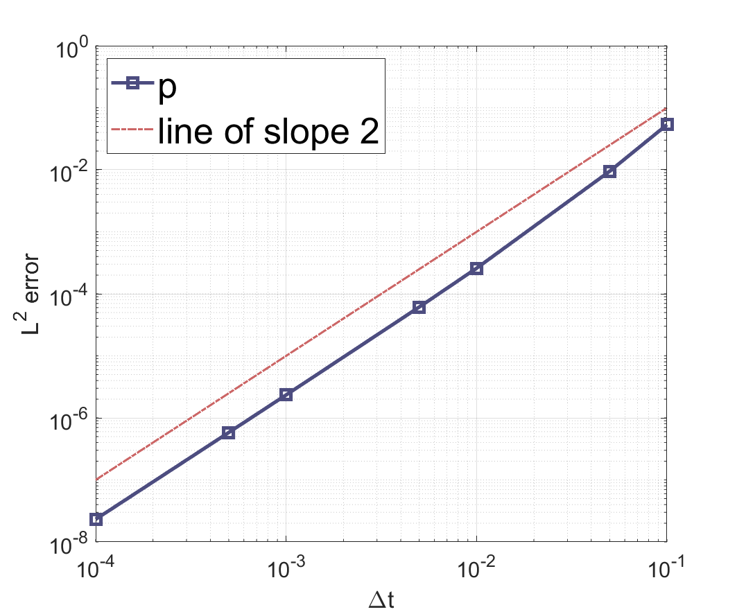
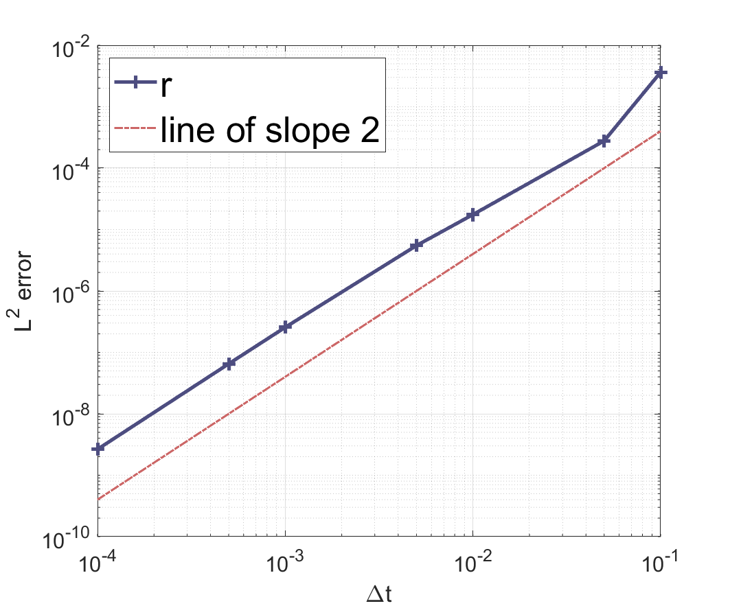
Figure 5.4. (Example 1) L2-errors as functions of $\Delta t$ in log-log scale for the second order scheme.

Table 5.1. Velocity $L^{2}$-error and pressure $L^{2}$-error with respect to time step size at $T=1$, computed by Scheme2-SM and Scheme2b-SM, respectively.

$\Delta t$	$L^{2}$ velocity error		$L^{2}$ pressure error
	Scheme2-SM	Scheme2b-SM	Scheme2-SM	Scheme2b-SM
$10^{-1}$	1.26768E-02	1.26935E-02	5.33609E-02	5.33894E-02
$10^{-2}$	9.92445E-05	9.90649E-05	2.58586E-04	2.57952E-04
$10^{-3}$	9.92721E-07	9.92952E-07	2.34312E-06	2.34164E-06
$10^{-4}$	9.93110E-09	9.93277E-09	2.31898E-08	2.31877E-08

An accuracy comparison between Scheme2-SM and Scheme2b-SM is given in Table 5.1. The velocity $L^{2}$-error and pressure $L^{2}$-error listed in the table indicates that the two schemes are almost equal in term of the accuracy. The error comparison for the other variables (not shown here) has given similar results.

Example 2

Set $z_{1}=1,z_{2}=-1,D_{1}=D_{2}=1$, $\epsilon=1$, $\nu=0.01$, and $N=64$. This example has a purpose to verify the positivity preserving, mass conserving and stability property. We run Scheme2b-SM with the initial conditions:

$$\mathbf{u}({\boldsymbol{x}},0)=(\pi{\sin}(2\pi y){\sin}^{2}(\pi x),-\pi\sin(2\pi x){\sin}^{2}(\pi y))$$

$$c_{1}({\boldsymbol{x}},0)=1.1+\cos(\pi x)\cos(\pi y)$$

$$c_{2}({\boldsymbol{x}},0)=1.1-\cos(\pi x)\cos(\pi y).$$

Figure 5.5 plots time evolution of the discrete masses $\int_{\Omega}c_{i}d{\boldsymbol{x}},\ i=1,2$ computed by using Scheme2b-SM, which demonstrates the mass conservation property of the scheme. Figures 5.6 - 5.9 present the snapshots at $t=0,\ 0.1,\ 0.6,\ 1.0$ of the variables $c_{1},\ c_{2}$, and two components of the velocity $u_{1}$ and $u_{2}$, respectively. It is observed from Figures 5.6 and 5.7 that the concentrations $\{c_{i}\}$ preserve the positivity during the time evolution.

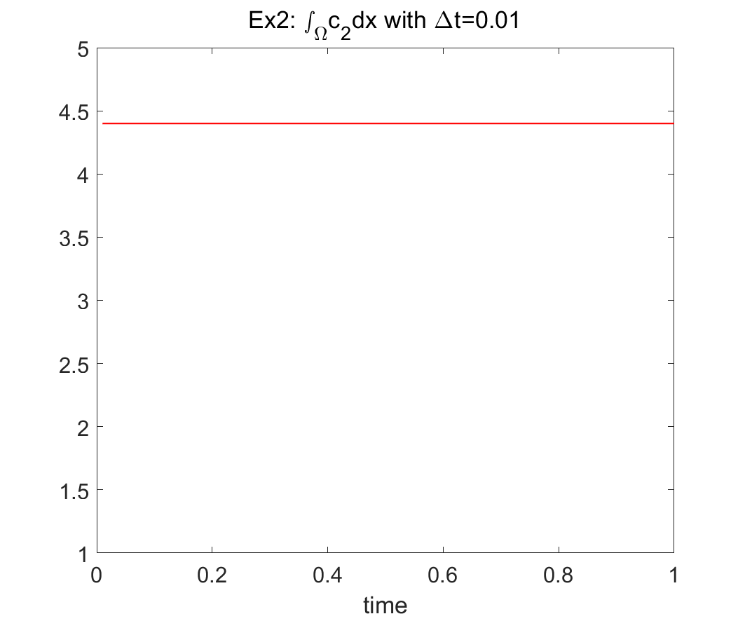
Figure 5.5. (Example 2) Time evolution of the discrete mass $\int_{\Omega}c_{1}d{\boldsymbol{x}}$ (a) and $\int_{\Omega}c_{2}d{\boldsymbol{x}}$ (b) computed with Scheme2b-SM.

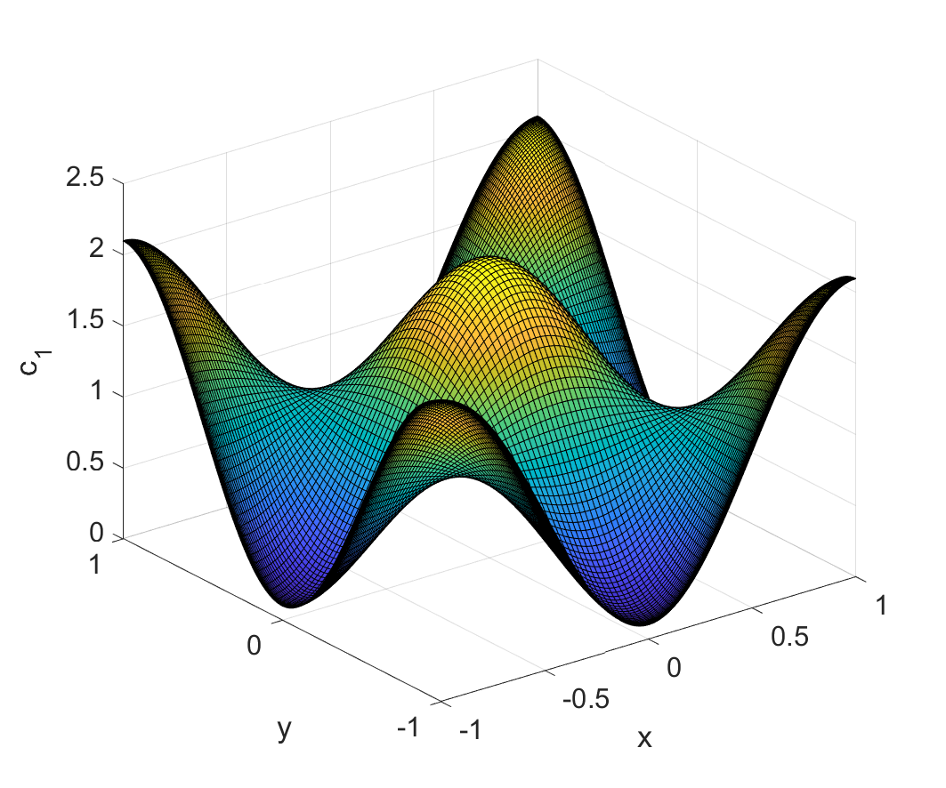
(a) $c_{1}$ at $t=0$

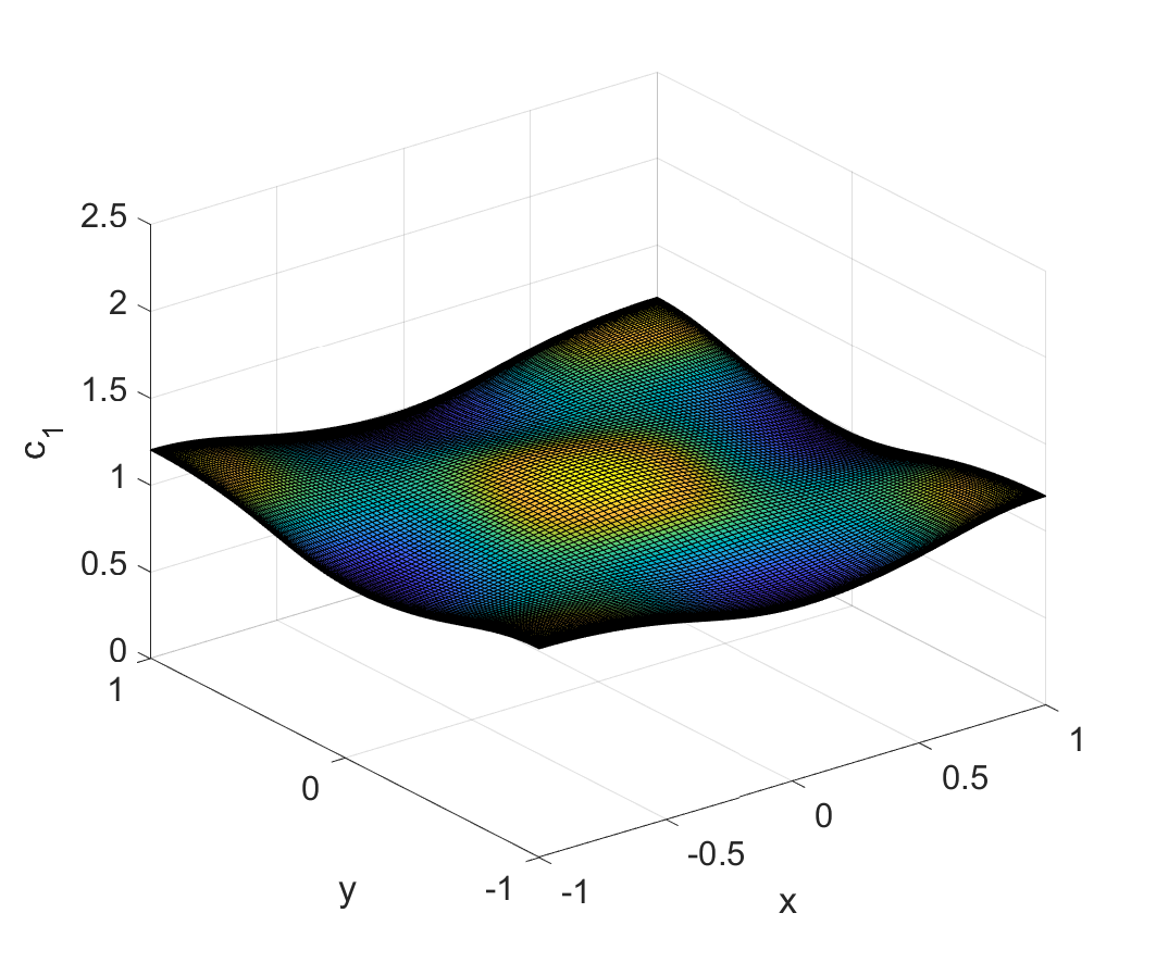
(b) $c_{1}$ at $t=0.1$

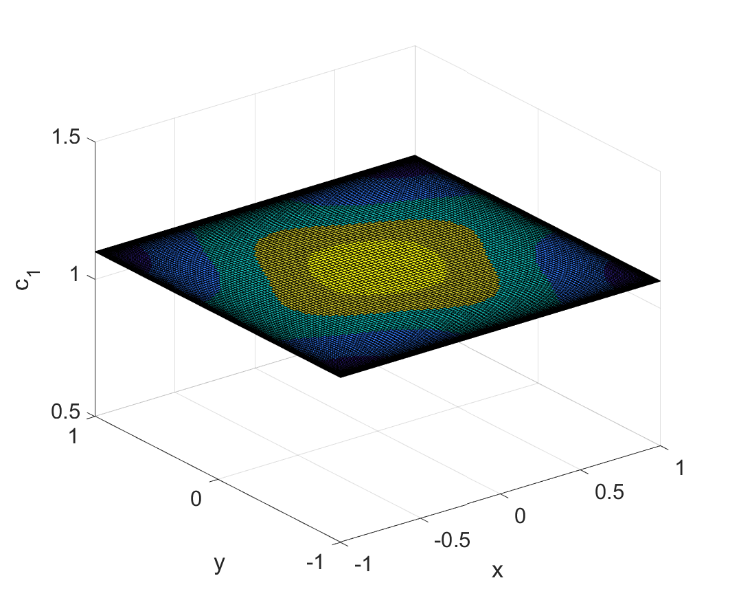
(c) $c_{1}$ at $t=0.6$

(d) $c_{1}$ at $t=1$

Figure 5.6. (Example 2) Snapshots of $c_{1}$.

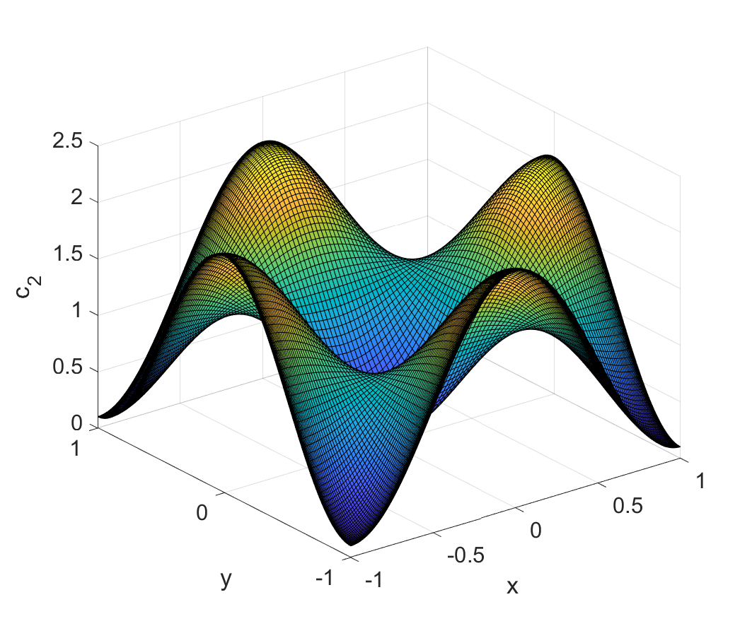
(a) $c_{2}$ at $t=0$

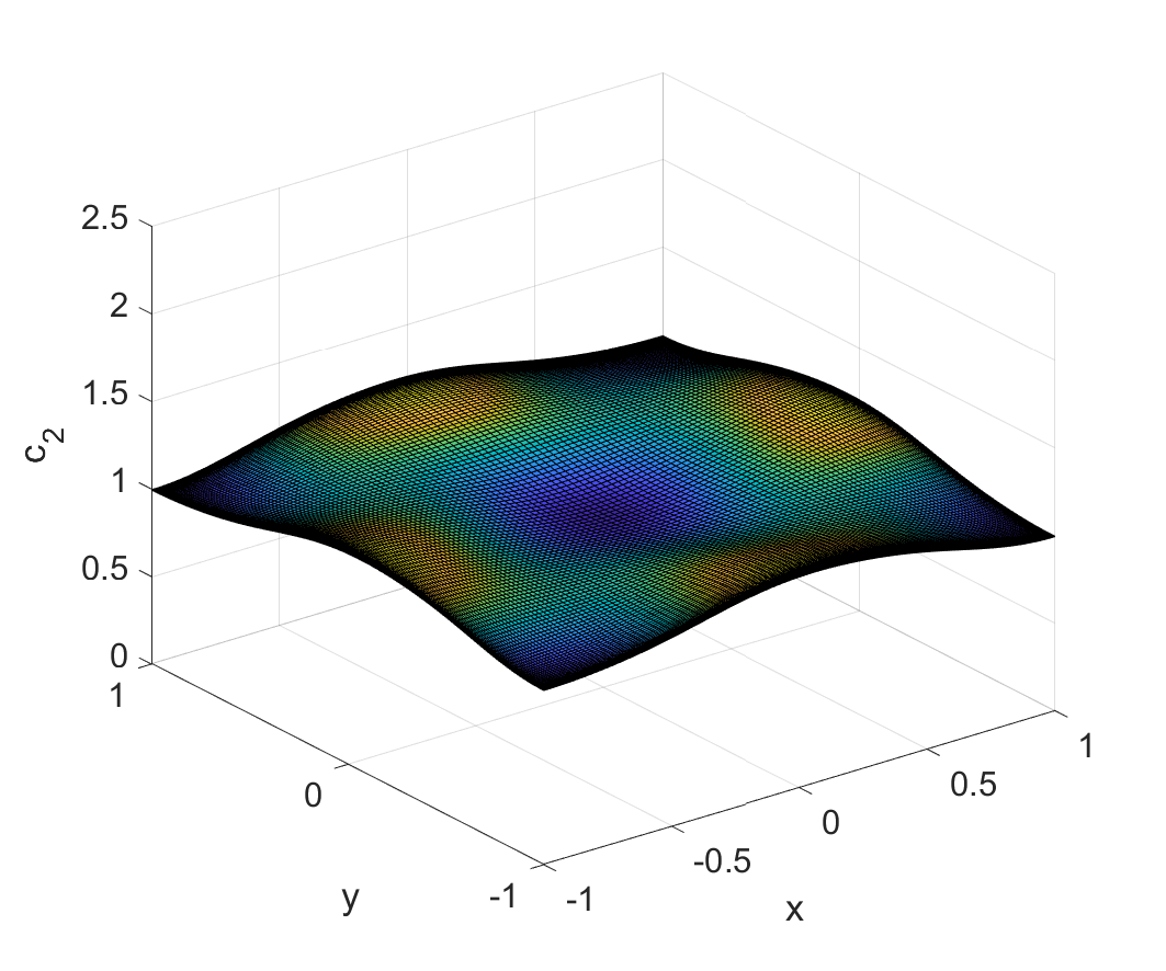
(b) $c_{2}$ at $t=0.1$

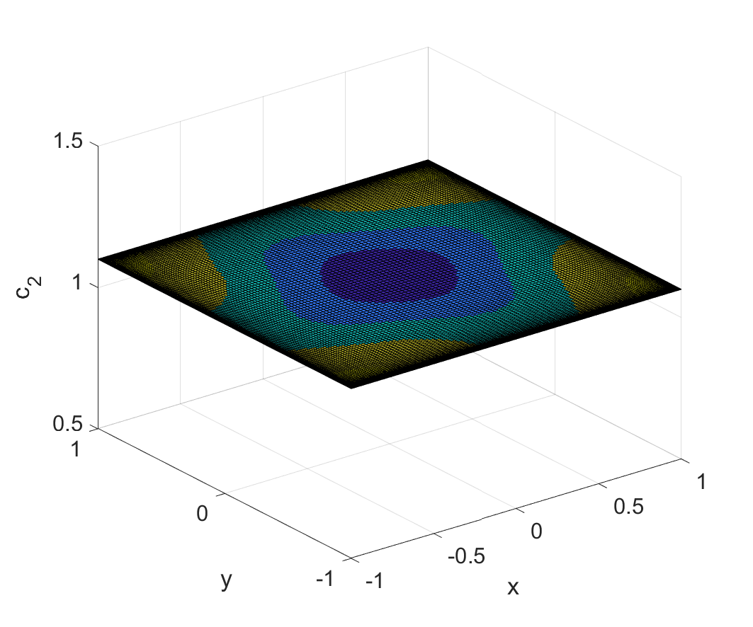
(c) $c_{2}$ at $t=0.6$

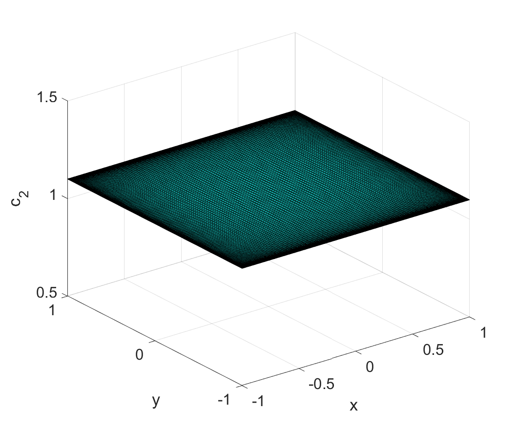
(d) $c_{2}$ at $t=1$

Figure 5.7. (Example 2) Snapshots of $c_{2}$.

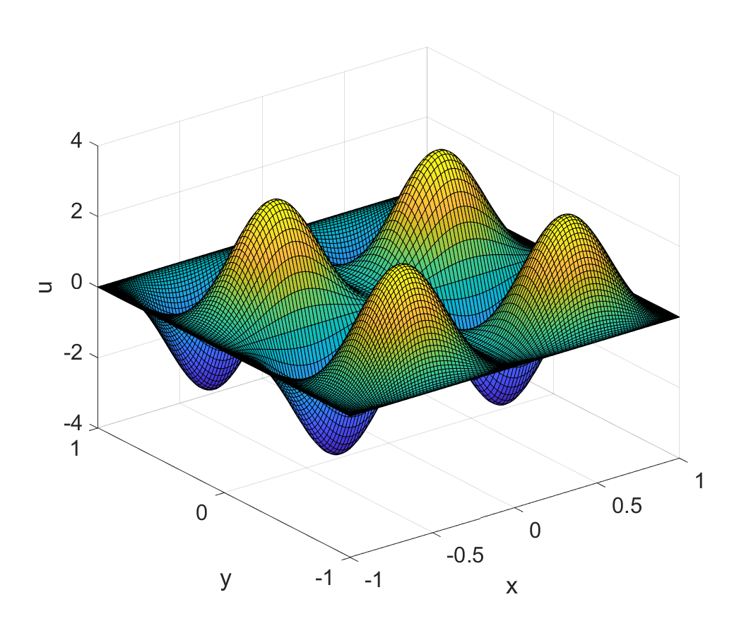
(a) $u_{1}$ at $t=0$

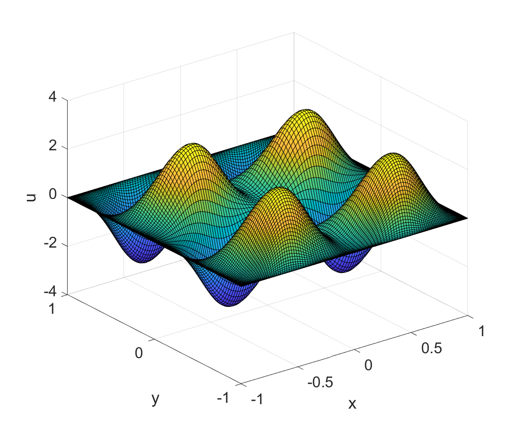
(b) $u_{1}$ at $t=0.1$

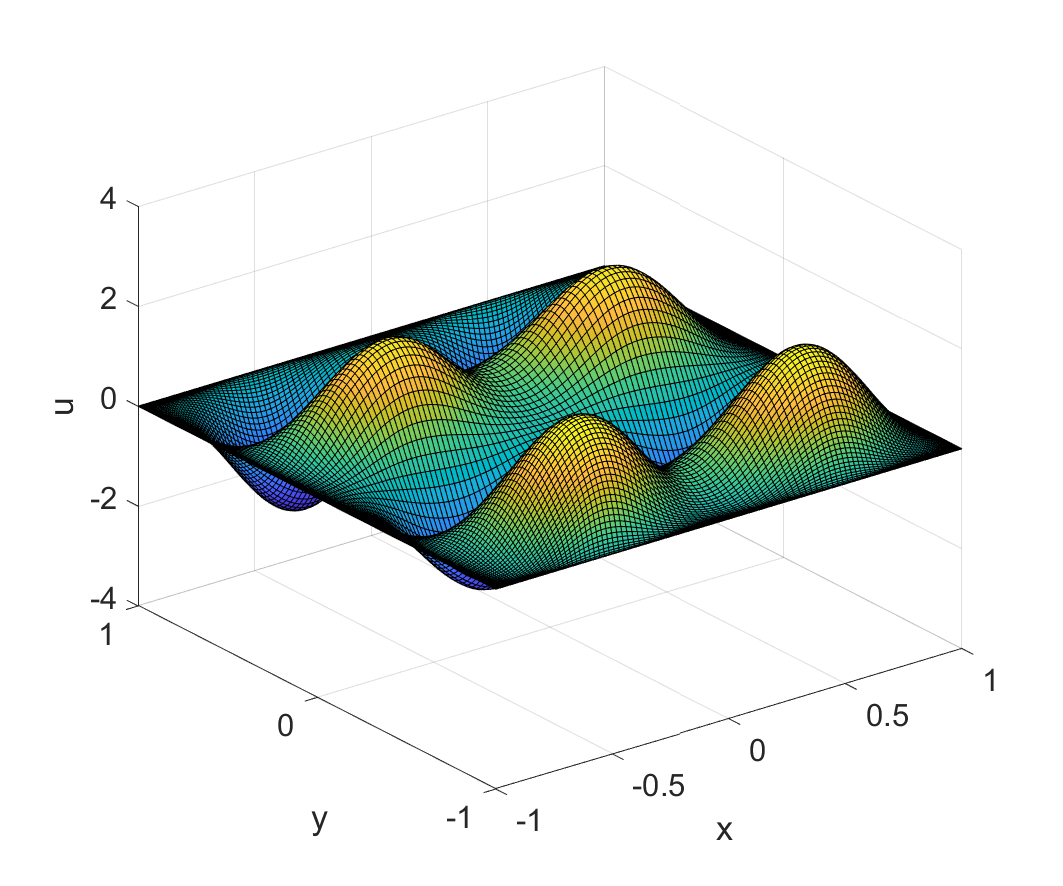
(c) $u_{1}$ at $t=0.6$

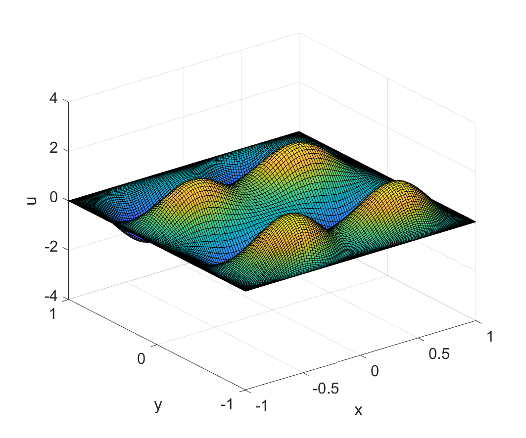
(d) $u_{1}$ at $t=1$

Figure 5.8. (Example 2) Snapshots of $u_{1}$.

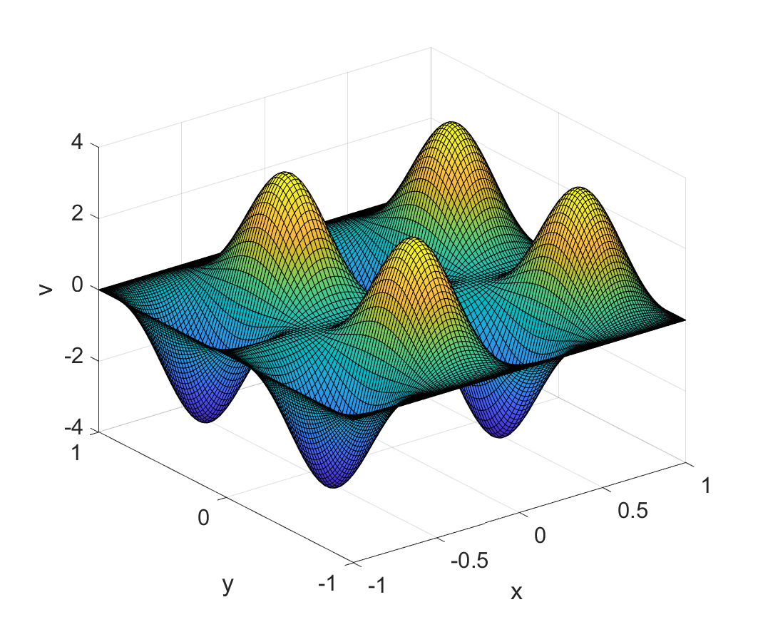
(a) $u_{2}$ at $t=0$

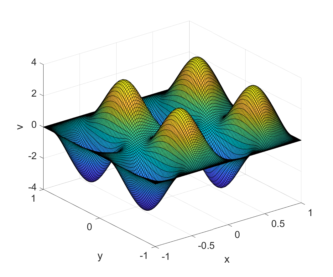
(b) $u_{1}$ at $t=0.1$

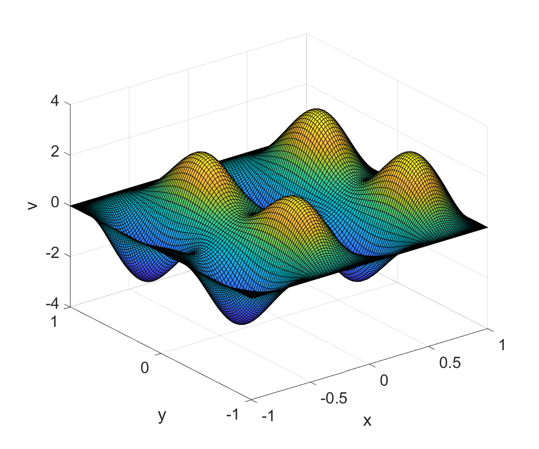
(c) $u_{2}$ at $t=0.6$

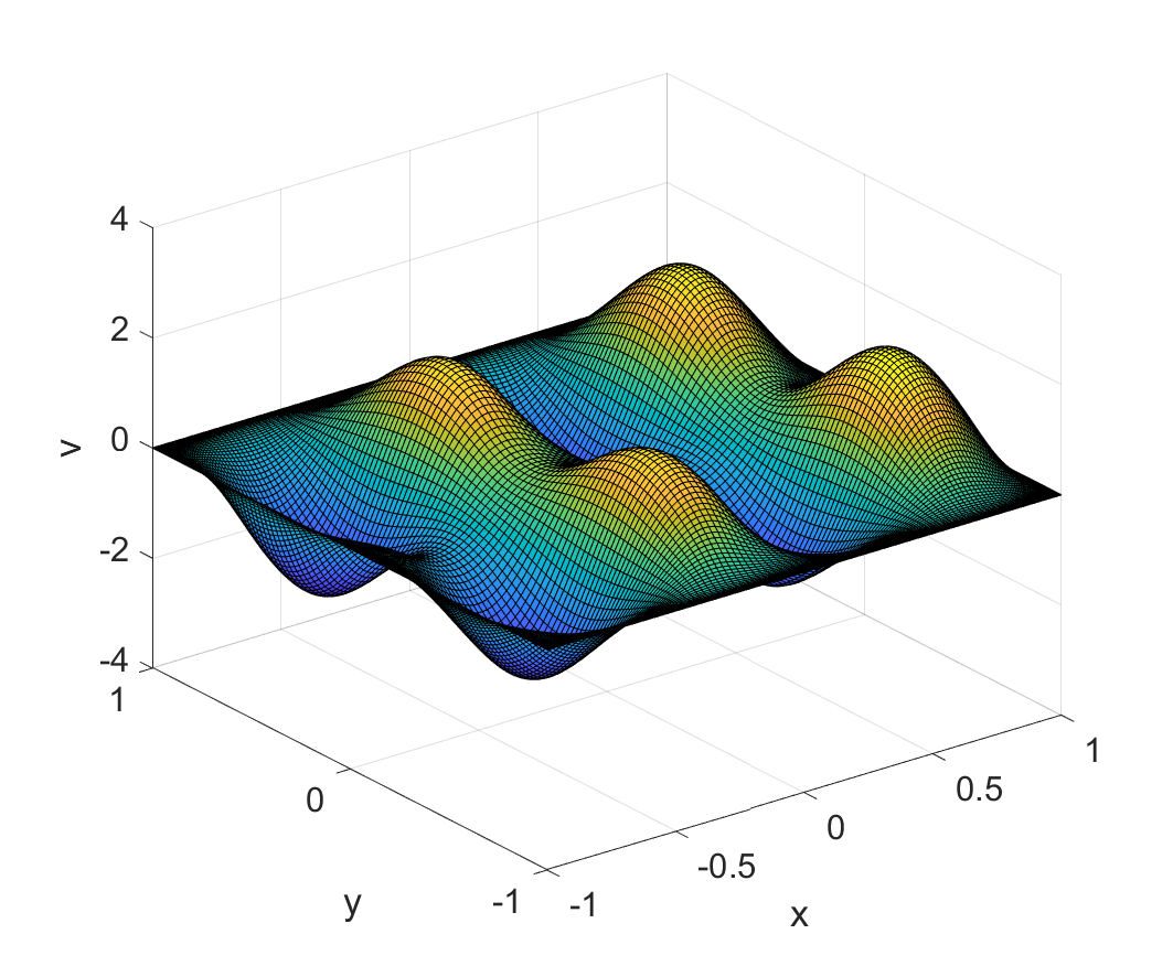
(d) $u_{2}$ at $t=1$

Figure 5.9. (Example 2) Snapshots of $u_{2}$ .

5.2. Case with three ions

Example 3

Set $z_{1}=1,z_{2}=-1,z_{3}=2,D_{1}=D_{2}=D_{3}=1,\epsilon=0.5,\ \nu=0.1$, we verify the temporal convergence rates of the proposed schemes using the following fabricated exact solution:

$$\mathbf{u}=(\pi{\sin}(2\pi y){\sin}^{2}(\pi x),-\pi\sin(2\pi x){\sin}^{2}(\pi y))e^{-t}$$

$$p=\sin(\pi x)\sin(\pi y)e^{-t}$$

$$c_{1}=\cos(\pi x)\cos(\pi y)e^{-t}+2e^{-t}$$

$$c_{2}=-2\cos(\pi x)\cos(\pi y)e^{-t}+6e^{-t}$$

$$c_{3}=-\cos(\pi x)\cos(\pi y)e^{-t}+2e^{-t}$$

$$\Phi=\frac{1}{\pi^{2}}\cos(\pi x)\cos(\pi y)e^{-t}.$$

The source terms are obtained from the exact solution. Figures 5.10 and 5.11 present the $L^{2}$ errors of the ions, the electrostatic potential, the velocity, and the pressure as functions of the time step size, computed from Scheme1-SM and Scheme2-SM respectively. As observed from the figures, the convergence rates are respectively first order for Scheme1-SM and second order for Scheme2-SM. This in a good agreement with the theoretical prediction.

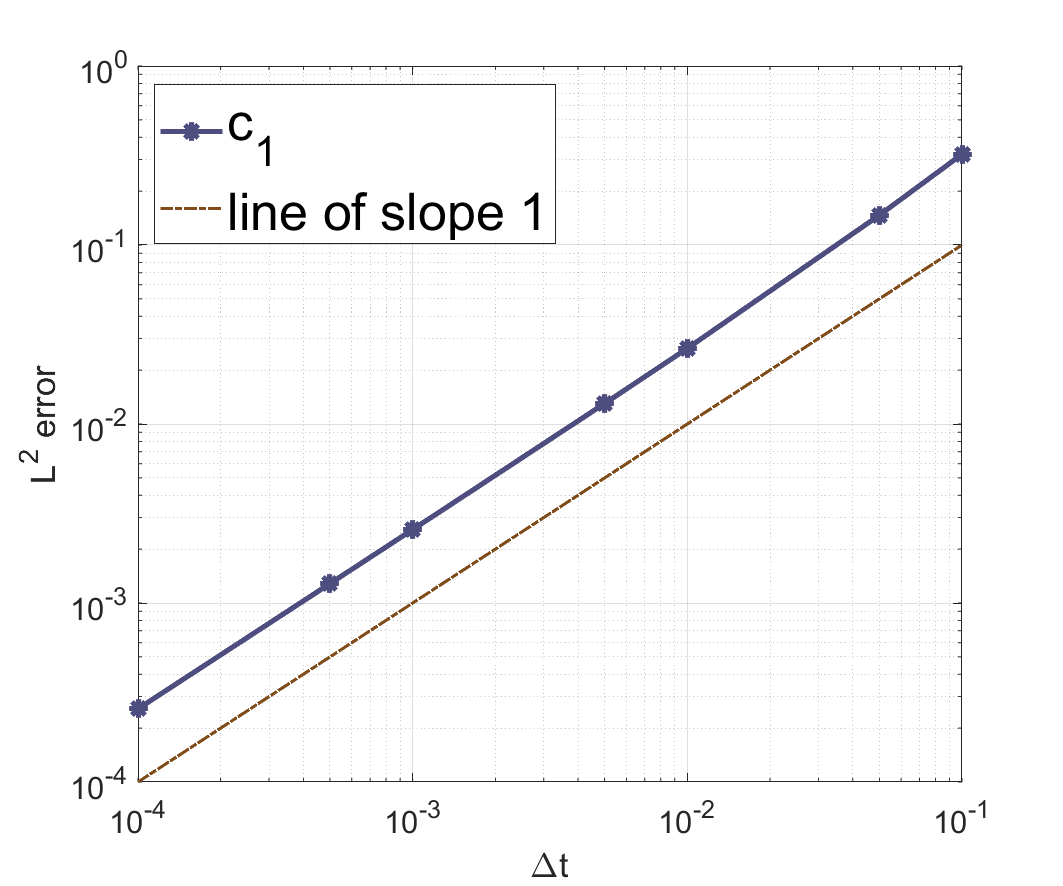
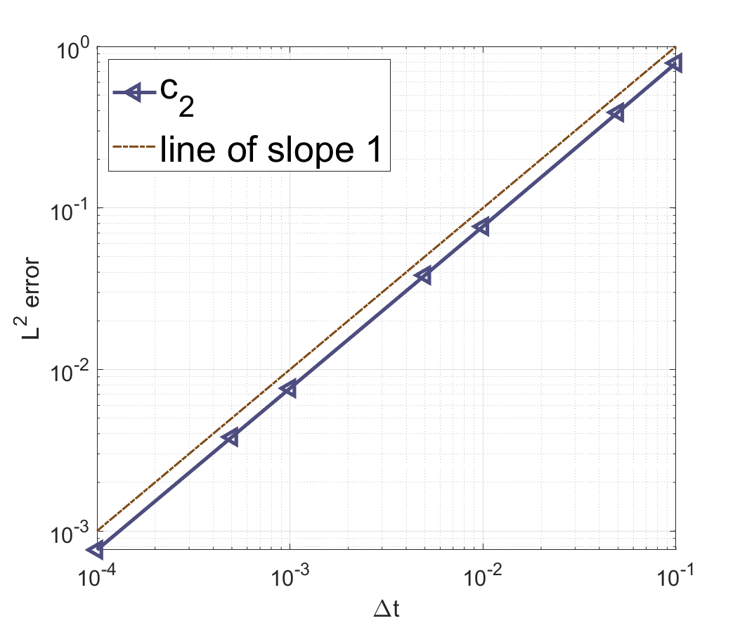
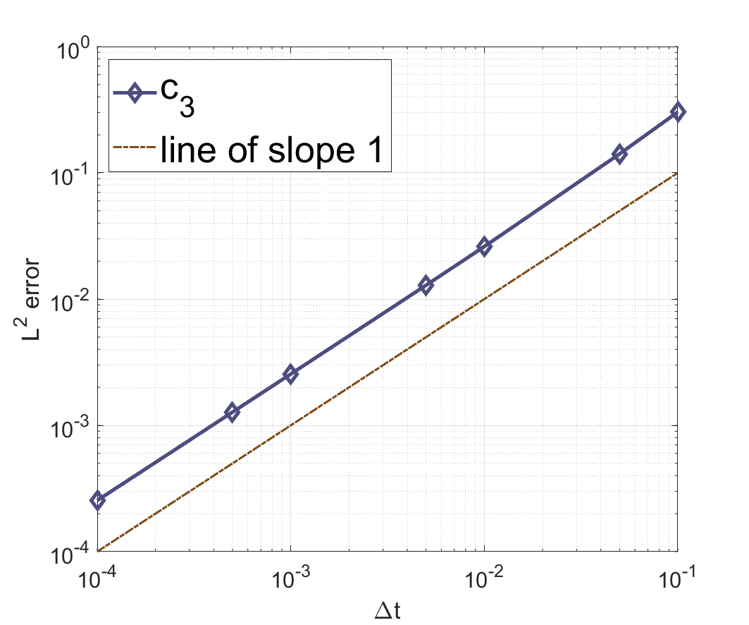
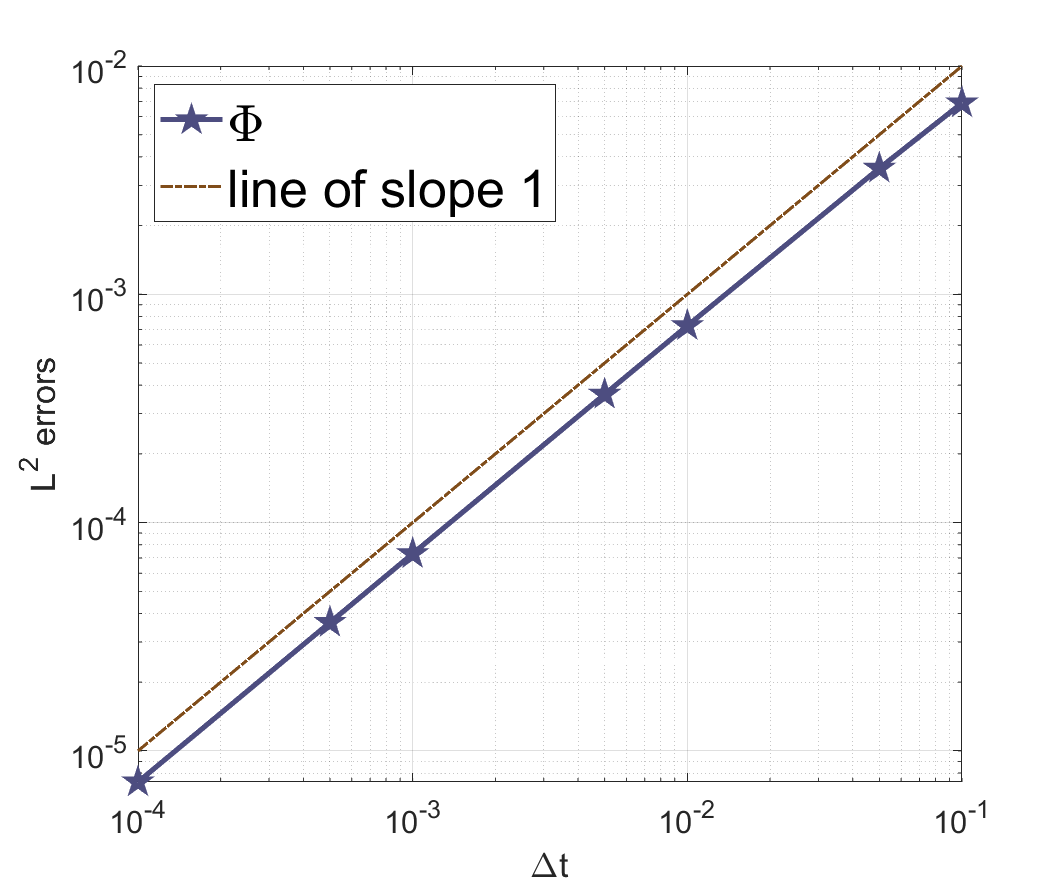
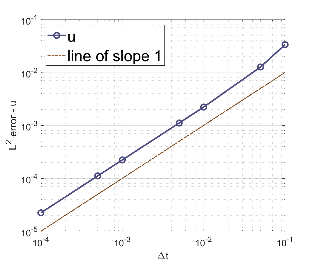
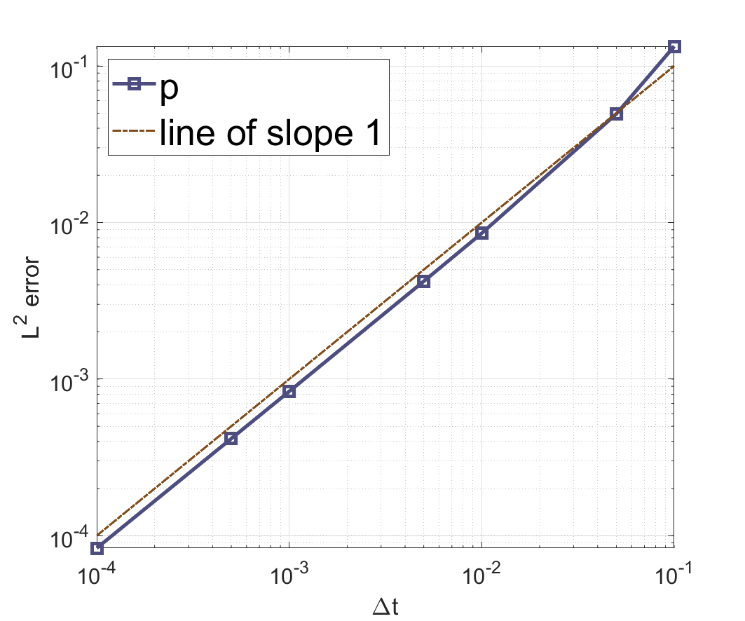
Figure 5.10. (Example 3) $L^{2}$ error versus $\Delta t$ in log-log scale using the first order scheme with $N=64$ at each spatial direction.

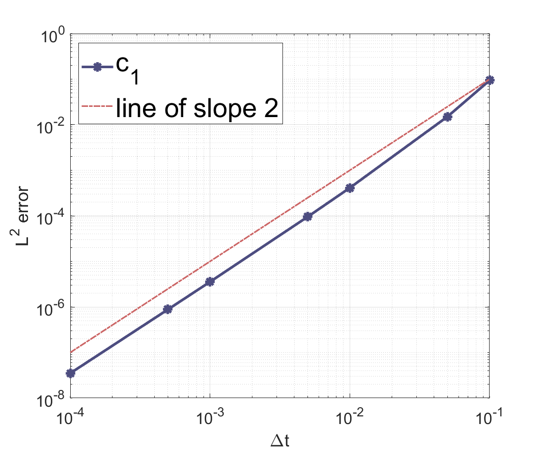
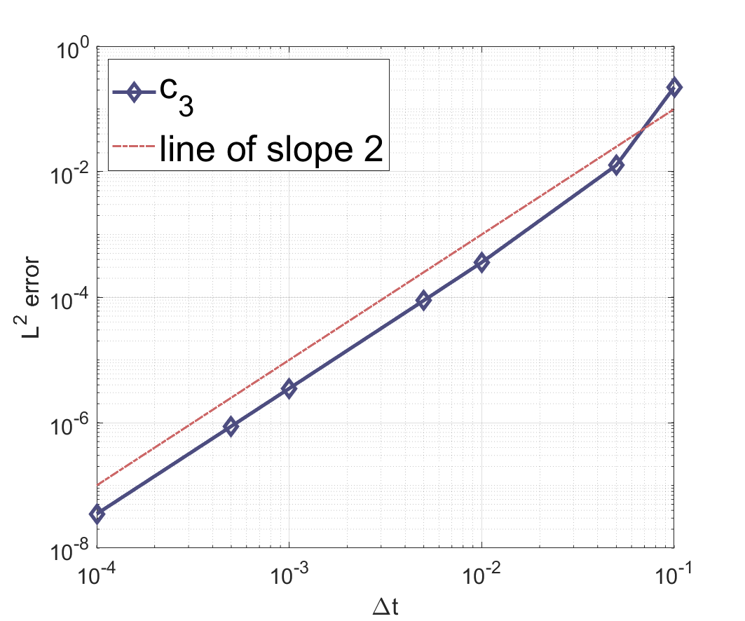
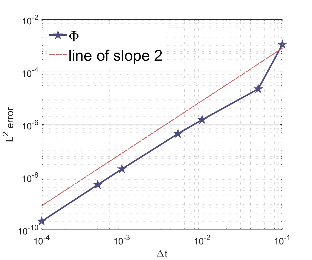
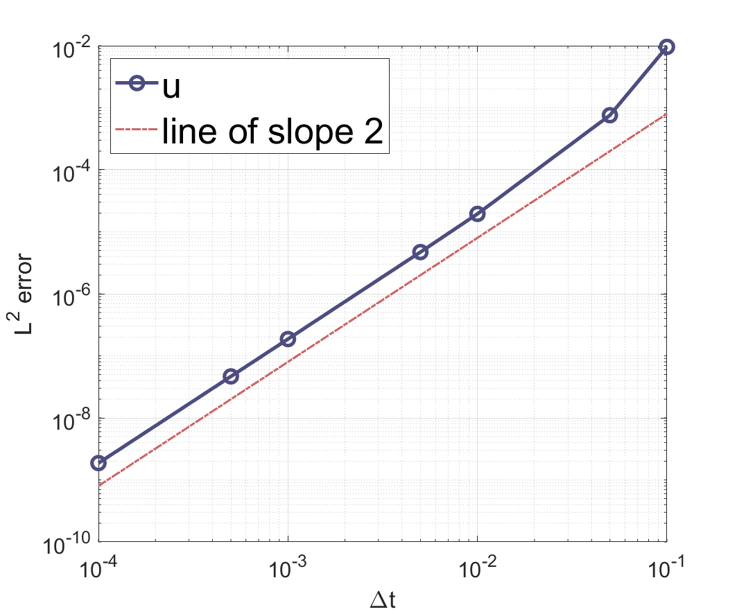
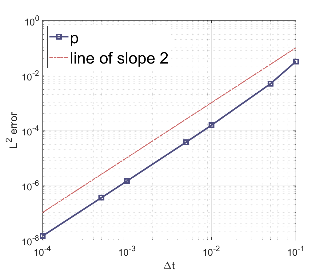
Figure 5.11. (Example 3) $L^{2}$ errors versus $\Delta t$ in log-log scale using Scheme2-SM with $N=64$ at each spatial direction.

6. Concluding Remarks

In this paper, we have developed efficient time-stepping schemes for the Navier-Stokes-Nernst-Planck-Poisson equations. The proposed schemes are constructed based on an auxiliary variable approach for the Navier-Stokes equations and a delicate treatment of the terms coupling the Navier-Stokes equations and the Nernst-Planck-Poisson equations. By introducing a dynamic equation for the auxiliary variable and reformulating the original equations into an equivalent system, we have constructed first- and second-order semi-implicit linearized schemes for the underlying problem. A rigorous analysis was carried out, showing that the overall schemes are unconditionally stable, and preserve positivity and mass conservation of the ionic concentration solutions. The implementation showed that it can be implemented in an efficient way: the computational complexity is equal to solving several decoupled linear equations with constant coefficient at each time step. A number of numerical examples were provided to confirm the theoretical claims. We emphasize that the above attractive properties remain to be held at the full discrete level. As far as the best we know, this is the first second-order method which satisfies all the above properties for the Navier-Stokes-Nernst-Planck-Poisson equations at the discrete level.

References

- [1] L. Angermann and S. Wang, Three-dimensional exponentially fitted conforming tetrahedral finite elements for the semiconductor continuity equations, Appl. Numer. Math., 46 (2003), pp. 19–43.
- [2] M. Bazant, K. Thornton, and A. Ajdari, Diffuse-charge dynamics in electrochemical systems, Phys. Rev. E, 70 (2004), p. 021506.
- [3] D. Bothe, A. Fischer, and J. Saal, Global well-posedness and stability of electrokinetic flows, SIAM J. Math. Anal., 46 (2014), pp. 1263–1316.
- [4] A. Bousquet, X. Hu, M. S. Metti, and J. Xu, Newton solvers for drift-diffusion and electrokinetic equations, SIAM J. Sci. Comput., 40 (2018), pp. B982–B1006.
- [5] Q. Cheng and J. Shen, Multiple scalar auxiliary variable (MSAV) approach and its application to the phase–field vesicle membrane model, SIAM J. Sci. Comput., 40 (2018), pp. A3982–A4006.
- [6] Q. Cheng and J. Shen, Global constraints preserving scalar auxiliary variable schemes for gradient flows, SIAM J. Sci. Comput., 42 (2020), pp. A2489–A2513.
- [7] P. Constantin and M. Ignatova, On the Nernst-Planck-Navier-Stokes system, Arch. Rational Mech. Anal., 232 (2018), pp. 1379–1428.
- [8] P. Constantin, M. Ignatova, and F.-N. Lee, Nernst-Planck-Navier-Stokes systems near equilibrium, preprint, (2020).
- [9] C. Deng, J. Zhao, and S. Cui, Well-posedness for the Navier-Stokes-Nernst-Planck-Poisson system in Triebel-Lizorkin space and Besov space with negative indices, J. Math. Anal. Appl., 377 (2011), pp. 392–405.
- [10] J. Guermond and J. Shen, On the error estimates for the rotational pressure-correction projection methods, Math. Comput., 73 (2004), pp. 1719–1737.
- [11] M. He and P. Sun, Mixed finite element analysis for the Poisson-Nernst-Planck/Stokes coupling, J. Comput. Appl. Math., 341 (2018), pp. 61–79.
- [12] D. Hou, M. Azaïıez, and C. Xu, A variant of scalar auxiliary variable approaches for gradient flows, J. Comput. Phys., 395 (2019), pp. 307–332.
- [13] F. Huang and J. Shen, Bound/positivity preserving and energy stable scalar auxiliary variable schemes for dissipative systems: Applications to Keller-Segel and Poisson-Nernst-Planck equations, SIAM J. Sci. Comput., 43 (2021), pp. A1832–A1857.
- [14] J. Jerome, Analytical approaches to charge transport in a moving medium, Transport Theory Stat. Phys., 31 (2002), pp. 333–366.
- [15] M. Li and C. Xu, New efficient time-stepping schemes for the Navier-Stokes-Cahn-Hilliard equations, Computers and Fluids, 231 (2021), p. 105174.
- [16] X. Li, J. Shen, and Z. Liu, New sav-pressure correction methods for the navier-stokes equations: stability and error analysis, Math. Comput., 91 (2022), pp. 141–167.
- [17] X. Li, J. Shen, and Z. Liu, New SAV-pressure correction methods for the Navier-Stokes equations: stability and error analysis, Math. Comput., 91 (2022), pp. 141–167.
- [18] L. Lin, N. Ni, Z. Yang, and S. Dong, An energy-stable scheme for incompressible Navier-Stokes equations with periodically updated coefficient matrix, J. Comput. Phys, 418 (2020), pp. 109–624.
- [19] L. Lin, Z. Yang, and S. Dong, Numerical approximation of incompressible Navier-Stokes equations based on an auxiliary energy variable, J. Comput. Phys., 388 (2019), p. 1–22.
- [20] X. Liu and C. Xu, Efficient time-stepping/Spectral methods for the Navier–Stokes–Nernst–Planck–Poisson equations, Comput. Phys. Commun., 21 (2017), pp. 1408–1428.
- [21] M. S. Metti, J. Xu, and C. Liu, Energetically stable discretizations for charge transport and electrokinetic models, J. Comput. Phys., 306 (2016), pp. 1–18.
- [22] P. Constantin, M. Ignatova, and F.-N. Lee, Nernst-Planck-Navier-Stokes systems far from equilibrium, Arch. Rational Mech. Anal., 240 (2021), pp. 1147–1168.
- [23] A. Prohl and M. Schmuck, Convergent finite element discretizations of the Navier-Stokes-Nernst-Planck-Poisson system, ESAIM Math. Model. Numer. Anal., 44 (2010), pp. 531–571.
- [24] I. Rubinstein, Electro-diffusion of ions, SIAM, 1990.
- [25] R. Ryham, Existence, uniqueness, regularity and long-term behavior for dissipative systems modeling electrohydrodynamics, arXiv:0910.4973v1, (2009).
- [26] M. Schmuck, Analysis of the Navier-Stokes-Nernst-Planck-Poisson system, Math. Models Methods Appl. Sci., 19 (2009), pp. 993–1014.
- [27] J. Shen, Efficient Spectral-Galerkin method I. Direct solvers of second- and fourth-order equations using Legendre polynomials, SIAM J. Sci. Comput., 15 (1994), pp. 1489–1505.
- [28] J. Shen, J. Xu, and J. Yang, The scalar auxiliary variable (SAV) approach for gradient flows, J. Comput. Phys, 353 (2018), pp. 407–416.
- [29] J. Shen, J. Xu, and J. Yang, A new class of efficient and robust energy stable schemes for gradient flows, SIAM Review, 61 (2019), pp. 474–506.
- [30] L. Timmermans, P. Minev, and F. Van De Vosse, An approximate projection scheme for incompressible flow using spectral elements, Inter. J. Numer. Meth. Fluids., 22 (1996), pp. 673–688.
- [31] C. Tsai, R. Yang, C. Tai, and L. Fu, Numerical simulation of electrokinetic injection techniques in capillary electrophoresis microchips, Electrophoresis, 26 (2005), pp. 674–686.
- [32] R. Yang, L. Fu, and C. Hwang, Electroosmotic entry flow in a microchannel, J. Colloid Interface Sci., 244 (2001), pp. 173–179.
- [33] H. Yao, M. Azaïez, and C. Xu, New unconditionally stable schemes for the Navier-Stokes equations, Commun. Comput. Phys., 30 (2021), pp. 1083–1117.
- [34] Z. Zhang and Z. Yin, Global well-posedness for the Navier-Stokes-Nernst-Planck-Poisson system in dimension two, Appl. Math. Lett., 40 (2015), pp. 102–106.
- [35] J. Zhao, C. Deng, and S. Cui, Well-posedness of a dissipative system modeling electrohydrodynamics in lebesgue spaces, Differ. equ. appl., 3 (2011), pp. 427–448.
- [36] X. Zhou, M. Azaïez, and C. Xu, Reduced-order modelling for the Allen-Cahn equation based on scalar auxiliary variable approaches, J. Math. Study, 52 (2019), pp. 258–276.