Zero-Knowledge Zero-Shot Learning for Novel Visual Category Discovery

Abstract

Generalized Zero-Shot Learning (GZSL) and Open-Set Recognition (OSR) are two mainstream settings that greatly extend conventional visual object recognition. However, the limitations of their problem settings are not negligible. The novel categories in GZSL require pre-defined semantic labels, making the problem setting less realistic; the oversimplified unknown class in OSR fails to explore the innate fine-grained and mixed structures of novel categories. In light of this, we are motivated to consider a new problem setting named Zero-Knowledge Zero-Shot Learning (ZK-ZSL) that assumes no prior knowledge of novel classes and aims to classify seen and unseen samples and recover semantic attributes of the fine-grained novel categories for further interpretation. To achieve this, we propose a novel framework that recovers the clustering structures of both seen and unseen categories where the seen class structures are guided by source labels. In addition, a structural alignment loss is designed to aid the semantic learning of unseen categories with their recovered structures. Experimental results demonstrate our method’s superior performance in classification and semantic recovery on four benchmark datasets.

Keywords Zero-Knowledge Zero-Shot Learning  $\cdot$ Novel Visual Category Discovery

1 Introduction

In recent years, visual recognition with deep learning has made tremendous progress. Closed-set is a common assumption in deep visual recognition where the training and testing datasets have a shared label space. However, data insufficiency and unavailability in real-world applications make it difficult to satisfy and pose significant challenges to visual classifiers. To this end, Generalized Zero-Shot Learning (GZSL) and Open-Set Recognition (OSR) are proposed to extend traditional visual recognition by acknowledging the existence of unknown categories in the target dataset. Specifically, GZSL aims to recognize both seen and unseen classes given labeled semantic attributes. The goal of OSR is to classify seen samples and detect unseen ones without prior information. Unfortunately, GZSL and OSR still have limitations in practical use. For example, the notion of novel categories in GZSL is pre-determined by the provided semantic labels. However, knowing the novel semantic attributes implies the existence of images from unseen categories. Then the problem can be simply reduced to supervised learning by collecting training samples of novel categories. In this sense, the GZSL problem is less practical as the model is expected to automatically discover novel categories on its own. In addition, OSR recognizes unseen categories as a whole without further analysis of their intrinsic fine-grained structures. Furthermore, OSR does not consider the semantics of visual categories, failing to provide richer information for in-depth analyses and interpretation of novel categories.

In this paper, we explore a novel setting named Zero-Knowledge Zero-Shot Learning (ZK-ZSL) that addresses the aforementioned limitations of GZSL and OSR. Figure 1 illustrates the difference between GZSL, OSR, and our setting. ZK-ZSL aims to recognize both seen and unseen classes without prior knowledge of novel categories and recover their semantic attributes of the fine-grained novel categories. In this setting, only semantic labels of the seen categories are available. Compared with GZSL and OSR, the challenges of ZK-ZSL lie in the following aspects. (1) A classifier trained on the seen label space might separate seen samples from unseen samples, but cannot further separate samples in fine-grained unseen categories, and the biased embedding learned from the seen categories could potentially destroy underlying structures of unseen categories. (2) Since the semantic labels of unseen categories are unavailable, training only with seen semantics is susceptible to overfitting and leads to biased semantic predictions.

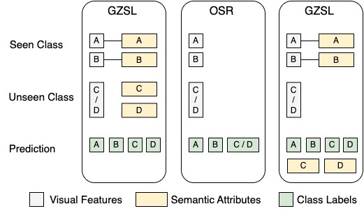
Figure 1: Schematic illustrations of GZSL, OSR, and our explored Zero-Knowledge Zero-Shot Learning (ZK-ZSL).

We propose a novel framework to tackle the ZK-ZSL problem and address the above challenges. In what follows, we first discuss how our proposed method takes into account the aforementioned challenges, and then we summarize our main contributions. To recognize seen classes and discover the structures of novel categories, our method learns to cluster on the target data consisting of both seen and unseen categories. Meanwhile, the class structures of seen categories are guided by the source labels. In addition, to mitigate the unavailability problem of unseen semantic labels, we enforce a structural alignment between recovered hidden embedding and predicted semantic space to aid the semantic learning of unseen categories with their discovered clustering structures. Our main contributions can be summarized as follows:

• We formulate and explore a new visual recognition setting named Zero-Knowledge Zero-Shot Learning (ZK-ZSL) that aims to recognize seen and unseen categories without prior knowledge and recovers unseen semantic attributes, addressing the limitations of GZSL and OSR in practical use.

• We propose a novel method that learns to uncover clustering structures in the target dataset guided by labeled seen class structures. A novel structural alignment loss is designed to aid the learning of novel semantic attributes with recovered clustering structures.

• We demonstrate the superiority of our method in terms of classification and semantic recovery on four benchmark datasets by comparing with five competitive baseline methods. We also provide rich in-depth explorations of our method for unseen category discovery.

2 Related Works

Generalized Zero-Shot Learning. The demand to recognize novel classes not present during training without additional labeling motivates the area of Zero-Shot Learning (ZSL). In ZSL, class-level semantic attributes are provided to aid knowledge transfer from source to the target dataset. Later, due to the disjoint nature of the source and target label spaces, GZSL is hence proposed [28], where the target dataset consists of categories present in the source dataset and additional novel categories. Existing GZSL methods can be categorized into embedding-based and generative-based methods. Embedding-based methods learn to map visual features to the semantic space and make predictions based on the similarity between predicted semantics and ground truth [9, 1, 29, 43, 40, 41, 22]. Generative-based methods synthesize samples from semantic attributes through Generative Adversarial Networks (GANs) [11] or Variational Autoencoders (VAEs) [19], and reformulate the GZSL problem to a conventional supervised learning problem by training a classifier with generated samples [21, 38, 24, 45, 44].

Open-Set Recognition. OSR extends the traditional closed-set classification setting by assuming the target samples contain categories seen during training and additional unseen categories. Under OSR, classifiers need to be able to recognize seen samples and reject unknown samples [10]. OSR methods usually adopt a threshold-based strategy, where the threshold can be empirically chosen. Existing methods differ in how they discriminate seen categories, including SVM-based [6, 30, 31, 15], distance-based [2, 26, 23], and deep learning based methods[3, 12, 32, 14, 17].

In addition to GZSL and OSR, we notice the recently proposed Semantic Recovery Open-Set Domain Adaptation (SR-OSDA) [16] and the Generalized Category Discovery (GCD) [34, 36, 5] are related to our setting. SR-OSDA aims to recognize both seen and unseen samples in the target dataset and recover their semantic attributes. The goal of GCD is to automatically categorize a partially labeled dataset of images, where the unlabeled images contain both seen and novel categories, but GCD does not consider semantic recovery.

3 Motivation and Problem Definition

GZSL aims to recognize categories both seen and unseen during training, given semantic attributes of all classes. However, novel categories are pre-defined with semantic labels and are known to the model, which can be impractical for some applications. OSR aims to detect unseen samples without prior information but treats them as one group, failing to explore their innate structures further. Moreover, the semantic attributes of visual categories are not utilized under OSR, which prevents in-depth analyses and interpretations of the structures of novel categories.

Due to the limitations of GZSL and OSR, we consider the Zero-Knowledge Zero-Shot Learning (ZK-ZSL) problem, which focuses on recognizing seen and unseen categories without prior knowledge of novel semantic labels while uncovering the partitional structures of novel categories and their missing semantic attributes. Inspired by the paradigm style in Pourpanah et al. [28], we illustrate the main differences among GZSL, OSR, and ZK-ZSL in Figure 1. Compared with GZSL and OSR, ZK-ZSL is more realistic in that it does not assume prior knowledge of the unseen categories, and it can support richer analysis and interpretation of the discovered novel categories. Here we provide problem formulation of ZK-ZSL: Let $D_{s}=\{X_{s},Y_{s},A_{s}\}$ be the source dataset, and $D_{t}=\{X_{t}\}$ be the target dataset. Given both $D_{s}$ and $D_{t}$, ZK-ZSL aims to find $X_{t}$’s corresponding $Y_{t}$, which contains all visual categories in $Y_{s}$ and some additional unseen categories $Y_{u}=Y_{t}\setminus Y_{s}$, and recover their semantic attributes $A_{t}$. Table 1 summarizes the major notations used in this paper.

Table 1: Notions and descriptions

Notion	Type	Description
$X_{s}/X_{t}$	Input	source/target visual features
$A_{s}/A_{t}$	Input	source/target semantic attributes
$Y_{s}/Y_{t}$	Input	source/target labels
$K_{s}/K_{t}$	Input	source/target number of categories
$N_{s}/N_{t}$	Input	source/target number of instances
$d$	Input	dimension of semantic attribute
$z_{s}/z_{t}$	Learnable	source/target embedding
$\hat{a}_{s}/\hat{a}_{t}$	Learnable	source/target predicted semantic
$\tilde{\mu}_{k}$	Learnable	seen class prototype by pseudo label
$\mu_{k}$	Learnable	class prototype

The challenges associated with ZK-ZSL are twofold. First, the model needs to provide partitional structures of unseen categories. However, training a visual classifier only with labeled seen samples can only help distinguish between seen/unseen categories but cannot further separate the fine-grained categories in the unseen class. In addition, due to mismatched label spaces in the source and target dataset, learning such a classifier could destroy the clustering structures of novel categories. Second, since the semantic attributes of unseen categories are unavailable, learning only with seen semantics is prone to overfitting and results in biased semantic prediction.

4 Proposed Method

In this section, we introduce our framework for ZK-ZSL and the objective function to train our framework.

4.1 Framework Overview

Figure 2 shows our proposed framework for ZK-ZSL. In order to discover and differentiate novel categories while recognizing seen classes, our method learns to recover the clustering structures of both seen and unseen categories in the target dataset, where the learning of seen class structures is guided by the source labels. In addition, to mitigate the overfitting brought about by the unavailability of unseen semantic labels, we apply a structural alignment loss to support semantic learning with the recovered structures of unseen categories. Therefore, our framework consists of three main components for source-guided clustering, semantic prediction, and structural alignment. The source-guided clustering component learns to recover the clustering structures of both seen and unseen categories on a hidden embedding space where the learning of seen class structures is supported by labeled source data. The semantic prediction component maps the hidden embedding to the semantic space. The structural alignment component guides the semantic learning of novel categories with their recovered clustering structures.

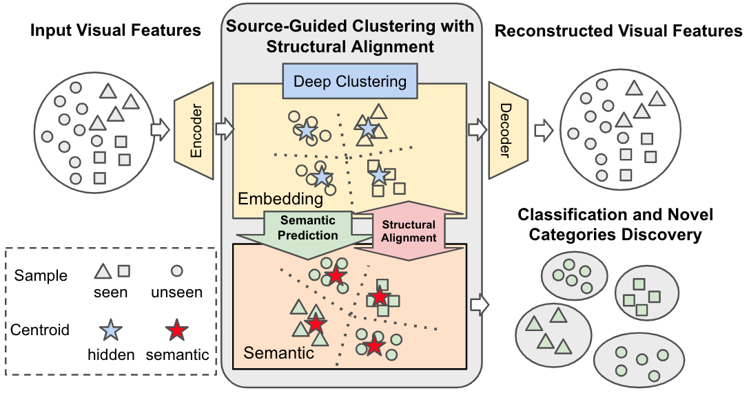
Figure 2: Overview of our proposed framework. The deep clustering component guided by the source class structures uncovers the clustering structures of the target dataset. The semantic prediction component maps the embedding space to the semantic space. The structural alignment component supports semantic learning of unseen categories with recovered structures.

4.2 Objective Function

Our learning objective consists of three main components: source-guided clustering loss, semantic prediction loss, and structural alignment loss. We denote our encoder, decoder, and semantic predictor as $g:x\rightarrow z$, $h:z\rightarrow x$, and $f:z\rightarrow a$, where $x$, $z$, and $a$ represent visual feature, hidden embedding, and semantic attribute spaces, respectively, and we define learnable cluster centroids as $\mathcal{C}=\{\mu_{1},...,\mu_{K_{t}}\}$.

Source-guided Clustering Loss. Our method learns to recover clustering structures of both seen and unseen categories guided by source labels. To achieve this, we utilize an auto-encoder to extract hidden embeddings, apply clustering regularization on the embedding space to separate both seen and unseen categories, and align seen cluster centroids with source labels. In this way, we break down the source-guided clustering loss into three parts: self-reconstruction, clustering regularization, and source centroid alignment.

Self-reconstruction. Self-reconstruction loss helps the encoder and decoder extract clustering-favorable hidden embeddings with minimal information loss. It is defined as:

$$\mathcal{L}_{self}=\frac{1}{N_{s}}\sum_{i}^{N_{s}}\lVert x^{s}_{i}-h\circ g(x^{s}_{i})\rVert^{2}_{2}+\frac{1}{N_{t}}\sum_{i}^{N_{t}}\lVert x^{t}_{i}-h\circ g(x^{t}_{i})\rVert^{2}_{2},$$ (1)

where $\circ$ represents function composition.

Clustering Regularization. Following Deep Embedding Clustering [42], we model the cluster assignment with a probability distribution. Specifically, the similarity between an embedding instance $z_{i}$ to a cluster centroid $\mu_{k}$ is measured with a Student-t distribution:

$$p^{z}_{ik}=\frac{(1+\lVert z_{i}-{\mu}_{k}\rVert^{2}_{2})^{-1}}{\sum_{j=1}^{K_{t}}(1+\lVert z_{i}-{\mu}_{j}\rVert^{2}_{2})^{-1}}.$$ (2)

Subsequently, an auxiliary target distribution is employed to strengthen cluster prediction. The target distribution is defined by

$$q^{z}_{ik}=\frac{(p^{z}_{ik})^{2}/\sum_{j}^{N_{t}}p^{z}_{jk}}{\sum_{j^{\prime}}^{K_{t}}(p^{z}_{ij^{\prime}})^{2}/\sum_{j}^{N_{t}}p^{z}_{jj^{\prime}}}.$$ (3)

The clustering regularization loss measures the difference between the cluster assignment distribution and target distribution. By minimizing their divergence, data points are pulled toward the likely cluster centroid and pushed away from others. Mathematically, the clustering regularization loss is defined as

$$\mathcal{L}_{reg}=\frac{1}{N_{t}}\sum_{i=1}^{N_{t}}D_{KL}(p^{z}_{i}||q^{z}_{i})=\frac{1}{N_{t}}\sum_{i=1}^{N_{t}}\sum_{k=1}^{K_{t}}p^{z}_{ik}\log\frac{p^{z}_{ik}}{q^{z}_{ik}}.$$ (4)

Source Centroid Alignment. The source centroid alignment loss pulls source samples toward their corresponding cluster centroids. This is achieved by optimizing the prototypical probability distribution defined by the distance between data points and cluster centroids. The prototypical probability of a data point $z_{i}$ given a cluster centroid $\mu_{k}$ is

$$\mathcal{P}(z_{i}|\mu_{k})=\frac{\exp(-d(z_{i},\mu_{k}))}{\sum_{k^{\prime}\leq K_{s}}\exp(-d(z_{i},\mu_{k^{\prime}}))},$$ (5)

where $d$ is an Euclidean distance function and the source centroid alignment loss is

$$\mathcal{L}_{cent}=\frac{1}{N_{s}}\sum_{i=1}^{N_{s}}\mathcal{L}(\mathcal{P}_{i},y_{i}),$$ (6)

where $\mathcal{L}$ denotes the cross entropy loss. To address the potential distribution drift of seen categories between the source and target dataset, we incorporate an optional loss to reduce the gap between source and target seen class centroids. We first define the expected target seen class centroid

$$\tilde{\mu}_{k}:=\mathbb{E}_{\hat{y}^{t}_{i}=k}z^{t}_{i},$$ (7)

where $\hat{y}^{t}_{i}=\arg_{k}\max p^{z}_{ik}$ is the pseudo label obtained from cluster assignment probability. The source centroid alignment loss under distribution shift is defined as

$$\mathcal{L}_{cent}=\frac{1}{N_{s}}\sum_{i=1}^{N_{s}}\mathcal{L}(\mathcal{P}_{i},y^{i}_{s})+\frac{1}{K_{s}}\sum_{k=1}^{K_{s}}\lVert\tilde{\mu}_{k}-\mu_{k}\rVert^{2}_{2}.$$ (8)

Finally, the source-guided clustering loss combines self-reconstruction loss, clustering regularization loss, and source centroid alignment loss:

$$\mathcal{L}_{c}=\mathcal{L}_{self}+\mathcal{L}_{reg}+\mathcal{L}_{cent}.$$ (9)

Semantic Prediction Loss. Following Frome et al. [9], we use a pairwise ranking loss to learn the embedding-to-semantic mapping, where we stop penalizing false terms after the maximum margin of 0.5 is reached.

$$\mathcal{L}_{a}=\frac{1}{N_{s}}\sum_{i=1}^{N_{s}}\sum_{k\neq y_{s}^{i}}\max\{0,0.5-A_{y_{i}}^{\top}a^{s}_{i}+A_{k}^{\top}a^{s}_{i}\},$$ (10)

where $A_{k}$ is the ground truth semantic label of class $k$.

Structural Alignment Loss. Structural alignment guides semantic learning by transferring the structural knowledge in the embedding space to the semantic space. Specifically, the structural alignment loss minimizes the divergence between embedding and semantic cluster structures modeled by the cluster assignment probability. We have defined the cluster assignment probability in the embedding space $p_{ik}^{z}$ in Eq. (2). Similarly, the cluster assignment probability in the semantic space can be defined by $p^{a}_{ik}$, where

$$p^{a}_{ik}=\frac{(1+\lVert a_{i}-f(\mu_{k})\rVert^{2}_{2})^{-1}}{\sum_{j=1}^{K_{t}}(1+\lVert a_{i}-f(\mu_{j})\rVert^{2}_{2})^{-1}}.$$ (11)

Based on Eq. (2) and Eq. (11), we define the structural alignment loss as

$$\mathcal{L}_{align}=\frac{1}{N_{t}}\sum_{i=1}^{N_{t}}\sum_{j=1}^{N_{t}}({p_{i}^{z}}^{\top}p_{j}^{z}-{p_{i}^{a}}^{\top}p_{j}^{a})^{2},$$ (12)

where ${p_{i}^{z}}^{\top}p_{j}^{z}$ measures the probability that data points $i$ and $j$ in the embedding space belonging to the same cluster.

Overall Objective Function. The overall learning objective is to minimize the source-guided clustering loss, semantic prediction loss, and structural alignment loss:

$$\min_{g,h,f,\mathcal{C}}\mathcal{L}_{c}+\alpha\mathcal{L}_{a}+\beta\mathcal{L}_{align},$$ (13)

where $\alpha$ and $\beta$ are trade-off parameters.

5 Experiments

5.1 Experimental Settings

Table 2: Characteristics of four benchmark datasets.

Dataset	Source	Target_s	Target_t	$K_{s}$	$K_{t}$	$d$
APY	5932	7924	1483	20	32	64
CUB	8855	2973	1764	150	200	312
AWA2	19832	5685	4958	40	50	85
SUN	12900	1440	2580	645	717	102

• Note: Target_s and Target_t denote the sample numbers of seen and unseen categories in the target domain.

Datasets. We choose four commonly used attribute datasets: Attribute Pascal and Yahoo (APY) [8], Animals with Attributes 2 (AWA2) [20], Caltech-UCSD-Birds 200-2011 (CUB) [35], and SUN dataset [39]. We split the data into the source and target sets by following the split strategy in Xian et al. [37]. All visual features are obtained from ResNet-101 [13] pre-trained on ImageNet [7]. Table 2 summarizes the key characteristics of these datasets. Only the semantic attributes of seen categories are available for training. We use unit vectors as semantic representations.

Competitive Methods. We compare our method with established methods in Generalized Zero-Shot Learning and Semantic Recovery Open-Set Domain Adaptation. For GZSL based methods, it is noteworthy that not all established methods work under our setting, where unseen semantics are not provided. For example, generative-based methods, which require unseen semantics to synthesize samples of novel categories, are not applicable under ZK-ZSL. We compare with DEVISE [9], ESZSL [29], SJE [1] and SDGZSL [4]. In particular, DEVISE, SJE, and ESZSL aim to find a mapping from visual space to semantic space, while SDGZSL learns a hidden embedding from visual features that can be decomposed to semantic-consistent representation and semantic-unrelated representation. In the next section, we elaborate on how to tailor the above methods to the ZK-ZSL setting. In addition, we compare with Jing et al. [16] as the only existing SR-OSDA-based method. Their approach progressively separates seen and unseen samples with pseudo labels obtained from prototypical probabilities and utilizes a graph neural network for semantic attribute prediction to avoid overfitting.

Implementation. Here we first introduce how we extend the competitive methods for novel category prediction, then elaborate on the implementation details of our method.

Since the competitive methods only predict semantic attributes or hidden embeddings, we need to extend their approaches to support novel categories prediction. To this end, we adopt a two-step procedure that first recognizes seen and unseen samples and then further separates unseen samples with K-means. We rely on the prototypical probability defined in Eq. (5) for seen/unseen separation. We first define the highest prototypical probability that a data point belongs to a seen category:

$$\mathcal{P}^{max}_{i}=\max_{k}\mathcal{P}(z_{t}^{i}|\mu_{k}).$$ (14)

Data points with higher $\mathcal{P}^{max}$ are more likely from a seen category, while unseen samples tend to have more even prototypical probability distributions, and thus lower $\mathcal{P}^{max}$. We follow Jing et al. [16] to choose a threshold where the data points with $\mathcal{P}^{max}$ higher than $\tau=\frac{1}{N_{t}}\sum_{i}\mathcal{P}^{max}_{i}$ are recognized as seen samples, and classified by their corresponding class centroids; those with lower $\mathcal{P}^{max}$ are regarded as unseen samples and predicted by K-means implemented by Scikit-learn [27]. Let unseen class centroids predicted by K-means be $\{\hat{\mu}_{K_{s}+1},...,\hat{\mu}_{K_{t}}\}$, we define classification prediction as

$$\hat{y}_{t}^{i}=\begin{cases}\arg\max_{k\leq K_{s}}\mathcal{P}(z_{t}^{i}|\mu_{k})&\text{if \ }\mathcal{P}^{max}_{i}\geq\tau\text{,}\\ \arg\min_{K_{s}<k\leq K_{t}}d(z_{t}^{i},\hat{\mu}_{k})&\text{otherwise.}\end{cases}$$ (15)

In our framework, the encoder and decoder constitute a de-noising autoencoder. Specifically, the encoder and decoder are 5 linear layers followed by batch normalization and Leaky ReLU activation. Their neural structures are dropout-2048-512-256-256-4096-$h$ and dropout-$h$-4096-256-256-512-2048, respectively, where $h$ is the dimension of the hidden embeddings. We set the dropout rate to $0.01$ for all experiments and choose $h=256$ for APY and AWA2 datasets and $h=1024$ for CUB and SUN datasets. The semantic prediction head is a linear layer with batch normalization. Our model parameters are initialized by pretraining with self-reconstruction loss and semantic prediction loss, and class centers are initialized with K-means. We use Adam optimizer [18] with a learning rate of $1e^{-3}$ and weight decay of $1e^{-5}$ in the pretraining stage, and then learning rate is adjusted to $1e^{-4}$ for training. Learning rates are reduced by a factor of 0.1 every 200 epochs for both stages.

Metrics. We evaluate model performance from two perspectives: classification and semantic recovery accuracy.

Table 3: Classification and Semantic Recovery Accuracy on four benchmark datasets.

	Dataset	APY			CUB			AWA2			SUN
	Method	$Acc_{s}$	$Acc_{u}$	$Acc_{h}$	$Acc_{s}$	$Acc_{u}$	$Acc_{h}$	$Acc_{s}$	$Acc_{u}$	$Acc_{h}$	$Acc_{s}$	$Acc_{u}$	$Acc_{h}$
Classification	DEVISE∗	$76.4$	$13.0$	$22.2$	$37.1$	$15.8$	$22.2$	$69.2$	$24.5$	$36.2$	$18.4$	$21.9$	$20.0$
	ESZSL∗	$77.2$	$17.0$	$27.8$	$35.9$	$23.8$	$28.6$	$67.5$	$40.3$	$50.4$	$16.6$	$18.6$	$17.6$
	SJE∗	$74.1$	$9.2$	$16.3$	$34.1$	$9.3$	$14.6$	$57.0$	$13.2$	$21.5$	$17.2$	$17.6$	$17.4$
	SDGZSL⋄	$71.1$	$22.5$	$34.2$	$58.0$	$33.6$	$42.5$	$79.6$	$27.9$	$41.4$	$32.8$	$26.5$	$29.3$
	SR-OSDA∗	$24.2$	$15.4$	$18.8$	$2.7$	$11.7$	$4.4$	$27.0$	$18.6$	$22.0$	$5.0$	$11.7$	$9.7$
	Ours	$48.2$	$30.6$	$37.4$	$43.8$	$35.4$	$39.2$	$82.8$	$47.6$	$60.5$	$23.5$	$24.8$	$24.1$
	Method	$SR_{s}$	$SR_{u}$	$SR_{h}$	$SR_{s}$	$SR_{u}$	$SR_{h}$	$SR_{s}$	$SR_{u}$	$SR_{h}$	$SR_{s}$	$SR_{u}$	$SR_{h}$
Semantic Recovery	DEVISE	$2.6$	$9.7$	$4.1$	$37.8$	$24.4$	$29.6$	$61.1$	$26.7$	$37.2$	$29.4$	$14.8$	$19.7$
	ESZSL	$83.6$	$1.4$	$2.8$	$55.5$	$11.5$	$19.0$	$88.5$	$2.2$	$4.3$	$27.3$	$13.1$	$17.7$
	SJE	$7.5$	$9.4$	$8.3$	$0.8$	$11.6$	$1.4$	$41.8$	$20.4$	$27.4$	$27.0$	$16.8$	$20.7$
	SR-OSDA	$3.4$	$0.7$	$1.2$	$0.3$	$0.2$	$0.3$	$2.7$	$0.4$	$0.7$	$0.2$	$0.3$	$0.2$
	Ours	$60.4$	$17.5$	$27.2$	$52.4$	$25.1$	$33.9$	$84.6$	$32.9$	$47.4$	$36.8$	$18.2$	$24.4$

• Note: $*$ represents evaluation in semantic space, and $\diamond$ represents evaluation in embedding space.

In the same spirit of the evaluation metrics proposed in Xian et al. [37], our classification accuracy measures the class average accuracy of seen and unseen categories and their harmonic mean. We define the classification accuracy of seen categories as the average per-class accuracy:

$$Acc_{s}=\frac{1}{N_{s}}\sum_{k\leq K_{s}}\frac{\sum_{i}\mathds{1}_{\hat{y}_{t}^{i}=y_{t}^{i}}}{\sum_{i}\mathds{1}_{y_{t}^{i}=k}},$$ (16)

where $\mathds{1}$ is an indicator function. Similarly, we define the classification accuracy of unseen category as

$$Acc_{u}=\frac{1}{N_{t}-N_{s}}\sum_{K_{s}<k\leq K_{t}}\frac{\sum_{i}\mathds{1}_{map(\hat{y}_{t}^{i})=y_{t}^{i}}}{\sum_{i}\mathds{1}_{y_{t}^{i}=k}},$$ (17)

where $map()$ is a permutation function that maps predicted unseen categories to ground-truth unseen counterparts. Finally, we evaluate the harmonic mean of seen and unseen classification accuracy:

$$Acc_{h}=2\times\frac{Acc_{s}\times Acc_{u}}{Acc_{s}+Acc_{u}}.$$ (18)

;

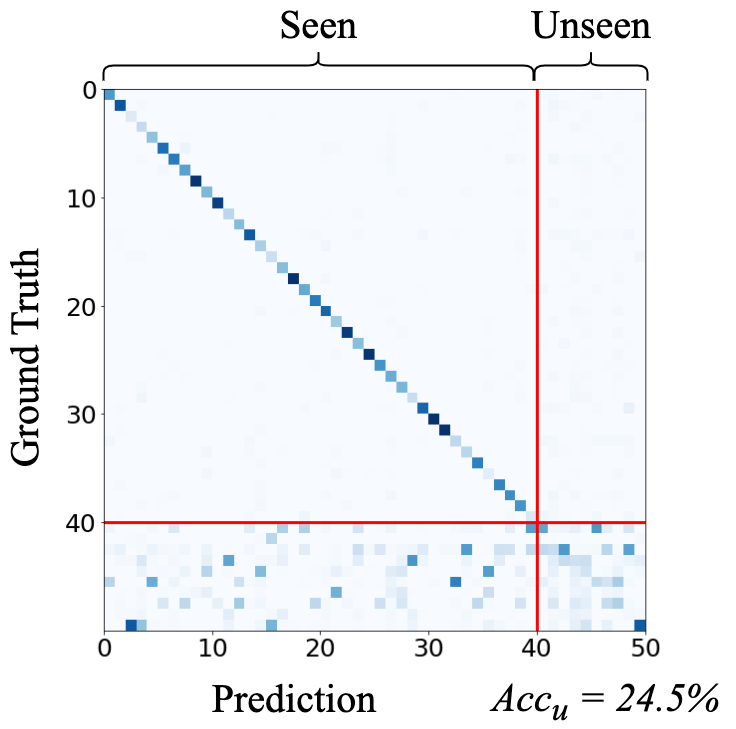
(a) DEVISE

;

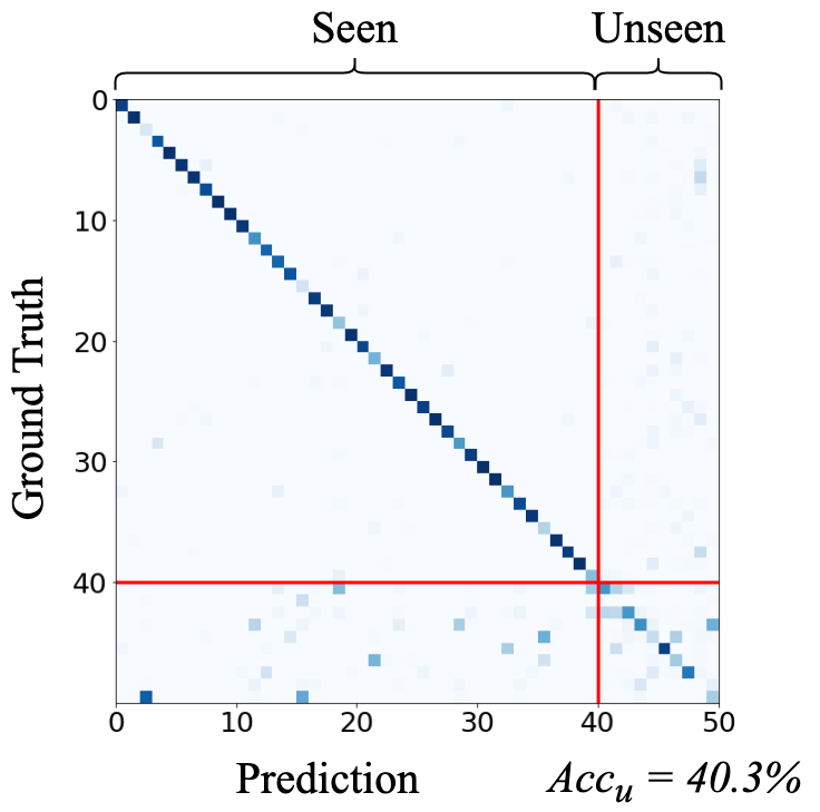
(b) ESZSL

;

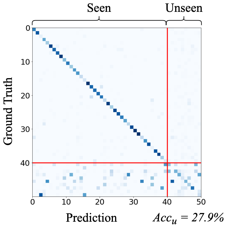
(c) SDGZSL

;

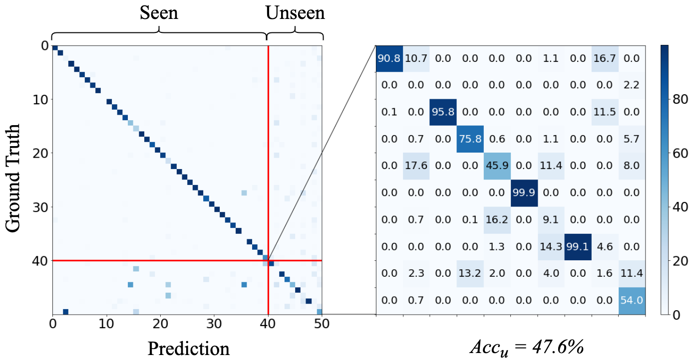
(d) Ours

Figure 3: Confusion matrices of seen and unseen categories on the AWA2 dataset. Recommended to zoom in for better visualization.

In addition to classification accuracy, we want to evaluate the model’s ability to accurately uncover the target dataset’s semantic attributes. Following Xian et al. [37], we define the semantic recovery prediction as

$$\tilde{y}_{t}^{i}=\arg\max_{k}A_{k}^{\top}a_{t}^{i}.$$ (19)

Similarly, semantic recovery accuracies $SR_{s}$, $SR_{u}$, and $SR_{h}$ follow the derivation of classification accuracies.

For DEVISE, SJE, and ESZSL, we evaluate their classification accuracies with their predicted semantic attributes, where the class centroids of seen categories are ground truth semantic labels. We evaluate SDGZSL classification ability with its generated semantic-consistent representation, and because it does not have a semantic prediction component, we exclude it from semantic recovery evaluation. We use the cosine distance when calculating prototypical probability in the semantic space and use Euclidean distance in the embedding space.

5.2 Performance

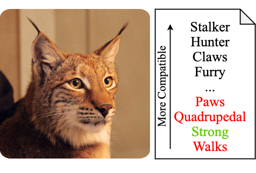
(a) Bobcat

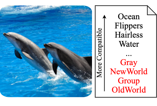
(b) Dolphin

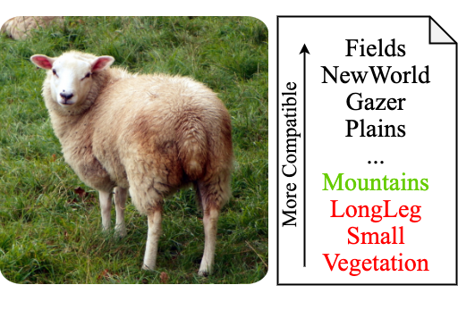
(c) Sheep

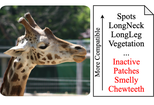
(d) Giraffe

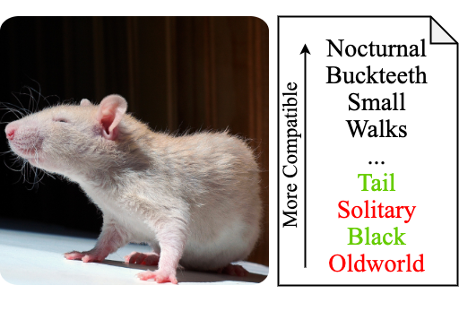
(e) Rat

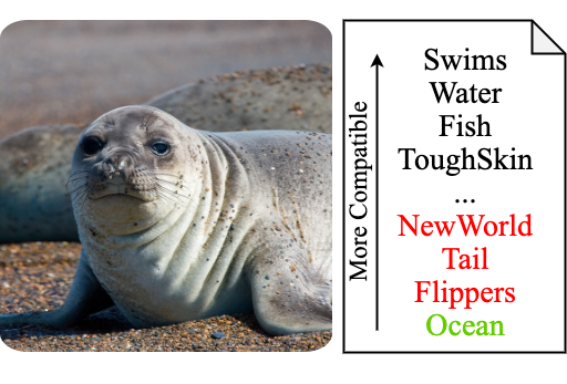
(f) Seal

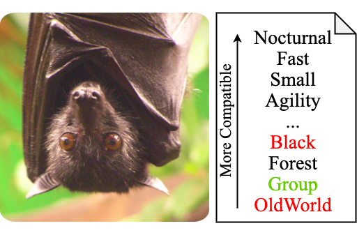
(g) Bat

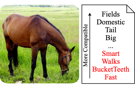
(h) Horse

Figure 4: Examples of novel categories and predicted semantic attributes. The predicted semantics are ordered by compatibility with ground-truth labels, where the top is the most compatible semantic attribute. Red indicates a wrong prediction, and Green indicates a wrong prediction but is consistent with the given instance.

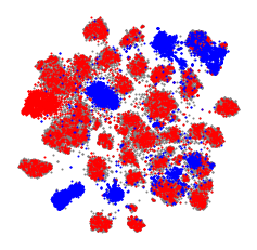
(a) ResNet

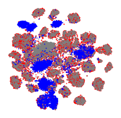
(b) SJE

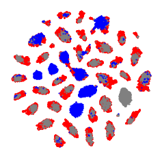
(c) Ours (embedding)

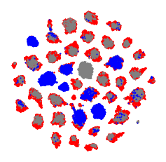
(d) Ours (semantic)

Figure 5: t-SNE visualization of (a) ResNet features, (b) semantic attribute predicted by SJE [1], (c) hidden embedding generated by our method, and (d) semantic attribute predicted by our method. Red represents source data points. Blue and Gray highlight data points in the target dataset that belong to unseen and seen categories, respectively.

Table 3 summarizes the classification accuracy and semantic recovery accuracy for four benchmark datasets, where red and blue highlight the highest and second highest accuracies.

For the classification accuracy measurement, we obverse that our method attains the best overall performance in APY and AWA2 while achieving the second-highest overall accuracy in CUB and SUN. It is noteworthy that for the AWA2 dataset, our method brings a 10.1% overall accuracy improvement compared with the second-highest baseline. Our superior performance in APY and AWA2 partly results from our improved unseen category classification accuracy, which demonstrates the effectiveness of our structural alignment and source-guided clustering component. In comparison, we see a trend of overfitting on the source dataset for some baseline methods, which destroys the clustering structure of unseen samples. For example, regarding the performance on the APY dataset, DEVISE achieves 76.4% seen classification accuracy but only attains 13.0% for the unseen category. In addition, we observe our method does not improve overall classification accuracy in CUB and SUN, compared with the best-performing SDGZSL baseline. We hypothesize that this is due to a reduced number of samples per class in the target dataset. There are, on average, 293 and 212 samples per class in APY and AWA2, respectively, but for CUB and SUN there are only 23 and 6 samples. This leads to (1) distribution drift of seen category samples, which undermines our method’s capability to classify seen samples correctly, and (2) underrepresented novel class samples, which complicates their clustering structures recovery.

For the semantic recovery accuracy measurement, our method achieves the best performance in terms of unseen category semantic recovery and overall semantic recovery accuracy. This demonstrates that our structural alignment loss can effectively prevent overfitting on the source semantic data and accurately predict the semantic attributes of unseen categories. In comparison, we observe a similar pattern in classification that some baselines can accurately recover semantics of seen categories, but not for unseen samples. For example, ESZSL achieves 83.6% for seen semantic recovery but only 1.4% for unseen categories.

5.3 Factor Exploration

To further explore our method, we explore confusion matrices of seen and unseen categories, visualize representations obtained by our method, showcase some representative samples and their associated predictions, analyze the ablation study of our model components, and visualize our predicted semantic attributes of novel categories with word clouds. Finally, we explore hyper-parameters $\alpha$ and $\beta$.

Confusion Matrices. We visualize confusion matrices of different methods on the AWA2 dataset, including DEVISE, ESZSL, SDGZSL, and ours in Figure 3. We observe that our method has much fewer false predictions for novel categories. It is noteworthy that our method classifies four unseen categories with 90+% accuracy. We also see that our method improves classification accuracy for seen categories.

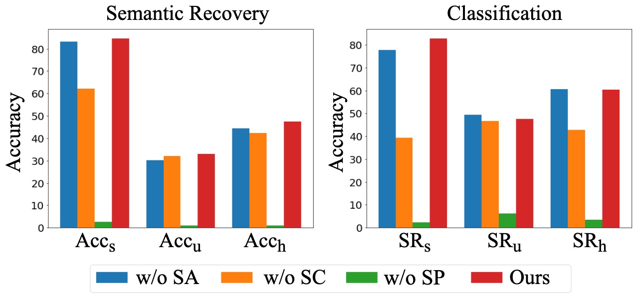
Figure 6: Ablation study results of our proposed method on AWA2 dataset. We report the performance of variants that are trained without structural alignment loss (SA), without source-guided clustering loss (SC), without semantic prediction loss (SP), and with our proposed method. The left shows semantic recovery accuracy, and the right shows classification accuracy.

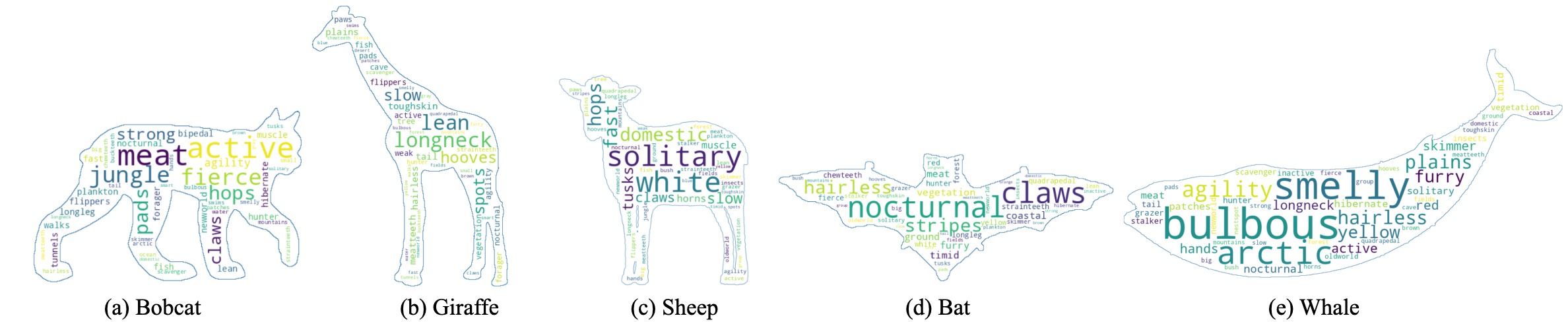
Figure 7: Word clouds of novel category semantics predicted by our model, including (a) bobcat, (b) giraffe, (c) sheep, (d) bat, and (e) whale. Recommended to zoom in for better visualization.

Representation Visualization. In Figure 5, we visualize different representations of the AWA2 dataset with t-SNE [33], including the ResNet features, semantic attributes predicted by SJE, our method’s hidden embedding, and our predicted semantic attributes. Red dots represent data points in the source dataset, while blue and gray dots represent target data points that belong to seen and unseen categories, respectively. For our hidden embedding visualization, we observe a much clearer separation among clusters compared with the ResNet input and SJE prediction, which is achieved with our source-guided clustering component. In addition, our recovered semantic attributes have similar structures of hidden embeddings, showing that our structural alignment loss is effective.

Qualitative Analysis. In Figure 4, we showcase some representative samples from novel categories in the AWA2 dataset, including the input image and predicted semantic attributes ordered by compatibility to the ground-truth semantic labels. The compatibility is calculated by an element-wise multiplication between the predicted semantic attribute scores and ground truth. We regard a predicted attribute with positive compatibility as a correct prediction and vice versa. The most compatible predicted semantics are discriminative for the given category. For least compatible attributes, some valid attributes are not predicted, which is indicated by red in Figure 4, and some predicted attributes (in green) are not relevant to the given category but reasonable for the given instance.

Ablation Study. We explore the effectiveness of our designed components with an ablation study. Specifically, we individually train variants of our framework with the AWA2 dataset that are (1) without structural alignment loss $\mathcal{L}_{align}$, (2) without source-guided clustering loss $\mathcal{L}_{c}$, and (3) without semantic prediction loss $\mathcal{L}_{a}$. In Figure 6, we report and compare the classification accuracy and semantic recovery accuracy. We first observe that our method achieves the best overall performance when trained with all objectives. In addition, semantic recovery accuracy and seen category classification accuracy are improved with structural alignment loss, which indicates that structural alignment helps hidden embedding and semantic learning.

Novel Category Visualization. Figure 7 visualizes our predicted semantic attributes of discovered novel categories through word clouds generated by Mueller [25]. We select the 50 most significant attributes ordered by their predicted scores for visualization and adjust font sizes according to their relative ranking. We observe that the most significant attributes are consistent with the corresponding category.

Hyperparameter Analysis. $\alpha$ and $\beta$ control the contributions of the semantic prediction loss and structural alignment loss and, by default, are set to 1.0 and 1.0. Here we explore the volatility of these parameters and verify our default choice by doing a hyperparameter analysis on the AWA2 dataset. When $\alpha$ is fixed at 1.0, and $\beta$ is explored in the range of $\{0,0.1,0.5,1.0,5.0,10.0\}$, we observe that the classification and semantic recovery accuracy increase as $\beta$ increases, and reach the optimal values of $59.7\%$ and $50.9\%$ when $\alpha=1.0$ and $\beta=1.0$. As $\beta$ further increases, $Acc_{u}$ and $SR_{u}$ decline to $30.6\%$ and $45.4\%$. When $\beta$ is pinned at 1.0 and $\alpha$ is set in the range of $\{0,0.1,0.5,1.0,5.0,10.0\}$, the $Acc_{u}$ and $SR_{u}$ form an inverted U pattern where they start at $47.0\%$ and $0.3\%$, reach the optimal combination, then reduce to $56.8\%$ and $42.1\%$. The optimal values are obtained at $\alpha=\beta=1.0$.

6 Conclusion

In this work, we explore a novel and practical setting in visual recognition named Zero-Knowledge Zero-Shot Learning, addressing the limitations of GZSL and OSR. ZK-ZSL aims to recognize categories present in the source dataset as well as additional novel categories without prior knowledge and recover their semantic attributes. We consider the challenges associated with ZK-ZSL from two aspects: (1) the demand to further separate unseen categories, where training a classifier with only source labels could destroy the structures of unseen categories, and (2) the unavailability of unseen semantic labels that could cause inaccurate and biased semantic predictions. Our proposed method learns to recover the clustering structures of both seen and unseen categories in the target dataset, where the seen class centroids are guided by source labels. A novel structural alignment loss is designed to aid semantic learning of unseen categories with their recovered clustering structures. Experimental analyses show that our method achieves superior performance in terms of classification and semantic recovery on four benchmark datasets.

References

- Akata et al. [2015] Zeynep Akata, Scott Reed, Daniel Walter, Honglak Lee, and Bernt Schiele. Evaluation of output embeddings for fine-grained image classification. In Proceedings of the IEEE/CVF Conference on Computer Vision and Pattern Recognition, 2015.
- Bendale and Boult [2015] Abhijit Bendale and Terrance Boult. Towards open world recognition. In Proceedings of the IEEE/CVF Conference on Computer Vision and Pattern Recognition, 2015.
- Bendale and Boult [2016] Abhijit Bendale and Terrance E Boult. Towards open set deep networks. In Proceedings of the IEEE/CVF Conference on Computer Vision and Pattern Recognition, 2016.
- Chen et al. [2021] Zhi Chen, Yadan Luo, Ruihong Qiu, Sen Wang, Zi Huang, Jingjing Li, and Zheng Zhang. Semantics disentangling for generalized zero-shot learning. In Proceedings of the IEEE/CVF International Conference on Computer Vision, 2021.
- Chiaroni et al. [2022] Florent Chiaroni, Jose Dolz, Ziko Imtiaz Masud, Amar Mitiche, and Ismail Ben Ayed. Mutual information-based generalized category discovery. arXiv preprint arXiv:2212.00334, 2022.
- Cortes and Vapnik [1995] Corinna Cortes and Vladimir Vapnik. Support-vector networks. Machine Learning, 20(3), 1995.
- Deng et al. [2009] Jia Deng, Wei Dong, Richard Socher, Li-Jia Li, Kai Li, and Li Fei-Fei. Imagenet: A large-scale hierarchical image database. In Proceedings of the IEEE/CVF Conference on Computer Vision and Pattern Recognition, 2009.
- Farhadi et al. [2009] Ali Farhadi, Ian Endres, Derek Hoiem, and David Forsyth. Describing objects by their attributes. In Proceedings of the IEEE/CVF Conference on Computer Vision and Pattern Recognition, 2009.
- Frome et al. [2013] Andrea Frome, Greg S Corrado, Jon Shlens, Samy Bengio, Jeff Dean, Marc’Aurelio Ranzato, and Tomas Mikolov. Devise: A deep visual-semantic embedding model. In Advances in Neural Information Processing Systems, 2013.
- Geng et al. [2020] Chuanxing Geng, Sheng-jun Huang, and Songcan Chen. Recent advances in open set recognition: A survey. IEEE Transactions on Pattern Analysis and Machine Intelligence, 43(10), 2020.
- Goodfellow et al. [2020] Ian Goodfellow, Jean Pouget-Abadie, Mehdi Mirza, Bing Xu, David Warde-Farley, Sherjil Ozair, Aaron Courville, and Yoshua Bengio. Generative adversarial networks. Communications of the ACM, 63(11), 2020.
- Hassen and Chan [2020] Mehadi Hassen and Philip K Chan. Learning a neural-network-based representation for open set recognition. In Proceedings of the SIAM International Conference on Data Mining, 2020.
- He et al. [2016] Kaiming He, Xiangyu Zhang, Shaoqing Ren, and Jian Sun. Deep residual learning for image recognition. In Proceedings of the IEEE/CVF Conference on Computer Vision and Pattern Recognition, 2016.
- Hughes et al. [2017] Mark Hughes, Irene Li, Spyros Kotoulas, and Toyotaro Suzumura. Medical text classification using convolutional neural networks. In Informatics for Health: Connected Citizen-Led Wellness and Population Health. IOS Press, 2017.
- Jain et al. [2014] Lalit P Jain, Walter J Scheirer, and Terrance E Boult. Multi-class open set recognition using probability of inclusion. In Proceedings of European Conference on Computer Vision, 2014.
- Jing et al. [2021] Taotao Jing, Hongfu Liu, and Zhengming Ding. Towards novel target discovery through open-set domain adaptation. In Proceedings of the IEEE/CVF International Conference on Computer Vision, 2021.
- Kardan and Stanley [2017] Navid Kardan and Kenneth O Stanley. Mitigating fooling with competitive overcomplete output layer neural networks. In Proceedings of International Joint Conference on Neural Networks, 2017.
- Kingma and Ba [2014] Diederik P Kingma and Jimmy Ba. Adam: A method for stochastic optimization. arXiv preprint arXiv:1412.6980, 2014.
- Kingma and Welling [2013] Diederik P Kingma and Max Welling. Auto-encoding variational bayes. arXiv preprint arXiv:1312.6114, 2013.
- Lampert et al. [2013] Christoph H Lampert, Hannes Nickisch, and Stefan Harmeling. Attribute-based classification for zero-shot visual object categorization. IEEE Transactions on Pattern Analysis and Machine Intelligence, 2013.
- Li et al. [2019] Jingjing Li, Mengmeng Jing, Ke Lu, Zhengming Ding, Lei Zhu, and Zi Huang. Leveraging the invariant side of generative zero-shot learning. In Proceedings of the IEEE/CVF Conference on Computer Vision and Pattern Recognition, 2019.
- Liu et al. [2021] Yang Liu, Lei Zhou, Xiao Bai, Yifei Huang, Lin Gu, Jun Zhou, and Tatsuya Harada. Goal-oriented gaze estimation for zero-shot learning. In Proceedings of the IEEE/CVF Conference on Computer Vision and Pattern Recognition, 2021.
- Mendes Júnior et al. [2017] Pedro R Mendes Júnior, Roberto M De Souza, Rafael de O Werneck, Bernardo V Stein, Daniel V Pazinato, Waldir R de Almeida, Otávio AB Penatti, Ricardo da S Torres, and Anderson Rocha. Nearest neighbors distance ratio open-set classifier. Machine Learning, 106(3), 2017.
- Mishra et al. [2018] Ashish Mishra, Shiva Krishna Reddy, Anurag Mittal, and Hema A Murthy. A generative model for zero shot learning using conditional variational autoencoders. In Proceedings of the IEEE/CVF Conference on Computer Vision and Pattern Recognition Workshops, 2018.
- Mueller [2020] Andreas Mueller. WordCloud for Python, 2020. URL https://amueller.github.io/word_cloud/. Python package version 1.8.1.
- Papa et al. [2009] Joao P Papa, Alexandre X Falcao, and Celso TN Suzuki. Supervised pattern classification based on optimum-path forest. International Journal of Imaging Systems and Technology, 19(2), 2009.
- Pedregosa et al. [2011] F. Pedregosa, G. Varoquaux, A. Gramfort, V. Michel, B. Thirion, O. Grisel, M. Blondel, P. Prettenhofer, R. Weiss, V. Dubourg, J. Vanderplas, A. Passos, D. Cournapeau, M. Brucher, M. Perrot, and E. Duchesnay. Scikit-learn: Machine learning in Python. Journal of Machine Learning Research, 12, 2011.
- Pourpanah et al. [2022] Farhad Pourpanah, Moloud Abdar, Yuxuan Luo, Xinlei Zhou, Ran Wang, Chee Peng Lim, Xi-Zhao Wang, and QM Jonathan Wu. A review of generalized zero-shot learning methods. IEEE Transactions on Pattern Analysis and Machine Intelligence, 2022.
- Romera-Paredes and Torr [2015] Bernardino Romera-Paredes and Philip Torr. An embarrassingly simple approach to zero-shot learning. In Proceedings of International Conference on Machine Learning, 2015.
- Scheirer et al. [2012] Walter J Scheirer, Anderson de Rezende Rocha, Archana Sapkota, and Terrance E Boult. Toward open set recognition. IEEE Transactions on Pattern Analysis and Machine Intelligence, 35(7), 2012.
- Scheirer et al. [2014] Walter J Scheirer, Lalit P Jain, and Terrance E Boult. Probability models for open set recognition. IEEE Transactions on Pattern Analysis and Machine Intelligence, 36(11), 2014.
- Shu et al. [2017] Lei Shu, Hu Xu, and Bing Liu. Doc: Deep open classification of text documents. arXiv preprint arXiv:1709.08716, 2017.
- Van der Maaten and Hinton [2008] Laurens Van der Maaten and Geoffrey Hinton. Visualizing data using t-sne. Journal of Machine Learning Research, 9(11), 2008.
- Vaze et al. [2022] Sagar Vaze, Kai Han, Andrea Vedaldi, and Andrew Zisserman. Generalized category discovery. In Proceedings of the IEEE/CVF Conference on Computer Vision and Pattern Recognition, 2022.
- Wah et al. [2011] Catherine Wah, Steve Branson, Peter Welinder, Pietro Perona, and Serge Belongie. The caltech-ucsd birds-200-2011 dataset. 2011.
- Wen et al. [2022] Xin Wen, Bingchen Zhao, and Xiaojuan Qi. A simple parametric classification baseline for generalized category discovery. arXiv preprint arXiv:2211.11727, 2022.
- Xian et al. [2017] Yongqin Xian, Bernt Schiele, and Zeynep Akata. Zero-shot learning-the good, the bad and the ugly. In Proceedings of the IEEE/CVF Conference on Computer Vision and Pattern Recognition, 2017.
- Xian et al. [2018] Yongqin Xian, Tobias Lorenz, Bernt Schiele, and Zeynep Akata. Feature generating networks for zero-shot learning. In Proceedings of the IEEE/CVF Conference on Computer Vision and Pattern Recognition, 2018.
- Xiao et al. [2010] Jianxiong Xiao, James Hays, Krista A Ehinger, Aude Oliva, and Antonio Torralba. Sun database: Large-scale scene recognition from abbey to zoo. In Proceedings of the IEEE/CVF Conference on Computer Vision and Pattern Recognition, 2010.
- Xie et al. [2019] Guo-Sen Xie, Li Liu, Xiaobo Jin, Fan Zhu, Zheng Zhang, Jie Qin, Yazhou Yao, and Ling Shao. Attentive region embedding network for zero-shot learning. In Proceedings of the IEEE/CVF Conference on Computer Vision and Pattern Recognition, 2019.
- Xie et al. [2020] Guo-Sen Xie, Li Liu, Fan Zhu, Fang Zhao, Zheng Zhang, Yazhou Yao, Jie Qin, and Ling Shao. Region graph embedding network for zero-shot learning. In Proceedings of European conference on computer vision, 2020.
- Xie et al. [2016] Junyuan Xie, Ross Girshick, and Ali Farhadi. Unsupervised deep embedding for clustering analysis. In Proceedings of International Conference on Machine Learning, 2016.
- Xu et al. [2020] Wenjia Xu, Yongqin Xian, Jiuniu Wang, Bernt Schiele, and Zeynep Akata. Attribute prototype network for zero-shot learning. In Advances in Neural Information Processing Systems, 2020.
- Yu et al. [2020] Yunlong Yu, Zhong Ji, Jungong Han, and Zhongfei Zhang. Episode-based prototype generating network for zero-shot learning. In Proceedings of the IEEE/CVF Conference on Computer Vision and Pattern Recognition, 2020.
- Zhu et al. [2018] Yizhe Zhu, Mohamed Elhoseiny, Bingchen Liu, Xi Peng, and Ahmed Elgammal. A generative adversarial approach for zero-shot learning from noisy texts. In Proceedings of the IEEE/CVF Conference on Computer Vision and Pattern Recognition, 2018.