Learning to Select Pivotal Samples for Meta Re-weighting

Abstract

Sample re-weighting strategies provide a promising mechanism to deal with imperfect training data in machine learning, such as noisily labeled or class-imbalanced data. One such strategy involves formulating a bi-level optimization problem called the meta re-weighting problem, whose goal is to optimize performance on a small set of perfect pivotal samples, called meta samples. Many approaches have been proposed to efficiently solve this problem. However, all of them assume that a perfect meta sample set is already provided while we observe that the selections of meta sample set is performance-critical. In this paper, we study how to learn to identify such a meta sample set from a large, imperfect training set, that is subsequently cleaned and used to optimize performance in the meta re-weighting setting. We propose a learning framework which reduces the meta samples selection problem to a weighted K-means clustering problem through rigorously theoretical analysis. We propose two clustering methods within our learning framework, Representation-based clustering method (RBC) and Gradient-based clustering method (GBC), for balancing performance and computational efficiency. Empirical studies demonstrate the performance advantage of our methods over various baseline methods.

Introduction

Recently, with the advent of the data-centric AI era (Miranda 2021; Polyzotis and Zaharia 2021; Hajij et al. 2021), there is an increasing concern about the quality of data for training neural network models. How to construct and maintain a high-quality data set is extremely challenging due to the existence of various defects in real-life data, e.g., imperfect labels or imbalanced distributions across classes. To tackle these issues, various techniques have been explored. One such example is the sample re-weighting strategy (Shu et al. 2019; Ren et al. 2018; Hu et al. 2019; Jiang et al. 2018; Chang, Learned-Miller, and McCallum 2017), which targets jointly learning to obtain re-weighted training samples and training neural nets upon them.

One promising strategy for learning to re-weight training samples is to leverage the framework of meta learning (Hospedales et al. 2021; Andrychowicz et al. 2016; Thrun and Pratt 2012) by formulating this problem as a bi-level optimization problem (Shu et al. 2019; Ren et al. 2018; Hu et al. 2019). In this approach, the weights of training samples are learned so that the performance of the models learned on the re-weighted training samples is maximized on a small set of perfect samples—referred to as meta samples. Existing works mainly focus on designing computationally efficient algorithms for solving this bi-level optimization problem. For example, (Shu et al. 2019) propose a meta re-weighting algorithm which alternates between updates to the model parameters and the sample weights. These algorithms, however, rely on the assumption that the meta sample set is given, and they construct this set by random sampling in their empirical studies. However, as the toy example in Figure 1 shows, randomly selected meta samples may perform worse than carefully selected ones by using our methods (62.9% vs. 87.1% on test accuracy), which we further verify in Section “Experiments”.

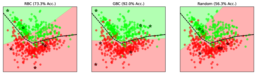
Figure 1: We produce a toy two-dimensional dataset by drawing 1000 samples from a mixture of four Gaussian distributions over two variables where the distributions are centered at the four vertices of the 2-dimensional hypercube. The upper two distributions are labeled green while the lower two are labeled red and 1% of the labels are flipped to introduce a small amount of noise to the ground truth. We visualize all the samples with their ground-truth labels in this figure. This toy dataset is then divided into 600 training, 240 testing, and 160 validation samples using a random partition, and a randomly selected 60% of the training labels are flipped. To learn a robust model (which is a neural network with two hidden layers in this example) on this noisy training set, we employ the meta-reweighting algorithm with 6 cleaned meta samples. We then show the selected meta samples (outlined with stars) and the learned decision boundaries (shaded regions) from our methods and the random selection method. The expected classifier, i.e., the learned classifier (black dotted line) on the “clean” training set is also visualized. By examining the learned classifier from these methods, we see that the one learned by random selections deviates farther from the expected classifier, thus leading to worse prediction performance than our methods (56.3% vs. 92.0%).

In this paper, we study how to learn to identify a set of meta samples from a large, imperfect training set such that the meta re-weighting performance is optimized. Specifically, we propose a framework which reduces the problem of selecting such meta samples to a weighted K-means clustering problem through rigorous theoretical analysis. This derivation basically transforms the formula for iteratively updating sample weights from the meta re-weighting algorithm into a weighted K-means clustering objective function. We can show that optimizing this objective function can aid in effectively distinguishing high-quality training samples from low-quality ones by giving them more confident sample weights (i.e. weights close to 0 or 1). This objective function, however, requires the gradients of each individual training sample as input, which is computationally expensive. To facilitate efficient evaluation of this objective function, we propose two methods, i.e. Representation-based clustering method (RBC) and Gradient-based clustering method (GBC), which balance performance with computational efficiency. Specifically, by assuming that the gradients of the bottom layers of the neural nets are insignificant, RBC only utilizes the gradient of the last layer, which is efficiently calculated through feed-forward passes. In contrast, GBC samples model parameters such that the estimation of the objective function in the above K-means problem is unbiased. Due to the necessity of explicitly (but partially) computing sample-wise gradients, GBC is slower than RBC, but can lead to better model performance in most cases.

We further explore whether our methods select reasonable meta samples for re-weighting noisily labeled data and class-imbalanced data by conducting experiments on re-weighting MNIST, CIFAR, and Imagenet-10 datasets in the presence of noisy labels or imbalanced class distribution. The results show that with the same meta re-weighting algorithm, our methods outperform other sample selection strategies in most cases.

Related Work

Sample re-weighting

The problem of re-weighting training samples for a neural network model has been extensively studied in the literature. Sample re-weighting can be beneficial for constructing robust neural network models in the presence of many defects in training data, such as corrupted labels (Han et al. 2018; Ren et al. 2018; Shu et al. 2019), biased distributions (Khan et al. 2017; Dong, Gong, and Zhu 2017), low cardinalities (Hu et al. 2019) and adversarial attacks (Holtz, Weng, and Mishne 2021). Other than solving this problem within the meta-learning framework (e.g., (Shu et al. 2019; Ren et al. 2018; Hu et al. 2019)), various strategies have been proposed for deriving sample weights. For example, in (Wang, Kucukelbir, and Blei 2017), the sample weights are modeled as a Bayesian latent variable and inferred through probabilistic models. In (Jiang et al. 2018), a mentor network is designed to derive the sample weights such that the target model does not overfit on samples with noisy labels, which falls within the curriculum learning (Bengio et al. 2009) framework. In (Kumar, Packer, and Koller 2010), the weights of training samples are determined by their training loss during the training process. However, as (Shu et al. 2019) suggests, these re-weighting techniques all perform worse than the meta re-weighting algorithm in the presence of label noise and distribution imbalance in training data.

Data efficiency

As mentioned in Section “Introduction”, it is critical to obtain large amounts of high-quality training samples for deep neural nets. However, this can be expensive and time consuming since labeling typically requires non-trivial work from human annotators, especially in scientific domains (see e.g, (Karimi et al. 2020; Irvin et al. 2019)). High labeling cost is thus a strong motivator for studies on various label efficiency techniques, e.g., active learning (see a survey in (Ren et al. 2021) and some recent works (Mirzasoleiman, Bilmes, and Leskovec 2020)), semi-supervised learning (see (Van Engelen and Hoos 2020)), and weakly-supervised learning (see Snorkel (Ratner et al. 2017)) in the past few years. All of these studies aim at minimizing human labeling effort while maintaining relatively high model performance. Note that for the meta re-weighting problem, the construction of perfect meta samples also requires human labeling effort when label noise exists. Therefore, our framework shares the same spirit as the traditional label efficiency research.

Data valuation

In the literature, other than active learning, there exists many techniques to quantify the importance of individual samples, e.g., influence function (Koh and Liang 2017) and its variants (Wu, Weimer, and Davidson 2021), Glister (Killamsetty et al. 2021), HOST-CP (Das et al. 2021), TracIn (Pruthi et al. 2020), DVRL (Yoon, Arik, and Pfister 2020) and Data Shapley value (Ghorbani and Zou 2019). However, among these methods, Data Shapley value (Ghorbani and Zou 2019) is very computationally expensive while others rely on the assumption that a set of “clean” validation samples (or meta samples) are given, which is thus not suitable for our framework (we have more detailed discussions on Data Shapley value and its extensions in Appendix “Appendix: more related work”). We therefore do not include these solutions as baseline methods.

Background: the meta re-weighting algorithm

In this section, we present some necessary details on the meta re-weighting algorithm from (Shu et al. 2019).

Suppose the meta re-weighting algorithm is conducted on a large imperfect training set, $D_{\text{train}}=\{(\textbf{x}_{j},y_{j})\}_{j=1}^{N}$ and a small perfect meta set $D_{\text{meta}}=\{(\textbf{x}_{\text{meta},i},y_{\text{meta},i})\}_{i=1}^{M}$. Imagine that we want to learn a model parameterized by $\Theta$, and the loss evaluated on a training sample $(\textbf{x}_{j},y_{j})$ and a meta sample $(\textbf{x}_{\text{meta},i},y_{\text{meta},i})$ is denoted as $f_{j}(\Theta)$ and $f_{\text{meta},i}(\Theta)$ respectively. We further denote the weight of each training sample $j$ as $w_{j}$ (between 0 and 1). Following (Shu et al. 2019), the meta re-weighting algorithm jointly learns the weights $\textbf{W}=\{w_{j}\}_{j=1}^{N}$ and the model parameter $\Theta$ by solving the following bi-level optimization problem:

$$\begin{split}&\min_{\textbf{W}}\frac{1}{M}\sum\nolimits_{i=1}^{M}f_{\text{meta},i}(\Theta^{*}(\textbf{W})),\\ &\text{s.t.}\ \Theta^{*}(\textbf{W})=\text{argmin}_{\Theta}\frac{1}{N}\sum\nolimits_{j=1}^{N}w_{j}f_{j}(\Theta),\end{split}$$ (1)

in which $\Theta^{*}(\textbf{W})$ denotes the learned model parameters on the training set weighted by W. This problem can be efficiently solved by the meta re-weighting algorithm proposed by (Shu et al. 2019), which can be abstracted with the following formulas :

Meta re-weighting:

$$\hat{\Theta}(\textbf{W}_{t})=\Theta_{t}-\frac{\alpha_{t}}{N}\sum\nolimits_{j=1}^{N}w_{j,t}\nabla_{\Theta}f_{j}(\Theta)|_{\Theta=\Theta_{t}}$$ (2)

$$w_{j,t+1}=w_{j,t}-\frac{\eta_{t}}{M}\sum\nolimits_{i=1}^{M}\nabla_{w_{j}}f_{\text{meta},i}(\hat{\Theta}(\textbf{W}_{t}))|_{\textbf{W}=\textbf{W}_{t}}$$ (3)

$$\Theta_{t+1}=\Theta_{t}-\frac{\alpha_{t}}{N}\cdot\sum\nolimits_{j=1}^{N}w_{j,t+1}\nabla_{\Theta}f_{j}(\Theta)|_{\Theta=\Theta_{t}}$$ (4)

The above formulas show how to update the model parameter and sample weights at the $t^{th}$ iteration. Among these formulas, Equation (2) tries to update the model parameter $\Theta_{t}$ given the current sample weights $\textbf{W}_{t}=[w_{1,t},w_{2,t},\dots,w_{N,t}]$, which is then employed for updating the sample weights in Equation (3). Afterwards, in Equation (4), the updated sample weights, $\textbf{W}_{t+1}$, are inserted into Equation (2) to obtain the model parameters for the next iteration, i.e., $\Theta_{t+1}$. This process is then repeated until the convergence.

Method

Unlike (Shu et al. 2019; Hu et al. 2019; Ren et al. 2018) where the meta set $D_{\text{meta}}$ is assumed to be given, our goal is to select this set from $D_{\text{train}}$. Once this meta set is selected and possibly cleaned by humans (when noisy labels exist), the meta re-weighting algorithm can be used. We hope that the resulting model performance is optimized with respect to the sample selection strategy. We observe that one critical property of such $D_{\text{meta}}$ is that it needs to produce “significant” cumulative gradient updates (rather than near-zero gradient) in Equation (3) for every training sample $j(=1,2,\dots,N)$ and every iteration $t$ in the meta re-weighting algorithm. This can thus guarantee that good training samples are efficiently up-weighted while bad training samples are efficiently down-weighted. Therefore, our goal is to maximize the magnitude of the sum of the gradient in Equation (3) evaluated for each training sample $j$, across all iterations:

$$\begin{split}&\max_{D_{\text{meta}}}\left|\sum\nolimits_{\hat{\Theta}(\textbf{W}_{t})}1/M\cdot\sum\nolimits_{i=1}^{M}\nabla_{w_{j}}f_{\text{meta},i}(\hat{\Theta}(\textbf{W}_{t}))\right|,\\ &\text{for all $j=(1,2,\dots,N)$},\end{split}$$ (5)

which we rewrite as follows according to (Shu et al. 2019) (the constant coefficients are ignored below):

$$\begin{split}&\max_{D_{\text{meta}}}\left|\sum_{\hat{\Theta}(\textbf{W}_{t}),\Theta_{t}}\sum_{i=1}^{M}\langle\nabla_{\Theta}f_{\text{meta},i}(\Theta)|_{\Theta=\hat{\Theta}(\textbf{W}_{t})},\nabla_{\Theta}f_{j}(\Theta)|_{\Theta=\Theta_{t}}\rangle\right|,\end{split}$$ (6)

which thus represents the Frobenius inner product of the gradient of the loss between the meta sample $i$ and the training sample $j$. If the above inner product is large enough, the weight of this sample will be significantly updated. Since we want to maximize the updates of the weight of each training sample, we sum up the above formula over all training samples, leading to:

$$\begin{split}&\max_{D_{\text{meta}}}\sum_{j=1}^{N}{\left|\sum_{\hat{\Theta}(\textbf{W}_{t}),\Theta_{t}}\sum_{i=1}^{M}\langle\nabla_{\Theta}f_{\text{meta},i}(\Theta)|_{\Theta=\hat{\Theta}(\textbf{W}_{t})},\nabla_{\Theta}f_{j}(\Theta)|_{\Theta=\Theta_{t}}\rangle\right|},\end{split}$$

which can be further approximated as follows by leveraging the fact that $\hat{\Theta}(\textbf{W}_{t})$, is very close to $\Theta_{t}$:

$$\begin{split}\max_{D_{\text{meta}}}\sum_{j=1}^{N}{\left|\sum_{i=1}^{M}\sum_{\Theta_{t}}{\color[rgb]{0,0,1}\langle\nabla_{\Theta}f_{\text{meta},i}(\Theta)|_{\Theta=\Theta_{t}},\nabla_{\Theta}f_{j}(\Theta)|_{\Theta=\Theta_{t}}\rangle}\right|}\end{split}$$ (7)

Equation (7) can be further rewritten as the following Meta-Sample Search Objective (MSSO):

$$\begin{split}&\text{MSSO}:=\text{Equation }\eqref{eq: our_init_objective0}=\max_{D_{\text{meta}}}\sum_{j=1}^{N}\left|\sum_{i=1}^{M}\langle G_{j},G_{\text{meta},i}\rangle\right|,\end{split}$$ (8)

in which, we define $G_{j}=\left[G_{j}^{(1)},\dots,G_{j}^{(t)},\dots\right]$ and $G_{\text{meta},i}=\left[G_{\text{meta},i}^{(1)},\dots,G_{\text{meta},i}^{(t)},\dots\right]$ as block matrices formed by concatenating the gradients, $G_{\text{meta},i}^{(t)}:=\nabla_{\Theta}f_{\text{meta},i}(\Theta)|_{\Theta=\Theta_{t}}$ and $G_{j}^{(t)}:=\nabla_{\Theta}f_{j}(\Theta)|_{\Theta=\Theta_{t}}$, from each iteration into one matrix.

Note that the meta sample set, $D_{\text{meta}}$, needs to be selected from the training set, $D_{\text{train}}$. Thus, explicitly solving MSSO is computationally intractable since there are ${N\choose M}$ possible selections of a meta set of size $M$. In what follows, we present an approximation to MSSO with rigorous guarantees, which can be effectively solved with a weighted K-means clustering algorithm.

Approximating MSSO

We show that with reasonable assumptions, solving MSSO is approximately equivalent to searching for a set of cluster centroids, $\mathcal{C}=\{C_{i}\}_{i=1}^{M}$, i.e.,:

$$\begin{split}&\text{MSSO}\approx\max_{\mathcal{C}}\sum\nolimits_{j=1}^{N}\left|\sum\nolimits_{i=1}^{M}\langle G_{j},C_{i}\rangle\right|\\ \end{split}$$

which can be approximated by solving the following $M$-clustering objective (MCO)

$$\begin{split}&\text{MSSO}\approx\text{MCO}:=\max_{\mathcal{C}}\sum\nolimits_{j=1}^{N}\sum\nolimits_{i=1}^{M}\left|\langle G_{j},C_{i}\rangle\right|,\end{split}$$ (9)

where MSSO is approximated by moving the absolute value to the inside of the sum. The approximation above can be justified by the following Theorem.

Theorem 1.

Suppose that for each sample $i$, the positive terms in the innermost sum of Equation (8) are dominant over the negative terms or vice versa, i.e.:

$$\frac{|\sum_{\langle G_{j},C_{i}\rangle>0}\langle G_{j},C_{i}\rangle|}{|\sum_{\langle G_{j},C_{i}\rangle<0}\langle G_{j},C_{i}\rangle|}>D\gg 1,$$

$$\text{or }\frac{|\sum_{\langle G_{j},C_{i}\rangle<0}\langle G_{j},C_{i}\rangle|}{|\sum_{\langle G_{j},C_{i}\rangle>0}\langle G_{j},C_{i}\rangle|}>D\gg 1,\text{for all $i$},$$

then solving MCO is a $\frac{D-1}{D+1}$-approximation to solving MSSO, i.e., $\frac{D-1}{D+1}\leq\frac{MSSO}{MCO}\leq 1$

The proof is included in Appendix “Proof of Theorem 1”. Intuitively, we can see that our approximation is perfect when each inner product in (8) is positive, and we have less of a guarantee of the effectiveness when a cluster is less homogeneous in the sign of the inner products between its members and centroid. Indeed, we found that the assumptions in the above theorem hold in most cases (see Appendix “Supplemental experiments”). Therefore, due to the closeness of MSSO and MCO, we focus on solving MCO rather than MSSO.

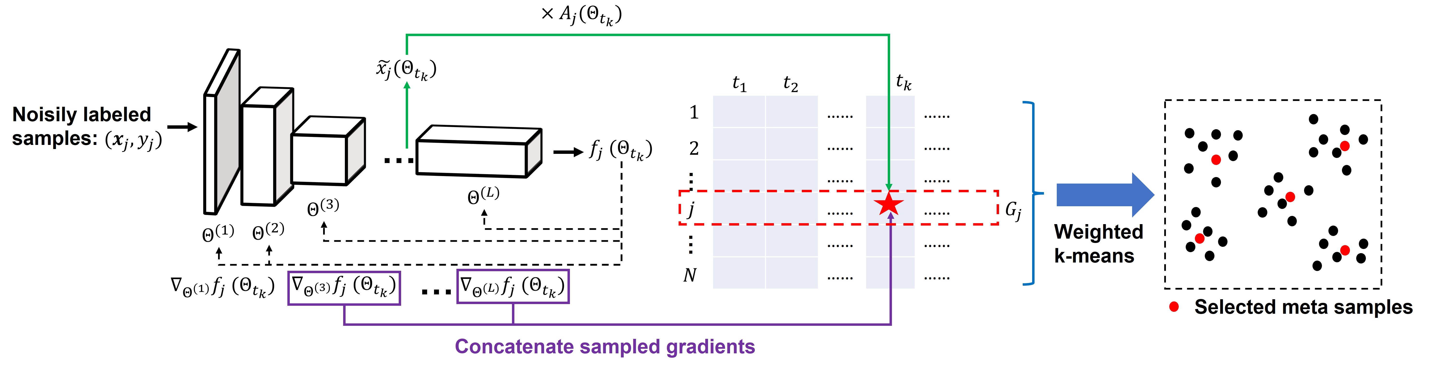
Figure 2: Overview of our methods, RBC and GBC. We use $\rightarrow$ (green colored arrow) and $\rightarrow$ (purple colored arrow) to denote the data flow of RBC and GBC respectively. Specifically, at each sampled time step $t_{k}$, for each input training sample $(\textbf{x}_{j},y_{j})$, RBC combines its feature vector from the input to the last layer of the model, $\tilde{\textbf{x}_{j}}$, and the coefficient, $\textbf{A}_{j}(\Theta_{t_{k}})$ (defined in Equation (12)) while GBC concatenate the gradients from the sampled layers in the model. We then concatenate the above calculated results from all the time steps $t_{1},t_{2},\dots$ to compose the input to weighted K-means clustering algorithm, $G_{j}$ (see the red dotted box), which is then used for determining the meta samples.

Solving MCO

MCO resembles the K-means clustering objective, so it is promising to solve it with the K-means clustering algorithm. As the first step toward this, MCO is transformed to the following form:

$$\begin{split}\text{MCO}&=\max_{\mathcal{C}}\sum_{j=1}^{N}\|G_{j}\|\sum_{i=1}^{M}\|C_{i}\|\cdot|\text{cosine}(G_{j},C_{i})|,\end{split}$$ (10)

which can be regarded as a weighted K-means clustering objective function. Specifically, the norm of each $C_{i}$ is used for re-weighting the cosine similarity between each training sample $j$ and each cluster centroid $i$, which is followed by re-weighting the overall similarity of each training sample $j$ to all cluster centroids with the norm of $G_{j}$. Further details on how to tailor the vanilla K-means clustering algorithm to solve MCO are presented in Appendix “Supplemental materials on the weighted K-means algorithm”. After $\mathcal{C}=\{C_{i}\}_{i=1}^{M}$ is identified by this weighted K-means algorithm, the samples closest to each cluster centroid are returned as the selected meta samples, $D_{\text{meta}}$.

Note that in Equation (9), collecting all $G_{j}$ is very expensive. This is because $j$ is over all training samples which can be very large, and $G_{j}$ depends on all $\Theta_{t}$, i.e., the model parameters at all iterations (see Equation (8)).

To address the above efficiency concerns, we firstly propose two methods, i.e., Representation-based clustering method (RBC) and Gradient-based clustering method (GBC) in Section “Representation-based clustering method (RBC)” and Section “Gradient-based clustering method (GBC)” respectively, for addressing the first concern. We further discuss how to sample from all $\Theta_{t}(t=1,2,\dots)$ in Section “Sampling model parameters from history” to handle the second concern.

Representation-based clustering method (RBC)

RBC is built upon the assumption that the gradient of the model parameters on the bottom layers (i.e. those layers closer to the input) is less significant than the ones in the last layer. Due to the vanishing gradient problem, this assumption usually holds in practice. As a consequence, we only consider the gradients from the last layer in Equation (9), leading to the following approximations on $G_{j}$:

$$\begin{split}G_{j}=\textbf{A}_{j}(\Theta_{t})\tilde{\textbf{x}_{j}}(\Theta_{t})^{\top},\end{split}$$ (11)

in which $\tilde{\textbf{x}_{j}}(\Theta_{t})$ represents the input to the last linear layer in the neural network model produced by the training sample $j$, while $\textbf{A}_{j}(\Theta_{t})$ is defined as follows:

$$\textbf{A}_{j}(\Theta_{t})=\text{softmax}(\Theta_{t}^{(-1)}\tilde{\textbf{x}_{j}}(\Theta_{t}))-\text{onehot}(y_{j})$$ (12)

in which $\Theta_{t}^{(-1)}$ represents the model parameters in the last layer. The detailed derivation of Equation (11) is included in Appendix “Derivation of Equation (11)”. Equation (11)-(12) shows that to obtain $G_{j}$, only forward passes on the models are needed, which makes this method very efficient.

Gradient-based clustering method (GBC)

Unlike RBC, GBC is applicable to general cases where the gradients generated by the bottom neural layers may be significant. To facilitate efficient evaluations of MCO, we importance sample the network layers from the model, such that we can obtain an unbiased estimation of Equation (9). Then $G_{j}$ is constructed by concatenating the gradients calculated in those sampled layers.

Specifically, first of all, the blue part of Equation (7) (which is the essential part of Equation (9)) can be rewritten in terms of a sum over the model parameters at each layer $l\in[1,2,\dots,L]$, i.e.:

$$\begin{split}&\langle\nabla_{\Theta}f_{\text{meta},i}(\Theta)|_{\Theta=\Theta_{t}},\nabla_{\Theta}f_{j}(\Theta)|_{\Theta=\Theta_{t}}\rangle\\ &=\left[\sum\nolimits_{l=1}^{L}\langle\nabla_{\Theta^{(l)}}f_{\text{meta},i}(\Theta)),\nabla_{\Theta^{(l)}}f_{j}(\Theta))\rangle\right]_{\Theta=\Theta_{t}},\end{split}$$ (13)

in which $\Theta^{(l)}$ represents the model parameters at the $l^{th}$ layer. Then the above formula could be rewritten as follows:

$$\begin{split}&\text{Equation }\eqref{eq: inner_prod_by_layer}\\ &=A\cdot\left[\sum_{l=1}^{L}\frac{A^{(l)}}{A}\langle\frac{\nabla_{\Theta^{(l)}}f_{\text{meta},i}(\Theta)}{\sqrt{A^{(l)}}},\frac{\nabla_{\Theta^{(l)}}f_{j}(\Theta)}{\sqrt{A^{(l)}}}\rangle\right]_{\Theta=\Theta_{t}},\end{split}$$ (14)

in which, $A^{(l)}=\|\frac{1}{N}\sum_{j=1}^{N}\nabla_{\Theta^{(l)}}f_{j}(\Theta)\|_{F}^{2}$ and $A=\sum_{l=1}^{L}A^{(l)}$

Then we can conduct importance sampling (with replacement) on the $L$ innermost sums in Equation (14) for several times (say 5 times), in which the probability of selecting the $l^{th}(l=1,2,\dots,L)$ term is $A^{(l)}/A$. This leads to an unbiased estimation of Equation (14) and significant speed-ups.

Sampling model parameters from history

It is worth noting that $\Theta_{t}$ is unknown before we obtain all meta samples (see Equation (2)-(4)), but it is essential for determining the meta samples (see Equation (7)). Therefore, we propose to cache the model parameter $\tilde{\Theta}_{t}(t=1,\dots,T)$ during the training process without any available meta samples, which is regarded as an approximation of $\Theta_{t}$.

In addition, as mentioned above, $G_{j}$ depends on the model parameters from all the time steps, which is thus very expensive to evaluate. We uniformly sample several time steps, instead of using all $\tilde{\Theta}_{t}$, to get an unbiased estimation of MCO.

In the end, we visually present both RBC and GBC equipped with this sampling technique in Figure 2 and include their pseudo-code in Algorithm 3 in Appendix “Details of the adapted K-means algorithm”.

Applications

We demonstrate the effectiveness of our methods for two applications, i.e., re-weighting a training set with noisy labels and re-weighting an imbalanced training set. In what follows, we discussed how to tailor RBC and GBC to these two applications.

Re-weighting a training set with noisy labels

To re-weight a noisily labeled training set, we can select a subset of meta samples from the training set and obtain their clean labels from human annotators. Note that for RBC and GBC, the evaluation of the gradients depend on the clean labels of the meta samples while these clean labels are obtained from human annotators after RBC or GBC is invoked. To address this chicken or the egg issue, we observe that if the loss function is the cross-entropy loss, then the sample-wise gradient, $\nabla_{\Theta}f_{j}(\Theta)$, can be broken into two parts, the label-free part and the label-dependent part. Due to the unavailability of the clean labels, we therefore only leverage the label-free part as the input to RBC and GBC.

Although we only use the label-free part, in Appendix “Analysis of the gradient with and without label-free part” (see Theorem 2), we theoretically analyze under what conditions the label-dependent part is insignificant to determining which cluster each training sample belongs to after the weighted k-means clustering algorithm is invoked. Those conditions are satisfied by a large portion of the training samples through our empirical studies (see Appendix “Supplemental experiments”), thus justifying the effectiveness of discarding the label-dependent part.

Re-weighting a training set with a class-imbalance

As indicated by (Shu et al. 2019), the meta re-weighting algorithm can also be leveraged for re-weighting class-imbalanced training sets. Unlike the case where the labels are noisy, we assume clean labels in the class-imbalanced training set. As a consequence, we evaluate the sample-wise gradient $\nabla_{\Theta}f_{j}(\Theta)$ as a whole rather than removing the label-dependent part from it.

Experiments

We demonstrate the effectiveness of our methods for training deep neural nets on image classification datasets, MNIST (Deng 2012), CIFAR-10 (Krizhevsky, Hinton et al. 2009) and CIFAR-100 (Krizhevsky, Hinton et al. 2009), and Imagenet-10 (Russakovsky et al. 2015). By following (Shu et al. 2019) and (Ren et al. 2018), we consider the occurrence of noisy labels and class imbalance respectively on the training set. All the code is publicly available.

Table 1: Test accuracy on MNIST, CIFAR-10 and CIFAR-100 dataset with noise rate 60%

Dataset	MNIST	CIFAR-10		CIFAR-100		Imagenet-10
Noise type	adversarial	uniform	adversarial	uniform	adversarial	uniform	adversarial
Base model	51.74$\pm$1.52	77.74$\pm$1.22	40.24$\pm$0.39	43.63$\pm$2.30	27.15$\pm$0.40	72.22	38.00
Random	85.67$\pm$0.90	73.56$\pm$0.40	76.02$\pm$2.01	42.30$\pm$4.68	45.33$\pm$1.70	93.33	59.77
Certain	81.84$\pm$0.89	74.76$\pm$1.07	70.78$\pm$5.00	45.95$\pm$4.20	47.06$\pm$2.10	91.20	58.22
Uncertain	76.38$\pm$0.54	73.83$\pm$0.24	74.45$\pm$6.10	36.67$\pm$0.20	44.65$\pm$0.65	85.22	51.00
Fine-tuning	53.39$\pm$1.22	78.46$\pm$2.10	23.07$\pm$7.58	25.28$\pm$1.13	24.88$\pm$1.10	70.44	35.67
TA-VAAL	79.31$\pm$0.23	72.89$\pm$0.82	61.46$\pm$4.65	31.07$\pm$2.56	38.79$\pm$0.86	86.34	43.26
craige	92.84$\pm$0.14	78.77$\pm$0.86	78.55$\pm$1.03	39.85$\pm$1.23	44.61$\pm$1.21	88.90	61.00
RBC-K	93.78$\pm$0.61	77.91$\pm$1.43	75.71$\pm$1.22	49.32$\pm$0.35	49.51$\pm$0.43	91.33	54.67
RBC	93.00$\pm$1.01	80.15$\pm$0.25	79.20$\pm$0.64	49.56$\pm$0.53	50.60$\pm$1.51	94.22	63.67
GBC	94.26$\pm$0.24	80.36$\pm$0.96	80.88$\pm$1.46	50.88$\pm$1.90	53.14$\pm$1.33	94.00	63.67

Experimental set-up

For the MNIST dataset, we train a LeNet model (LeCun et al. 1998) and for CIFAR-10, CIFAR-100 and Imagenet-10 dataset, we train a ResNet-34 model (He et al. 2016). All the hyper-paremters are reported in Appendix “Supplemental experiments”.

Dataset	CIFAR-10	CIFAR-100
BaseModel	61.45$\pm$0.60	28.14$\pm$0.57
Random	65.96$\pm$1.74	29.29$\pm$0.46
Uncertain	64.46$\pm$1.20	28.39$\pm$0.21
Certain	66.05$\pm$1.19	28.52$\pm$0.15
Fine-tuning	60.04$\pm$1.69	29.73$\pm$0.06
TA-VAAL	61.58$\pm$1.21	30.89$\pm$1.09
craige	66.60$\pm$0.89	29.56$\pm$1.46
RBC-K	65.96$\pm$1.02	30.77$\pm$1.23
RBC	68.18$\pm$1.58	31.78$\pm$1.10
GBC	67.37$\pm$1.51	33.87$\pm$0.66

Table 2: Test performance on imbalanced CIFAR-10 and CIFAR-100 dataset with imbalanced factor 200

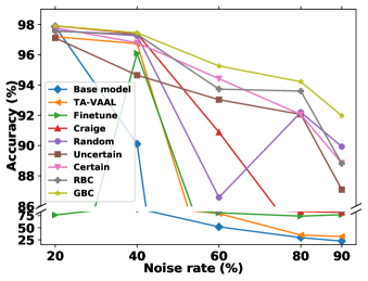
Figure 3: Test performance on MNIST dataset with varied noisy rate

Noisy label experiments

We first study how our methods perform in the presence of two types of label noise, i.e., uniform noise and adversarial noise:

• uniform noise: all labels can be uniformly flipped at random to any other label with probability $p/100$, in which $p$ is a percent specified by users. This has been explored in (Shu et al. 2019) and (Ren et al. 2018);

• adversarial noise: the labels for a subset of samples, chosen at random, are determinisitcally mapped to another label (e.g., selected samples with label 0 are all given label 1). This is meant to simulate an extreme case where the labels are adversarially flipped and has been explored in some prior works (e.g., (Li et al. 2022))

We present the results with one fixed noise rate, $p=60$, for both types of noise on MNIST, CIFAR and Imagenet-10 and the effect of varied $p$ is also explored on the MNIST dataset (see Figure 3). Surprisingly, we found that 60% uniform noise only reduces the model accuracy on MNIST by a few percent. We therefore only report the results on MNIST with adversarial noise. Throughout this experiment, we compare RBC and GBC against the following baseline methods:

• Random selection (Random): We uniformly at random select meta samples from the training set;

• Fine-tuning: We fine-tune the model using only the selected meta samples, selected by Random;

• Active learning: We select meta samples using 1) Uncertainty based selection (Uncertain) (Lewis and Gale 1994) by selecting the most uncertain training samples, 2) Certainty based selection (Certain) by selecting the most certain training samples and 3) two state-of-the-art active learning solutions, Task-Aware Variational Adversarial Active Learning (TA-VAAL) (Kim et al. 2021) and craige (craige) (Mirzasoleiman, Bilmes, and Leskovec 2020)

• RBC-k: We use the original K-means clustering algorithm rather than the weighted version proposed in Section “Solving MCO” to determine the meta samples in RBC.

Note that for both of our methods and the above baseline methods, the labels of the selected meta samples are cleaned by human annotators, which is simulated by replacing their noisy labels with ground-truth labels. This thus justifies the use of the perfectly labeled benchmark datasets (rather than real datasets with unreliable labels). As a result, for fair comparison, our methods and the above baseline methods share the same labeling budget, which is set as 20, 50, 200 and 50 for MNIST, CIFAR-10, CIFAR-100 and Imagenet-10 respectively (which includes the labeled samples in the pre-training phase). We pre-train the models by running the meta re-weighting algorithm with small amount of randomly selected meta samples (10 for MNIST, 10 for CIFAR-10, 50 for CIFAR-100 and 10 for Imagenet-10) since selecting those meta samples one time leads to sub-optimal performance, which is applied to all the baseline methods for fair comparison.

Table 3: The AUC score of the sample weights on MNIST with noise rate 80%

Method	All	Boundary
Random	0.922	0.589
RBC	0.958	0.775
GBC	0.949	0.854

Overall performance

We present the test accuracy in Table 1 after running the meta re-weighting algorithm with meta samples selected by different methods. As indicated by this table, the clustering-based methods, RBC-k, RBC and GBC can significantly outperform other methods in most cases and the performance gains are up to 6% (see the performance difference between GBC and Certain in column “adversarial” of CIFAR-100 dataset). Furthermore, RBC consistently outperforms RBC-K, which suggests the weighted K-means algorithm is capable of identifying a better set of meta samples than the original K-means algorithm.

Efficiency of RBC

We also observe a trade-off between performance and speed when comparing GBC and RBC. According to Table 1, GBC performs better than RBC in most cases while the former is slower than the latter (2.5 hours VS 3 mins) to construct $G_{j}$. Note that the running time of RBC is negligible in comparison to the running time of the meta re-weighting algorithm, which is around 4 mins per epoch and there are hundreds of epochs in total.

Robustness against varied noise rate

As indicated by Figure 3, both RBC and GBC outperform all the baseline methods across all the noise rates and the performance gains become even larger with more samples being noisily labeled (up to 2%). This indicates the robustness of our methods against a varied level of label noise.

Sample weight distributions

Recall that our methods depend on the assumption that larger updates to the sample weights will more effectively result in the weights of the noisy and clean samples approaching 0 and 1 respectively. We therefore empirically verify this assumption by inspecting the sample weights learned by Random, RBC and GBC. Specifically, we calculate the AUC between the learned sample weights and the cleanness of the sample labels (1 for clean while 0 for corrupt). We report this quantity for MNIST with 80% noisy labels in Table 3 for the entire training set and for the 1000 samples nearest to the decision boundary. As Table 3 shows, the AUC of RBC and GBC are significantly higher than that of Random, especially for those samples near the boundary, thus suggesting the capability for RBC and GBC to better distinguish between clean and noisy samples. This could thus explain why RBC and GBC achieve superior performance according to Table 3, thereby verifying our assumption.

Class imbalance experiments

For evaluating our method on class imbalanced data, we follow (Cui et al. 2019) to produce the long-tailed CIFAR dataset. Specifically, we down-sample some classes so that the ratio between the number of training samples in the largest class and that in the smallest one (which is denoted the imbalance factor) is large. In Table 2, we report the results with imbalance factor 200 on CIFAR-10 and CIFAR-100 dataset. As shown in Table 2, our method, RBC, outperforms all the baseline methods for CIFAR-10 and CIFAR-100  and the performance gain is up to 3.10%.

Other experimental results

Due to the space limit, all other experimental results are presented in Appendix: “Supplemental experiments”, including the experiments with real labeling noise on CIFAR dataset, the effect of the pre-training phase, the effect of varied number of meta samples, the effect of the number of sampled gradients in RBC and GBC (recall that both approximate Equation (10) through sampling according to Section: “Solving MCO”), and some qualitative studies.

Conclusion

In this work, we propose a clustering-based framework for selecting pivotal samples to improve performance of meta re-weighting in the presence of various defects on training data. Based on our theoretical analysis, we show that selecting pivotal samples can be reduced to a weighted K-means algorithm under reasonable assumptions. To efficiently evaluate this algorithm we propose two methods, RBC and GBC, which can balance the computational efficiency and prediction performance. Through empirical studies on noisily labeled and class-imbalanced image classification benchmark datasets, we can demonstrate that our technique could select a better set of pivotal samples for meta re-weighting algorithm than other sample selection techniques, thereby resulting in better model performance.

Appendix A Appendix: more related work

Extra related work on Shapley-value based data valuation

Due to the space limit of the main paper, we provide here a more extensive discussion on the existing data valuation literature, in particular, the works based on Data Shapley value ghorbani2019data. We notice that sim2022data summarized the recent progress in this area. However, as noted by sim2022data, these solutions are not scalable to large datasets due to the high computational overhead of data Shapley. It is worth noting that although these solutions, e.g., xu2021validation, sim2020collaborative, xu2021gradient, claim that they are applicable to realistic large datasets, they only study the data Shapley value of several “partitions” of the entire dataset and the number of partitions is typically smaller than 10. In contrast, to identify meta samples for the meta re-weighting algorithm, we need to compute the value of each individual training sample and thus the number of “partitions” is equivalent to the number of training samples, which is typically very large. This thus indicates that all the existing data Shapley dependent solutions are computationally intractable for our problem. Although there have been many recent attempts to approximately but efficiently compute data Shapley values, e.g., jia2019towards, yan2021if, jia12efficient, they are still far from being practical solutions since they either explicitly assume that the models have certain properties, which may not hold for general neural nets (e.g., jia2019towards, jia12efficient), or still require repetitive training (e.g., yan2021if). As a consequence, it is still an open challenge to efficiently compute data Shapley values for each sample in large datasets for general neural nets sim2022data.

In addition, note that xu2021validation proposes a data valuation metric without relying on the performance on the validation set, which, however, is built upon the data Shapley value, thus suffering from the efficiency issue as mentioned above.

Appendix B Appendix: Extra algorithmic details

Supplemental materials on the weighted K-means algorithm

In section “Solving MCO”, we discussed adapting the vanilla K-means clustering algorithm for solving MCO, which is presented in details in this section.

Input: A set of gradient vectors $\{G_{j}\}_{j=1}^{N}$
output: A set of cluster centroids $\{C_{i}\}_{i=1}^{M}$

1:  Randomly initialize $\{C_{i}\}_{i=1}^{M}$

2:  while not converged do

3:     Assignment step: Assign the sample $j$ to the cluster $\hat{i}$ such that $\hat{i}=\text{argmax}_{i}\{\|C_{i}\|\text{cosine}(G_{j},C_{i})\}_{i=1}^{M}$.

4:     Update step: Update the cluster centroid $j$ by Equation (S2).

5:  end while

Algorithm 1 A weighted K-means clustering algorithm for solving MCO

Input:A training set $D_{\text{train}}=\{(\textbf{x}_{i},y_{i})\}_{i=1}^{N}$, the total number of training iterations, $T$, the number of the randomly sampled meta samples in the warm-up phase, $M_{0}$, and a model with model parameter $\Theta$
Output:A set of meta samples $D_{\text{meta}}$

  Initialize $D_{\text{meta}}=\{\}$ /* Warm-up phase*/

  Randomly sample $M_{0}$ meta samples and add them into $D_{\text{meta}}$

  Run meta re-weighting algorithm with $D_{\text{meta}}$ as the meta sample set, resulting in a list of model parameters $\{\tilde{\Theta}_{t}\}_{t=1}^{T}$ at each iteration.

  while more validation samples are needed do

     Remove those training samples that are close to $D_{\text{meta}}$ (the similarity measure is the weighted cosine similarity defined in Equation (S1))

     Repetitively run Algorithm 1 until there is no empty clusters, in which $\{G_{j}\}_{j=1}^{N}$ is computed with RBC or GBC, and parameterized by $\{\tilde{\Theta}_{t}\}_{t=1}^{T}$. Suppose this results in cluster centroids $\{C_{i}\}_{i=1}^{M}$

     For each $C_{i}(i=1,2,\dots,M)$, add the closest training sample to this centroid into $D_{\text{meta}}$

     Run meta re-weighting algorithm with $D_{\text{meta}}$ as the meta sample set, resulting in a list of model parameters $\{\Theta_{t}\}_{t=1}^{T}$ at each iteration.

     $\{\tilde{\Theta}_{t}\}_{t=1}^{T}:=\{{\Theta}_{t}\}_{t=1}^{T}$

  end while

Algorithm 2 K-means clustering based meta sample selection

Input:A set of model parameters $\{\Theta_{t}\}_{t=1}^{T}$, the epoch $t^{*}$ with best validation performance
Output:$\{G_{j}\}_{j=1}^{N}$

  Uniformly sample $K$ models from $\{\Theta_{t}\}_{t=t^{*}+1}^{T}$, resulting in $\{\Theta_{t_{k}}\}_{k=1}^{K}$ where $t^{*}<t_{1}<t_{2}<\dots<t_{K}$

  Initialize $\{G_{j}\}_{j=1}^{N}$ so that $G_{j}=[]$ for all $j$.

  for $k=1$ to $K$ do

     if RBC then

        for $j=1$ to $N$ do

           Append $\textbf{A}_{j}(\Theta_{t_{k}})\tilde{\textbf{x}_{j}}(\Theta_{t_{k}})^{\top}$ to $G_{j}$ according to Equation (11)

        end for

     else if GBC then

        Compute $A^{(l)}(\Theta_{t_{k}})$ and $A(\Theta_{t_{k}})$ for all $l(l=1,2,\dots,L)$ as described in Section “Gradient-based clustering method (GBC)”

        for $j=1$ to $N$ do

           Conduct importance sampling from $[\nabla_{\Theta^{(1)}}f_{j}(\Theta_{t_{k}})\dots\nabla_{\Theta^{(L)}}f_{j}(\Theta_{t_{k}})]$ with sampling probability $[\frac{A^{(1)}(\Theta_{t_{k}})}{A(\Theta_{t_{k}})},\frac{A^{(2)}(\Theta_{t_{k}})}{A(\Theta_{t_{k}})},\dots,\frac{A^{(L)}(\Theta_{t_{k}})}{A(\Theta_{t_{k}})}]$, resulting in a list of gradients from $R$ layers: $\text{Grad}_{j}=[\nabla_{\Theta^{(l_{1})}}f_{j}(\Theta_{t_{k}}),\nabla_{\Theta^{(l_{2})}}f_{j}(\Theta_{t_{k}}),\dots,\nabla_{\Theta^{(l_{R})}}f_{j}(\Theta_{t_{k}})]$

           Append $\text{Grad}_{j}$ to $G_{j}$

        end for

     end if

  end for

  for $j=1$ to $N$ do

     Organize $G_{j}$ as a block matrix

  end for

Algorithm 3 RBC and GBC

Details of the adapted K-means algorithm

We tailor the vanilla K-means clustering algorithm to efficiently solve Equation (10). Note that the K-means clustering algorithm is composed of two steps, i.e., the assignment step and the update step, which are conducted alternatively until convergence. In the assignment step of the modified K-means clustering algorithm, we follow the same principle of the vanilla K-means clustering algorithm. Specifically, we assign each training sample to its nearest cluster centroid, where the similarity between each training sample $j$ and each cluster centroid $i$ is the cosine similarity weighted by the norm of the centroid $C_{i}$:

$$\begin{split}\|C_{i}\|\cdot|\text{cosine}(G_{j},C_{i})|\end{split}$$ (S1)

After each training sample $j$ is assigned to a certain cluster centroid $C_{i}$, we proceed to update the cluster centroids in the update step given their assigned training samples. Indeed, according to Equation (10), we conduct clustering on the normalized gradients, $\frac{G_{j}}{\|G_{j}\|}$, rather than $G_{j}$ itself. Plus, since the overall similarity between each training sample $j$ and all clustering centroids is weighted by the norm of $G_{j}$, we therefore update the cluster centroids by leveraging the following formula:

$$\begin{split}C_{i}\leftarrow\sum\nolimits_{j\in\text{cluster }i}\frac{\|G_{j}\|\cdot\frac{G_{j}}{\|G_{j}\|}}{\sum\nolimits_{j\in\text{cluster }i}\|G_{j}\|}=\sum\nolimits_{j\in\text{cluster }i}\frac{G_{j}}{\sum\nolimits_{j\in\text{cluster }i}\|G_{j}\|},\end{split}$$ (S2)

in which, the cluster centroid $C_{i}$ is updated as the weighted mean of all the normalized samples that are assigned to this cluster.

The value of each $G_{j}$ is computed based on if RBC or GBC is used. The details are summarized in Algorithm 3.

In the end, we summarize this adapted K-means clustering algorithm in Algorithm 1.

Determining number of clusters and continuously adding meta samples

In this section, we further discuss how to determine the number of clusters and how to continuously add meta samples while the meta re-weighting algorithm is repetitively invoked.

First of all, we assume that the number of clusters, $M$, could be provided by the users. However, we observe that given an inappropriately large $M$, empty clusters are often generated, meaning that no samples are assigned to these clusters. Suppose that there are $M_{\text{empty}}$ empty clusters in total, we therefore restart the K-means clustering algorithm with the number of clusters as $M-M_{\text{cluster}}$. This process is repeated until there are no empty clusters. We then identify meta samples with the resulting clusters, which are used in the meta re-weighting algorithm. Suppose we get model parameters ${\Theta}_{t}(t=1,2,\dots,T)$ from the meta re-weighting algorithm, we can also optionally run RBC or GBC again by leveraging ${\Theta}_{t}$ so that we can add more meta samples. This process is summarized in Algorithm 2. Note that in the subsequent invocation of RBC or GBC, we remove a certain portion of training samples (e.g., half of them) that are closest to the existing meta samples and only cluster the remaining training samples to discover new meta samples.

Appendix C Appendix: Mathematical details

Derivation of Equation (6)

First of all, we compute the partial gradient of Equation (2) with respect to $w_{j}$, i.e.:

$$\begin{split}\frac{\partial\hat{\Theta}(\textbf{W}_{t})}{\partial w_{j}}&=\frac{\partial}{\partial w_{j}}[\Theta_{t}-\alpha_{t}\cdot\frac{1}{N}\sum\nolimits_{r=1}^{N}w_{r,t}\nabla_{\Theta}f_{r}(\Theta)|_{\Theta=\Theta_{t}}]\\ &=-\frac{\alpha_{t}}{N}\nabla_{\Theta}f_{j}(\Theta)|_{\Theta=\Theta_{t}},\end{split}$$ (S3)

which utilizes the fact that except for $w_{j,t}\nabla_{\theta}f_{j}(\Theta)$, all the other terms in Equation (2) do not depend on the weight $w_{j,t}$.

In addition, we utilize chain rule on the gradient of Equation (3), leading to:

$$\begin{split}&\nabla_{w_{j}}f_{\text{meta},i}(\hat{\Theta}(\textbf{W}_{t}))=\langle\nabla_{\Theta}f_{\text{meta},i}(\Theta)|_{\Theta=\hat{\Theta}(\textbf{W}_{t})},\frac{\partial\hat{\Theta}(\textbf{W}_{t})}{w_{j}}\rangle\\ &=-\frac{\alpha_{t}}{N}\langle\nabla_{\Theta}f_{\text{meta},i}(\Theta)|_{\Theta=\hat{\Theta}(\textbf{W}_{t})},\nabla_{\Theta}f_{j}(\Theta)|_{\Theta=\Theta_{t}}\rangle\end{split}$$ (S4)

Derivation of Equation (11)

In the main paper, we have used $\langle,\rangle$ to denote the Frobenius inner product between matrices. But in the following analysis, the inner products between vectors will also appear, which are also conventionally denoted as $\langle,\rangle$. Therefore, to distinguish between these two types of inner products in what follows, we use $\langle,\rangle_{F}$ rather than $\langle,\rangle$ to represent the Frobenius inner product between matrices while $\langle,\rangle$ is used for representing the inner product between vectors.

First of all, suppose the loss function is cross-entropy loss, then we could have the following lemma for this loss:

Lemma 1.

For cross-entropy loss, we can write it as the following form:

$$L(\textbf{x},y)=\log(\frac{\exp^{-x_{j}}}{\sum_{k=1}^{m}\exp^{-x_{k}}}),$$ (S5)

in which we assume that $y=j\ (j\in\{1,2,\dots,m\})$ and $\textbf{x}=[x_{1},x_{2},\dots,x_{m}]$ is a vector of length $m$. Then the gradient of $L(\textbf{x},y)$ with respect to the input x could be split into two parts, i.e. the label-dependent part and the label-free part.

Proof.

The gradient of $L(\textbf{x},y)$ with respect to x could be derived as follows:

$$\frac{\partial L(\textbf{x},y)}{\partial\textbf{x}}=[\frac{\partial L(\textbf{x},y)}{\partial x_{1}},\frac{\partial L(\textbf{x},y)}{\partial x_{2}},\dots,\frac{\partial L(\textbf{x},y)}{\partial x_{r}},\dots,\frac{\partial L(\textbf{x},y)}{\partial x_{m}}]^{\top},$$

in which,

$$\frac{\partial L(\textbf{x},y)}{\partial x_{r}}=\begin{cases}\frac{\exp^{-x_{r}}}{\sum_{k=1}^{m}\exp^{-x_{k}}},r\neq y\\ \frac{\exp^{-x_{r}}}{\sum_{k=1}^{m}\exp^{-x_{k}}}-1,r=y\end{cases}$$

As a consequence, $\frac{\partial L(\textbf{x},y)}{\partial\textbf{x}}$ could be written as:

$$\begin{split}\frac{\partial L(\textbf{x},y)}{\partial\textbf{x}}&=[\frac{\partial L(\textbf{x},y)}{\partial x_{1}},\frac{\partial L(\textbf{x},y)}{\partial x_{2}},\dots,\frac{\partial L(\textbf{x},y)}{\partial x_{r}},\dots,\frac{\partial L(\textbf{x},y)}{\partial x_{m}}]^{\top}\\ &=[\frac{\exp^{-x_{1}}}{\sum_{k=1}^{m}\exp^{-x_{k}}},\frac{\exp^{-x_{2}}}{\sum_{k=1}^{m}\exp^{-x_{k}}},\dots,\frac{\exp^{-x_{r}}}{\sum_{k=1}^{m}\exp^{-x_{k}}},\dots,\frac{\exp^{-x_{m}}}{\sum_{k=1}^{m}\exp^{-x_{k}}}]^{\top}-\text{onehot}(j)\\ &=\underbrace{\text{softmax}(\textbf{x})}_{\textit{label free part}}-\underbrace{\text{onehot}(y)}_{\textit{label dependent part}}\end{split}$$ (S6)

∎

Note that when we only consider the gradient of the last layer, whose parameters are denoted as $\Theta^{(-1)}$, $f_{j}(\Theta)$ and $f_{\text{meta},i}(\Theta)$ could be represented as:

$$f_{j}(\Theta)=L(\textbf{x}^{\text{last out}}_{j}(\Theta),y_{j})=L(\Theta^{(-1)}\tilde{\textbf{x}_{j}}(\Theta),y_{j}),f_{\text{meta},i}(\Theta)=L(\textbf{x}^{\text{last out}}_{\text{meta},i}(\Theta),y_{\text{meta},i})=L(\Theta^{(-1)}\tilde{\textbf{x}_{\text{meta},i}}(\Theta),y_{\text{meta},i}).$$

Recall that in Section “Representation-based clustering method (RBC)” and Section “Re-weighting a training set with noisy labels”, we use $\textbf{x}^{\text{last out}}_{j}(\Theta)$ and $\tilde{\textbf{x}_{j}}(\Theta)$ to denote the input of the last linear layer and the input of the softmax layer (i.e. the output of the last linear layer) given the training sample $j$. Similarly, $\textbf{x}^{\text{last out}}_{\text{meta},i}(\Theta)$ and $\tilde{\textbf{x}_{\text{meta},i}}(\Theta)$ represent the input and the output of the last linear layer given the meta sample $i$.

Then we could derive the gradient of $f_{j}(\Theta)$ (same for $f_{\text{meta},i}(\Theta)$) with respect to the vectorized $\Theta^{(-1)}$ by leveraging the chain rule, leading to:

$$\nabla_{\text{vec}(\Theta^{(-1)})}f_{j}(\Theta)=\frac{\partial\textbf{x}^{\text{last out}}_{j}(\Theta)}{\partial\text{vec}(\Theta^{(-1)})}\cdot\frac{\partial L(\textbf{x}^{\text{last out}}_{j}(\Theta),\tilde{y_{j}})}{\partial\textbf{x}^{\text{last out}}_{j}(\Theta)}.$$ (S7)

By leveraging Lemma 1, the above formula could be rewritten as:

$$\nabla_{\text{vec}(\Theta^{(-1)})}f_{j}(\Theta)=\frac{\partial\textbf{x}^{\text{last out}}_{j}(\Theta)}{\partial\text{vec}(\Theta^{(-1)})}\cdot[\text{softmax}(\Theta^{(-1)}\tilde{\textbf{x}_{j}}(\Theta))-\text{onehot}(y_{j})]$$

and for $\frac{\partial\textbf{x}^{\text{last out}}_{j}(\Theta)}{\partial\text{vec}(\Theta^{(-1)})}$, it could be further derived as follows by utilizing the calculus on block matrix:

$$\frac{\partial\textbf{x}^{\text{last out}}_{j}(\Theta)}{\partial\text{vec}(\Theta^{(-1)})}=\frac{\partial\Theta^{(-1)}\tilde{\textbf{x}_{j}}(\Theta)}{\partial\text{vec}(\Theta^{(-1)})}=[\tilde{\textbf{x}_{j}}(\Theta)\otimes\textbf{I}]^{\top}=[\tilde{\textbf{x}_{j,1}}(\Theta)\textbf{I},\tilde{\textbf{x}_{j,2}}(\Theta)\textbf{I},\dots\tilde{\textbf{x}_{j,m}}(\Theta)\textbf{I}]^{\top}$$

in which $\textbf{x}_{j,r}(\Theta)$ denotes the $r_{th}$ entry of the vector $\textbf{x}_{j}(\Theta)$ and $\otimes$ denotes the Kronecker product henderson1983history on two matrices.

We then plug the above formula into Equation (S7), resulting in:

$$\nabla_{\text{vec}(\Theta^{(-1)})}f_{j}(\Theta) =[\tilde{\textbf{x}_{j,1}}(\Theta)\textbf{I},\tilde{\textbf{x}_{j,2}}(\Theta)\textbf{I},\dots\tilde{\textbf{x}_{j,m}}(\Theta)\textbf{I}]^{\top}\cdot[\text{softmax}(\Theta^{(-1)}\tilde{\textbf{x}_{j}}(\Theta))-\text{onehot}(y_{j})]$$

$$=\text{vec}(\left[\text{softmax}(\Theta^{(-1)}\tilde{\textbf{x}_{j}}(\Theta))-\text{onehot}(y_{j})\right]\tilde{\textbf{x}_{j}}(\Theta)^{\top}),$$

Recall that in Section “Representation-based clustering method (RBC)”, we use $\textbf{A}_{j}(\Theta)$ to denote $\text{softmax}(\Theta^{(-1)}\tilde{\textbf{x}_{j}}(\Theta))-\text{onehot}(y_{j})$. Therefore, the above formula could be rewritten as:

$$\begin{split}\nabla_{\text{vec}(\Theta^{(-1)})}f_{j}(\Theta)=\text{vec}(\textbf{A}_{j}(\Theta)\tilde{\textbf{x}_{j}}(\Theta)^{\top})\end{split}$$

Similarly, the following equation holds for the meta sample $i$:

$$\begin{split}\nabla_{\text{vec}(\Theta^{(-1)})}f_{\text{meta},i}(\Theta)=\text{vec}(\textbf{A}_{\text{meta},i}(\Theta)\tilde{\textbf{x}_{\text{meta},i}}(\Theta)^{\top})\end{split}$$

As a result, we can compute the inner product between $\nabla_{\text{vec}(\Theta^{(-1)})}f_{\text{meta},i}(\Theta)$ and $\nabla_{\text{vec}(\Theta^{(-1)})}f_{j}(\Theta)$ by leveraging the above two formulas, leading to:

$$\begin{split}\langle\nabla_{\text{vec}(\Theta^{(-1)})}f_{\text{meta},i}(\Theta),\nabla_{\text{vec}(\Theta^{(-1)})}f_{j}(\Theta)\rangle&=\langle\text{vec}(\textbf{A}_{j}(\Theta)\tilde{\textbf{x}_{j}}(\Theta)^{\top}),\text{vec}(\textbf{A}_{\text{meta},i}(\Theta)\tilde{\textbf{x}_{\text{meta},i}}(\Theta)^{\top})\rangle\\ &=\langle\textbf{A}_{j}(\Theta)\tilde{\textbf{x}_{j}}(\Theta)^{\top},\textbf{A}_{\text{meta},i}(\Theta)\tilde{\textbf{x}_{\text{meta},i}}(\Theta)^{\top}\rangle_{F}\end{split}$$

We can then plug the above formula into Equation (8), i.e. MSSO, leading to:

MSSO $$=\max_{D_{\text{meta}}}\sum\nolimits_{j=1}^{N}\left|\sum\nolimits_{i=1}^{M}\langle G_{j},G_{\text{meta},i}\rangle\right|$$

$$=\max_{D_{\text{meta}}}\sum\nolimits_{j=1}^{N}\left|\sum\nolimits_{i=1}^{M}\sum\nolimits_{\Theta_{t}}\langle\nabla_{\Theta}f_{j}(\Theta)|_{\Theta=\Theta_{t}},\nabla_{\Theta}f_{\text{meta},i}(\Theta)|_{\Theta=\Theta_{t}}\rangle\right|$$

$$=\max_{D_{\text{meta}}}\sum\nolimits_{j=1}^{N}\left|\sum\nolimits_{i=1}^{M}\sum\nolimits_{\Theta_{t}}\langle\nabla_{\text{vec}(\Theta)}f_{j}(\Theta)|_{\Theta=\Theta_{t}},\nabla_{\text{vec}(\Theta)}f_{\text{meta},i}(\Theta)|_{\Theta=\Theta_{t}}\rangle\right|$$

$$\approx\max_{D_{\text{meta}}}\sum\nolimits_{j=1}^{N}\left|\sum\nolimits_{i=1}^{M}\sum\nolimits_{\Theta_{t}}\langle\nabla_{\text{vec}(\Theta^{(-1)})}f_{j}(\Theta)|_{\Theta=\Theta_{t}},\nabla_{\text{vec}(\Theta^{(-1)})}f_{\text{meta},i}(\Theta)|_{\Theta=\Theta_{t}}\rangle\right|$$

$$=\max_{D_{\text{meta}}}\sum\nolimits_{j=1}^{N}\left|\sum\nolimits_{i=1}^{M}\sum\nolimits_{\Theta_{t}}\langle\textbf{A}_{j}(\Theta_{t})\tilde{\textbf{x}_{j}}(\Theta_{t})^{\top},\textbf{A}_{\text{meta},i}(\Theta_{t})\tilde{\textbf{x}_{\text{meta},i}}(\Theta_{t})^{\top}\rangle_{F}\right|$$

This thus concludes the derivation of Equation (11).

Proof of Theorem 1

Proof.

By utilizing the following property concerning the absolute values of the sum of two numbers stewart2011calculus:

$$|a+b|=||a|-|b||,\text{if }a\cdot b\leq 0,$$

the inner most sum in Equation (8) could be rewritten as follows:

$$|\sum\nolimits_{i=1}^{M}\langle G_{j},C_{i}\rangle|$$

$$=|\sum\nolimits_{\langle G_{j},C_{i}\rangle>0}\langle G_{j},C_{i}\rangle+\sum\nolimits_{\langle G_{j},C_{i}\rangle<0}\langle G_{j},C_{i}\rangle|$$

$$=||\sum\nolimits_{\langle G_{j},C_{i}\rangle>0}\langle G_{j},C_{i}\rangle|-|\sum\nolimits_{\langle G_{j},C_{i}\rangle<0}\langle G_{j},C_{i}\rangle||$$

Also, by utilizing the following property concerning the sum of the absolute value of two numbers stewart2011calculus:

$$|a|+|b|=|a+b|,\text{if }a\cdot b\geq 0$$

for the innermost sum in Equation (9) could be rewritten as follows:

$$\sum\nolimits_{i=1}^{M}|\langle G_{j},C_{i}\rangle|$$

$$=\sum\nolimits_{\langle G_{j},C_{i}\rangle>0}|\langle G_{j},C_{i}\rangle|+\sum_{\langle G_{j},C_{i}\rangle<0}|\langle G_{j},C_{i}\rangle|$$

$$=|\sum\nolimits_{\langle G_{j},C_{i}\rangle>0}\langle G_{j},C_{i}\rangle|+|\sum\nolimits_{\langle G_{j},C_{i}\rangle<0}\langle G_{j},C_{i}\rangle|$$

Then we compute the ratio between the above two formulas, leading to:

$$\begin{split}&\frac{|\sum\nolimits_{i=1}^{M}\langle G_{j},C_{i}\rangle|}{\sum\nolimits_{i=1}^{M}|\langle G_{j},C_{i}\rangle|}=\frac{||\sum\nolimits_{\langle G_{j},C_{i}\rangle>0}\langle G_{j},C_{i}\rangle|-|\sum\nolimits_{\langle G_{j},C_{i}\rangle<0}\langle G_{j},C_{i}\rangle||}{|\sum\nolimits_{\langle G_{j},C_{i}\rangle>0}\langle G_{j},C_{i}\rangle|+|\sum\nolimits_{\langle G_{j},C_{i}\rangle<0}\langle G_{j},C_{i}\rangle|}\\ &=\begin{cases}\frac{\frac{|\sum\nolimits_{\langle G_{j},C_{i}\rangle<0}\langle G_{j},C_{i}\rangle|}{|\sum\nolimits_{\langle G_{j},C_{i}\rangle>0}\langle G_{j},C_{i}\rangle|}-1}{\frac{|\sum\nolimits_{\langle G_{j},C_{i}\rangle<0}\langle G_{j},C_{i}\rangle|}{|\sum\nolimits_{\langle G_{j},C_{i}\rangle>0}\langle G_{j},C_{i}\rangle|}+1}=1-\frac{2}{\frac{|\sum\nolimits_{\langle G_{j},C_{i}\rangle<0}\langle G_{j},C_{i}\rangle|}{|\sum\nolimits_{\langle G_{j},C_{i}\rangle>0}\langle G_{j},C_{i}\rangle|}+1}&\text{if }|\sum\nolimits_{\langle G_{j},C_{i}\rangle<0}\langle G_{j},C_{i}\rangle|>|\sum\nolimits_{\langle G_{j},C_{i}\rangle>0}\langle G_{j},C_{i}\rangle|\\ \frac{\frac{|\sum\nolimits_{\langle G_{j},C_{i}\rangle>0}\langle G_{j},C_{i}\rangle|}{|\sum\nolimits_{\langle G_{j},C_{i}\rangle<0}\langle G_{j},C_{i}\rangle|}-1}{\frac{|\sum\nolimits_{\langle G_{j},C_{i}\rangle>0}\langle G_{j},C_{i}\rangle|}{|\sum\nolimits_{\langle G_{j},C_{i}\rangle<0}\langle G_{j},C_{i}\rangle|}+1}=1-\frac{2}{\frac{|\sum\nolimits_{\langle G_{j},C_{i}\rangle>0}\langle G_{j},C_{i}\rangle|}{|\sum\nolimits_{\langle G_{j},C_{i}\rangle<0}\langle G_{j},C_{i}\rangle|}+1}&\text{if }|\sum\nolimits_{\langle G_{j},C_{i}\rangle>0}\langle G_{j},C_{i}\rangle|>|\sum\nolimits_{\langle G_{j},C_{i}\rangle<0}\langle G_{j},C_{i}\rangle|\end{cases}\end{split}$$ (S8)

Then by leveraging the assumption of this Theorem, we know that:

$$\begin{cases}\frac{|\sum\nolimits_{\langle G_{j},C_{i}\rangle>0}\langle G_{j},C_{i}\rangle|}{|\sum\nolimits_{\langle G_{j},C_{i}\rangle<0}\langle G_{j},C_{i}\rangle|}>D&\text{ if }|\sum\nolimits_{\langle G_{j},C_{i}\rangle<0}\langle G_{j},C_{i}\rangle|>|\sum\nolimits_{\langle G_{j},C_{i}\rangle>0}\langle G_{j},C_{i}\rangle|\\ \frac{|\sum\nolimits_{\langle G_{j},C_{i}\rangle<0}\langle G_{j},C_{i}\rangle|}{|\sum\nolimits_{\langle G_{j},C_{i}\rangle>0}\langle G_{j},C_{i}\rangle|}>D&\text{ if }|\sum\nolimits_{\langle G_{j},C_{i}\rangle>0}\langle G_{j},C_{i}\rangle|>|\sum\nolimits_{\langle G_{j},C_{i}\rangle<0}\langle G_{j},C_{i}\rangle|\end{cases}$$

Therefore, Equation (S8) could be bounded as follows:

$$\text{Equation }\eqref{eq: theorem_bound_derivation_1} =\begin{cases}1-\frac{2}{\frac{|\sum\nolimits_{\langle G_{j},C_{i}\rangle<0}\langle G_{j},C_{i}\rangle|}{|\sum\nolimits_{\langle G_{j},C_{i}\rangle>0}\langle G_{j},C_{i}\rangle|}+1}&\text{if }|\sum\nolimits_{\langle G_{j},C_{i}\rangle<0}\langle G_{j},C_{i}\rangle|>|\sum\nolimits_{\langle G_{j},C_{i}\rangle>0}\langle G_{j},C_{i}\rangle|\\ 1-\frac{2}{\frac{|\sum\nolimits_{\langle G_{j},C_{i}\rangle>0}\langle G_{j},C_{i}\rangle|}{|\sum\nolimits_{\langle G_{j},C_{i}\rangle<0}\langle G_{j},C_{i}\rangle|}+1}&\text{if }|\sum\nolimits_{\langle G_{j},C_{i}\rangle>0}\langle G_{j},C_{i}\rangle|>|\sum\nolimits_{\langle G_{j},C_{i}\rangle<0}\langle G_{j},C_{i}\rangle|\end{cases}$$

$$>\begin{cases}1-\frac{2}{D+1}&\text{if }|\sum\nolimits_{\langle G_{j},C_{i}\rangle<0}\langle G_{j},C_{i}\rangle|>|\sum\nolimits_{\langle G_{j},C_{i}\rangle>0}\langle G_{j},C_{i}\rangle|\\ 1-\frac{2}{D+1}&\text{if }|\sum\nolimits_{\langle G_{j},C_{i}\rangle>0}\langle G_{j},C_{i}\rangle|>|\sum\nolimits_{\langle G_{j},C_{i}\rangle<0}\langle G_{j},C_{i}\rangle|\end{cases}$$

$$=\frac{D-1}{D+1}$$

In Section “Supplemental experiments”, we will calculate the value of $D$ empirically. Recall that the value of $D$ needs to be significantly larger than 1 so that solving MCO (i.e. Equation (9)) could end up with a reasonable approximation to the solution of MSSO (i.e. Equation (8)), which could be empirically justified on MNIST and CIFAR dataset.

∎

Generalization of our methods for ren2018learning

As discussed in Section “Background: the meta re-weighting algorithm”, our methods mainly utilize the meta-reweighting algorithm proposed in shu2019meta. However, we can show that our methods can also support other meta-reweighting algorithms, such as ren2018learning, which we illustrate in this section.

First of all, we notice that ren2018learning and shu2019meta mainly differ in how to update the sample weights at each time step. Specifically, we reformulate Equation (2)-Equation (4) according to ren2018learning as follows:

Meta re-weighting ren2018learning:

$$\hat{\Theta}(\textbf{W}_{t})=\Theta_{t}-\alpha_{t}\cdot\frac{1}{N}\sum\nolimits_{j=1}^{N}w_{j,t}\nabla_{\Theta}f_{j}(\Theta)|_{\Theta=\Theta_{t},w_{j,t}=0}$$ (S9)

$$\hat{w}_{j,t+1}=-\eta_{t}\cdot\frac{1}{M}\sum\nolimits_{i=1}^{M}\nabla_{w_{j,t}}f_{\text{meta},i}(\hat{\Theta}(\textbf{W}_{t}))|_{w_{j,t}=0}$$ (S10)

$$\hat{w}_{j,t+1}=\max\{\hat{w}_{j,t+1},0\},w_{j,t+1}=\text{normalize}([\hat{w}_{1,t+1},\hat{w}_{2,t+1},\dots,\hat{w}_{N,t+1}])$$ (S11)

$$\Theta_{t+1}=\Theta_{t}-\alpha_{t}\cdot\frac{1}{N}\sum\nolimits_{j=1}^{N}w_{j,t+1}\nabla_{\Theta}f_{j}(\Theta)|_{\Theta=\Theta_{t}},$$ (S12)

Recall that the intuition of our methods is to find meta samples so that each sample weight $w_{j}$ is effectively updated during the training process instead of staying close to its random initialization. Therefore, we hope to maximize the following cumulative gradients across all the samples during the entire training process, i.e.:

$$\max_{D_{\text{meta}}}\sum\nolimits_{\hat{\Theta}(\textbf{W}_{t})}\frac{1}{M}\sum\nolimits_{i=1}^{M}\nabla_{w_{j}}f_{\text{meta},i}(\hat{\Theta}(\textbf{W}_{t})),\text{for all $j=(1,2,\dots,N)$},$$ (S13)

Note that different from Equation (5), no absolute value is calculated in Equation (S13). Then by following the same derivation as Equation (6), we can get the following formula which is similar to Equation (7):

$$\begin{split}&\max_{D_{\text{meta}}}\sum\nolimits_{j=1}^{N}{\sum\nolimits_{\hat{\Theta}(\textbf{W}_{t}),\Theta_{t}}\sum\nolimits_{i=1}^{M}\langle\nabla_{\Theta}f_{\text{meta},i}(\Theta)|_{\Theta=\hat{\Theta}(\textbf{W}_{t})},\nabla_{\Theta}f_{j}(\Theta)|_{\Theta=\Theta_{t}}\rangle}\\ &\approx\max_{D_{\text{meta}}}\sum\nolimits_{j=1}^{N}{\sum\nolimits_{i=1}^{M}\sum\nolimits_{\Theta_{t}}\langle\nabla_{\Theta}f_{\text{meta},i}(\Theta)|_{\Theta=\Theta_{t}},\nabla_{\Theta}f_{j}(\Theta)|_{\Theta=\Theta_{t}}\rangle}.\\ \end{split}$$ (S14)

Again, the only difference between Equation (7) and Equation (S14) is the existence of the absolute value computation. As a result, when the meta-reweighting algorithm from ren2018learning is used, our methods, including both RBC and GBC, can be employed for selecting meta samples, except that the absolute value is not evaluated.

Analysis of the gradient with and without label-free part

According to Section “Re-weighting a training set with noisy labels”, in the presence of label noises, the sample-wise gradient $\nabla_{\Theta}f_{j}(\Theta)$ could be split into label-free part and the label-dependent part, which are represented as follows:

$$\begin{split}&\nabla_{\Theta}f_{j}(\Theta)=[\underbrace{\frac{\partial\textbf{x}^{\text{last out}}_{j}(\Theta)}{\partial\Theta}\cdot\text{softmax}(\textbf{x}^{\text{last out}}_{j}(\Theta))}_{\textit{label-free gradient}}-\underbrace{\frac{\partial\textbf{x}^{\text{last out}}_{j}(\Theta)}{\partial\Theta}\cdot\text{onehot}(y)}_{\textit{label-dependent gradient}}],\end{split}$$ (S15)

in which $\textbf{x}^{\text{last out}}_{j}(\Theta)$ represents the input of the softmax layer of the neural model. The derivation of Equation (S15) is discussed in Lemma 1 in Appendix “Derivation of Equation (11)”.

Recall that in Section “Re-weighting a training set with noisy labels”, we only focus on the label-free part in the sample-wise gradient, i.e., $\nabla_{\Theta}\widetilde{f_{j}(\Theta)}$. Therefore, by replacing $\nabla_{\Theta}f_{j}(\Theta)$ with $\nabla_{\Theta}\widetilde{f_{j}(\Theta)}$ and $\nabla_{\Theta}f_{\text{meta},i}(\Theta)$ with $\nabla_{\Theta}\widetilde{f_{\text{meta},i}(\Theta)}$ in Equation (9), the objective function becomes:

$$\max_{D_{\text{meta}}}(\sum_{j=1}^{N}\sum_{i=1}^{M}|\langle\widetilde{G_{j}},\widetilde{G_{\text{meta},i}}\rangle|),$$ (S16)

in which,

$$\widetilde{G_{j}}=\left[\nabla_{\Theta}\widetilde{f_{j}(\Theta)}|_{\Theta=\Theta_{1}}\cdots\nabla_{\Theta}\widetilde{f_{j}(\Theta)}|_{\Theta=\Theta_{t}}\cdots\right],\widetilde{G_{\text{meta},i}}=\left[\nabla_{\Theta}\widetilde{f_{\text{meta},i}(\Theta)}|_{\Theta=\Theta_{1}}\cdots\nabla_{\Theta}\widetilde{f_{\text{meta},i}(\Theta)}|_{\Theta=\Theta_{t}}\cdots\right]$$

In what follows, i.e., Theorem 2, we are going to show that with some assumptions, solving Equation (S16) can produce approximately the same clusters as the ones produced by solving Equation (9) where the sample labels are involved.

Theorem 2.

Suppose solving Equation (11) with the weighted K-means algorithm, i.e., Algorithm 1, assigns the training sample $j$ to the cluster centroid $c^{(j)}$. Then if the following assumptions hold for the training sample $i$:

1. The similarity between the training sample $j$ and the assigned centroid $c^{(j)}$, is greater than $\alpha_{j}$ and the similarity between each training sample $j$ and any other cluster centroid $i$ is smaller than $\beta_{j}$ ($\alpha_{j}>\beta_{j}$), i.e.:

   $$|\langle\widetilde{G_{j}},\widetilde{G_{\text{meta},c^{(j)}}}\rangle|\geq\alpha_{j}$$

   $$|\langle\widetilde{G_{j}},\widetilde{G_{\text{meta},i}}\rangle|\leq\beta_{j},i\neq c^{(j)}$$

2. The ratio between $|\langle\widetilde{G_{j}},\widetilde{G_{\text{meta},i}}\rangle|$ and $|\langle G_{j},G_{\text{meta},i}\rangle|$ is lower bounded by $L_{j}$ and upper bounded by $U_{j}$ (The values of $L_{j}$ and $U_{j}$ could depend on each training samples $j$).

then the following inequalities on $|\langle G_{j},G_{\text{meta},i}\rangle|$ hold:

$$|\langle G_{j},G_{\text{meta},c^{(j)}}\rangle|\geq L_{j}\alpha_{j}$$

$$|\langle G_{j},G_{\text{meta},i}\rangle|\leq U_{j}\beta_{j},i\neq c^{(j)},$$

in which $G_{\text{meta},i}$ involves the ground-truth labels of the meta sample $i$.

This theorem thus suggests that if $L_{j}\alpha_{j}$ is greater than $U_{j}\beta_{j}$, then the cluster centroid $c^{j}$ could be still the closest centroid of the training sample $j$. In Appendix “More quantitative results”, we will empirically count how many training samples can still be assigned to the same cluster centroid after we change the similarity measure from $|\langle\widetilde{G_{j}},\widetilde{G_{\text{meta},i}}\rangle|$ to $|\langle G_{j},G_{\text{meta},i}\rangle|$.

Appendix D Supplemental experiments

In this section, we provide some extra experiments which could not be included in the main paper.

Details of all hyper-parameters in the experiments

To run meta re-weighting algorithm, we use SGD with initial learning rate 0.1, momentum 0.8, and weight decay $5\times 10^{-4}$ for the CIFAR experiments, and we use SGD with constant learning rate 0.1 for the MNIST experiments. We use a mini-batch size of 4096 and 128 for MNIST and CIFAR respectively. Following shu2019meta, we also use a learning rate decay for CIFAR experiments such that the learning rate is divided by 10 at epoch 80 and epoch 90 (100 epochs in total).

As indicated in Section “Sampling model parameters from history”, for both RBC and GBC, we need to sample certain model parameters from each epoch of the warm-up phase, i.e. the meta re-weighting process with some randomly selected samples as the meta samples. We therefore sample those model parameters every 20 epochs after the epoch $t^{*}$ where the best model parameters occur. Plus, for GBC, as mentioned in Section “Gradient-based clustering method (GBC)”, we sample several the model parameters at the granularity of network layers to estimate Equation (14) and the number of the sampled network layers is set as 5. After collecting gradients of each training sample for RBC and GBC, we then run the weighted K-means clustering algorithm (i.e. Algorithm 1) long enough. To guarantee the convergence, the number of epochs is set as 200.

More quantitative results

Empirical evaluations of Theorem 1

Note that Theorem 1 depends on the assumption that the positive part or the negative part in the innermost sum of Equation (8) are dominant over the negative terms or vice versa. This assumption is not theoretically analyzed, which is thus verified empirically in this section. Specifically, we calculate the ratio between the (dominant) positive part and the negative part (or the dominant negative part with respect to the positive part), (denoted as $D_{j}$) for each training sample $j$ in the label noise experiments when RBC is used. Note that the value of $D$ in Theorem 1 equals to the minimum of all $D_{j}$. We therefore report the statistics of $D_{j}$ in Table 4.

Table 4: The statistics of the value of $D_{j}(j=1,2,\dots,)$ in label noise experiments (RBC)

Dataset	CIFAR-10		CIFAR-100
Noise type	uniform	adversarial	uniform	adversarial
minimum	1.70	inf	1.01	1.01
5%-quantile	4.38	inf	1.40	1.68

As indicated in Table 4, for both CIFAR-10 with different types of noises, the values of $D$ are all significantly greater than 1 across all training samples, thus verifying the assumption of Theorem 1 (inf means that all the terms in the innermost sum of Equation (8) have the same signs). Similar results are also observed in the class-imbalance experiments. For CIFAR-100, although the minimum value of $D_{j}$ is almost 1, there are less than 5% training samples with near-one $D_{j}$ value. Therefore, after removing this small portion of outlier samples, the assumption of Theorem (1) still holds.

Empirical evaluations of Theorem 2

Recall that due to the unavailable ground-truth labels when RBC or GBC are used in the presence of label noises, we proposed to only employ the label-free part in the sample-wise gradients as the input to our methods, which results in a label-free similarity measure, $|\langle\widetilde{G_{j}},\widetilde{G_{\text{meta},i}}\rangle|$, and a label-free objective function in Equation (S16). Theorem 2 explored under what conditions, by using the label-aware similarity, $|\langle{G_{j}},{G_{\text{meta},i}}\rangle|$, the sample $j$ could still be closest to the cluster centroid, $c^{(j)}$, which is determined by solving the label-free objective function, Equation (S16). This type of samples are named as stable samples and we count how many such samples exist in the label noise experiments, which is reported in Table 5.

Table 5: The number of stable samples (out of 25k) in the label noise experiments (RBC)

Dataset	CIFAR-10		CIFAR-100
Noise type	uniform	adversarial	uniform	adversarial
count	23593	20517	20543	20547

Note that due to the existence of the meta samples from the warm-up phase, according to Algorithm 2, we only conduct the weighted K-means clustering algorithm on the samples that are far away from the existing meta samples. As mentioned in Appendix “Determining number of clusters and continuously adding meta samples”, the number of such samples is around half of the entire training set, i.e., around 25k for CIFAR-10 and CIFAR-100 dataset. As indicated in Table 5, over 80% of the training samples are stable samples for both CIFAR-10 and CIFAR-100 dataset. This thus suggests that clustering the label-free part of the sample-wise gradients in our methods could lead to a reasonable approximation of the results produced by clustering the ground-truth-label-aware gradients.

Table 6: Test accuracy on CIFAR-10 with noise rate 60% by repetitively adding meta samples

Meta sample count	20	30	40	50
Certain	66.15	81.03	81.65	81.57
TA-VAAL	66.73	68.63	60.63	61.47
RBC	78.95	82.10	83.36	81.76
GBC	76.46	80.58	81.96	81.93

Results with real label noise

Note that so far we only studied the performance of our methods by polluting the labels of the benchmark datasets in a synthetic manner, which may not occur in the real applications. We therefore follow wei2021learning to add real human labeling errors to CIFAR-10 and CIFAR-100 datasets and evaluate our methods in this setting. We include the experimental results of CIFAR-100 in Table 7, which indicates that our methods can still outperform all the baseline methods in the presence of realistic labeling errors. For CIFAR-10, it turns out that the real human labeling errors have very little influence on the model performance and thus all of these methods only boost the performance marginally, which is thus not shown here.

Table 7: Test accuracy of CIFAR dataset with real human labeling errors

	CIFAR-100
Base model	49.33
Random	57.54
Certain	57.48
Uncertain	56.23
Fine-tuning	51.24
TA-VAAL	44.50
craige	57.92
RBC-K	59.24
RBC	59.25
GBC	59.25

Effect of the number of meta samples

We further study the effect of the number of meta samples on the performance of our methods by continuously adding more and more meta samples. Specifically, for CIFAR-10 dataset with 60% adversarial label errors, we repetitively add 10 meta samples and run the meta re-weighting algorithm for 4 times after the warm-up phase. The results are included in Table 6 and we only include the baseline methods which perform relatively better than other methods, e.g., Certain and TA-VAAL. As this table shows, our methods can consistently outperform (with performance gains up to 13% when 20 meta samples are selected) with respect to the baseline methods.

Effect of the number of sampled gradients for RBC and GBC

Recall that in Section “Solving MCO”, it is not possible to collect all the calculated gradients from all the iterations during the meta-reweighting training phase to evaluate MCO due to limited GPU memory. This thus motivates the idea of randomly sampling calculated gradients in RBC and GBC. We therefore studied the effect of the number of sampled gradients, i.e., the value of $K$, on the performance of our methods. Specifically, we vary $k$ between 4 and 100 on RBC and conduct meta-reweighting on MNIST dataset with 80% adversarial labeling errors (with the same experimental setup as Section “Experimental set-up”). The results are summarized in Table 8. According to this table, we can know that the test performance of extremely small $K$ is significantly worse than that of large $K$ (e.g, $K=4$ VS $K>10$), which thus indicates that more gradients would boost the model performance. However, when $K$ is larger than certain value, say $K>10$ in Table 8, no significant performance gains occur while more GPU memory is needed for containing more sampled gradients. This thus indicates that with proper value of $K$, randomly sampling gradients could perfectly balance the test performance and the GPU memory consumption.

Effect of pre-training phase

We further studied the effect of the pre-training phase on the performance. When pre-training phase is not executed, we select all samples once by using our methods or the baseline methods. We include the results on CIFAR-100 dataset in Table 10, in which we compare our methods against Certain and Uncertain since they are two relatively better baseline methods in comparison to others. According to this table, we can tell that both our methods and baseline methods can generally benefit from pre-training phase, thus demonstrating the benefit of the pre-training phase.

Table 8: Test accuracy of RBC on MNIST dataset with varied $K$

$K$	Test Accuracy
100	93.01
50	93.32
10	93.10
6	91.48
4	91.68

Supplemental results on class-imbalanced + label noise experiments

In addition to evaluating our methods on noisily labeled and imbalanced data separately, we also look at the combination of the two in Table (9). In these experiments, we perform an initial warmup step with 10 and 100 randomly selected meta samples and then select an additional 100 and 200 samples using the different methods for CIFAR-10 and CIFAR-100 respectively. With 40% uniform noise and class imbalance levels of 200 and 100, our methods outperform all baselines for CIFAR-100 and CIFAR-10 with imbalance of 100.

Table 9: Test accuracy of ResNet-34 on imbalanced CIFAR-10 and CIFAR-100 dataset with 40% uniform noise

Dataset	CIFAR-10		CIFAR-100
Imbalance	200	100	200	100
Base Model	27.3	31.92	6.97	9.13
Random	29.32	35.49	9.30	10.30
Uncertainty	27.91	35.59	9.16	10.62
Certainty	28.48	35.29	9.40	10.27
Finetune	28.97	36.76	8.07	7.93
TA-VAAL	29.77	36.89	9.00	10.33
RBC	27.73	38.01	9.99	11.02
GBC	28.44	35.75	8.17	11.24

Table 10: Test performance with and without pre-training with 60% label noise

Label noise type	uniform		adversarial
	with pretraining	without pretraining	with pretraining	without pretraining
Certain	45.95	45.32	47.06	44.35
Uncertain	36.67	35.99	44.65	44.54
RBC-K	49.32	47.65	49.51	47.66
RBC	49.56	45.27	50.60	48.91
GBC	50.88	50.24	53.14	52.55

Qualitative results

Figure 4 is a visualization using t-SNE van2008visualizing of the partial sample-wise gradients collected by RBC as well as the cluster centroids generated by the weighted K-means clustering. As this figure shows, there exists obvious clustering structure on the sample-wise gradients, thus justifying the use of the K-means clustering algorithm. In addition, recall that in Section “Solving MCO”, we tailor the vanilla K-means clustering algorithm for solving MCO. Figure 4 thus demonstrates the effectiveness of this tailored algorithm since the cluster centroids discovered in this manner cover all the clusters very well.

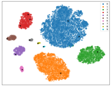
Figure 4: Visualization of the partial gradients used in RBC on CIFAR-10 with imbalance factor 200 and the corresponding cluster centroids identified by the weighted K-means clustering algorithm.

Appendix E Limitations of our work

Most of the theoretical results we present hold in a general setting except some dataset-dependent assumptions (e.g., the assumption of Theorem 1). We therefore would love to explore whether those assumptions hold for general datasets or not.

Also, our empirical claims are shown on just three standard datasets for the noisy label case and two datasets for the class imbalance case. The datasets we use are MNIST, CIFAR-10, and CIFAR-100 which are benchmark image datasets, which, however, do not include the datasets from other domains. Similarly, our empirical results use a ResNet model which is a standard neural network model for vision. We leave the evaluation of our methods on other models like Transformers for future work.

We also manually introduced label noise and a class imbalance into these datasets and have not yet evaluated on a dataset which is known to contain label noise or a class imbalance. Additionally, we use two standard types of label noise in our experiments, but our method may perform differently if the distribution of noise in another dataset is significantly different from our uniform or adversarial noise.

Furthermore, the selections of meta samples or validation samples could occur in many different scenarios, e.g., general meta learning framework andrychowicz2016learning and the data valuation methods depending on a clean validation samples (see the discussion in Section “Related Work”). Therefore, it would be interesting to explore whether the techniques proposed in this paper could address the validation sample selection problem in more general set-up.

Appendix F Discussions on societal impacts

Our framework can be useful for domains in which data is commonly noisy and imbalanced. In these settings, the sample labels are usually manually cleaned. However, labelling in these domains is expensive and may suffer from the risk of getting incorrect labels. As indicated by the experiments, our methods can perform very well when the labeling budget is very small. This thus suggests that our methods can reduce the number of required perfect labels. As a consequence, more labeling effort can be spent on the few pivotal samples to get high-quality labels, rather than a large amount of low-quality labels in these domains.

plainnat reference2

References

- Andrychowicz et al. (2016) Andrychowicz, M.; Denil, M.; Gomez, S.; Hoffman, M. W.; Pfau, D.; Schaul, T.; Shillingford, B.; and De Freitas, N. 2016. Learning to learn by gradient descent by gradient descent. Advances in neural information processing systems, 29.
- Auvolat et al. (2015) Auvolat, A.; Chandar, S.; Vincent, P.; Larochelle, H.; and Bengio, Y. 2015. Clustering is efficient for approximate maximum inner product search. arXiv preprint arXiv:1507.05910.
- Bengio et al. (2009) Bengio, Y.; Louradour, J.; Collobert, R.; and Weston, J. 2009. Curriculum learning. In Proceedings of the 26th annual international conference on machine learning, 41–48.
- Chang, Learned-Miller, and McCallum (2017) Chang, H.-S.; Learned-Miller, E.; and McCallum, A. 2017. Active bias: Training more accurate neural networks by emphasizing high variance samples. Advances in Neural Information Processing Systems, 30.
- Cui et al. (2019) Cui, Y.; Jia, M.; Lin, T.-Y.; Song, Y.; and Belongie, S. 2019. Class-balanced loss based on effective number of samples. In Proceedings of the IEEE/CVF conference on computer vision and pattern recognition, 9268–9277.
- Das et al. (2021) Das, S.; Singh, A.; Chatterjee, S.; Bhattacharya, S.; and Bhattacharya, S. 2021. Finding High-Value Training Data Subset Through Differentiable Convex Programming. In Joint European Conference on Machine Learning and Knowledge Discovery in Databases, 666–681. Springer.
- Deng (2012) Deng, L. 2012. The mnist database of handwritten digit images for machine learning research [best of the web]. IEEE signal processing magazine, 29(6): 141–142.
- Dong, Gong, and Zhu (2017) Dong, Q.; Gong, S.; and Zhu, X. 2017. Class rectification hard mining for imbalanced deep learning. In Proceedings of the IEEE International Conference on Computer Vision, 1851–1860.
- Elsayed et al. (2018) Elsayed, G.; Krishnan, D.; Mobahi, H.; Regan, K.; and Bengio, S. 2018. Large margin deep networks for classification. Advances in neural information processing systems, 31.
- Ghorbani and Zou (2019) Ghorbani, A.; and Zou, J. 2019. Data shapley: Equitable valuation of data for machine learning. In International Conference on Machine Learning, 2242–2251. PMLR.
- Hajij et al. (2021) Hajij, M.; Zamzmi, G.; Ramamurthy, K. N.; and Saenz, A. G. 2021. Data-Centric AI Requires Rethinking Data Notion. arXiv preprint arXiv:2110.02491.
- Han et al. (2018) Han, B.; Yao, Q.; Yu, X.; Niu, G.; Xu, M.; Hu, W.; Tsang, I.; and Sugiyama, M. 2018. Co-teaching: Robust training of deep neural networks with extremely noisy labels. Advances in neural information processing systems, 31.
- He et al. (2016) He, K.; Zhang, X.; Ren, S.; and Sun, J. 2016. Deep residual learning for image recognition. In Proceedings of the IEEE conference on computer vision and pattern recognition, 770–778.
- Holtz, Weng, and Mishne (2021) Holtz, C.; Weng, T.-W.; and Mishne, G. 2021. Learning Sample Reweighting for Adversarial Robustness.
- Hospedales et al. (2021) Hospedales, T. M.; Antoniou, A.; Micaelli, P.; and Storkey, A. J. 2021. Meta-Learning in Neural Networks: A Survey. IEEE Transactions on Pattern Analysis and Machine Intelligence.
- Hu et al. (2019) Hu, Z.; Tan, B.; Salakhutdinov, R. R.; Mitchell, T. M.; and Xing, E. P. 2019. Learning data manipulation for augmentation and weighting. Advances in Neural Information Processing Systems, 32.
- Irvin et al. (2019) Irvin, J.; Rajpurkar, P.; Ko, M.; Yu, Y.; Ciurea-Ilcus, S.; Chute, C.; Marklund, H.; Haghgoo, B.; Ball, R.; Shpanskaya, K.; et al. 2019. Chexpert: A large chest radiograph dataset with uncertainty labels and expert comparison. In Proceedings of the AAAI conference on artificial intelligence, volume 33, 590–597.
- Jiang et al. (2018) Jiang, L.; Zhou, Z.; Leung, T.; Li, L.-J.; and Fei-Fei, L. 2018. Mentornet: Learning data-driven curriculum for very deep neural networks on corrupted labels. In International Conference on Machine Learning, 2304–2313. PMLR.
- Karimi et al. (2020) Karimi, D.; Dou, H.; Warfield, S. K.; and Gholipour, A. 2020. Deep learning with noisy labels: Exploring techniques and remedies in medical image analysis. Medical Image Analysis, 65: 101759.
- Khan et al. (2017) Khan, S. H.; Hayat, M.; Bennamoun, M.; Sohel, F. A.; and Togneri, R. 2017. Cost-sensitive learning of deep feature representations from imbalanced data. IEEE transactions on neural networks and learning systems, 29(8): 3573–3587.
- Killamsetty et al. (2021) Killamsetty, K.; Sivasubramanian, D.; Ramakrishnan, G.; and Iyer, R. 2021. Glister: Generalization based data subset selection for efficient and robust learning. In Proceedings of the AAAI Conference on Artificial Intelligence, volume 35, 8110–8118.
- Kim et al. (2021) Kim, K.; Park, D.; Kim, K. I.; and Chun, S. Y. 2021. Task-aware variational adversarial active learning. In Proceedings of the IEEE/CVF Conference on Computer Vision and Pattern Recognition, 8166–8175.
- Koh and Liang (2017) Koh, P. W.; and Liang, P. 2017. Understanding black-box predictions via influence functions. In International conference on machine learning, 1885–1894. PMLR.
- Krizhevsky, Hinton et al. (2009) Krizhevsky, A.; Hinton, G.; et al. 2009. Learning multiple layers of features from tiny images.
- Kumar, Packer, and Koller (2010) Kumar, M.; Packer, B.; and Koller, D. 2010. Self-paced learning for latent variable models. Advances in neural information processing systems, 23.
- LeCun et al. (1998) LeCun, Y.; Bottou, L.; Bengio, Y.; and Haffner, P. 1998. Gradient-based learning applied to document recognition. Proceedings of the IEEE, 86(11): 2278–2324.
- Lewis and Gale (1994) Lewis, D. D.; and Gale, W. A. 1994. A sequential algorithm for training text classifiers. In SIGIR’94, 3–12. Springer.
- Li et al. (2022) Li, S.; Xia, X.; Ge, S.; and Liu, T. 2022. Selective-supervised contrastive learning with noisy labels. In Proceedings of the IEEE/CVF Conference on Computer Vision and Pattern Recognition, 316–325.
- Li et al. (2021) Li, Y.; Hu, P.; Liu, Z.; Peng, D.; Zhou, J. T.; and Peng, X. 2021. Contrastive clustering. In Proceedings of the AAAI Conference on Artificial Intelligence, volume 35, 8547–8555.
- Miranda (2021) Miranda, L. J. 2021. Towards data-centric machine learning: a short review. Ljvmiranda921. Github. Io.
- Mirzasoleiman, Bilmes, and Leskovec (2020) Mirzasoleiman, B.; Bilmes, J.; and Leskovec, J. 2020. Coresets for data-efficient training of machine learning models. In International Conference on Machine Learning, 6950–6960. PMLR.
- Polyzotis and Zaharia (2021) Polyzotis, N.; and Zaharia, M. 2021. What can Data-Centric AI Learn from Data and ML Engineering? arXiv preprint arXiv:2112.06439.
- Pruthi et al. (2020) Pruthi, G.; Liu, F.; Kale, S.; and Sundararajan, M. 2020. Estimating training data influence by tracing gradient descent. Advances in Neural Information Processing Systems, 33: 19920–19930.
- Ratner et al. (2017) Ratner, A. J.; Bach, S. H.; Ehrenberg, H. R.; and Ré, C. 2017. Snorkel: Fast training set generation for information extraction. In Proceedings of the 2017 ACM international conference on management of data, 1683–1686.
- Ren et al. (2018) Ren, M.; Zeng, W.; Yang, B.; and Urtasun, R. 2018. Learning to reweight examples for robust deep learning. In International conference on machine learning, 4334–4343. PMLR.
- Ren et al. (2021) Ren, P.; Xiao, Y.; Chang, X.; Huang, P.-Y.; Li, Z.; Gupta, B. B.; Chen, X.; and Wang, X. 2021. A survey of deep active learning. ACM Computing Surveys (CSUR), 54(9): 1–40.
- Russakovsky et al. (2015) Russakovsky, O.; Deng, J.; Su, H.; Krause, J.; Satheesh, S.; Ma, S.; Huang, Z.; Karpathy, A.; Khosla, A.; Bernstein, M.; et al. 2015. Imagenet large scale visual recognition challenge. International journal of computer vision, 115(3): 211–252.
- Shu et al. (2019) Shu, J.; Xie, Q.; Yi, L.; Zhao, Q.; Zhou, S.; Xu, Z.; and Meng, D. 2019. Meta-weight-net: Learning an explicit mapping for sample weighting. Advances in neural information processing systems, 32.
- Thrun and Pratt (2012) Thrun, S.; and Pratt, L. 2012. Learning to learn. Springer Science & Business Media.
- Van Engelen and Hoos (2020) Van Engelen, J. E.; and Hoos, H. H. 2020. A survey on semi-supervised learning. Machine Learning, 109(2): 373–440.
- Wang, Kucukelbir, and Blei (2017) Wang, Y.; Kucukelbir, A.; and Blei, D. M. 2017. Robust probabilistic modeling with bayesian data reweighting. In International Conference on Machine Learning, 3646–3655. PMLR.
- Wu, Weimer, and Davidson (2021) Wu, Y.; Weimer, J.; and Davidson, S. B. 2021. CHEF: a cheap and fast pipeline for iteratively cleaning label uncertainties. Proceedings of the VLDB Endowment, 14(11): 2410–2418.
- Yoon, Arik, and Pfister (2020) Yoon, J.; Arik, S.; and Pfister, T. 2020. Data valuation using reinforcement learning. In International Conference on Machine Learning, 10842–10851. PMLR.