Spatiotemporal factor models for functional data with application to population map forecast

Abstract

The proliferation of mobile devices has led to the collection of large amounts of population data. This situation has prompted the need to utilize this rich, multidimensional data in practical applications. In response to this trend, we have integrated functional data analysis (FDA) and factor analysis to address the challenge of predicting hourly population changes across various districts in Tokyo. Specifically, by assuming a Gaussian process, we avoided the large covariance matrix parameters of the multivariate normal distribution. In addition, the data were both time and spatially dependent between districts. To capture these characteristics, a Bayesian factor model was introduced, which modeled the time series of a small number of common factors and expressed the spatial structure through factor loading matrices. Furthermore, the factor loading matrices were made identifiable and sparse to ensure the interpretability of the model. We also proposed a Bayesian shrinkage method as a systematic approach for factor selection. Through numerical experiments and data analysis, we investigated the predictive accuracy and interpretability of our proposed method. We concluded that the flexibility of the method allows for the incorporation of additional time series features, thereby improving its accuracy.

Keywords: factor model, horseshoe prior, Markov chain Monte Carlo, population flow data, spatiotemporal data

Introduction

With the proliferation of mobile devices, an increasing amount of population data is being collected, and there is a growing demand for its use. Currently, we can quickly find out how many people are staying in Tokyo, Japan, at any given time or place. These data can be useful in a wide range of situations. For example, they can be utilized to reduce crowding and traffic congestion through transportation planning, to improve the efficiency of rideshares and delivery services, to promote consumption, and to guide evacuation and estimate casualty losses during disasters (Wang and Mu, 2018; Suzuki et al., 2013; Páez and Scott, 2004). Hence, analyzing population data is important; this study addresses this issue.

Our motivating dataset is population data collected by NTT Docomo, one of the largest mobile carriers in Japan. NTT Docomo has approximately 82 million customers (excluding corporate accounts) in Japan, and based on their operational data, the number of mobile terminals in each base station area is counted. The population of each area is then extrapolated with high accuracy using NTT Docomo’s cell phone penetration rate (See Terada et al., 2013; Oyabu et al., 2013, for more details). We will focus on the five special wards of Tokyo as our study area. A mesh is defined as a square of 500 meters, and there are approximately 400 meshes in the area. For each mesh, hourly population data was obtained for 365 days.

Our objective in this study is to predict the population of each district. We introduce key characteristics of the data that must be understood before constructing the model; the first is the spatial structure. Figure 1 illustrates the number of people at 14:00 on January 29, 2019, in each district of Tokyo. There are some districts with more people and some with fewer people, and these geographic changes are gradational. Hence the spatial correlation should be taken into account. Another critical feature is the time series structure. Consider the hourly population transition in two districts, an office and a residential area, for the week beginning Sunday, January 13, 2019, as shown in Figure 2. The red and blue points represent the flow of people in a business district and residential area, respectively. Basically, the population trends of the previous day are the same as those of the following day, but the population trend switches drastically between holidays (Sunday, Saturday, and Monday, which is a public holiday) and weekdays. This is intuitive; on weekdays, more people stay in the business area, whereas on holidays, downtown and residential areas are relatively more populated. In addition, the data presented here has the distinction of being large-scale, with dozens-dimension data collected over hundreds of days across numerous locations. This is a considerable obstacle in spatiotemporal modeling.

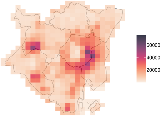
Figure 1: Number of people in central districts of Tokyo at 14:00 on January $29,2019.$

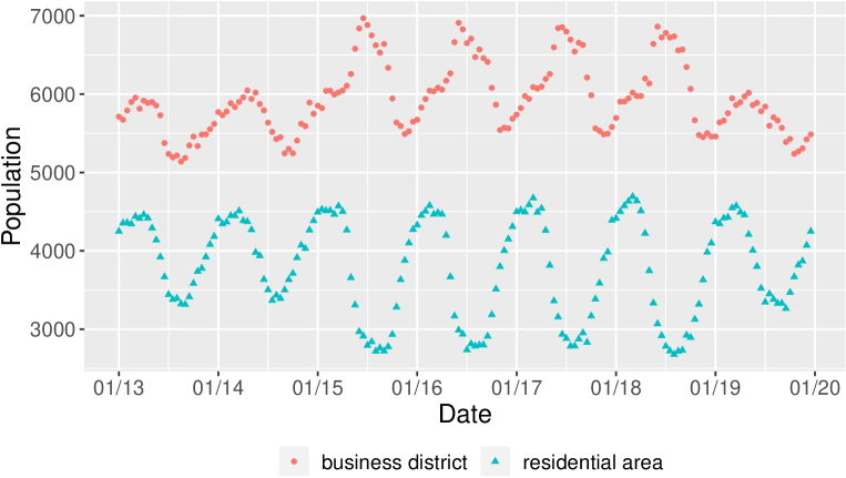
Figure 2: Hourly population data in two districts. Red represents a business district; blue represents a residential area.

To resolve those issues, we consider a novel integration of (a) functional data analysis (FDA), and (b) Bayesian factor models.

• FDA is a methodology that treats and analyzes longitudinal data as curves, reduces parameters, and facilitates the handling of high-dimensional data (Ramsay, 2004; Horváth and Kokoszka, 2012; Kokoszka and Reimherr, 2017). Even with discretely measured data, it is natural to think of the data as if there is a latent curve because the data are assumed to exist not only at the point of observation but also at other points. By assuming the path of the Gaussian process to be the underlying function, we reduce the number of parameters and analyze them.

• To efficiently estimate the mean parameters of the Gaussian process, we introduced the Bayesian factor model (e.g., Calder, 2007; Nakajima and West, 2013; Lopes, 2000, 2003). Based on the state space model, a few distinctive districts of the city are assigned as factors to reduce the computational cost because only the time series of factors needed to be considered. In addition, the factors described the temporal structure through state evolutions and the factor loading matrix captures the spatial correlation structure among districts.

These two elaborations make it possible to implement the large-scale spatiotemporal model. The method is feasible by a Gibbs sampler (Gelfand and Smith, 1990) and also allows for the development of factor selection schemes based on posterior predictive loss (PPL) (Gelfand and Ghosh, 1998). Furthermore, the factor loading matrices are set to be identifiable, and are estimated to be sparse. Identifiability, achieved by using a Cholesky-type matrix, yields unique inference results for factor loading matrices. Sparsity, made possible by newly incorporating a shrinkage prior distribution, allows us to identify which districts influence other districts. This interpretability, along with the uncertainty inherent in Bayesian models, makes predictions important in applications. Highly explanatory forecasts are effective for convincing decision-makers, and information such as 95% probability of bad case scenarios is of value to them. Since the demand for their use will continue to increase as more detailed regional and temporal population data become available, our proposed method may contribute to evidence-based policy making.

Several previous studies have addressed the FDA framework for spatio-temporal data (Zhang et al., 2023; Li et al., 2021; Wakayama and Sugasawa, 2021; Romano et al., 2011; Giraldo et al., 2011; Jiang and Serban, 2012). However, most of these have taken the approach of using time as the argument of the function and incorporating it into the analysis of spatial function data, ignoring the temporal structure. While there have been a few spatiotemporal developments in topics unrelated to forecasting (e.g., missing value completion by Zhu et al. (2022)), our contribution to the field, spatiotemporal FDA, is to propose a forecasting model that reflects spatiotemporal features in the state space. In addition, many univariate analyses of spatio-temporal data have been studied (Banerjee et al., 2003; Prado et al., 2021). Also, numerous spatio-temporal methods have also been studied for univariate data. Our method can be regarded as a generalization of these ideas to functional responses with some innovations (e.g., factor loading design), and therefore has wide applicability beyond its current use.

The remainder of the paper is organized as follows. Section 2 describes the settings, model, its computations and factor selection procedure. In Section 3, we study the features and performance of our method compared with other methods through numerical experiments. We apply our method to population flow data in Section 4. The contributions of this study are discussed in section 5.

Spatiotemporal factor models for functional data

Setting and model

Let $y_{ts}(\tau)$ be the observed functional data (population) at time $t\in\{1,\ldots,T\}$ and in region (mesh, in our application,) $s\in\{1,\ldots,N\}$ with a measurement point $\tau\in\{\tau_{1},\ldots,\tau_{K}\}$ of function. For any $t$ and $s$, we assume the following measurement error model.

$$y_{ts}(\tau) =z_{ts}(\tau)+\varepsilon_{ts},\ \ \ \ \ \varepsilon_{ts}\sim N(0,e_{s}^{2}),$$

where $\varepsilon_{ts}$ is an error term, which is independent of $t$ and $s$, $e^{2}_{s}$ is an unknown variance, and $z_{ts}$ is the focus. These models are widely adopted in the context of Bayesian modeling of functional data (Yang et al., 2016, 2017; Jiang and Serban, 2012; Wakayama and Sugasawa, 2022). Assume function $z_{ts}$ follows the Gaussian process.

$$z_{ts}(\tau)\sim\mathcal{GP}(f_{ts},\eta_{s}^{2}R(\phi_{s})),$$

where $f_{ts}$ is the mean parameter, $R(\phi_{s})=\rho_{\phi_{s}}(d)$ is correlation kernel and $\eta_{s}$ is its scale. Given the observed points, $\tau_{1},\ldots,\tau_{K}$, the above assumption leads to the following multivariate normal distribution:

$$(z_{ts}(\tau_{1}),\ldots,z_{ts}(\tau_{K}))\sim N\left((f_{ts}(\tau_{1}),\ldots,f_{ts}(\tau_{K})),\widetilde{R}_{s}\right),$$

where $\widetilde{R}_{s}$ denotes a $K\times K$ Gram matrix with $(i,j)$-components $\eta_{s}^{2}\rho_{\phi_{s}}(|\tau_{i}-\tau_{j}|)$.

Viewing a vector as a finite subset of a stochastic process is beneficial. If we attempt to estimate a $K$-dimensional covariance matrix using ordinary multivariate analysis, as many as $K\times(K-1)/2$ (e.g., $24(24-1)/2=276$ if $K=24$) parameters are required, which is laborious to estimate. However, by assuming that the vector is a finite subset of the path of a stochastic process, we only need to estimate a few parameters of the covariance kernel (only $\eta_{s}$ and $\phi_{s}$ for each point in the above case). That is, time-consuming calculations are eliminated by considering the underlying stochastic process.

State space factor models

To model the mean parameters over time and space, the following state models are considered:

$$\bm{z}_{t} =(B\otimes I_{K})\bm{x}_{t}+\bm{\nu}_{t},\ \ \ \ \ \ \bm{\nu}_{t}\sim N(\bm{0},\mathrm{blockdiag}(\widetilde{R}_{1},\ldots,\widetilde{R}_{N}))$$ (1)

$$\bm{x}_{t} =G\bm{x}_{t-1}+D_{t}\bm{\mu}+\bm{\omega}_{t},\ \ \ \ \bm{\omega}_{t}\sim N(\bm{0},\Lambda),$$

where $\bm{z}_{t}:=\left(\bm{z}_{t1},\bm{z}_{t2},\ldots,\bm{z}_{tN}\right):=\left(z_{t1}(\tau_{1}),\ldots,z_{t1}(\tau_{K}),z_{t2}(\tau_{1}),\ldots,z_{tN}(\tau_{K})\right)$ is an $NK$-dimensional vector, $\bm{x}_{t}:=\left(\bm{x}_{t1},\bm{x}_{t2},\ldots,\bm{x}_{tM}\right):=\left(x_{t1}(\tau_{1}),\ldots,x_{t1}(\tau_{K}),x_{t2}(\tau_{1}),\ldots,x_{tM}(\tau_{K})\right)$ is an $MK$-dimensional vector, $\bm{\mu}:=\left(\bm{\mu}_{1},\bm{\mu}_{2},\ldots,\bm{\mu}_{M}\right):=\left(\mu_{1}(\tau_{1}),\ldots,\mu_{M}(\tau_{K})\right)$ is an $MK$-dimensional vector, $D_{t}\in\{-1,0,1\}$ is a dummy variable, $G$ is an $MK\times MK$ state evolution matrix, $\bm{\nu}_{t}$ and $\bm{\omega}_{t}$ are the corresponding error terms, $\Lambda:=\mathrm{diag}(\lambda^{2}_{1}\ldots,\lambda_{M}^{2})$ is error variance in factor time series and $B$ is an $N\times M$-matrix denoted by

$$B =\left(\begin{array}[]{ccccc}1&0&0&\ldots&0\\ b_{21}&1&0&\ldots&0\\ b_{31}&b_{32}&1&\ldots&0\\ \vdots&\vdots&&\ddots&\vdots\\ b_{M1}&b_{M2}&b_{M3}&\ldots&1\\ b_{M+1,1}&b_{M+1,2}&b_{M+1,3}&\ldots&b_{M+1,M}\\ \vdots&\vdots&&\ddots&\vdots\\ b_{N,1}&b_{N,2}&b_{N,3}&\ldots&b_{N,M}\\ \end{array}\right).$$

Note that the number of factors $M$ is less than $N$. This formulation is a factor model (Aguilar et al., 1999; Elkhouly and Ferreira, 2021; Gamerman et al., 2008). At each $t$, a large number of vectors $\{\bm{z}_{ts}\}_{s=1}^{N}$ is represented by a small number of vectors $\{\bm{x}_{ts}\}_{s=1}^{M}$. This makes it compatible with large-scale data because only a small number of evolutions must be considered.

Furthermore, defining the factor loading matrix in this way guarantees identifiability and interpretability. Analysis might be easier if all components were parameters, but there could be multiple expressions describing the relationship between explanatory factors and explained variables, which would render the parameters inexplicable. In this case, for example, the first factor $\bm{x}_{t1}$ is equal to the first mean parameter $\bm{z}_{t1}$ minus noise; the second factor $\bm{x}_{t2}$ is equal to the second mean parameter $\bm{z}_{t2}$ minus $b_{21}\times\bm{x}_{t1}$ minus noise, and so on. That is, the $s$th factor represents the part of the $s$th trend that is not explained by the first $s-1$th factors. Hence, we formulated this method to clarify the role of each parameter.

Note that the time series equation contains the $D_{t}\bm{\mu}$ term, where $D_{t}$ depends on a combination of $t$ and $t-1$. $D_{t}$ is $1$ when $(t,t-1)$ is (holiday, weekday), $-1$ for (weekday, holiday), and $0$ otherwise. $\mu_{s}$ represents the difference in holidays compared with weekdays at each location, which allows for the modeling of day-off effects. This term can be designed more flexibly based on empirical knowledge. For example, the day before a holiday, such as Friday, tends to have a different population trend from that on a typical weekday; hence, a term can be added to reflect this:

$$\bm{z}_{t} =(B\otimes I_{K})\bm{x}_{t}+\bm{\nu}_{t},\ \ \ \ \ \ \bm{\nu}_{t}\sim N(\bm{0},\mathrm{blockdiag}(\widetilde{R}_{1},\ldots,\widetilde{R}_{N})),$$ (2)

$$\bm{x}_{t} =G\bm{x}_{t-1}+D_{t}\bm{\mu}+D_{t}^{\prime}\bm{\mu}^{\prime}+\bm{\omega}_{t},\ \ \ \ \bm{\omega}_{t}\sim N(\bm{0},\Lambda),$$

where $D_{t}^{\prime}$ and $\bm{\mu}^{\prime}$ are analogous of $D_{t}^{\prime}$ and $\bm{\mu}^{\prime}$, respectively. The benefits of this flexibility are discussed in Section 5.

Factor loading matrix

To reflect the spatial structure, we consider the column vector $\bm{b}_{\cdot s}:=(b_{s+1,s},\ldots,b_{N,s})$ of $B$ and set the following prior:

$$\bm{b}_{\cdot s}|\upsilon\theta_{s}\sim\mathcal{N}(\bm{0},\upsilon\theta_{s}^{2}Q_{s}^{-1}(\psi)),\ \ \ \ \ \ s=1,\ldots,M$$ (3)

where $\upsilon$ and $\theta_{s}$ are scale parameters, $Q_{s}(\psi)=(I-\psi W_{s})(I-\psi W_{s})^{\top}$, $\psi$ is a spatial autoregression parameter and $W_{s}$ is the adjacency matrix for $s+1$ to $N$th points, whose $(i,j)$-entry is one if district $i$ and district $j$ are adjacent and zero otherwise. This formulation is known as the CAR model (Banerjee et al., 2003), which is designed such that adjacent districts are similarly affected by a factor in this context. The $\psi$ represents their similarity. For example, if $\psi$ is $0$, then elements of $\bm{b}_{\cdot s}$ are independent and, consequently, exhibit a low similarity.

The covariance matrix of $\bm{b}_{\cdot s}$ (the effect of the $s$th factor) relies on $Q_{s}$. In other words, adjacent districts tend to be similarly affected. Additionally, designing $Q_{s}$ as a sparse matrix makes computation less expensive because fast inverse matrix computation techniques as well as fast random sampling from a multivariate normal distribution are developed (e.g., “sparseMVN” package in R language).

To facilitate the interpretability of the dependencies between districts and factors, we adopt the following prior distribution as the scale parameters:

$$\upsilon\sim C^{+}(0,1),\ \ \ \ \theta_{s}\sim C^{+}(0,1),\ \ \ s=1,...,M,$$

where $C^{+}$ denotes the half-Cauchy prior. Such prior is used in the horseshoe prior (Carvalho et al., 2009, 2010) for a univariate parameter, and the resulting distribution of $\bm{b}_{\cdot s}$ is a multivariate version of the horseshoe prior. A similar multivariate prior is adopted in Shin et al. (2020) and Wakayama and Sugasawa (2022) in non-spatial settings. The horseshoe distribution is known for its strong shrinking ability, which allows the coefficients of singular factors to be zero. In addition, unlike the Laplace distribution, it has a property called tail robustness, which firmly leaves the non-shrinking parts large. This clarifies whether the factor is effective and also allows for highlighting important venues or specific facilities.

Posterior computation

For the variance parameters, $e_{s}^{2}\sim IG(\frac{n_{e}}{2},\frac{n_{e}s_{e}}{2})$, $\lambda^{2}_{s}\sim IG(\frac{n_{\lambda}}{2},\frac{n_{\lambda}s_{\lambda}}{2})$, $\eta^{2}\sim IG(\frac{n_{\eta}}{2},\frac{n_{\eta}s_{\eta}}{2})$ are employed as an analytically tractable conjugate priors. As for the correlation kernel parameter of the Gaussian process, we set $\phi\sim IG(2,\beta)$, where $\beta=\frac{K-1}{-2\log 0.05}$ as Gamerman et al. (2008) did. Concerning the day-off effect, we assume $\mu_{s}\sim N(0,\eta_{s}^{\prime}R(\phi_{s}^{\prime})).$ To ensure evolution is a stationary process, we assume $\gamma_{s}\sim N_{tr(-1,1)}(m_{\gamma},\sigma^{2}_{\gamma})$, where $G=\mathop{\rm diag}\nolimits(\gamma_{1},\ldots,\gamma_{M})\otimes I_{K}$. We set $\psi\sim Be(1,1)$ after row normalization of each $W_{s}$. The data augmentation technique developed by Makalic and Schmidt (2015) allows the horseshoe distribution introduced in $\bm{b}_{\cdot s}$ to be re-expressed as a simple hierarchical prior. This representation also ensures that the prior conjugates and simplifies the computation of the posterior distribution.

The joint posterior density of all parameters is given by

$$\prod_{t,s,k}\pi\left(y_{ts}(\tau_{k})\mid z_{ts}(\tau_{k}),e^{2}_{s}\right)\prod_{t}\pi\left(\bm{z}_{t}\mid B,\bm{x}_{t},\bm{\eta},\bm{\phi}\right)\pi(\bm{x}_{t}\mid G,\bm{\mu},\bm{x}_{t-1},\Lambda)$$

$$\times\pi(B\mid\bm{\theta},\psi)\pi(G,\bm{e},\bm{\theta},\psi,\bm{\eta},\bm{\phi},\bm{\mu},\Lambda).$$

The full conditional distributions of all parameters, except for the Gaussian process parameters, were obtained explicitly; therefore, we implemented the Metropolis algorithm within the Gibbs sampler. The concrete posterior distribution is described below.

First, the expression for $B$ introduced in (3) is complicated; therefore, we reorganize it with respect to $\bm{b}_{\cdot s}$. Define $\widetilde{\bm{z}}_{t}^{(s)}:=(\widetilde{\bm{z}}_{t,s+1}^{(s)\top},\ldots,\widetilde{\bm{z}}_{tN}^{(s)\top})^{\top}$ where $\widetilde{\bm{z}}_{tj}^{(s)}:=\bm{z}_{tj}-\sum_{i\neq s}b_{ji}\bm{x}_{ti}$ for each $s\in\{1,...,M\}$

$$X_{ts}:=\left(\begin{array}[]{c}\bm{\iota}_{1}\otimes\bm{x}_{ts}\\ \bm{\iota}_{2}\otimes\bm{x}_{ts}\\ \vdots\\ \bm{\iota}_{N-s}\otimes\bm{x}_{ts}\end{array}\right),\ \ \ \mathrm{and}\ \ \ \bm{\iota}_{j}:=\underset{\ \widehat{j}}{(0,\ldots,0,1,0\ldots,0)}\in\mathbb{R}^{N-s}.$$

Then, we obtain $\widetilde{\bm{z}}_{t}^{(s)}=X_{ts}\bm{b}_{\cdot s}+\bm{\nu}_{t}$. Once the standard form of the regression using $\bm{b}_{\cdot s}$ is obtained, the remainder of the calculation is simple. Here, we present the full conditional distribution.

• (Sampling from $\bm{z}_{t}$)   The full conditional distribution of $\bm{z}_{t}$ is $N(\bm{m}_{z_{t}},\Sigma_{z_{t}})$, where

  $$\bm{m}_{z_{t}} =\Sigma_{z_{t}}\left(E^{-1}\bm{y}_{t}+\mathrm{blockdiag}(\widetilde{R}_{1}^{-1},...,\widetilde{R}_{N}^{-1})(B\otimes I_{K})\bm{x}_{t}\right),\ \ \$$

  $$\Sigma_{z_{t}} =\left(E^{-1}+\mathrm{blockdiag}(\widetilde{R}_{1}^{-1},...,\widetilde{R}_{N}^{-1})\right)^{-1},\ \ \$$

  $$E =\mathop{\rm diag}\nolimits(e_{s}^{2})\otimes I_{K}.$$

• (Sampling from $\bm{x}_{t}$)   The full conditional distribution of $\bm{x}_{t}$ is $N(\bm{m}_{x_{t}},\Sigma_{x_{t}})$, where

  $$\Sigma_{x_{t}} =\left((B\otimes I_{K})^{\top}\mathrm{blockdiag}(\widetilde{R}_{1}^{-1},...,\widetilde{R}_{N}^{-1})(B\otimes I_{K})+\Lambda^{-1}+G^{\top}\Lambda^{-1}G\right)^{-1},$$

  $$\bm{m}_{x_{t}} =\Sigma_{x_{t}}\Big{(}(B\otimes I_{K})^{\top}\mathrm{blockdiag}(\widetilde{R}_{1}^{-1},...,\widetilde{R}_{N}^{-1})\bm{z}_{t}+\Lambda^{-1}G\bm{x}_{t-1}$$

  $$\ \ \ \ \ \ \ \ \ \ \ \ \ +G\Lambda^{-1}\bm{x}_{t+1}+D_{t}\Lambda^{-1}\bm{\mu}-D_{t+1}G^{\top}\Lambda^{-1}\bm{\mu}\Big{)}.$$

• (Sampling from $G$)    The full conditional distribution of $\gamma_{s}$ is $N_{tr(-1,1)}(\widetilde{m}_{\gamma},\widetilde{\sigma}^{2}_{\gamma})$, where

  $$\widetilde{m}_{\gamma} =\widetilde{\sigma}^{2}_{\gamma}\left(\sum_{t=2}^{T}\frac{(\bm{x}_{ts}-D_{t}\bm{\mu}_{s})^{\top}\bm{x}_{t-1,s}}{\lambda^{2}_{s}}+\frac{m_{\gamma}}{\sigma^{2}_{\gamma}}\right),$$

  $$\widetilde{\sigma}^{2}_{\gamma} =\left(\sum_{t=2}^{T}\frac{\bm{x}_{t-1,s}^{\top}\bm{x}_{t-1,s}}{\lambda^{2}_{s}}+\frac{1}{\sigma^{2}_{\gamma}}\right)^{-1}.$$

• (Sampling from $e_{s}^{2}$)   The full conditional distribution of $e^{2}_{s}$ is

  $$IG\left(\frac{n_{e}+TK}{2},\frac{n_{e}s_{e}+\sum_{t=1}^{T}\|\bm{y}_{ts}-\bm{z}_{ts}\|_{2}^{2}}{2}\right).$$

• (Sampling from $\lambda^{2}_{s}$)   The full conditional distribution of ${\lambda}^{2}_{s}$ is

  $$IG\left(\frac{n_{\lambda}+(T-1)K}{2},\frac{n_{\lambda}s_{\lambda}+\sum_{t=2}^{T}\|\bm{x}_{ts}-\gamma_{s}\bm{x}_{t-1,s}-D_{t}\bm{\mu}_{s}\|_{2}^{2}}{2}\right).$$

• (Sampling from $\eta_{s}^{2}$)   The full conditional distribution of $\eta_{s}^{2}$ is

  $$IG\left(\frac{n_{\eta}+TK}{2},\frac{n_{\eta}s_{\eta}+\eta_{s}^{2}\sum_{t=1}^{T}(\bm{z}_{ts}-(\bm{b}_{s\cdot}\otimes I_{K})\bm{x}_{t})^{\top}\widetilde{R}^{-1}_{\phi_{s}}(\bm{z}_{ts}-(\bm{b}_{s\cdot}\otimes I_{K})\bm{x}_{t})}{2}\right).$$

• (Sampling from $\phi_{s}$)   The full conditional distribution of $\phi_{s}$ is not written in analytic form. Hence we sample $\phi_{s}$ using the random-walk Metropolis-Hastings method with acceptance rate

  $$\min\left[1,\frac{\widetilde{\phi}_{s}^{-3}\exp\left(-\frac{\beta}{\widetilde{\phi}_{s}}\right)\prod_{s}\det(\widetilde{R}_{\widetilde{\phi}_{s}})^{-\frac{1}{2}}\exp\left\{-\frac{1}{2}\left(\bm{z}_{ts}-(\bm{b}_{s\cdot}\otimes I_{K})\bm{x}_{t}\right)^{\top}\widetilde{R}_{\widetilde{\phi}_{s}}^{-1}\left(\bm{z}_{ts}-(\bm{b}_{s\cdot}\otimes I_{K})\bm{x}_{t}\right)\right\}}{\phi_{s}^{-3}\exp\left(-\frac{\beta}{\phi_{s}}\right)\prod_{s}\det(\widetilde{R}_{\phi_{s}})^{-\frac{1}{2}}\exp\left\{-\frac{1}{2}\left(\bm{z}_{ts}-(\bm{b}_{s\cdot}\otimes I_{K})\bm{x}_{t}\right)^{\top}\widetilde{R}_{\phi_{s}}^{-1}\left(\bm{z}_{ts}-(\bm{b}_{s\cdot}\otimes I_{K})\bm{x}_{t}\right)\right\}}\right].$$

• (Sampling from $\bm{\mu}_{s}$)    The full conditional distribution of $\bm{\mu}_{s}$ is $N(\bm{m}_{\mu_{s}},\Sigma_{\mu_{s}})$, where

  $$\bm{m}_{\mu_{s}} =\Sigma_{\mu_{s}}\lambda_{s}^{-2}\sum_{t=2}^{T}D_{t}(\bm{x}_{t}-G\bm{x}_{t-1}),$$

  $$\Sigma_{\mu_{s}} =\left(\sum_{t=2}^{T}D_{t}^{2}\lambda_{s}^{-1}\right)^{-1}.$$

• (Sampling from $B$) The full conditional distribution of $\bm{b}_{\cdot s}$ is $N(\bm{m}_{b},\Sigma_{b}),$ where

  $$\bm{m}_{b} =\Sigma_{b}\sum_{t=1}^{T}X_{ts}^{\top}\mathrm{blockdiag}(\widetilde{R}_{1}^{-1},...,\widetilde{R}_{N}^{-1})\widetilde{\bm{z}_{t}}^{(s)}$$

  $$\Sigma_{b} =\left(\upsilon^{2}\bm{\theta}_{s}^{-2}Q_{s}+\sum_{t=1}^{T}X_{ts}^{\top}\mathrm{blockdiag}(\widetilde{R}_{1}^{-1},...,\widetilde{R}_{N}^{-1})X_{ts}\right)^{-1}.$$

• (Sampling from $\theta_{s}^{2}$)   The full conditional distribution of ${\theta}_{s}^{2}$ is

  $$IG\left(\frac{N-s+1}{2},\frac{\bm{b}_{\cdot s}^{\top}Q_{s}(\psi)\bm{b}_{\cdot s}}{2\upsilon^{2}}+\frac{1}{\zeta_{s}}\right).$$

• (Sampling from $\zeta_{s}$)   The full conditional distribution of ${\zeta}_{s}$ is

  $$IG\left(1,\frac{1}{\theta_{s}^{2}}+1\right).$$

• (Sampling from $\upsilon^{2}$)   The full conditional distribution of $\upsilon^{2}$ is

  $$IG\left(\frac{1+\sum_{s=1}^{M}N-s}{2},\sum_{s=1}^{M}\frac{\bm{b}_{\cdot s}^{\top}Q_{s}(\psi)\bm{b}_{\cdot s}}{2\theta_{s}^{2}}+\frac{1}{\nu}\right).$$

• (Sampling from $\nu$)   The full conditional distribution of $\nu$ is

  $$IG\left(1,\frac{1}{\upsilon^{2}}+1\right).$$

• (Sampling from $\psi$)   The full conditional distribution of $\psi$ is not analytically available. Hence we implement random-walk Metropolis-Hastings with acceptance rate

  $$\min\left[1,\frac{\widetilde{\psi}^{17}(1-\widetilde{\psi})\prod_{s=1}^{M}\det\left(Q_{s}^{-1}(\widetilde{\psi})\right)^{-\frac{1}{2}}\exp\left(-\frac{\bm{b}_{\cdot s}^{\top}Q_{s}(\widetilde{\psi})\bm{b}_{\cdot s}}{2\upsilon^{2}\theta_{s}^{2}}\right)}{\psi^{17}(1-\psi)\prod_{s=1}^{M}\det\left(Q_{s}^{-1}(\psi)\right)^{-\frac{1}{2}}\exp\left(-\frac{\bm{b}_{\cdot s}^{\top}Q_{s}(\psi)\bm{b}_{\cdot s}}{2\upsilon^{2}\theta_{s}^{2}}\right)}\right].$$

Selecting factors

The critical concern in this section is how to determine the factors. Even in univariate problems, determining the factors and number of factors is difficult. The typical method is to align those that appear important based on domain knowledge (Prado et al., 2021). However, this method requires a subjective selection of factors, and it is unclear whether the selected factors are crucial. We offer the following solution to this problem.

• Prepare some factor sets as candidates.

• Assign shrinkage priors to $\upsilon$ and $\theta_{s}$ and implement the proposed method (for smaller scale data) for all candidates.

• Calculate the PPLs and choose the best factor set from the candidates.

  $${\rm PPL}=\sum_{s=1}^{N}\Biggl{[}\sum_{t=1}^{T}\left\{\bm{y}_{ts}-{\rm E}_{p}[\bm{z}_{ts}]\right\}^{\top}\left\{\bm{y}_{ts}-{\rm E}_{p}[\bm{z}_{ts}]\right\}+TK{\rm E}_{p}[\sigma_{s}^{2}]+\sum_{t=1}^{T}\mathrm{tr}\left({\rm Cov}_{p}(\bm{z}_{ts})\right)\Biggr{]}$$

• In the chosen set, if the coefficient of the $s$th factor $\bm{b}_{\cdot s}$ is unshrunk, we consider the $s$th factor necessary but delete it otherwise.

Because $\bm{b}_{\cdot s}$ is the coefficient corresponding to the $s$th factor, the $s$th factor does not affect the others (i.e., it is insignificant) if it is reduced to zero by the shrinkage distribution. Thus, we assign more factors to the model beforehand, and retain the essential factors and eliminate unnecessary factors using the effect of the shrinkage distribution.

Although this procedure allows for factor selection, implementing it on a large-scale dataset is time-consuming. This negates one advantage of the factor model, which is that it reduces the computational burden. Therefore, we recommend implementing factor selection for smaller-scale data and then implementing the proposed model with the selected factors for the entire dataset.

Numerical experiment

To confirm the usefulness of the proposed method, we investigated the properties of the proposed method and compared its accuracy with that of existing methods.

Experimental setting

First, we consider the structure of the city. We assume $N$ districts, $C_{1}-C_{N}$, where districts $C_{1}$ and $C_{2}$ are dominant, influencing the other districts, as shown in Figure 3. Assume that $C_{3}$ and $C_{4}$ are the next most influential districts and that they have the trends of $C_{1}$ and $C_{2}$, but also have their own trends, which spread to adjacent districts $C_{6}-C_{N}$. Note that it is unrealistic for a single district, either $C_{3}$ or $C_{4}$, to be adjacent to $N-4(>>10)$ districts; however, we ignore this for the numerical experiment.

The data-generating process is defined as follows.

$$\mathrm{-\ \ measurement\ error}$$

$$\ \ \ \ \ \ y_{ts}(\tau)\sim N(z_{ts}(\tau),e_{s}^{2})$$

$$\mathrm{-\ \ state\ variables\ from\ factors}$$

$$\ \ \ \ \ \ z_{1,s}(\tau)=x_{1,s}(\tau)+\mathcal{G}\mathcal{P}(0,R(1)/4),\ \ \ s=1,2,5$$

$$\ \ \ \ \ \ z_{1,3}=2/3x_{1,1}+x_{1,3}+\mathcal{G}\mathcal{P}(0,R(1)/4),$$

$$\ \ \ \ \ \ z_{1,4}=2/3x_{1,2}+x_{1,4}+\mathcal{G}\mathcal{P}(0,R(1)/4),$$

$$\ \ \ \ \ \ z_{1,s}=w_{1s}z_{1,3}+w_{2s}z_{1,4}+\mathcal{G}\mathcal{P}(0,R(1)/4),\ \ \ s=6,...,N,$$

$$\mathrm{-\ \ time\ series\ of\ factors}$$

$$\ \ \ \ \ \ x_{ts}(\tau)=0.8x_{t-1,s}(\tau)+N(\bm{0},I_{K}),\ \ \ s=1,...,5,$$

$$\ \ \ \ \ \ x_{1,1},...,x_{1,5}\overset{\mathrm{i.i.d.}}{\sim}\mathcal{G}\mathcal{P}(0,25R(4)),$$

where $R(\phi)$ is the radial basis function kernel defined as $R(\phi)=\exp(-\|\tau_{i}-\tau_{j}\|^{2}/\phi)$ and $e_{s}$ is the measurement error deviation. $z_{1,s}\ (s=6,...,N)$ is the mixture of $z_{1,3}$ and $z_{1,4}$, and their weights – $\bm{w}_{1}=\{w_{1s}\}_{s=6}^{N}$ and $\bm{w}_{2}=\{w_{2s}\}_{s=6}^{N}$ – are independently sampled from an $(N-5)$-variate Gaussian distribution with mean zero and a band-type covariance matrix, in which the diagonal is $1$, the $(i,i+1)$th and $(i,i-1)$th entries are $1/2$, and the other entries are $0$. The day-off effect is fixed at zero and is not discussed here, as it is the focus of the following section.

Figure 3: Diagram showing the influence of each district on the other districts.

All data were measured at $K(=24)$ points on the function over a period of $T$ days. The first $M(=5)$ districts were also considered factors. To perform the experiment on different space-time scales, we prepared $(20,50)$ and $(50,90)$ as combinations of $(N,T)$. We set the noise such that the signal-to-noise ratio (SNR) was the same for all points. That is, the noise variance was heterogeneous. Specifically, we set $e_{s}$ to $1/5$ (high SNR) and $1/2$ (low SNR) as the standard deviation of the signal in each district.

We conduct the following three methods

• FFM: our proposed functional factor model.

• NSFFM: non-sparse version of the functional factor model. The prior distribution of $B$ is constructed as

  $$\bm{b}_{\cdot s}|\theta\sim\mathcal{N}(\bm{0},\theta^{2}Q_{s}^{-1}(\psi)),\ \ \ \ \ \ \theta\sim IG(0.1,0.1),\ \ \ \ \ \ s=1,\ldots,M.$$

  This allowed us to investigate how the sparsity of factor loading matrix $B$ affects interpretability and estimation accuracy.

• BART: Bayesian additive regression trees developed by Chipman et al. (2010). The purpose of using BART is to study the accuracy of FFM estimation compared to nonparametric flexible methods; however, it is not a time-series method. BART can be applied by ignoring the spatial structure and considering a bivariate regression problem at each location (in this case, the explanatory variables were $t$ and $\tau$).

For all methods, we used $5000$ posterior draws after discarding $15000$ burn-in samples. The resulting sample medians were considered point estimates. To assess the point estimates and sampled posterior distribution, we adopted the following criteria.

• Root-mean-square error (RMSE): Difference between the posterior medians and the true values, defined as

  $$\mathrm{RMSE}=\sqrt{\frac{1}{NTK}\sum_{s=1}^{N}\sum_{t=1}^{T}\sum_{\tau=1}^{K}\bigl{(}\widehat{z}_{ts}(\tau)-z_{ts}(\tau)\bigl{)}^{2}}.$$

• Coverage probability (CP): Coverage accuracy of the credible interval, defined as

  $$\mathrm{CP}=\frac{1}{NTK}\sum_{s=1}^{N}\sum_{t=1}^{T}\sum_{\tau=1}^{K}\mathbb{I}_{\{\widehat{z}_{ts}^{97.5}(\tau)>z_{ts}(\tau)>\widehat{z}_{ts}^{2.5}(\tau)\}}.$$

Result

Table 1 lists the RMSEs and CPs for each scenario. The FFM and NSFFM performed better than BART. This is because BART is a nonparametric method that does not consider spatial or time-series structures, whereas FFM is a spatiotemporal method. Hence, the RMSE is lower and CP is higher for FFM than for BART. In addition, under all scenarios, FFM performed slightly better than NSFFM because the spatial structure was captured more accurately by completely eliminating unnecessary factors.

Table 1: Averaged values of root-mean-square error (RMSE) and coverage probability (CP) of 95$\%$ credible interval for functional factor model (FFM), non-sparse functional factor model (FSFFM), and Bayesian additive regression trees (BART).

SNR	$(N,T)$	Method		RMSE	CP(%)
low	(20,50)	FFM		0.459	96.6
		NSFFM		0.465	96.8
		BART		1.647	66.6
	(50,90)	FFM		0.321	97.8
		NSFFM		0.352	98.5
		BART		1.346	58.6
high	(20,50)	FFM		0.192	95.5
		NSFFM		0.197	97.3
		BART		1.341	63.3
	(50,90)	FFM		0.135	97.8
		NSFFM		0.149	98.8
		BART		1.194	55.5

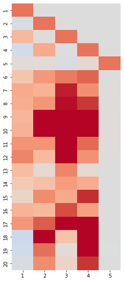
(a) FFM

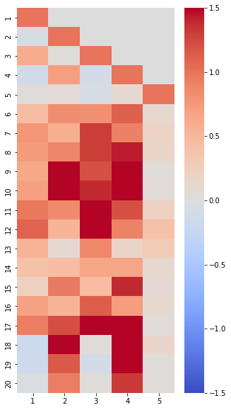
(b) NSFFM

Figure 4: Estimated factor loading matrices by functional factor model (left) and non-sparse functional factor model (right) when signal-to-noise ratio is low.

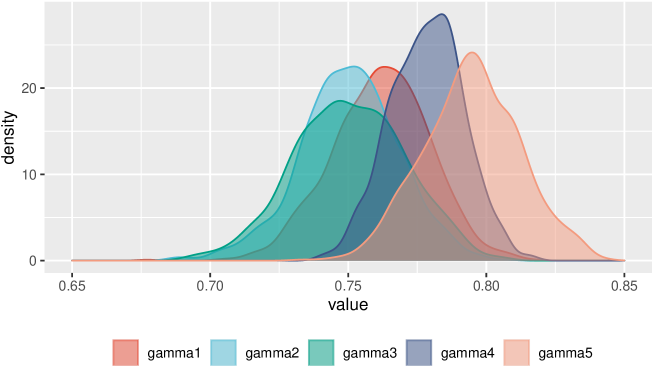
Figure 5: Posterior distribution of the autoregressive parameters.

Next, we discuss the impacts of these factors on each district. Figure 4 shows the estimated factor loading matrices, which represent the influence of five factors on twenty districts. The left plot is estimated using the FFM and the right plot is estimated using the NSFFM. The major difference between the two plots is the coefficient of the fifth factor, that is, the fifth column of matrix $B$. The NSFFM results suggest that the fifth factor has a small impact on districts 12 and 13. This is inconsistent with the original data-generating process and is misleading; because NSFFM lacks the ability to sparsify irrelevant factors, it must place some weight on these factors. By contrast, FFM removes the weights of unnecessary factors. This allowed us to clarify the connection between factors and districts.

We also considered the time-series structure. Figure 5 shows the posterior distributions of the autoregressive parameters when $(N,T)$ is $(20,50)$ and SNR is low; the results are similar for the other scenarios. All results were distributed around the true values; therefore, the time-series structure was well modeled. In particular, $\gamma_{3}$ and $\gamma_{4}$ are close to $0.8$ although they are considered challenging to estimate accurately because, unlike other factors, the 3rd and 4th factors are observed as a mixture of other factors.

Analysis of population data in Tokyo

This section describes the implementation of the proposed method using real data. Because our main aim is accurate prediction, the factors needed to be selected beforehand, the process of which is described in Section 4.1. Then, before the forecast, Section 4.2 discusses the day-off effect, which is important to understand the city. Next, the forecasting performance and possible improvements are investigated in Section 4.3. Because the data were observed hourly and daily for one year, $K=24$ and $T=365$. Saturdays, Sundays, and national holidays in 2019 were defined as days off. Because different scales at each location would make it challenging to interpret the factor loading matrix, the scale data were normalized as follows:

$$\frac{y_{ts}(\tau)}{\sqrt{\sum_{t,\tau}y_{ts}^{2}(\tau)/K/T}}.$$

Factor selection

The dataset for factor selection comprised population data for the first $100$ days and $50$ randomly selected locations.

• First, we prepared four factor sets consisting of seven elements. One set was chosen subjectively and three were chosen randomly.

• For each factor set, we implemented the proposed methods with $\upsilon\sim C^{+}(0,1),\ \theta_{s}\sim C^{+}(0,1)$, and $s=1,...,M.$

• After calculating the PPL, we chose the factor set such that the PPL was minimized. This set is listed in Table 2 and illustrated in Figure 6.

Table 2: Description of the factor districts and the explained districts.

Number	District	Description
1	Nihonbashi	Business district
2	Shibuya	Downtown
3	Sasazuka	Residential area
4	Ueno Station	Hub station
5	Shinjuku	Downtown
6	Hakusan	Residential area
7	Port of Tokyo	Seaport

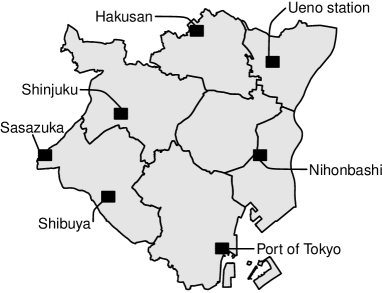
Figure 6: Locations of factor districts.

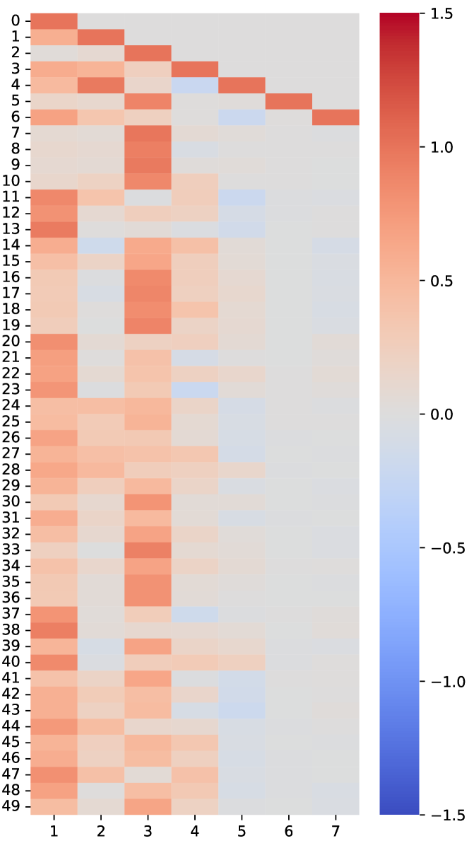
Figure 7: Estimated factor loading matrix by the proposed method.

Figure 7 shows the estimated factor loading matrix for the selected set. Several important things can be inferred from this. One is the relationship between the factors and other districts. For example, the $8-11$th and $18-20$th districts are categorized as being residential areas. In Table 2, the third factor (district) is in a residential area as well. Hence, it is natural for those districts to be well explained by the third factor. Additionally, the $12-15$th districts were office areas, similar to the first district, and the factor loading matrix was consistent with this. These relationships are intuitively plausible and allow for a more detailed understanding of the urban structure. Another noteworthy point is shrinkage. Although we selected the best factor set from the candidates in the above procedure, we could also choose factors within the set. Figure 7 exhibits that the coefficients of the sixth and seventh factors are negligible. The seventh factor was based on population data from a wharf in Tokyo, but in this case, there were no districts that could be explained by this factor. The sixth district was in a residential area which matched the third district. Hence, the trends specific to residential areas were captured by the third factor, and there was little that could be additionally explained by the sixth factor.

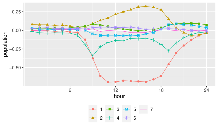
Figure 8: Day-off effects $\bm{\mu}_{s}$ of all factors.

Day-off effect

Next, we focused on the day-off effect. Figure 8 illustrates the estimated day-off effect $\bm{\mu}_{s}$ of each factor. These results provide interesting insights. The first is the day-off effect in the office districts. As represented by the first factor (the business district), there were fewer people on holidays because they did not come to work. In downtown and residential areas, the holiday population tended to increase. This is because many people went downtown to enjoy the holidays but did not leave their homes in residential areas to commute to school or work, as they did on weekdays. Another interesting feature was the day-off effect of the fourth factor. This region was a hub station and many people used it to commute to work or school. Hence, Ueno Station was particularly populated during rush hour (9:00 and 19:00) on weekdays. However, this did not occur on holidays, so that the population decreased at these times.

Prediction

Finally, we predicted future data for $400$ districts. We implemented three experiments. In the first (second, third) one, we used the first $152$ ($212$, $272$) days as training data and the following $30$ days as test data to evaluate the performance. Note that the results reported below are the average of these three experiments. Based on the discussion in Section 4.1, we employed five districts in the best set as factors. To optimize performance, we considered the following two extensions to the original method:

• Add pre-day-off effects to the factor evolution equation (2).

• Add pre-day-off effects and pre-working effects to the factor evolution equation. The latter effect was added because on weekdays before a day off there were likely to be different trends and vice versa.

To evaluate the prediction error, we define the scale-adjusted RMSE (SRMSE) as follows:

$$\frac{\sqrt{T^{-1}\sum_{t}\|\widehat{\bm{y}}_{ts}-\bm{y}_{ts}\|_{2}^{2}}}{\sqrt{T^{-1}\sum_{t}\|\bm{y}_{ts}\|_{2}^{2}}}.$$

We applied the proposed methods to train the data and obtained $5000$ posterior samples after $15000$ burn-in periods. For these samples, we obtained forecasts using the Monte Carlo approximation and reported the SRMSE values.

Table 3: Scale-adjusted root mean square error (SRMSE) of three methods for each factor, average SRMSE for non-factors, and average SRMSE for all districts on weekdays, holidays, and the entire period.

	Factor	Original FFM	Extension I	Extension II
	1	0.050	0.053	0.045
	2	0.258	0.161	0.134
All days	3	0.041	0.037	0.028
	4	0.112	0.097	0.087
	5	0.306	0.206	0.190
	Average	0.088	0.066	0.062
	1	0.039	0.041	0.041
	2	0.200	0.089	0.096
Working days	3	0.038	0.050	0.027
	4	0.110	0.089	0.070
	5	0.200	0.144	0.127
	Average	0.079	0.058	0.058
	1	0.202	0.045	0.041
	2	0.352	0.145	0.075
Days off	3	0.044	0.044	0.033
	4	0.120	0.093	0.091
	5	0.435	0.198	0.128
	Average	0.134	0.062	0.056

Table 3 shows the SRMSE of the three methods for the five factors, the average RMSEs for the non-factors, and the average RMSEs for all districts. We further divided the results into errors on weekdays and holidays and overall errors. Generally, the prediction accuracy was good, not only for the factor districts, but also for the other districts, which were represented by the aggregation of factors. This means that the factor model successfully captures the relationships among the districts. We then examined the difference between the original and extended methods. Overall, both extensions performed better than the original. By adding the pre-holiday effect, we identified the change in the shift from weekdays to holidays. This increased the precision of the estimates for both weekday and holiday trends. Focusing on changes by region, we found large declines, particularly in Districts 2 and 5, because the extensions were able to reflect the trend that people were more likely to congregate in downtown areas on Friday nights. Next, we focused on how Extension I differs from Extension II. In terms of days off, Extension II outperformed by a wide margin. The tendency to stay at home instead of going out when the following day was a working day (even on holidays) was reflected in the larger changes in downtown (Districts 2 and 5) and residential areas (District 3). Figure 9 shows the population map at 5:00, 12:00 and 19:00 on the first Monday and Sunday after 152 days. This visualizes the result that the proposed method successfully captures the difference between holidays and weekdays.

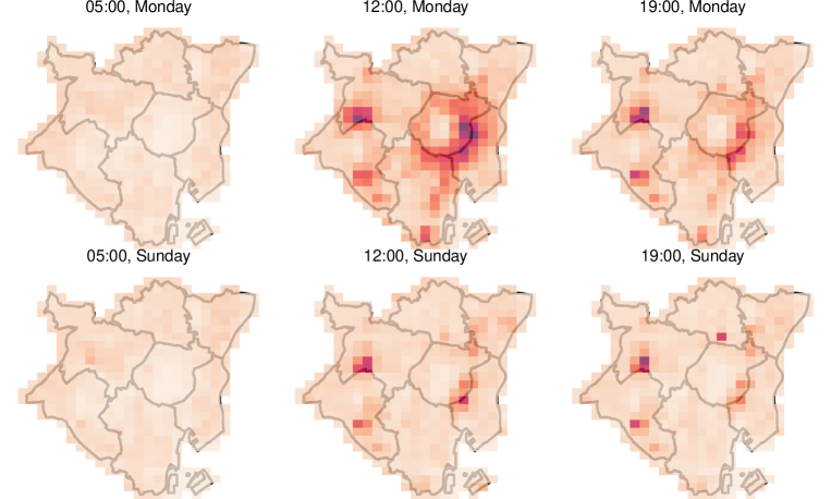
Figure 9: Predicted population map by Extension II at 05:00, 12:00 and 19:00 on Monday and Sunday.

Conclusion

In this study, a method for modeling and predicting spatiotemporal functional data was developed, with the primary application being population flow data. The immensity of the population data observed daily in each region posed a serious challenge for estimation and forecasting without increasing computational complexity and loss of interpretability. Our contribution lies in resolving these two problems. First, the integration of functional data analysis and factor models (considering the time series of a small number of state variables) allows for the computation of large data sets, and we demonstrated that the proposed method can accurately estimate and predict trends and day-off effects through simulation studies and empirical applications. Second, setting the factor loading matrix in the Cholesky-type matrix and considering spatial correlations and shrinkage effects in the column vectors provide a detailed and interpretable representation of the spatial structure, which is a key novelty of our work. Furthermore, in terms of extensions to the proposed model, we discussed that additional incorporation of domain knowledge can improve the prediction. The interpretation of the corresponding terms was simple, and further information could be extracted. Therefore, our method can facilitate the use of population data by government agencies and businesses in various areas, such as disaster prevention planning, tourism analysis, and outdoor advertising. Considering that as more people have devices, it will become possible to collect accurate data in finer meshes (that is, in more locations). Future studies should seek to develop approximate Bayesian methods to further reduce computational complexity. The source code for the proposed methods is available at the GitHub repository (https://github.com/TomWaka).

References

- Aguilar et al. (1999) Aguilar, O., R. Prado, G. Huerta, and M. West (1999). Bayesian inference on latent structure in time series (with discussion). In Bayesian Statistics 6, pp. 3–26. Oxford University Press.
- Banerjee et al. (2003) Banerjee, S., B. Carlin, A. Gelfand, J. Bernardo, M. Bayarri, J. Berger, A. Dawid, D. Heckerman, A. Smith, and M. West (2003). Hierarchical multivariate car models for spatio-temporally correlated survival data (with discussion). Bayesian Statistics 7, 45–63.
- Calder (2007) Calder, C. A. (2007). Dynamic factor process convolution models for multivariate space–time data with application to air quality assessment. Environmental and Ecological Statistics 14, 229–247.
- Carvalho et al. (2009) Carvalho, C. M., N. G. Polson, and J. G. Scott (2009). Handling sparsity via the horseshoe. In Artificial Intelligence and Statistics, pp. 73–80. PMLR.
- Carvalho et al. (2010) Carvalho, C. M., N. G. Polson, and J. G. Scott (2010). The horseshoe estimator for sparse signals. Biometrika 97(2), 465–480.
- Chipman et al. (2010) Chipman, H. A., E. I. George, and R. E. McCulloch (2010). Bart: Bayesian additive regression trees. The Annals of Applied Statistics 4(1), 266–298.
- Elkhouly and Ferreira (2021) Elkhouly, M. and M. A. Ferreira (2021). Dynamic multiscale spatiotemporal models for multivariate gaussian data. Spatial Statistics 41, 100475.
- Gamerman et al. (2008) Gamerman, D., H. F. Lopes, and E. Salazar (2008). Spatial dynamic factor analysis. Bayesian Analysis 3(4), 759–792.
- Gelfand and Ghosh (1998) Gelfand, A. E. and S. K. Ghosh (1998). Model choice: a minimum posterior predictive loss approach. Biometrika 85(1), 1–11.
- Gelfand and Smith (1990) Gelfand, A. E. and A. F. Smith (1990). Sampling-based approaches to calculating marginal densities. Journal of the American statistical association 85(410), 398–409.
- Giraldo et al. (2011) Giraldo, R., P. Delicado, and J. Mateu (2011). Ordinary kriging for function-valued spatial data. Environmental and Ecological Statistics 18(3), 411–426.
- Horváth and Kokoszka (2012) Horváth, L. and P. Kokoszka (2012). Inference for functional data with applications, Volume 200. Springer Science & Business Media.
- Jiang and Serban (2012) Jiang, H. and N. Serban (2012). Clustering random curves under spatial interdependence with application to service accessibility. Technometrics 54(2), 108–119.
- Kokoszka and Reimherr (2017) Kokoszka, P. and M. Reimherr (2017). Introduction to functional data analysis. CRC press.
- Li et al. (2021) Li, Y., D. V. Nguyen, S. Banerjee, C. M. Rhee, K. Kalantar-Zadeh, E. Kürüm, and D. Şentürk (2021). Multilevel modeling of spatially nested functional data: Spatiotemporal patterns of hospitalization rates in the us dialysis population. Statistics in medicine 40(17), 3937–3952.
- Lopes (2000) Lopes, H. F. (2000). Bayesian analysis in latent factor and longitudinal models. Duke University.
- Lopes (2003) Lopes, H. F. (2003). Expected posterior priors in factor analysis. Brazilian Journal of Probability and Statistics, 91–105.
- Makalic and Schmidt (2015) Makalic, E. and D. F. Schmidt (2015). A simple sampler for the horseshoe estimator. IEEE Signal Processing Letters 23(1), 179–182.
- Nakajima and West (2013) Nakajima, J. and M. West (2013). Bayesian analysis of latent threshold dynamic models. Journal of Business & Economic Statistics 31(2), 151–164.
- Oyabu et al. (2013) Oyabu, Y., M. Terada, T. Yamaguchi, S. Iwasawa, J. Hagiwara, and D. Koizumi (2013). Evaluating reliability of mobile spatial statistics. NTT DOCOMO Technical Journal 14(3), 16–23.
- Páez and Scott (2004) Páez, A. and D. M. Scott (2004). Spatial statistics for urban analysis: A review of techniques with examples. GeoJournal 61, 53–67.
- Prado et al. (2021) Prado, R., M. A. Ferreira, and M. West (2021). Time series: Modeling, computation, and inference.
- Ramsay (2004) Ramsay, J. O. (2004). Functional data analysis. Encyclopedia of Statistical Sciences 4.
- Romano et al. (2011) Romano, E., R. Verde, and V. Cozza (2011). Clustering spatial functional data: A method based on a nonparametric variogram estimation. New perspectives in statistical modeling and data analysis, 339–346.
- Shin et al. (2020) Shin, M., A. Bhattacharya, and V. E. Johnson (2020). Functional horseshoe priors for subspace shrinkage. Journal of the American Statistical Association 115(532), 1784–1797.
- Suzuki et al. (2013) Suzuki, T., M. Yamashita, and M. Terada (2013). Using mobile spatial statistics in field of disaster prevention planning. NTT DOCOMO Technical Journal 14(3), 37–45.
- Terada et al. (2013) Terada, M., T. Nagata, and M. Kobayashi (2013). Population estimation technology for mobile spatial statistics. NTT DOCOMO Technical Journal 14(3), 10–15.
- Wakayama and Sugasawa (2021) Wakayama, T. and S. Sugasawa (2021). Trend filtering for functional data. arXiv preprint arXiv:2104.02456.
- Wakayama and Sugasawa (2022) Wakayama, T. and S. Sugasawa (2022). Functional horseshoe smoothing for functional trend estimation. Statistica Sinica, to appear.
- Wang and Mu (2018) Wang, M. and L. Mu (2018). Spatial disparities of uber accessibility: An exploratory analysis in atlanta, usa. Computers, Environment and Urban Systems 67, 169–175.
- Yang et al. (2017) Yang, J., D. D. Cox, J. S. Lee, P. Ren, and T. Choi (2017). Efficient bayesian hierarchical functional data analysis with basis function approximations using gaussian–wishart processes. Biometrics 73(4), 1082–1091.
- Yang et al. (2016) Yang, J., H. Zhu, T. Choi, and D. D. Cox (2016). Smoothing and mean–covariance estimation of functional data with a bayesian hierarchical model. Bayesian Analysis 11(3), 649–670.
- Zhang et al. (2023) Zhang, B., H. Sang, Z. T. Luo, and H. Huang (2023). Bayesian clustering of spatial functional data with application to a human mobility study during covid-19. The Annals of Applied Statistics 17(1), 583–605.
- Zhu et al. (2022) Zhu, W., Z. Zhu, and X. Dai (2022). Spatiotemporal satellite data imputation using sparse functional data analysis. The Annals of Applied Statistics 16(4), 2291–2313.