Learning Dynamical Systems by Leveraging Data from Similar Systems

Abstract

We consider the problem of learning the dynamics of a linear system when one has access to data generated by an auxiliary system that shares similar (but not identical) dynamics, in addition to data from the true system. We use a weighted least squares approach, and provide a finite sample error bound of the learned model as a function of the number of samples and various system parameters from the two systems as well as the weight assigned to the auxiliary data. We show that the auxiliary data can help to reduce the intrinsic system identification error due to noise, at the price of adding a portion of error that is due to the differences between the two system models. We further provide a data-dependent bound that is computable when some prior knowledge about the systems is available. This bound can also be used to determine the weight that should be assigned to the auxiliary data during the model training stage.

I Introduction

Building an accurate predictive model for a dynamical system is crucial in various fields, including control theory, reinforcement learning, and economics [1]. The problem of system identification seeks to learn the system model from data when modeling from first principles is not possible. While classical system identification techniques and their associated theories focused primarily on achieving asymptotic consistency [2, 3, 4], recent efforts have sought to characterize the performance of the learned model given a finite number of samples, inspired by advances in machine learning. Having a finite sample bound for the estimation error is not only of interest on its own, but also can be integrated with techniques like robust control to come up with overall performance guarantees for the closed loop system, e.g., [5, 6, 7].

The existing literature on finite sample analysis of system identification is typically either single trajectory-based or multiple trajectories-based. The single trajectory setup assumes that one has samples from a single trajectory from the system, which enables system identification in an online manner, i.e., there is no need to restart the system from an initial state. This setup has been studied extensively over the past few years and is still an ongoing research topic [8, 9, 10, 11, 12, 13]. A key challenge in the analysis is addressing the dependencies of samples from the single trajectory. The derived sample complexity results typically show how the system identification error goes to zero by increasing the number of samples used in the single trajectory. For the multiple trajectories setup, it is typically assumed that one has access to data generated from multiple independent trajectories [6, 14, 15, 16, 17]. In practice, the multiple trajectories setup has the advantage of being able to handle unstable systems, and other cases where collecting a single long trajectory is infeasible. Technically, the assumption of independence of data usually allows for more direct use of standard concentration inequalities. Consequently, the derived results typically only show that the error goes to zero by increasing the number of trajectories. The recent paper [18] carefully addresses learning dynamical systems from a mix of both dependent and independent data, i.e., learning from multiple trajectories each with a non-trivial length. The paper [18] provides sharp bounds that hold in expectation, and shows that the error goes to zero at a rate that is determined by the product of the number of trajectories and the number of samples used from these trajectories.

We note that all of the above works make the assumption that the data used for system identification are generated from the true system model that one wants to learn. However, in many cases, collecting abundant data from the true system can be costly or even infeasible. In such cases, one may want to rely on data generated from other systems that share similar dynamics. For example, for non-engineered systems like animals, one may only have a limited amount of data from the true individual animal one wants to model, due to the challenge of conducting experiments for such systems. On the other hand, it may be possible to collect data from other animals in the herd or from a reasonably good simulator. Furthermore, when the dynamics of a system changes (e.g., due to failures), one needs to decide whether to discard all of the previous data, or to leverage the old information in an appropriate way. In settings such as the ones described above, it is of great interest to understand how one can leverage the data generated from systems that share similar (but not identical) dynamics. This idea is similar to the notion of transfer learning in the machine learning community, where one wants to transfer knowledge from related tasks to a new task [19]. However, in contrast to system identification, most of the papers on transfer learning (in the context of estimation) consider learning a static mapping from a feature space to a label space [20].

Our conference paper [21] provides finite sample analysis of system identification with the help of an auxiliary system, using a weighted least squares approach, under the assumption of having access to multiple trajectories from both the true system and the auxiliary system. The paper [21] decomposes the overall system identification error into the error due to noise and the error due to model difference, and shows that the auxiliary data can help to reduce the error due to noise by introducing a portion of constant error that is due to the difference in the models between the true and auxiliary systems. However, although the algorithm in [21] uses all samples from these trajectories (different from [6], where only two data points from each trajectory are used, assuming all samples are generated from the same system), the result is conservative in characterizing the effect of the trajectory length. In particular, the error due to noise can only go to zero by increasing the number of trajectories from the two systems.

In this paper, we address the above problem. Our contributions are as follows.

• We provide a finite sample data-independent bound for learning dynamical systems by leveraging data from an auxiliary system, using a weighted least squares approach. Again, we decompose the error into a portion due to noise and a portion due to model difference. We show that the error due to noise can go to zero by increasing either the number of trajectories or the trajectory length from the two systems, or both. The analysis is more challenging than [21] as it addresses the dependencies of samples from those independent trajectories in a less conservative way. Our analysis is general in that when the error due to model difference is zero (such that we only have the error due to noise, i.e., the two systems have same system matrices), our result qualitatively matches the results in the recent paper [18], which characterizes how the expected error goes to zero with respect to the number of trajectories and the trajectory length, assuming all samples used are generated from the same system.

• We provide insights on the benefits of using data from the auxiliary system with our data-independent bound: the auxiliary system helps to reduce the intrinsic system identification error due to noise, at the price of adding a bias that is due to model difference. Further, we provide insights on general guidelines for assigning weights to the auxiliary system, when there is not enough prior knowledge about the systems.

• We also provide a data-dependent bound that is computable when some prior knowledge about the systems is available (based on a regularized weighted least squares approach). The data-dependent bound can be used in a data-driven scheme for selecting a good weight parameter that provides better performance guarantees in practice.

• We provide various experiments capturing different scenarios to validate our results and insights.

Our analysis can be applied to a variety of important settings. For example, if the system dynamics change at some point in time (e.g., due to a fault), how should one leverage data from the prior system in order to learn the dynamics of the new system? As another example, if there is abundant data available from a simulated (but imperfect) model of the true system, how should one weight that data compared to the real data from the system? Our analysis provides insights and guidance into the answers to these questions. Our paper is organized as follows. Section II introduces relevant mathematical notation and terminology. Section III formulates the system identification problem and introduces the algorithm we use. In Section IV, we present our main results and their associated proofs. Finally, we present various numerical examples in Section V to illustrate our results, and conclude in Section VI.

II Mathematical Notation and Terminology

Let $\mathbb{R}$ denote the set of real numbers. The symbol $\cup$ is used to denote the union of sets. Let $\lambda_{min}(\cdot)$ and $\lambda_{max}(\cdot)$ be the smallest and largest eigenvalues, respectively, of a symmetric matrix. The spectral radius of a given matrix is denoted as $\rho(\cdot)$. A square matrix $A$ is called strictly stable if $\rho(A)<1$, marginally stable if $\rho(A)\leq 1$, and unstable if $\rho(A)>1$. We use $\|\cdot\|$ and $\|\cdot\|_{F}$ to denote the spectral norm and Frobenius norm of a given matrix, respectively. Vectors are treated as column vectors, and the symbol ^′ is used to denote the transpose operator. We use $\operatorname{tr}(\cdot)$ to denote the trace of a given matrix. A Gaussian distributed random vector is denoted as $u\sim\mathcal{N}(\mu,\Sigma)$, where $\mu$ is the mean and $\Sigma$ is the covariance matrix. We use $I_{n}$ to denote the identity matrix with dimension $n\times n$. The symbol $\sigma(\cdot)$ is used to denote the sigma field generated by the corresponding random vectors. We use $\mathcal{S}^{n-1}$ to denote the unit sphere in $n$-dimensional space.

III Problem formulation and algorithm

Consider the following discrete time linear time-invariant (LTI) system

$$\bar{x}_{t+1}=\bar{A}\bar{x}_{t}+\bar{B}\bar{u}_{t}+\bar{w}_{t},$$ (1)

where $\bar{x}_{t}\in\mathbb{R}^{n}$, $\bar{u}_{t}\in\mathbb{R}^{p}$, $\bar{w}_{t}\in\mathbb{R}^{n}$, are the state, input, and process noise, respectively, and $\bar{A}\in\mathbb{R}^{n\times n}$ and $\bar{B}\in\mathbb{R}^{n\times p}$ are the system matrices we wish to learn from data. The input and process noise are assumed to be i.i.d Gaussian, with $\bar{u}_{t}\sim\mathcal{N}(0,\sigma_{\bar{u}}^{2}I_{p})$ and $\bar{w}_{t}\sim\mathcal{N}(0,\sigma_{\bar{w}}^{2}I_{n})$. Note that Gaussian inputs are commonly used in system identification, e.g., [6, 16]. In this paper, we also assume that both the input $\bar{u}_{t}$ and state $\bar{x}_{t}$ can be perfectly measured.

Suppose that we have access to $N_{r}$ independent experiments of system (1), in which the system restarts from an initial state $\bar{x}_{0}\sim\mathcal{N}(0,\sigma_{\bar{x}}^{2}I_{n})$, where $\sigma_{\bar{x}}>0$, and each experiment is of length $T_{r}$. We call the state-input pairs collected from each experiment a rollout (or trajectory), and denote the set of samples we have as $\{(\bar{x}^{i}_{t},\bar{u}^{i}_{t}):1\leq i\leq N_{r},0\leq t\leq T_{r}\}$, where the superscript denotes the rollout index and the subscript denotes the time index.

Let $\bar{z}^{i}_{t}=\begin{bmatrix}\bar{x}^{i^{\prime}}_{t}&\bar{u}^{i^{\prime}}_{t}\end{bmatrix}^{{}^{\prime}}\in\mathbb{R}^{n+p}$ for $t\geq 0$. For each rollout $i$, define $\bar{X}^{i}=\begin{bmatrix}\bar{x}^{i}_{1}&\cdots&\bar{x}^{i}_{T_{r}}\end{bmatrix}\in\mathbb{R}^{n\times T_{r}}$, $\bar{Z}^{i}=\begin{bmatrix}\bar{z}^{i}_{0}&\cdots&\bar{z}^{i}_{T_{r}-1}\end{bmatrix}\in\mathbb{R}^{(n+p)\times T_{r}}$, $\bar{W}^{i}=\begin{bmatrix}\bar{w}^{i}_{0}&\cdots&\bar{w}^{i}_{T_{r}-1}\end{bmatrix}\in\mathbb{R}^{n\times T_{r}}$. Further, define the batch matrices $\bar{X}=\begin{bmatrix}\bar{X}^{1}&\cdots&\bar{X}^{N_{r}}\end{bmatrix}\in\mathbb{R}^{n\times N_{r}T_{r}},\bar{Z}=\begin{bmatrix}\bar{Z}^{1}&\cdots&\bar{Z}^{N_{r}}\end{bmatrix}\in\mathbb{R}^{(n+p)\times N_{r}T_{r}},\bar{W}=\begin{bmatrix}\bar{W}^{1}&\cdots&\bar{W}^{N_{r}}\end{bmatrix}\in\mathbb{R}^{n\times N_{r}T_{r}}$. Denoting $\Theta\triangleq\begin{bmatrix}\bar{A}&\bar{B}\end{bmatrix}\in\mathbb{R}^{n\times(n+p)}$, we have

$$\bar{X}=\Theta\bar{Z}+\bar{W}.$$

Typically, one would like to solve the following optimization problem:

$$\mathop{\min}_{\tilde{\Theta}\in\mathbb{R}^{n\times(n+p)}}\|\bar{X}-\tilde{\Theta}\bar{Z}\|^{2}_{F},$$

and obtain an estimate $\Theta_{LS}\triangleq\begin{bmatrix}\bar{A}_{LS}&\bar{B}_{LS}\end{bmatrix}$, of which the analytical form is

$$\Theta_{LS}=\bar{X}\bar{Z}^{{}^{\prime}}(\bar{Z}\bar{Z}^{{}^{\prime}})^{-1},$$

under the assumption that the matrix $\bar{Z}\bar{Z}^{{}^{\prime}}$ is invertible. The quality of the recovered estimate will depend on $N_{r}$ and $T_{r}$; in particular, if both $N_{r}$ and $T_{r}$ are small, the obtained estimate could have large estimation error [6, 8].

Suppose that, in addition to samples from the true system, we also have access to samples generated from an auxiliary system that shares “similar” dynamics to system (1). In particular, consider an auxiliary discrete time linear time-invariant system

$$\hat{x}_{t+1}=\hat{A}\hat{x}_{t}+\hat{B}\hat{u}_{t}+\hat{w}_{t},$$ (2)

where $\hat{x}_{t}\in\mathbb{R}^{n}$, $\hat{u}_{t}\in\mathbb{R}^{p}$, $\hat{w}_{t}\in\mathbb{R}^{n}$ are the state, input, and process noise, respectively, and $\hat{A}\in\mathbb{R}^{n\times n}$ and $\hat{B}\in\mathbb{R}^{n\times p}$ are system matrices. Again, the input and process noise are assumed to be i.i.d Gaussian, with $\hat{u}_{t}\sim\mathcal{N}(0,\sigma_{\hat{u}}^{2}I_{p})$ and $\hat{w}_{t}\sim\mathcal{N}(0,\sigma_{\hat{w}}^{2}I_{n})$. The above dynamics can be rewritten as

$$\hat{x}_{t+1}=(\bar{A}+\delta_{A})\hat{x}_{t}+(\bar{B}+\delta_{B})\hat{u}_{t}+\hat{w}_{t},$$ (3)

where $\delta_{A}=\hat{A}-\bar{A},\delta_{B}=\hat{B}-\bar{B}$. Intuitively, the samples generated from the above system will be useful for identifying system (1) if both $\|\delta_{A}\|$ and $\|\delta_{B}\|$ are small.

Thus, suppose that we also have access to $N_{p}$ independent experiments of system (2), in which the system restarts from an initial state $\hat{x}_{0}\sim\mathcal{N}(0,\sigma_{\hat{x}}^{2})$, where $\sigma_{\hat{x}}>0$, and each experiment is of length $T_{p}$. Let $\{(\hat{x}^{i}_{t},\hat{u}^{i}_{t}):1\leq i\leq N_{p},0\leq t\leq T_{p}\}$ denote the samples from these experiments. Let $\hat{z}^{i}_{t}=\begin{bmatrix}\hat{x}^{i^{\prime}}_{t}&\hat{u}^{i^{\prime}}_{t}\end{bmatrix}^{{}^{\prime}}\in\mathbb{R}^{n+p}$ for $t\geq 0$. The matrices $\hat{X}^{i}\in\mathbb{R}^{n\times T_{p}},\hat{Z}^{i}\in\mathbb{R}^{(n+p)\times T_{p}},\hat{W}^{i}\in\mathbb{R}^{n\times T_{p}},\hat{X}\in\mathbb{R}^{n\times N_{p}T_{p}},\hat{Z}\in\mathbb{R}^{(n+p)\times N_{p}T_{p}},\hat{W}\in\mathbb{R}^{n\times N_{p}T_{p}}$ are defined similarly, using the signals $\hat{u}^{i}_{t},\hat{x}^{i}_{t},\hat{w}^{i}_{t}$ from system (2). Let $X=\begin{bmatrix}\bar{X}&\hat{X}\end{bmatrix}\in\mathbb{R}^{n\times(N_{r}T_{r}+N_{p}T_{p})},Z=\begin{bmatrix}\bar{Z}&\hat{Z}\end{bmatrix}\in\mathbb{R}^{(n+p)\times(N_{r}T_{r}+N_{p}T_{p})},W=\begin{bmatrix}\bar{W}&\hat{W}\end{bmatrix}\in\mathbb{R}^{n\times(N_{r}T_{r}+N_{p}T_{p})}$ and $\delta_{\Theta}=\begin{bmatrix}\delta_{A}&\delta_{B}\end{bmatrix}\in\mathbb{R}^{n\times(n+p)}$. Defining

$$\Delta^{i}=\begin{bmatrix}\delta_{\Theta}\hat{z}^{i}_{0}&\cdots&\delta_{\Theta}\hat{z}^{i}_{T_{p}-1}\end{bmatrix}\in\mathbb{R}^{n\times T_{p}},\\$$

for all $i\in\{1,\dots,N_{p}\}$, and denoting

$$\Delta=\begin{bmatrix}\mathbf{0}&\cdots&\mathbf{0}&\Delta^{1}&\cdots&\Delta^{N_{p}}\end{bmatrix}\in\mathbb{R}^{n\times(N_{r}T_{r}+N_{p}T_{p})},$$

where we use $\mathbf{0}$ to denote zero matrices with appropriate dimensions, we have the relationship

$$X=\Theta Z+W+\Delta.$$ (4)

Letting $q\in\mathbb{R}_{\geq 0}$ be a design parameter that specifies the relative weight assigned to samples generated from the auxiliary system (2), we can define $Q=\operatorname{diag}(I_{N_{r}T_{r}},qI_{N_{p}T_{p}})\in\mathbb{R}^{(N_{r}T_{r}+N_{p}T_{p})\times(N_{r}T_{r}+N_{p}T_{p})}$. Setting the regularization parameter $\lambda\geq 0$, we are interested in the following (regularized-) weighted least squares problem:

$$\mathop{\min}_{\tilde{\Theta}\in\mathbb{R}^{n\times(n+p)}}\{\|XQ^{\frac{1}{2}}-\tilde{\Theta}ZQ^{\frac{1}{2}}\|^{2}_{F}+\lambda\|\tilde{\Theta}\|^{2}_{F}\}.$$ (5)

The well known (regularized-) weighted least squares estimate [22] is $\Theta_{WLS}\triangleq\begin{bmatrix}\bar{A}_{WLS}&\bar{B}_{WLS}\end{bmatrix}$, which has the form

$$\Theta_{WLS}=XQZ^{\prime}(ZQZ^{\prime}+\lambda I_{n+p})^{-1},$$ (6)

when the matrix $ZQZ^{\prime}+\lambda I_{n+p}$ is invertible. Using (4), the system identification error can be expressed as

$$\|\Theta_{WLS}-\Theta\| =\|-\lambda\Theta(ZQZ^{\prime}+\lambda I_{n+p})^{-1}$$ (7)

$$+WQZ^{\prime}(ZQZ^{\prime}+\lambda I_{n+p})^{-1}$$

$$+\Delta QZ^{\prime}(ZQZ^{\prime}+\lambda I_{n+p})^{-1}\|.$$

In particular, when the regularization parameter is set to be $\lambda=0$, we recover the standard weighted least squares estimate.

The above steps are encapsulated in Algorithm 1.

Algorithm 1 System Identification Using Auxiliary Data

1:Gather $N_{r}$ rollouts (each of length $T_{r}$) of samples generated from the true system (1), where $\bar{x}_{0}^{i}\sim\mathcal{N}(0,\sigma_{\bar{x}}^{2}I_{n})$ for all $1\leq i\leq N_{r}$.

2:Gather $N_{p}$ rollouts of samples (each of length $T_{p}$) generated from the auxiliary system (2), where $\hat{x}_{0}^{i}\sim\mathcal{N}(0,\sigma_{\hat{x}}^{2}I_{n})$ for all $1\leq i\leq N_{p}$.

3:Construct the matrices $X,Q,Z$. Compute $\Theta_{WLS}=XQZ^{\prime}(ZQZ^{\prime}+\lambda I_{n+p})^{-1}$.

4:Return the first $n$ columns of $\Theta_{WLS}$ as an estimated $\bar{A}$, and the remaining columns of $\Theta_{WLS}$ as an estimated $\bar{B}$.

Remark 1.

The weight parameter $q$ specifies how much we weight the data from the auxiliary system relative to the data from the true system, and can depend on the number of samples ($N_{r},T_{r}$ and $N_{p},T_{p}$) from each of those systems or the data available to us. The specific choice of $q$ will be discussed in detail later as we present our main results.

Our result will leverage the following definition of sub-Gaussian random vectors.

Definition 1.

A real-valued random variable $w$ is called sub-Gaussian with parameter $R^{2}$ if we have

$$\forall\alpha\in\mathbb{R},\mathbb{E}[\exp(\alpha{w})]\leq\exp(\frac{\alpha^{2}R^{2}}{2}).$$

A random vector $x\in\mathbb{R}^{n}$ is called $R^{2}$ sub-Gaussian if for all unit vectors $v\in\mathcal{S}^{n-1}$ the random variable $v^{\prime}x$ is $R^{2}$ sub-Gaussian.

Note that $w\in\mathbb{R}^{n}$ is sub-Gaussian with parameter $\|\Sigma\|$ if $w$ is a Gaussian random vector with zero mean and covariance matrix $\Sigma\in\mathbb{R}^{n\times n}$.

To ease the notation, we let $\bar{\sigma}_{min}\triangleq\min(\bar{\sigma}_{x},\bar{\sigma}_{w},\bar{\sigma}_{u})$, $\hat{\sigma}_{min}\triangleq\min(\hat{\sigma}_{x},\hat{\sigma}_{w},\hat{\sigma}_{u})$, $\bar{\sigma}_{max}\triangleq\max(\bar{\sigma}_{x},\bar{\sigma}_{w},\bar{\sigma}_{u})$, and $\hat{\sigma}_{max}\triangleq\max(\hat{\sigma}_{x},\hat{\sigma}_{w},\hat{\sigma}_{u})$. Further, define the following matrices:

$$\bar{G}_{t}\triangleq\sum_{i=0}^{t}\bar{A}^{i}\bar{A}^{i}{{}^{\prime}}+\sum_{i=0}^{t-1}\bar{A}^{i}\bar{B}\bar{B}^{\prime}\bar{A}^{i}{{}^{\prime}},$$ (8)

$$\hat{G}_{t}\triangleq\sum_{i=0}^{t}\hat{A}^{i}\hat{A}^{i}{{}^{\prime}}+\sum_{i=0}^{t-1}\hat{A}^{i}\hat{B}\hat{B}^{\prime}\hat{A}^{i}{{}^{\prime}}.$$

In the next section, we provide both a data-independent bound (assuming $\lambda=0$) and a data-dependent bound (assuming $\lambda>0$) of the system identification error in (7). We study the case when $\lambda=0$ in the data-independent bound to highlight our key insights (the benefits of the auxiliary data and the role of the weight parameter $q$), and the result for $\lambda>0$ can be easily generalized. The data-independent finite sample upper bound characterizes the error as a function of $N_{r},T_{r},N_{p},T_{p},\sigma_{\bar{w}},\sigma_{\hat{w}},q,\|\delta_{\Theta}\|$ and other parameters from the true system and the auxiliary system. While the data-independent error bound provides insights on the benefits of using the auxiliary samples, the derived result may not be used directly in practice, since it involves unknown system parameters. To address that, we also provide a data-dependent bound for the case when $\lambda>0$. The non-zero regularization parameter $\lambda$ not only helps us to derive the data-dependent result, but also provides the user with more flexibility to tune the estimate in practice. The derived data-dependent bound is computable, applicable to more general input and noise, and can be used in real-world applications to select the weight parameter $q$ (and regularization parameter $\lambda$). More specifically, the bound characterizes the error as a function of $\sigma_{\bar{w}},\sigma_{\hat{w}},q,\|\delta_{\Theta}\|$, $\lambda$, $\|\Theta\|$, and the available data. Both our data-independent bound and data-dependent bound will provide insights and guidance on selecting an appropriate weight parameter $q$. We will assume that system (1) and system (2) have the same stability in our discussions, i.e., both $\rho(\bar{A})$ and $\rho(\hat{A})$ are less than 1, or both $\rho(\bar{A})$ and $\rho(\hat{A})$ are equal to 1, or both $\rho(\bar{A})$ and $\rho(\hat{A})$ are greater than 1 (although $\rho(\bar{A})$ does not need to equal to $\rho(\hat{A})$), but similar insights can be extended even if they are different.

IV Analysis of the System Identification Error

In this section, we derive both a data-independent bound (assuming $\lambda=0$) and a data-dependent bound (assuming $\lambda>0$) on the system identification error in (7). The proof of the data-independent bound follows by upper bounding the error terms $\|WQZ^{\prime}(ZQZ^{\prime})^{-\frac{1}{2}}\|$, $\|(ZQZ^{\prime})^{-\frac{1}{2}}\|$, and $\|\Delta QZ^{\prime}\|$ separately. The proof of the data-dependent bound follows by directly evaluating an upper bound of the term (7) from data, but with the replacement of the noise-dependent term $\|WQZ^{\prime}(ZQZ^{\prime}+\lambda I_{n+p})^{-\frac{1}{2}}\|$ by a high-probability upper bound. We will start with some intermediate results pertaining to these quantities.

IV-A Intermediate Results

We will use the following result to establish a lower bound for the smallest eigenvalue of the matrix $ZQZ^{\prime}$.

Lemma 1.

[23, Lemma 36] Let $\{z_{t}\}_{t\geq 0}$ be a sequence of random vectors that is adapted to a filtration $\{\mathcal{F}_{t}\}_{t\geq 0}$, where $z_{t}\in\mathbb{R}^{d}$ for all $t\geq 0$. Suppose $z_{t}$ is conditionally Gaussian on $\mathcal{F}_{t-1}$ with $\mathbb{E}[z_{t}z_{t}^{\prime}|\mathcal{F}_{t-1}]\succeq\sigma_{z}^{2}I_{d}$ for all $t\geq 1$, where $\sigma_{z}>0$. Then, for any fixed $\delta>0$ and any $T\geq 200d\log(\frac{12}{\delta})$, the following inequality holds with probability at least $1-\delta$:

$$\sum_{t=0}^{T-1}z_{t}z_{t}^{\prime}\succeq\frac{(T-1)\sigma_{z}^{2}}{40}I_{d}.$$

We have the following result.

Proposition 1.

Fixing $\delta>0$, when $\min(N_{r}T_{r},N_{p}T_{p})\geq\max(41,200(n+p)\log(\frac{12}{\delta}))$, we have with probability at least $1-2\delta$

$$ZQZ^{\prime}\succeq\frac{N_{r}T_{r}\bar{\sigma}_{min}^{2}+qN_{p}T_{p}\hat{\sigma}_{min}^{2}}{41}I_{n+p}.$$

Proof.

We have

$$ZQZ^{\prime} =\bar{Z}\bar{Z}^{\prime}+q\hat{Z}\hat{Z}^{\prime}=\sum_{i=1}^{N_{r}}\sum_{t=0}^{T_{r}-1}\bar{z}^{i}_{t}\bar{z}^{i^{\prime}}_{t}+q\sum_{j=1}^{N_{p}}\sum_{k=0}^{T_{p}-1}\hat{z}^{j}_{k}\hat{z}^{j^{\prime}}_{k}.$$ (9)

We now focus on the first summation in (9) since the analysis for the second one is essentially the same. We can define the sequence $\{z_{t}\}_{t\geq 0}$ as

$$z_{t}=\begin{cases}\bar{z}^{1}_{t}&\text{if}\quad 0\leq t\leq T_{r}-1\\ \bar{z}^{2}_{t-T_{r}}&\text{if}\quad T_{r}\leq t\leq 2T_{r}-1\\ \bar{z}^{3}_{t-2T_{r}}&\text{if}\quad 2T_{r}\leq t\leq 3T_{r}-1\\ \vdots&\vdots,\\ \end{cases}$$

where $\bar{z}^{a}_{b}$ for $a>N_{r}$ and $b=0,\ldots,T_{r}-1$ are generated using the same way as $\bar{z}^{a}_{b}$ for $a=1,\ldots,N_{r}$ and $b=0,\ldots,T_{r}-1$. In words, $z_{t}$ is the sequence formed by concatenating the sequence $\{z_{t}^{1}\}_{t=0}^{T_{r}-1},\{z_{t}^{2}\}_{t=0}^{T_{r}-1},\ldots$. The sequences $\{w_{t}\}_{t\geq 0}$ and $\{u_{t}\}_{t\geq 0}$ are defined similarly using the signals $\bar{w}^{i}_{t}$ and $\bar{u}^{i}_{t}$. Further, we define the sequence $\{x_{t}\}_{t\geq 0}$ as $x_{t}=\bar{x}^{t+1}_{0}$, where $\bar{x}^{a}_{0}$ for $a>N_{r}$ are generated using the same way as $\bar{x}^{a}_{0}$ for $a=1,\ldots,N_{r}$. With these definitions, we have

$$\sum_{i=1}^{N_{r}}\sum_{t=0}^{T_{r}-1}\bar{z}_{t}^{i}\bar{z}^{i^{\prime}}_{t}=\sum_{t=0}^{N_{r}T_{r}-1}z_{t}z_{t}^{\prime}.$$

Now define the filtration $\{\mathcal{F}_{t}\}_{t\geq 0}$, where $\mathcal{F}_{t}=\sigma(z_{0},z_{1},\ldots,z_{t})$ for $t\geq 0$. Note that $z_{t}|\mathcal{F}_{t-1}$ is a Gaussian random vector for $t\geq 1$. For $t$ satisfying $t\geq 1$ and $t\bmod T_{r}\neq 0$, we have

$$z_{t}|\mathcal{F}_{t-1}=\begin{bmatrix}\Theta z_{t-1}|\mathcal{F}_{t-1}\\ 0\end{bmatrix}+\begin{bmatrix}w_{t-1}\\ u_{t}\end{bmatrix},$$

from which we have

$$\mathbb{E}[z_{t}z_{t}^{\prime}|\mathcal{F}_{t-1}] \succeq\begin{bmatrix}\sigma_{\bar{w}}^{2}I_{n}&0\\ 0&\sigma_{\bar{u}}^{2}I_{p}\end{bmatrix}$$

$$\succeq\bar{\sigma}_{min}^{2}I_{n+p}.$$

For $t$ satisfying $t\geq 1$ and $t\bmod T_{r}=0$, we have

$$z_{t}|\mathcal{F}_{t-1}=\begin{bmatrix}x_{\frac{t}{T_{r}}}\\ u_{t}\end{bmatrix},$$

from which we have

$$\mathbb{E}[z_{t}z_{t}^{\prime}|\mathcal{F}_{t-1}] =\begin{bmatrix}\sigma_{\bar{x}}^{2}I_{n}&0\\ 0&\sigma_{\bar{u}}^{2}I_{p}\end{bmatrix}$$

$$\succeq\bar{\sigma}_{min}^{2}I_{n+p}.$$

Consequently, for all $t\geq 1$, we have

$$\mathbb{E}[z_{t}z_{t}^{\prime}|\mathcal{F}_{t-1}] \succeq\bar{\sigma}_{min}^{2}I_{n+p}.$$

Fixing $\delta>0$ and letting $N_{r}T_{r}\geq\max(41,200(n+p)\log(\frac{12}{\delta}))$, we can apply Lemma 1 to get

$$\sum_{i=1}^{N_{r}}\sum_{t=0}^{T_{r}-1}\bar{z}_{t}^{i}\bar{z}^{i^{\prime}}_{t}=\sum_{t=0}^{N_{r}T_{r}-1}z_{t}z_{t}^{\prime} \succeq\frac{(N_{r}T_{r}-1)\bar{\sigma}_{min}^{2}}{40}I_{n+p}$$

$$\succeq\frac{N_{r}T_{r}\bar{\sigma}_{min}^{2}}{41}I_{n+p}$$

with probability at least $1-\delta$. Applying a similar procedure for the second summation in (9) and leveraging a union bound, we have with probability at least $1-2\delta$

$$\sum_{i=1}^{N_{r}}\sum_{t=0}^{T_{r}-1}\bar{z}^{i}_{t}\bar{z}^{i^{\prime}}_{t}+q\sum_{j=1}^{N_{p}}\sum_{k=0}^{T_{p}-1}\hat{z}^{j}_{k}\hat{z}^{j^{\prime}}_{k}$$

$$\succeq\frac{N_{r}T_{r}\bar{\sigma}_{min}^{2}+qN_{p}T_{p}\hat{\sigma}_{min}^{2}}{41}I_{n+p}.$$

∎

We will leverage the following Hanson-Wright inequality to upper bound the terms $\|\bar{Z}\bar{Z}^{\prime}\|$ and $\|\hat{Z}\hat{Z}^{\prime}\|$.

Lemma 2.

[24, Theorem 1.1] Let $X=\begin{bmatrix}X_{1}&\ldots X_{n}\end{bmatrix}^{\prime}\in\mathbb{R}^{n}$ be a random vector with independent components $X_{i}$ which satisfy $\mathbb{E}[X_{i}]=0$ and $\|X_{i}\|_{\psi_{2}}\leq K$, where $\|\cdot\|_{\psi_{2}}$ denotes the sub-Gaussian norm, i.e., $\|X_{i}\|_{\psi_{2}}=\inf\{\zeta>0:\mathbb{E}[\exp(X_{i}^{2}/\zeta^{2})]\leq 2\}$. Let $A$ be an $n\times n$ matrix. Then, for every $t\geq 0$, we have

$$P(|X^{\prime}AX-\mathbb{E}[X^{\prime}AX]|>t)$$

$$\leq 2\exp(-c_{0}\min(\frac{t^{2}}{K^{4}\|A\|^{2}_{F}},\frac{t}{K^{2}\|A\|})),$$

where $c_{0}$ is some positive universal constant.

We have the following result.

Lemma 3.

For any fixed $\delta\in(0,\frac{2}{e})$, each of the following inequalities holds with probability at least $1-\delta$:

$$\|\sum_{i=1}^{N_{r}}\sum_{t=0}^{T_{r}-1}\bar{z}_{t}\bar{z}^{\prime}_{t}\|\leq N_{r}\sum_{t=0}^{T_{r}-1}(\operatorname{tr}(\bar{G}_{t})+p)(\frac{1}{c}\log(\frac{2}{\delta})+1)\bar{\sigma}_{max}^{2},$$

$$\|\sum_{i=1}^{N_{r}}\sum_{t=0}^{T_{p}-1}\hat{z}_{t}\hat{z}^{\prime}_{t}\|\leq N_{p}\sum_{t=0}^{T_{p}-1}(\operatorname{tr}(\hat{G}_{t})+p)(\frac{1}{c}\log(\frac{2}{\delta})+1)\hat{\sigma}_{max}^{2},$$

where $c$ is some positive constant.

Proof.

We will only show the first inequality since the analysis for the second one is essentially the same. Let $\mathbf{Z}_{T_{r}}^{N_{r}}=\begin{bmatrix}\mathbf{Z}^{1^{\prime}}&\ldots&\mathbf{Z}^{N_{r}^{\prime}}\end{bmatrix}^{\prime}\in\mathbb{R}^{(n+p)N_{r}T_{r}}$, where $\mathbf{Z}^{i}=\begin{bmatrix}\bar{z}_{0}^{i^{\prime}}&\ldots&\bar{z}_{T_{r}-1}^{i^{\prime}}\end{bmatrix}^{\prime}\in\mathbb{R}^{(n+p)T_{r}}$ for $i=1,\ldots,N_{r}$. We have

$$\|\sum_{i=1}^{N_{r}}\sum_{t=0}^{T_{r}-1}\bar{z}_{t}^{i}\bar{z}^{i^{\prime}}_{t}\|\leq\sum_{i=1}^{N_{r}}\sum_{t=0}^{T_{r}-1}\bar{z}_{t}^{i^{\prime}}\bar{z}_{t}^{i}=\mathbf{Z}_{T_{r}}^{N_{r}^{\prime}}\mathbf{Z}_{T_{r}}^{N_{r}}.$$ (10)

Note that we have

$$\mathbf{Z}_{T_{r}}^{N_{r}^{\prime}}\mathbf{Z}_{T_{r}}^{N_{r}} \leq\mathbb{E}[\mathbf{Z}_{T_{r}}^{N_{r}^{\prime}}\mathbf{Z}_{T_{r}}^{N_{r}}]+|\mathbf{Z}_{T_{r}}^{N_{r}^{\prime}}\mathbf{Z}_{T_{r}}^{N_{r}}-\mathbb{E}[\mathbf{Z}_{T_{r}}^{N_{r}^{\prime}}\mathbf{Z}_{T_{r}}^{N_{r}}]|.$$ (11)

Now we will upper bound the two terms after the inequality in (11). We consider the term $\mathbb{E}[\mathbf{Z}_{T_{r}}^{N_{r}^{\prime}}\mathbf{Z}_{T_{r}}^{N_{r}}]$ first. Let

$$H=\begin{bmatrix}H_{1}&H_{2}\end{bmatrix}\in\mathbb{R}^{{}^{(n+p)T_{r}\times(n+p)T_{r}}},$$

where $H_{1}\in\mathbb{R}^{(n+p)T_{r}\times nT_{r}}$ is defined as

$$H_{1}=\begin{bmatrix}I_{n}&\mathbf{0}&\mathbf{0}&\cdots&\mathbf{0}&\mathbf{0}\\ \mathbf{0}&\mathbf{0}&\mathbf{0}&\cdots&\mathbf{0}&\mathbf{0}\\ \bar{A}&I_{n}&\mathbf{0}&\cdots&\mathbf{0}&\mathbf{0}\\ \mathbf{0}&\mathbf{0}&\mathbf{0}&\cdots&\mathbf{0}&\mathbf{0}\\ \bar{A}^{2}&\bar{A}&I_{n}&\cdots&\mathbf{0}&\mathbf{0}&\\ \mathbf{0}&\mathbf{0}&\mathbf{0}&\cdots&\mathbf{0}&\mathbf{0}\\ \vdots&\vdots&\vdots&\vdots&\vdots&\vdots&\\ \bar{A}^{T_{r}-1}&\bar{A}^{T_{r}-2}&\bar{A}^{T_{r}-3}&\cdots&\bar{A}&I_{n}\\ \mathbf{0}&\mathbf{0}&\mathbf{0}&\cdots&\mathbf{0}&\mathbf{0}\\ \end{bmatrix},$$

and $H_{2}\in\mathbb{R}^{(n+p)T_{r}\times pT_{r}}$ is defined as

$$H_{2}=\begin{bmatrix}\mathbf{0}&\mathbf{0}&\mathbf{0}&\cdots&\mathbf{0}&\mathbf{0}\\ I_{p}&\mathbf{0}&\mathbf{0}&\cdots&\mathbf{0}&\mathbf{0}\\ \bar{B}&\mathbf{0}&\mathbf{0}&\cdots&\mathbf{0}&\mathbf{0}\\ \mathbf{0}&I_{p}&\mathbf{0}&\cdots&\mathbf{0}&\mathbf{0}\\ \bar{A}\bar{B}&\bar{B}&\mathbf{0}&\cdots&\mathbf{0}&\mathbf{0}&\\ \mathbf{0}&\mathbf{0}&I_{p}&\cdots&\mathbf{0}&\mathbf{0}\\ \vdots&\vdots&\vdots&\vdots&\vdots&\vdots&\\ \bar{A}^{T_{r}-2}\bar{B}&\bar{A}^{T_{r}-3}\bar{B}&\bar{A}^{T_{r}-4}\bar{B}&\cdots&\bar{B}&\mathbf{0}\\ \mathbf{0}&\mathbf{0}&\mathbf{0}&\cdots&\mathbf{0}&I_{p}\\ \end{bmatrix},$$

where we use $\mathbf{0}$ to denote zero matrices with appropriate dimensions. Further, let $\mathbf{H}=\operatorname{diag}(H,\cdots,H)\in\mathbb{R}^{(n+p)N_{r}T_{r}\times(n+p)N_{r}T_{r}}$ and $g=\begin{bmatrix}g^{1^{\prime}}&g^{2^{\prime}}&\cdots&g^{N_{r}^{\prime}}\\ \end{bmatrix}^{\prime}\in\mathbb{R}^{(n+p)N_{r}T_{r}}$, where $g^{i}=\begin{bmatrix}\bar{x}_{0}^{i^{\prime}}&\bar{w}_{0}^{i^{\prime}}&\cdots&\bar{w}_{T_{r}-2}^{i^{\prime}}&\bar{u}_{0}^{i^{\prime}}&\cdots&\bar{u}_{T_{r}-1}^{i^{\prime}}\\ \end{bmatrix}^{\prime}\in\mathbb{R}^{(n+p)T_{r}}$ for $i=1,\ldots,N_{r}$. With these definitions, we have $\mathbf{H}g=\begin{bmatrix}\mathbf{Z}^{1^{\prime}}&\ldots&\mathbf{Z}^{N_{r}^{\prime}}\end{bmatrix}^{\prime}=\mathbf{Z}_{T_{r}}^{N_{r}}$, and hence

$$\mathbf{Z}_{T_{r}}^{N_{r}^{\prime}}\mathbf{Z}_{T_{r}}^{N_{r}}=g^{\prime}\mathbf{H}^{\prime}\mathbf{H}g=\operatorname{tr}(g^{\prime}\mathbf{H}^{\prime}\mathbf{H}g)=\operatorname{tr}(gg^{\prime}\mathbf{H}^{\prime}\mathbf{H}).$$ (12)

Taking the expectation, and from the relationship $\operatorname{tr}(AB)\leq\lambda_{max}(A)\operatorname{tr}(B)$ for real symmetric $A$ and real $B\succeq 0$ [25], we have

$$\mathbb{E}[\operatorname{tr}(gg^{\prime}\mathbf{H}^{\prime}\mathbf{H})] =\operatorname{tr}(\mathbb{E}[gg^{\prime}]\mathbf{H}^{\prime}\mathbf{H})\leq\|\mathbb{E}[gg^{\prime}]\|\operatorname{tr}(\mathbf{H}^{\prime}\mathbf{H})$$ (13)

$$=\bar{\sigma}_{max}^{2}\operatorname{tr}(\mathbf{H}^{\prime}\mathbf{H})=\bar{\sigma}_{max}^{2}N_{r}\operatorname{tr}(H^{\prime}H)$$

$$=\bar{\sigma}_{max}^{2}N_{r}(\sum_{t=0}^{T_{r}-1}\operatorname{tr}(\bar{G}_{t})+\sum_{k=0}^{T_{r}-1}\operatorname{tr}(I_{p}))$$

$$=\bar{\sigma}_{max}^{2}N_{r}\sum_{t=0}^{T_{r}-1}(\operatorname{tr}(\bar{G}_{t})+p),$$

where $\bar{G}_{t}$ is defined in (8). Now we consider the term $|\mathbf{Z}_{T_{r}}^{N_{r}^{\prime}}\mathbf{Z}_{T_{r}}^{N_{r}}-\mathbb{E}[\mathbf{Z}_{T_{r}}^{N_{r}^{\prime}}\mathbf{Z}_{T_{r}}^{N_{r}}]|$ in (11). From (12), we have

$$|\mathbf{Z}_{T_{r}}^{N_{r}^{\prime}}\mathbf{Z}_{T_{r}}^{N_{r}}-\mathbb{E}[\mathbf{Z}_{T_{r}}^{N_{r}^{\prime}}\mathbf{Z}_{T_{r}}^{N_{r}}]|=|g^{\prime}\mathbf{H}^{\prime}\mathbf{H}g-\mathbb{E}[g^{\prime}\mathbf{H}^{\prime}\mathbf{H}g]|.$$

From [26], we have each component of $g$ has sub-Gaussian norm upper bounded by $\sqrt{3}\bar{\sigma}_{max}$. We can apply Lemma 2 to the above term with the replacement of $c_{0}$ by $\min(1,c_{0})$ to obtain

$$P(|g^{\prime}\mathbf{H}^{\prime}\mathbf{H}g-\mathbb{E}[g^{\prime}\mathbf{H}^{\prime}\mathbf{H}g]|>t)$$ (14)

$$\leq 2\exp(-\min(\frac{c_{0}t^{2}}{9\bar{\sigma}_{max}^{4}\|\mathbf{H}^{\prime}\mathbf{H}\|^{2}_{F}},\frac{c_{0}t}{3\bar{\sigma}_{max}^{2}\|\mathbf{H}^{\prime}\mathbf{H}\|}))$$

$$\leq 2\exp(-\min(\frac{ct^{2}}{\bar{\sigma}_{max}^{4}\|\mathbf{H}^{\prime}\mathbf{H}\|^{2}_{F}},\frac{ct}{\bar{\sigma}_{max}^{2}\|\mathbf{H}^{\prime}\mathbf{H}\|})),$$

where $c\triangleq\frac{c_{0}}{9}$.

Fixing $\delta\in(0,\frac{2}{e})$ and setting $t=\frac{1}{c}\log(\frac{2}{\delta})\bar{\sigma}_{max}^{2}\operatorname{tr}(\mathbf{H}^{\prime}\mathbf{H})$, we have

$$\frac{ct^{2}}{\bar{\sigma}_{max}^{4}\|\mathbf{H}^{\prime}\mathbf{H}\|_{F}^{2}} =\frac{1}{c}(\frac{\operatorname{tr}(\mathbf{H}^{\prime}\mathbf{H})}{\|\mathbf{H}^{\prime}\mathbf{H}\|_{F}})^{2}(\log(\frac{2}{\delta}))^{2}$$

$$\geq(\log(\frac{2}{\delta}))^{2}\geq\log(\frac{2}{\delta}),$$

and

$$\frac{ct}{\bar{\sigma}_{max}^{2}\|\mathbf{H}^{\prime}\mathbf{H}\|} =\log(\frac{2}{\delta})\frac{\operatorname{tr}(\mathbf{H}^{\prime}\mathbf{H})}{\|\mathbf{H}^{\prime}\mathbf{H}\|}\geq\log(\frac{2}{\delta}),$$

where we used the fact that $\|\mathbf{H}^{\prime}\mathbf{H}\|\leq\|\mathbf{H}^{\prime}\mathbf{H}\|_{F}\leq\|\mathbf{H}\|^{2}_{F}=\operatorname{tr}(\mathbf{H}^{\prime}\mathbf{H})$.

Combining the above inequalities with (14), we have with probability at least $1-\delta$

$$|\mathbf{Z}_{T_{r}}^{N_{r}^{\prime}}\mathbf{Z}_{T_{r}}^{N_{r}}-\mathbb{E}[\mathbf{Z}_{T_{r}}^{N_{r}^{\prime}}\mathbf{Z}_{T_{r}}^{N_{r}}]|=|g^{\prime}\mathbf{H}^{\prime}\mathbf{H}g-\mathbb{E}[g^{\prime}\mathbf{H}^{\prime}\mathbf{H}g]|$$

$$\leq\frac{1}{c}\log(\frac{2}{\delta})\bar{\sigma}_{max}^{2}\operatorname{tr}(\mathbf{H}^{\prime}\mathbf{H})$$

$$=\frac{1}{c}\log(\frac{2}{\delta})\bar{\sigma}_{max}^{2}N_{r}\sum_{t=0}^{T_{r}-1}(\operatorname{tr}(\bar{G}_{t})+p).$$

Consequently, considering the above inequality in conjunction with (13), and from (11), we have with probability at least $1-\delta$

$$\mathbf{Z}_{T_{r}}^{N_{r}^{\prime}}\mathbf{Z}_{T_{r}}^{N_{r}} \leq N_{r}\sum_{t=0}^{T_{r}-1}(\operatorname{tr}(\bar{G}_{t})+p)(\frac{1}{c}\log(\frac{2}{\delta})+1)\bar{\sigma}_{max}^{2}.$$

∎

Remark 2.

The constant $c$ in Lemma 3 depends on the constant $c_{0}$ in the Hanson-Wright inequality in Lemma 2. Attempts to explicitly characterize $c_{0}$ can be found in [27, 28]. One can also derive similar upper bounds using the Markov inequality to get rid of the constant $c$, but at the price of having linear dependence on $\delta$ in the denominators of the bounds.

We will use the following lemma, which provides an upper bound for self-normalized martingales.

Lemma 4.

([29, Theorem 1] ) Let $\{\mathcal{F}_{t}\}_{t\geq 0}$ be a filtration. Let $\{{w}_{t}\}_{t\geq 1}$ be a real valued stochastic process such that $w_{t}$ is $\mathcal{F}_{t}$-measurable, and $w_{t}$ is conditionally sub-Gaussian on $\mathcal{F}_{t-1}$ with parameter $R^{2}$. Let $\{z_{t}\}_{t\geq 1}$ be an $\mathbb{R}^{m}$-valued stochastic process such that $z_{t}$ is $\mathcal{F}_{t-1}$-measurable. Assume that $V$ is a $m\times m$ dimensional positive definite matrix. For all $t\geq 0$, define

$$\bar{V}_{t}=V+\sum_{s=1}^{t}z_{s}z_{s}^{\prime},S_{t}=\sum_{s=1}^{t}w_{s}z_{s}.$$

Then, for any $\delta>0$, and for all $t\geq 0$,

$$P(\|\bar{V}_{t}^{-\frac{1}{2}}S_{t}\|^{2}\leq 2R^{2}\log(\frac{\det(\bar{V}_{t}^{\frac{1}{2}})\det(V^{-\frac{1}{2}})}{\delta}))\geq 1-\delta.$$

The following lemma generalizes the above result to the case where $w_{t}$ is multi-dimensional, and will be used to bound the error term $\|WQZ^{\prime}(ZQZ^{\prime})^{-\frac{1}{2}}\|$. The proof is similar to [30, Proposition V.4].

Lemma 5.

Let $\{\mathcal{F}_{t}\}_{t\geq 0}$ be a filtration. Let $\{{w}_{t}\}_{t\geq 1}$ be a $\mathbb{R}^{n}$-valued stochastic process such that $w_{t}$ is $\mathcal{F}_{t}$-measurable, and $w_{t}$ is conditionally sub-Gaussian on $\mathcal{F}_{t-1}$ with parameter $R^{2}$. Let $\{z_{t}\}_{t\geq 1}$ be an $\mathbb{R}^{m}$-valued stochastic process such that $z_{t}$ is $\mathcal{F}_{t-1}$-measurable. Assume that $V$ is a $m\times m$ dimensional positive definite matrix. For all $t\geq 0$, define

$$\bar{V}_{t}=V+\sum_{s=1}^{t}z_{s}z_{s}^{\prime},S_{t}=\sum_{s=1}^{t}z_{s}w_{s}^{\prime}.$$

Then, for any $\delta>0$, and for all $t\geq 0$,

$$P(\|\bar{V}_{t}^{-\frac{1}{2}}S_{t}\|\leq\sqrt{\frac{32}{9}R^{2}(\log\frac{9^{n}}{\delta}+\frac{1}{2}\log\det(\bar{V}_{t}V^{-1})})$$

$$\geq 1-\delta.$$

Proof.

We have

$$\|\bar{V}_{t}^{-\frac{1}{2}}S_{t}\|=\|\bar{V}_{t}^{-\frac{1}{2}}\sum_{s=1}^{t}z_{s}w_{s}^{\prime}\|=\sup_{v\in\mathcal{S}^{n-1}}\|\bar{V}_{t}^{-\frac{1}{2}}\sum_{s=1}^{t}z_{s}w_{s}^{\prime}v\|.$$

Note that for any fixed unit vector $v\in\mathcal{S}^{n-1}$, the random variable $w_{s}^{{}^{\prime}}v$ is conditionally sub-Gaussian with parameter $R^{2}$. Let $\mathbf{N}(\frac{1}{4})$ be the $\frac{1}{4}$- net of $\mathcal{S}^{n-1}$ (see Definition 2 in the appendix). From Lemma 6 in the appendix, we know that there are at most $9^{n}$ elements in $\mathbf{N}(\frac{1}{4})$. For any fixed $\delta\in(0,1)$ and $v\in\mathbf{N}(\frac{1}{4})$, we can apply Lemma 4 to obtain with probability at least $1-\frac{\delta}{9^{n}}$

$$\|\bar{V}_{t}^{-\frac{1}{2}}\sum_{s=1}^{t}z_{s}w_{s}^{\prime}v\|^{2} \leq 2R^{2}\log\frac{9^{n}\det(\bar{V}_{t}^{\frac{1}{2}})\det(V^{-\frac{1}{2}})}{\delta}$$

$$=2R^{2}(\log\frac{9^{n}}{\delta}+\frac{1}{2}\log\det(\bar{V}_{t}V^{-1})).$$

Applying a union bound over all $9^{n}$ events, from Lemma 7 in the appendix, we have with probability at least $1-\delta$

$$\|\bar{V}_{t}^{-\frac{1}{2}}\sum_{s=1}^{t}z_{s}w_{s}^{\prime}\| \leq\frac{4}{3}\sup_{v\in\mathbf{N}(\frac{1}{4})}\|\bar{V}_{t}^{-\frac{1}{2}}\sum_{s=1}^{t}z_{s}w_{s}^{\prime}v\|$$

$$\leq\sqrt{\frac{32}{9}R^{2}(\log\frac{9^{n}}{\delta}+\frac{1}{2}\log\det(\bar{V}_{t}V^{-1})}.$$

∎

IV-B Data-independent Bound

Here, we present our first main result, a data-independent finite sample upper bound on the weighted least squares estimation error in (7) when $\lambda=0$.

Theorem 1.

Fix $q\geq 0$ and $\delta\in(0,\frac{2}{e})$. Let $\min(N_{r}T_{r},N_{p}T_{p})\geq\max(41,200(n+p)\log(\frac{12}{\delta}))$. With probability at least $1-5\delta$, the weighted least squares estimate $\Theta_{WLS}$ from Algorithm 1 using $\lambda=0$ satisfies

$$\|\Theta_{WLS}-\Theta\|$$ (15)

$$\leq\underbrace{\frac{20\max(\sigma_{\bar{w}},\sqrt{q}\sigma_{\hat{w}})\sqrt{\log\frac{9^{n}}{\delta}+(n+p)\log(\phi)}}{\sqrt{N_{r}T_{r}\bar{\sigma}_{min}^{2}+qN_{p}T_{p}\hat{\sigma}_{min}^{2}}}}_{\text{Error due to noise}}$$

$$+\underbrace{q\|\delta_{\Theta}\|\frac{\hat{g}_{N_{p}T_{p}}}{N_{r}T_{r}\bar{\sigma}_{min}^{2}+qN_{p}T_{p}\hat{\sigma}_{min}^{2}}}_{\text{Error due to difference between true and auxiliary systems}},$$

where

$$\phi=\phi(N_{r},T_{r},N_{p},T_{p},q)=\frac{\bar{g}_{N_{r}T_{r}}+q\hat{g}_{N_{p}T_{p}}}{N_{r}T_{r}\bar{\sigma}_{min}^{2}+qN_{p}T_{p}\hat{\sigma}_{min}^{2}}+1,$$

$$\bar{g}_{N_{r}T_{r}}=N_{r}\sum_{t=0}^{T_{r}-1}41(\operatorname{tr}(\bar{G}_{t})+p)(\frac{1}{c}\log(\frac{2}{\delta})+1)\bar{\sigma}_{max}^{2},$$

$$\hat{g}_{N_{p}T_{p}}=N_{p}\sum_{t=0}^{T_{p}-1}41(\operatorname{tr}(\hat{G}_{t})+p)(\frac{1}{c}\log(\frac{2}{\delta})+1)\hat{\sigma}_{max}^{2},$$

and $c$ is some positive constant.

Proof.

Recall that the system identification error in (7) (using $\lambda=0$) satisfies

$$\|\Theta_{WLS}-\Theta\| \leq\|(ZQZ^{\prime})^{-\frac{1}{2}}ZQW^{\prime}\|\|(ZQZ^{\prime})^{-\frac{1}{2}}\|$$ (16)

$$+\|\Delta QZ^{\prime}\|\|(ZQZ^{\prime})^{-1}\|.$$

Fix $\delta\in(0,\frac{2}{e})$ and let $V=\frac{N_{r}T_{r}\bar{\sigma}_{min}^{2}+qN_{p}T_{p}\hat{\sigma}_{min}^{2}}{41}I_{n+p}$. Let $\min(N_{r}T_{r},N_{p}T_{p})\geq\max(41,200(n+p)\log(\frac{12}{\delta}))$. From Proposition 1, we have with probability at least $1-2\delta$

$$ZQZ^{\prime}\succeq V,$$ (17)

conditioning on which we have

$$\|(ZQZ^{\prime})^{-\frac{1}{2}}\|\leq\|V^{-\frac{1}{2}}\|,$$ (18)

where we used Lemma 8 and Lemma 9 in the appendix for the above inequality.

Further, conditioning on (17), we also have $ZQZ^{\prime}\succeq V\Rightarrow 2ZQZ^{\prime}\succeq ZQZ^{\prime}+V\Rightarrow(ZQZ^{\prime})^{-1}\preceq 2(ZQZ^{\prime}+V)^{-1}$, where we used Lemma 8 in the appendix. Applying Lemma 10 in the appendix, we have

$$\|(ZQZ^{\prime})^{-\frac{1}{2}}ZQW^{\prime}\|\leq\sqrt{2}\|(ZQZ^{\prime}+V)^{-\frac{1}{2}}ZQW^{\prime}\|.$$ (19)

Next, to use Lemma 3, we can define a new pair of sequences $\{z_{t}\}_{t\geq 1}$ and $\{w_{t}\}_{t\geq 1}$ using the signals used in the terms $ZQZ^{\prime}=\sum_{i=1}^{N_{r}}\sum_{t=0}^{T_{r}-1}\bar{z}^{i}_{t}\bar{z}^{i^{\prime}}_{t}+q\sum_{j=1}^{N_{p}}\sum_{k=0}^{T_{p}-1}\hat{z}^{j}_{k}\hat{z}^{j^{\prime}}_{k}$ and $ZQW^{\prime}=\sum_{i=1}^{N_{r}}\sum_{t=0}^{T_{r}-1}\bar{z}^{i}_{t}\bar{w}^{i^{\prime}}_{t}+q\sum_{j=1}^{N_{p}}\sum_{k=0}^{T_{p}-1}\hat{z}_{k}^{j}\hat{w}^{j^{\prime}}_{k}$. That is,

$$\medmath{z_{t}=\begin{cases}\bar{z}^{1}_{t-1}&\text{if}\quad 1\leq t\leq T_{r}\\ \bar{z}^{2}_{t-T_{r}-1}&\text{if}\quad T_{r}+1\leq t\leq 2T_{r}\\ \bar{z}^{3}_{t-2T_{r}-1}&\text{if}\quad 2T_{r}+1\leq t\leq 3T_{r}\\ \vdots&\vdots\\ \bar{z}^{N_{r}}_{t-(N_{r}-1)T_{r}-1}&\text{if}\quad(N_{r}-1)T_{r}+1\leq t\leq N_{r}T_{r}\\ \sqrt{q}\hat{z}^{1}_{t-N_{r}T_{r}-1}&\text{if}\quad N_{r}T_{r}+1\leq t\leq N_{r}T_{r}+T_{p}\\ \sqrt{q}\hat{z}^{2}_{t-N_{r}T_{r}-T_{p}-1}&\text{if}\quad N_{r}T_{r}+T_{p}+1\leq t\leq N_{r}T_{r}+2T_{p}\\ \sqrt{q}\hat{z}^{3}_{t-N_{r}T_{r}-2T_{p}-1}&\text{if}\quad N_{r}T_{r}+2T_{p}+1\leq t\leq N_{r}T_{r}+3T_{p}\\ \vdots&\vdots,\\ \end{cases}}$$

and

$$\medmath{w_{t}=\begin{cases}\bar{w}^{1}_{t-1}&\text{if}\quad 1\leq t\leq T_{r}\\ \bar{w}^{2}_{t-T_{r}-1}&\text{if}\quad T_{r}+1\leq t\leq 2T_{r}\\ \bar{w}^{3}_{t-2T_{r}-1}&\text{if}\quad 2T_{r}+1\leq t\leq 3T_{r}\\ \vdots&\vdots\\ \bar{w}^{N_{r}}_{t-(N_{r}-1)T_{r}-1}&\text{if}\quad(N_{r}-1)T_{r}+1\leq t\leq N_{r}T_{r}\\ \sqrt{q}\hat{w}^{1}_{t-N_{r}T_{r}-1}&\text{if}\quad N_{r}T_{r}+1\leq t\leq N_{r}T_{r}+T_{p}\\ \sqrt{q}\hat{w}^{2}_{t-N_{r}T_{r}-T_{p}-1}&\text{if}\quad N_{r}T_{r}+T_{p}+1\leq t\leq N_{r}T_{r}+2T_{p}\\ \sqrt{q}\hat{w}^{3}_{t-N_{r}T_{r}-2T_{p}-1}&\text{if}\quad N_{r}T_{r}+2T_{p}+1\leq t\leq N_{r}T_{r}+3T_{p}\\ \vdots&\vdots,\\ \end{cases}}$$

where $\sqrt{q}\hat{z}^{a}_{b},\sqrt{q}\hat{w}^{a}_{b}$ for $a>N_{p}$ and $b=0,\ldots,T_{p}-1$ are generated using the same way as $\sqrt{q}\hat{z}^{a}_{b},\sqrt{q}\hat{w}^{a}_{b}$ for $a=1,\ldots,N_{p}$ and $b=0,\ldots,T_{p}-1$.

Consequently, we have

$$\begin{aligned} ZQZ^{\prime}=\sum_{t=1}^{N_{r}T_{r}+N_{p}T_{p}}z_{t}z_{t}^{\prime}\end{aligned},$$

and

$$ZQW^{\prime}=\sum_{t=1}^{N_{r}T_{r}+N_{p}T_{p}}z_{t}w_{t}^{\prime}.$$

Now define the filtration $\{\mathcal{F}_{t}\}_{t\geq 0}$, where $\mathcal{F}_{t}=\sigma(\{z_{i+1}\}_{i=0}^{t}\cup\{w_{j}\}_{j=1}^{t})$. With these definitions, we can see that the noise terms $w_{t}$ are $\mathcal{F}_{t}$-measurable, and $w_{t}|\mathcal{F}_{t-1}$ are sub-Gaussian with parameter $\max(\sigma_{\bar{w}}^{2},q\sigma_{\hat{w}}^{2})$ for all $t\geq 1$. Consequently, we can apply Lemma 5 to obtain with probability at least $1-\delta$

$$\sqrt{2}\|(ZQZ^{\prime}+V)^{-\frac{1}{2}}ZQW^{\prime}\|$$ (20)

$$\leq 3\max(\sigma_{\bar{w}},\sqrt{q}\sigma_{\hat{w}})\sqrt{\log\frac{9^{n}}{\delta}+\log\det((ZQZ^{\prime}+V)V^{-1})}.$$

Further, from Lemma 3, we have with probability at least $1-2\delta$

$$\det((ZQZ^{\prime}+V)V^{-1})\leq\frac{\|ZQZ^{\prime}+V\|^{n+p}}{\det(V)}\leq$$ (21)

$$\frac{(\|\sum_{i=1}^{N_{r}}\sum_{t=0}^{T_{r}-1}\bar{z}^{i}_{t}\bar{z}^{i^{\prime}}_{t}\|+q\|\sum_{i=1}^{T_{p}}\sum_{t=0}^{T_{p}-1}\hat{z}_{t}^{i}\hat{z}^{i^{\prime}}_{t}\|+\|V\|)^{n+p}}{\det(V)}$$

$$\leq(\frac{\bar{g}_{N_{r}T_{r}}+q\hat{g}_{N_{p}T_{p}}}{N_{r}T_{r}\bar{\sigma}_{min}^{2}+qN_{p}T_{p}\hat{\sigma}_{min}^{2}}+1)^{n+p}=\phi^{n+p}.$$

Applying a union bound over the events in (19), (20), and (21), we have with probability at least $1-5\delta$

$$\|(ZQZ^{\prime})^{-\frac{1}{2}}ZQW^{\prime}\|\leq$$ (22)

$$3\max(\sigma_{\bar{w}},\sqrt{q}\sigma_{\hat{w}})\sqrt{\log\frac{9^{n}}{\delta}+(n+p)\log(\phi)}.$$

Next, conditioning on the event under which (21) holds, notice that we also have

$$\|\Delta QZ^{\prime}\| =\|\sum_{i=1}^{N_{p}}\sum_{t=0}^{T_{p}-1}q\delta_{\Theta}\hat{z}_{t}^{i}\hat{z}_{t}^{i^{\prime}}\|\leq q\|\delta_{\Theta}\|\|\sum_{i=1}^{N_{p}}\sum_{t=0}^{T_{p}-1}\hat{z}_{t}\hat{z}_{t}^{\prime}\|$$ (23)

$$\leq\frac{q\|\delta_{\Theta}\|\hat{g}_{N_{p}T_{p}}}{41}.$$

Finally, combining (18), (22) and (23), we have the desired result. ∎

Remark 3.

Interpretation of Theorem 1. Recall that $N_{r}$ is the number of rollouts from the true system (1), $T_{r}$ is the length of each rollout of the true system (1), $N_{p}$ is the number of rollouts from the auxiliary system (2), and $T_{p}$ is the length of each rollout of the auxiliary system (2). Consequently, the quantities $N_{r}T_{r}$ and $N_{p}T_{p}$ capture the total number of samples from the true system and the auxiliary system, respectively. Further, recall that $\sigma_{\bar{w}},\sigma_{\hat{w}}$ capture the noise levels from the two systems, and $\|\delta_{\Theta}\|$ captures the difference between the two system models. For strictly stable systems (1)-(2), $g_{N_{r}T_{r}}$ grows at most linearly with respect to $N_{r},T_{r}$, and $g_{N_{p}T_{p}}$ grows at most linearly with respect to $N_{p},T_{p}$ (see Proposition 2 in the appendix). For marginally stable systems and unstable systems (1)-(2), $g_{N_{r}T_{r}},g_{N_{p}T_{p}}$ always grow at most linearly with respect to $N_{r},N_{p}$. Consequently, the parameter $\phi$ is always bounded with respect to $N_{r},T_{r},N_{p},T_{p},q$ for strictly stable systems (1)-(2). For marginally stable systems and unstable systems (1)-(2), the parameter $\phi$ is bounded with respect to $N_{r},N_{p}$. We discuss some further observations below.

Error due to noise and error due to model difference: Theorem 1 decomposes the overall estimation error into the error due to noise (or the intrinsic error) and the error due to model difference. Suppose that $q=1$, and both systems are strictly stable. The error due to noise depends on the noise levels from the true system and the auxiliary system, and can be reduced by increasing the number of samples from the true system and the auxiliary system (increase $N_{r}T_{r}$ or $N_{p}T_{p}$). Theorem 1 is an improvement over the result in [21], since Theorem 1 shows that one can reduce the error due to noise by increasing either the number of rollouts or the length of these rollouts (or both), whereas the result in [21] only shows the error due to noise can be reduced by increasing the number of rollouts. The error due to model difference depends on how similar the two systems are, and becomes smaller if the auxiliary system is more similar to the true system (smaller $\|\delta_{\Theta}\|$), or if there are more samples from the true system than auxiliary system (increase $N_{r}T_{r}$). Consequently, one can observe that increasing the number of samples from the auxiliary system helps to reduce the error due to noise, at the price of adding a portion of error due to model difference (note that the error due to model difference is always bounded when we increase $N_{p}$ or $T_{p}$). In particular, when the two systems are exactly the same, i.e., $\sigma_{\bar{w}}=\sigma_{\hat{w}},\|\delta_{\Theta}\|=0$, Theorem 1 recovers the learning rate $\mathcal{O}(\frac{1}{\sqrt{N_{r}T_{r}+N_{p}T_{p}}})$, which qualitatively matches the learning rate as reported in [18], when all samples are generated from the same system.

The benefits of collecting multiple trajectories: The existing literature has shown that the multiple trajectories setup has the benefit of handling unstable systems (when all samples are collected from the true system), since restarting the system from an initial state prevents the system state from going to infinity over time [6]. This benefit is captured by our result. In particular, fixing $T_{r},T_{p},q$, one can observe that the error due to noise always goes to zero as we increase $N_{r}$ or $N_{p}$, irrespective of the spectral radius of the two systems, since the parameter $\phi$ is bounded. Further, the error due to model difference always goes to zero as we increase $N_{r}$, and remains constant as we increase $N_{p}$, again irrespective of the spectral radius of the two systems.

The selection of weight parameter q: In practice, selecting a good weight parameter $q$ based on Theorem 1 requires an oracle, since one has to know the specific values of the different parameters in Theorem 1. Further, due to the different realizations of random variables, the optimal weight might differ at each experiment. A commonly used approach for tuning parameters in the training process is to leverage a cross-validation process (see [32] for an overview). In section IV-C, we also provide a data-dependent bound, which is computable and can help one to select a good value of $q$ based on data. However, general guidelines can be given based on the upper bound provided by Theorem 1 when $N_{p}$ or $T_{p}$ is large and $\|\delta_{\Theta}\|$ is small, supposing that the two systems are strictly stable (for simplicity):

• When $N_{r}T_{r}$ is small, we can set $q$ to be relatively large to make sure that the first term in the error bound is small (use the auxiliary data to reduce the error due to noise). Consequently, the error bound is essentially dominated by the second term, which is small if the two systems are similar. This corresponds to the case where we have little data from the true system, and thus there may be a large identification error due to using only that data. In this case, it is worth placing more weight on the data from the auxiliary system, up to the point that the reduction in estimation error due to the larger amount of data is balanced out by the differences between the systems.

• When $N_{r}T_{r}$ is large, we can decrease $q$ to reduce the second term as well, since the first term is already made small enough. This corresponds to the case where we have a large amount of data from the true system, and only need the data from the auxiliary system to slightly improve our estimates. In this case, we place a lower weight on the auxiliary data in order to avoid excessive bias due to the difference in the dynamics of the two systems.

The above insights align well with intuition, and are supported by the mathematical analysis provided in this section. These ideas will also be illustrated experimentally in Section V.

Finally, the following corollary of Theorem 1 provides a sufficient condition under which using the data from the auxiliary system (setting $q\neq 0$) leads to a smaller error bound compared to using data only from the true system (setting $q=0$), when both the true system and the auxiliary system are strictly stable.

Corollary 1.

Suppose that both system (1) and system (2) are strictly stable, i.e., $\rho(\bar{A})<1$ and $\rho(\hat{A})<1$. Consider the estimation error bound provided in Theorem 1. Suppose that $q$ satisfies the following inequality:

$$\frac{\sigma_{\bar{w}}\sqrt{\log\frac{9^{n}}{\delta}+(n+p)\log(\frac{\bar{g}_{N_{r}T_{r}}}{N_{r}T_{r}\bar{\sigma}_{min}^{2}}+1)}}{\sqrt{N_{r}T_{r}\bar{\sigma}_{min}^{2}}}$$ (24)

$$>\frac{\max(\frac{\sigma_{\bar{w}}}{\sqrt{q}},\sigma_{\hat{w}})\sqrt{\log\frac{9^{n}}{\delta}+(n+p)\log(\frac{\gamma}{\sigma_{min}^{2}}+1)}}{\sqrt{N_{p}T_{p}\hat{\sigma}_{min}^{2}}}$$

$$+\|\delta_{\Theta}\|\frac{\gamma}{20\hat{\sigma}_{min}^{2}},$$

where $\sigma_{min}=\min(\bar{\sigma}_{min},\hat{\sigma}_{min})$, and $\gamma$ is any positive constant that satisfies

$$\max(41(\operatorname{tr}(\bar{G}_{t})+p)(\frac{1}{c}\log(\frac{2}{\delta})+1)\bar{\sigma}_{max}^{2},$$

$$\quad\quad\quad\quad\quad\quad 41(\operatorname{tr}(\hat{G}_{t})+p)(\frac{1}{c}\log(\frac{2}{\delta})+1)\hat{\sigma}_{max}^{2})\leq\gamma$$

for all $t\geq 0$. Then the resulting error bound will be smaller than the error bound obtained using $q=0$.

Proof.

Fix $\delta\in(0,\frac{2}{e})$ and let $\min(N_{r}T_{r},N_{p}T_{p})\geq\max(41,200(n+p)\log(\frac{12}{\delta}))$. Setting $q=0$, from Theorem 1, we have with probability at least $1-\delta$

$$\|\Theta_{WLS}-\Theta\|$$ (25)

$$\leq\frac{20\sigma_{\bar{w}}\sqrt{\log\frac{9^{n}}{\delta}+(n+p)\log(\frac{\bar{g}_{N_{r}T_{r}}}{N_{r}T_{r}\bar{\sigma}_{min}^{2}}+1)}}{\sqrt{N_{r}T_{r}\bar{\sigma}_{min}^{2}}}.$$

When $q\neq 0$, from Theorem 1, after some algebraic manipulations, we can show that with probability at least $1-\delta$

$$\|\Theta_{WLS}-\Theta\|$$ (26)

$$\leq\frac{20\max(\frac{\sigma_{\bar{w}}}{\sqrt{q}},\sigma_{\hat{w}})\sqrt{\log\frac{9^{n}}{\delta}+(n+p)\log(\frac{\gamma}{\sigma_{min}^{2}}+1)}}{\sqrt{N_{p}T_{p}\hat{\sigma}_{min}^{2}}}$$

$$+\|\delta_{\Theta}\|\frac{\gamma}{\hat{\sigma}_{min}^{2}}.$$

The proof follows by setting the upper bound in (25) to be greater than the one in (26).

∎

Remark 4.

Interpretation of Corollary 1. Note that $\gamma$ always exists since $\operatorname{tr}(\bar{G}_{t})$ and $\operatorname{tr}(\hat{G}_{t})$ are bounded for strictly stable systems (see Proposition 2 in the appendix). We also note that the above condition might be conservative, and may not be easily checked in practice since it involves unknown parameters. However, we describe the insights provided by this condition here. One may observe that condition (24) is more likely to hold if $\|\delta_{\Theta}\|$ is small (the true system and the auxiliary system shares “similar” dynamics), and $N_{p}T_{p}$ is large (one has abundant samples from the auxiliary system), as these conditions can make the right hand side of the inequality smaller. In other words, the auxiliary samples tend to be more informative in such cases. In contrast, condition (24) is less likely to hold if $N_{r}T_{r}$ is large, since it will make the left hand side of the inequality smaller, i.e., if we already have a lot of samples from the true system, then the auxiliary samples tend to be less informative. The effect of the noise covariance $\sigma_{\hat{w}}$ can be quite subtle, since it shows up in various places. However, loosely speaking, having a smaller $\sigma_{\hat{w}}$ while assigning higher weight $q$ may still help to make the right hand side of the inequality smaller by making the term $\max(\frac{\sigma_{\bar{w}}}{\sqrt{q}},\sigma_{\hat{w}})$ smaller, when the terms $\hat{\sigma}_{min}$ and $\sigma_{min}$ are not affected too much. In other words, we might be able to benefit from the auxiliary system if the auxiliary system is not too noisy, and if we attach enough importance to the auxiliary samples.

IV-C Data-dependent Bound

In this section, we provide a data-dependent upper bound of the system identification error using Algorithm 1, assuming $\lambda>0$. The regularized solution with strictly positive $\lambda$ helps us to establish the data-dependent bound, and provides the user with more flexibility to tune the estimate in practice. The bound is computable when some prior knowledge about the systems is available, and applies to more general input and noise. One can also use it for the selection of weight parameter $q$ and regularization parameter $\lambda$ in practice (by selecting the weight parameter $q$ and regularization parameter $\lambda$ that give a smaller error bound).

Theorem 2.

Consider the true system model

$$\bar{x}_{t+1}=\bar{A}\bar{x}_{t}+\bar{B}\bar{u}_{t}+\bar{w}_{t},$$

and the auxiliary system model

$$\hat{x}_{t+1}=\hat{A}\hat{x}_{t}+\hat{B}\hat{u}_{t}+\hat{w}_{t},$$

where $\bar{w}_{t}\in\mathbb{R}^{n}$, $\hat{w}_{t}\in\mathbb{R}^{n}$ are independent sub-Gaussian random vectors with parameters $\bar{\sigma}_{w}^{2}$ and $\hat{\sigma}_{w}^{2}$ respectively. Fix $q\geq 0$, $\lambda>0$, and $\delta>0$. Let $V=\lambda I_{n+p}$ and $\bar{V}=(ZQZ^{\prime}+V)V^{-1}$. With probability at least $1-\delta$, the regularized weighted least squares estimate $\Theta_{WLS}$ obtained from running Algorithm 1 on the above systems satisfies

$$\|\Theta_{WLS}-\Theta\|\leq$$ (27)

$$\frac{\max(\sigma_{\bar{w}},\sqrt{q}\sigma_{\hat{w}})\sqrt{\frac{32}{9}(\log\frac{9^{n}}{\delta}+\frac{1}{2}\log\det(\bar{V}))}}{\sqrt{\lambda_{min}(ZQZ^{\prime}+\lambda I_{n+p})}}$$

$$+q\|\delta_{\Theta}\|\|\hat{Z}\hat{Z}^{\prime}(ZQZ^{\prime}+\lambda I_{n+p})^{-1}\|$$

$$+\|\Theta\|\frac{\lambda}{\lambda_{min}(ZQZ^{\prime}+\lambda I_{n+p})}.$$

Proof.

From (7), note that the system identification error satisfies

$$\|\Theta_{WLS}-\Theta\|$$ (28)

$$\leq\lambda\|\Theta\|\|(ZQZ^{\prime}+\lambda I_{n+p})^{-1}\|$$

$$+\|(ZQZ^{\prime}+\lambda I_{n+p})^{-\frac{1}{2}}ZQW^{\prime}\|\|(ZQZ^{\prime}+\lambda I_{n+p})^{-\frac{1}{2}}\|$$

$$+\|\Delta QZ^{\prime}(ZQZ^{\prime}+\lambda I_{n+p})^{-1}\|$$

$$\leq\frac{\lambda\|\Theta\|}{\lambda_{min}(ZQZ^{\prime}+\lambda I_{n+p})}$$

$$+\frac{\|(ZQZ^{\prime}+\lambda I_{n+p})^{-\frac{1}{2}}ZQW^{\prime}\|}{\sqrt{\lambda_{min}(ZQZ^{\prime}+\lambda I_{n+p})}}$$

$$+q\|\delta_{\Theta}\|\|\hat{Z}\hat{Z}^{\prime}(ZQZ^{\prime}+\lambda I_{n+p})^{-1}\|.$$

Note that all terms in the above inequality can be evaluated from data, except for the term $\|(ZQZ^{\prime}+\lambda I_{n+p})^{-\frac{1}{2}}ZQW^{\prime}\|$. We can follow a similar procedure to apply Lemma 5 as in the proof of Theorem 1. Fixing $\delta>0$, from Lemma 5, we have with probability at least $1-\delta$

$$\|(ZQZ^{\prime}+\lambda I_{n+p})^{-\frac{1}{2}}ZQW^{\prime}\|$$

$$\leq\max(\sigma_{\bar{w}},\sqrt{q}\sigma_{\hat{w}})\sqrt{\frac{32}{9}(\log\frac{9^{n}}{\delta}+\frac{1}{2}\log\det(\bar{V}))}.$$

The result then follows. ∎

Remark 5.

Practically, one can compute the error bound in Theorem 2 using various different $q$ and $\lambda$, and choose a value of $q$ and $\lambda$ that give the smallest error bound. We will illustrate the selection of $q$ in Section V. Note that the model difference term $\|\delta_{\Theta}\|$ in (27) can be replaced by an upper bound on the difference between the models (if that is available). In practice, an appropriate upper bound of the term $\|\delta_{\Theta}\|$ could be obtained using prior knowledge or previous estimates from data. For example, if one knows that an auxiliary system is different from the true system only in certain subsystems, where the entries are restricted to a fixed range, that information can be used to compute an upper bound of $\|\delta_{\Theta}\|$. Also, the difference between the subsystems of the true system and the auxiliary can be estimated from data using any existing techniques (e.g., least squares method). This may be helpful if doing experiments on the subsystems is easy. The bound on $\|\Theta\|$ can be obtained similarly using prior knowledge (e.g., using known range on entries). The noise distribution of the two systems and their corresponding sub-Gaussian parameters can also be estimated from data [33].

V Numerical Experiments to Illustrate Various Scenarios for System Identification from Auxiliary Data

In order to validate our main results in Theorem 1 and Theorem 2 and gain more insights, we now provide numerical examples of the weighted least squares-based system identification algorithm (Algorithm 1). All of the numerical results are averaged over $10$ independent experiments.

V-A Predetermined $q$

In this section, we provide numerical experiments using various predetermined weight parameters $q$. Such a situation may occur if we have a firm belief that the auxiliary system has similar dynamics to the true system, but upper bounds on $\|\delta_{\Theta}\|,\bar{\sigma}_{w}$ and $\hat{\sigma}_{w}$ are not available. Setting $\lambda=0$, the experiments are performed using the following true system and auxiliary system:

$$\bar{A}=\begin{bmatrix}0.6&0.5&0.4\\ 0&0.5&0.4\\ 0&0&0.4\\ \end{bmatrix},\indent\bar{B}=\begin{bmatrix}1&0.5\\ 0.5&1\\ 0.5&0.5\\ \end{bmatrix},$$ (29)

$$\hat{A}=\begin{bmatrix}0.7&0.5&0.4\\ 0&0.5&0.4\\ 0&0&0.4\\ \end{bmatrix},\indent\hat{B}=\begin{bmatrix}1.1&0.5\\ 0.5&1\\ 0.5&0.5\\ \end{bmatrix}.$$ (30)

We set $\bar{x}_{0},\hat{x}_{0},\bar{u}_{t},\hat{u}_{t},\bar{w}_{t},\hat{w}_{t}$ to be zero mean Gaussian random vectors, where $\sigma_{\bar{x}},\sigma_{\hat{x}},\sigma_{\bar{u}},\sigma_{\hat{u}}$ $\sigma_{\bar{w}},\sigma_{\hat{w}}$ are set to be $1$. The model difference of the above two systems is $\|\delta_{\Theta}\|\approx 0.1414$. The numbers of rollouts $N_{r}$ and $N_{p}$ are set to be $1$. We provide experiments to illustrate various scenarios, including those we mentioned earlier in Section I.

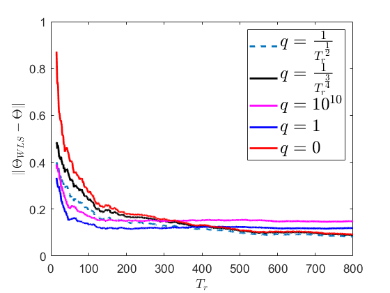
Figure 1: Scenario 1: Both $T_{r}$ and $T_{p}$ increase over time ($T_{p}=3T_{r}$). Choosing $q=\mathcal{O}(\frac{1}{\sqrt{T_{r}}})$ strikes a good balance between reducing error when $T_{r}$ is small and ensuring consistency when $T_{r}$ is large

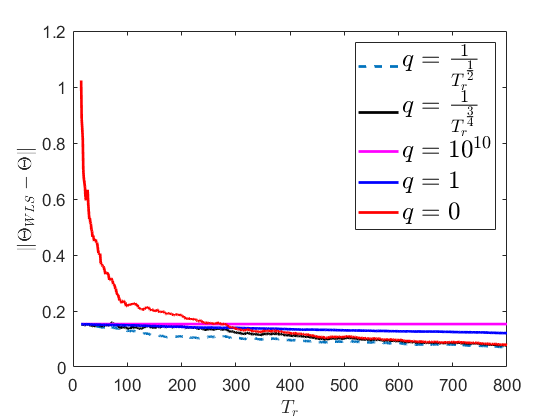
Figure 2: Scenario 2: $T_{p}$ is fixed, and $T_{r}$ increases over time. Having $q$ diminish with $T_{r}$ could reduce the error when $T_{r}$ is small, and avoid unwanted bias from the auxiliary system when $T_{r}$ is large

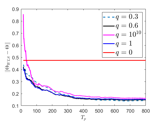
Figure 3: Scenario 3: $T_{r}$ is fixed, and $T_{p}$ increases over time. Setting $q$ to be relatively balanced could make the error smaller than the extreme cases ($q=0,10^{10}$)

V-A1 Scenario 1: Both $T_{r}$ and $T_{p}$ are increasing

In the first experiment, we set the length of the trajectory from the auxiliary system be $T_{p}=3T_{r}$. In practice, one may encounter such a scenario when gathering data from the true system is time consuming or costly, whereas gathering data from an auxiliary system (such as a simulator) is faster or cheaper.

In Fig. 3, we plot the estimation error $\|\Theta-\Theta_{WLS}\|$ versus $T_{r}$ using different weight parameters $q$. As expected, when one does not have enough data from the true system ($T_{r}$ is small), setting $q>0$ leads to a smaller estimation error of system matrices. However, the curve for $q=1$ and $q=10^{10}$ (corresponding to treating all samples equally and paying almost no attention to the samples from the true system, respectively) eventually plateau and incur more error than not using the the auxiliary data ($q=0$). This phenomenon matches with the theoretical guarantee in Theorem 1. Specifically, when $q$ is a nonzero constant and both $T_{p}$ and $T_{r}$ are increasing in a linear relationship, it can be verified that the upper bound in Theorem 1 will not go to zero as $T_{r}$ increases. In other words, there is no need to attach high importance to the auxiliary data when one has enough data from the true system. In contrast, setting $q$ to be diminishing with $T_{r}$ could perform consistently better than $q=0$ in this example, even when $T_{r}$ becomes large. Indeed, one can choose $q=\mathcal{O}(\frac{1}{\sqrt{T_{r}}})$ in the upper bound given by (15) in Theorem 1, and show that the upper bound becomes $\mathcal{O}(\frac{1}{\sqrt{T_{r}}})$. Thus, the estimation error tends to zero as $T_{r}$ increases to infinity.

Key Takeaway: When $T_{p}$ and $T_{r}$ are both increasing linearly, having $q$ diminish with $T_{r}$ with a rate of $\mathcal{O}(\frac{1}{\sqrt{T_{r}}})$ helps to reduce the system identification error when $T_{r}$ is small (by leveraging data from the auxiliary system), and avoids excessive bias from the auxiliary system when $T_{r}$ is large.

V-A2 Scenario 2: $T_{p}$ is fixed but $T_{r}$ is increasing

For the second experiment, we fix the number of samples from the auxiliary system to be $T_{p}=2400$, and look at what happens as the number of samples from the true system increases. In practice, one may encounter such a scenario when the system dynamics change at some point in time (e.g., due to faults). In this case, the true system we want to learn is the one after the fault, and the auxiliary system is the one prior to the fault. Consequently, the data from the old (auxiliary) system may not accurately represent the new (true) system dynamics. While one can collect data from the new system dynamics, leveraging the old data might be beneficial in this case.

In Fig. 3, we plot the estimation error versus $T_{r}$ for different weight parameters $q$. As expected, setting $q>0$ leads to a much smaller error during the initial phase when $T_{r}$ is small. This can be confirmed by Theorem 1 since the overall estimation error is essentially the error due to the model difference. Namely, the auxiliary data helps to build a good initial estimate when $T_{r}$ is small. When we set the weight to be $q=10^{10}$, we are paying little attention to the samples from the true system, i.e., we are not gaining any new information as we collect more data from the true system. Consequently, the error is almost a flat line as $T_{r}$ increases when $q=10^{10}$. As can be observed from Theorem 1, when $T_{p}$ is fixed, we can always make the error go to $0$ as we increase $T_{r}$, using the weights we selected in this experiment. However, when $q$ is set to be too large, it could make the error even larger due to the model difference (or bias) introduced by the auxiliary system. This is captured by Theorem 1 since when $q$ is set to be too large (such that $qT_{p}$ is large compared to $T_{r}$), even when $T_{r}$ becomes larger, the second term in the error bound (15) (capturing model difference) is still large.

Key Takeaway: When $T_{p}$ is fixed and large, and $T_{r}$ increases over time, setting $q$ to be nonzero builds a good initial estimate for the true system dynamics when we have little data from the true system. Again, having $q$ diminish with $T_{r}$ could reduce the system identification error when $T_{r}$ is small, and avoid unwanted bias from the auxiliary system when $T_{r}$ is large.

V-A3 Scenario 3: $T_{r}$ is fixed but $T_{p}$ is increasing

In the last experiment, we fix the number of samples from the true system to be $T_{r}=50$. As discussed earlier, one may encounter such a scenario when one has only a limited amount of time to gather data from the true system. Consequently, leveraging information from other “similar” systems (e.g., from a reasonably accurate simulator) could be helpful to augment the data. This is the most subtle case, since Theorem 1 does not ensure consistency when $T_{r}$ is fixed.

In Fig. 3, we plot the the estimation error versus $T_{p}$ using different weight parameters $q$. As it can be seen, setting $q=0$ (not using the auxiliary samples) gives a flat line, which represents the error we can achieve purely based on $T_{r}=50$ samples from the true system. When $q=10^{10}$, we are paying little attention to the true system, and essentially learning the dynamics of the auxiliary system. In contrast, the results for $q=1,0.6,0.3$ suggest that setting a relatively balanced weight $q$ to the auxiliary data could make the error smaller than the two extreme cases ($q=0,10^{10}$) in this example. However, in practice, one may want to leverage a cross-validation process to tune the hyper-parameter $q$, when there is not enough prior knowledge about the dynamics of the true system and the auxiliary system.

Key Takeaway: Although consistency cannot be guaranteed when $T_{r}$ is fixed and $T_{p}$ increases over time, a relatively balanced $q$ could make the error smaller than the extreme cases ($q=0,10^{10}$).

V-B Selecting $q$ based on Theorem 2

In this section, we study selecting the weight parameter $q$ using Theorem 2 using a fixed regularization parameter $\lambda$. We plot the true error $\|\Theta-\Theta_{WLS}\|$ and the theoretical data-dependent bound in Theorem 2 as a function of weight parameter $q$ varying from $0$ to $2$, where the increment is set to be $0.01$. This corresponds to the situation where some upper bounds on $\|\delta_{\Theta}\|,\bar{\sigma}_{w}$ and $\hat{\sigma}_{w}$ are available (as discussed in Remark 5). We set the confidence parameter to be $\delta=0.01$, and all other parameters in Theorem 2 are assumed to be known exactly for simplicity. The system matrices of the true system and the auxiliary system are set to be

$$\bar{A}=\begin{bmatrix}0.6&0.5&0.4\\ 0&0.5&0.4\\ 0&0&0.4\\ \end{bmatrix},\indent\bar{B}=\begin{bmatrix}1&0.5\\ 0.5&1\\ 0.5&0.5\\ \end{bmatrix},$$ (31)

$$\hat{A}=\begin{bmatrix}0.7&0.5&0.4\\ 0&0.5&0.4\\ 0&0&0.4\\ \end{bmatrix},\indent\hat{B}=\begin{bmatrix}1+\mathbf{\Delta}&0.5\\ 0.5&1\\ 0.5&0.5\\ \end{bmatrix}.$$ (32)

We set the regularization parameter to be $\lambda=1$. We set $\bar{x}_{0},\hat{x}_{0},\bar{u}_{t},\hat{u}_{t},\bar{w}_{t},\hat{w}_{t}$ to be zero mean Gaussian random vectors, where $\sigma_{\bar{x}},\sigma_{\hat{x}},\sigma_{\bar{u}},\sigma_{\hat{u}}$ are set to be $1$. The trajectory lengths are set to be $T_{r}=10,T_{p}=50$, and the number of trajectories from the auxiliary system is set to be $N_{p}=20$. The values of $\mathbf{\Delta},\sigma_{\bar{w}},\sigma_{\hat{w}},N_{r}$ are specified under the figures.

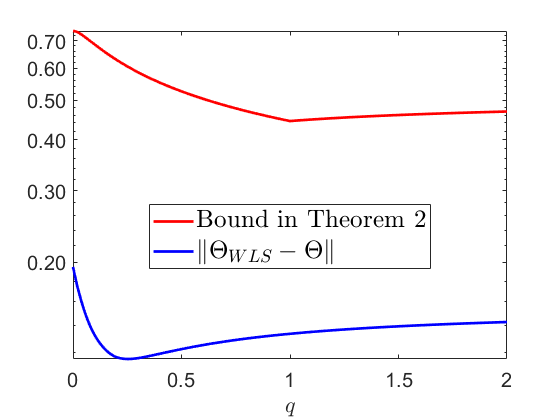
Figure 4: Baseline case 1: $\mathbf{\Delta}=0.1,\sigma_{\bar{w}}=\sigma_{\hat{w}}=1,N_{r}=20$. An intermediate value of $q$ is optimal

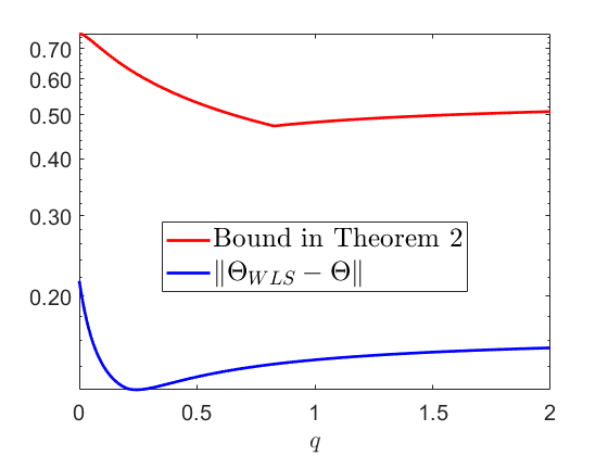
Figure 5: Baseline case 2: $\mathbf{\Delta}=0.11,\sigma_{\bar{w}}=1,\sigma_{\hat{w}}=1.1,N_{r}=19$. An intermediate value of $q$ is optimal

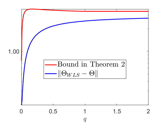
Figure 6: Large model difference: $\mathbf{\Delta}=3,\sigma_{\bar{w}}=\sigma_{\hat{w}}=1,N_{r}=20$. In this case, it is optimal to not use data from the auxiliary system ($q=0$)

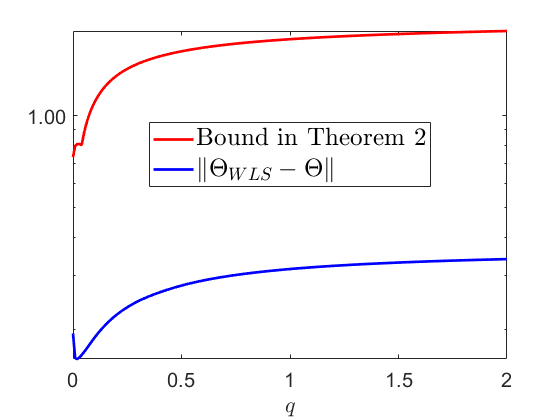
Figure 7: Noisy auxiliary system: $\mathbf{\Delta}=0.1,\sigma_{\bar{w}}=1,\sigma_{\hat{w}}=5,N_{r}=20$. In this case, it is optimal to not use data from the auxiliary system ($q=0$)

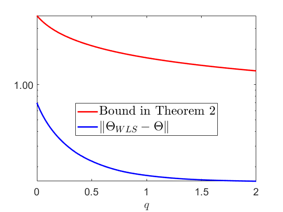
Figure 8: Noisy true system: $\mathbf{\Delta}=0.1,\sigma_{\bar{w}}=5,\sigma_{\hat{w}}=1,N_{r}=20$. In this case, it is optimal to assign higher weight to the auxiliary system ($q=2$)

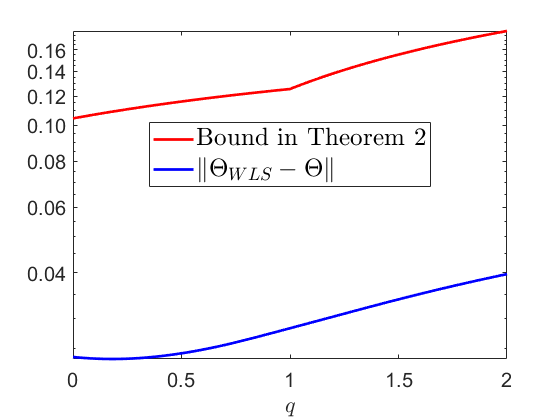
Figure 9: Large number of true samples: $\mathbf{\Delta}=0.1,\sigma_{\bar{w}}=\sigma_{\hat{w}}=1,N_{r}=1200$. In this case, it is optimal to not use data from the auxiliary system ($q=0$)

As can be seen in Fig. 9 and Fig. 9, setting $q$ to be non-zero could result in smaller error bounds, which show the benefits of leveraging the auxiliary data. However, for the values of the weight $q$ we plotted, the optimal weights that obtain the smallest error bounds in Theorem 2 do not align with the optimal weights $q$ that minimize the true error $\|\Theta-\Theta_{WLS}\|$. Such mismatches could be due to the conservativeness of the bound. On the other hand, the optimal weight from the bound still captures how the true optimal weight should scale. As can be seen in Fig. 9, Fig. 9, and Fig. 9, the optimal weight for both the bound and the true error tend to be small when (1) the model difference is large; or (2) the auxiliary system becomes much more noisy; or (3) when one has a large number of samples from the true system. Such empirical results also match with our observations in Corollary 1 when $\lambda=0$. In Fig. 9, both the optimal weight from our bound and the true optimal weight are greater than $1$, since the true system is very noisy and hence the data from the true system tend to be less informative compared to the data from the auxiliary system. We further note that, in practice, selecting the exact optimal weight $q$ that minimizes $\|\Theta_{WLS}-\Theta\|$ is very hard, and one would instead focus on selecting a relatively good weight $q$. The weight that results in a small error bound can be integrated with techniques like robust control to improve the overall system performance guarantee.

VI Conclusion

In this paper, we provided finite sample analysis of system identification using a weighted least squares approach, when one has an auxiliary system that shares similar dynamics as the true system we want to learn. The analysis improves the result in [21] as we show the error due to noise can be reduced by increasing either the number of trajectories or the trajectory length of the true system and the auxiliary system, or both. Our analysis provides insights on the benefits of using the auxiliary system, and how to weight the data from the auxiliary system. We also provided a data-dependent bound that is computable when some prior knowledge about the systems is available, which is tighter and can be used to determine the appropriate weight parameter in the training process.

There are several directions for future research. First, it would be interesting to study how to leverage data from multiple auxiliary systems, which corresponds to the scenario where collecting abundant samples from the same auxiliary system is impossible. Second, as shown in [13], the least squares estimator is consistent for certain types of unstable systems even if multiple trajectories of data are not available. It would be interesting to study how to capture that in our analysis. Finally, it would be interesting to study how to leverage the idea of learning from similar systems/transfer learning in control-related problems [34].

Appendix

Definition 2.

Let $(T,d)$ be a metric space. Consider a subset $K\subset T$ and let $\epsilon>0$. A subset $\mathbf{N}\subseteq K$ is called an $\epsilon$-net of $K$ if every point in $K$ is within distance $\epsilon$ of some point of $\mathbf{N}$, i.e.,

$$\forall x\in K\quad\exists x_{0}\in\mathbf{N}:d(x.x_{0})\leq\epsilon.$$

Lemma 6.

([35, Corollary 4.2.13]) Let $\epsilon>0$, and let $\mathbf{N}(\mathcal{S}^{n-1},\epsilon)$ be the smallest possible cardinality of an $\epsilon$-net of the unit Euclidean sphere $\mathcal{S}^{n-1}$. We have the following inequality:

$$\mathbf{N}(\mathcal{S}^{n-1},\epsilon)\leq(\frac{2}{\epsilon}+1)^{n}.$$

Lemma 7.

([35, Lemma 4.4.1]) Let $A$ be an $m$ by $n$ matrix and $\epsilon\in[0,1)$. Then, for any $\epsilon$-net $\mathbf{N}$ of the sphere $\mathcal{S}^{n-1}$, we have

$$\|A\|\leq\frac{1}{1-\epsilon}\cdot\sup_{x\in\mathbf{N}}\|Ax\|.$$

Lemma 8.

([36, Lemma 3]) Let $A\in\mathbb{R}^{n\times n}$ and $B\in\mathbb{R}^{n\times n}$ be positive semidefinite matrices. If $A\preceq B$, then we have $A^{-1}\succeq B^{-1}$.

Lemma 9.

([36, Theorem 2]) Let $A\in\mathbb{R}^{n\times n}$ and $B\in\mathbb{R}^{n\times n}$ be positive semidefinite matrices. If $A\preceq B$, then we have $A^{\frac{1}{2}}\preceq B^{\frac{1}{2}}$.

Lemma 10.

Let $A\in\mathbb{R}^{n\times n}$ and $B\in\mathbb{R}^{n\times n}$ be positive semidefinite matrices. Let $C\in\mathbb{R}^{n\times m}$. If $A\preceq B$, then we have

$$\|A^{\frac{1}{2}}C\|\leq\|B^{\frac{1}{2}}C\|.$$

Proof.

From $A\preceq B$, we have

$$C^{\prime}AC\preceq C^{\prime}BC,$$

which implies

$$\|A^{\frac{1}{2}}C\|=\sqrt{\lambda_{max}(C^{\prime}AC)}\leq\sqrt{\lambda_{max}(C^{\prime}BC)}=\|B^{\frac{1}{2}}C\|.$$

∎

Proposition 2.

Assume that $\rho(\bar{A})<1$ and $\rho(\hat{A})<1$. For all $t\geq 0$, we have the following inequalities:

$$\operatorname{tr}(\bar{G}_{t}) \leq\frac{n\bar{\kappa}^{2}}{1-\bar{\gamma}^{2}}+\frac{n\bar{\kappa}^{2}\|\bar{B}\|^{2}}{1-\bar{\gamma}^{2}},$$

$$\operatorname{tr}(\hat{G}_{t}) \leq\frac{n\hat{\kappa}^{2}}{1-\hat{\gamma}^{2}}+\frac{n\hat{\kappa}^{2}\|\hat{B}\|^{2}}{1-\hat{\gamma}^{2}},$$

where $\bar{G}_{t}$ and $\hat{G}_{t}$ are defined in (8), and $\bar{\kappa}\geq 1,\hat{\kappa}\geq 1,\rho(\bar{A})<\bar{\gamma}<1,\rho(\hat{A})<\hat{\gamma}<1$ are finite constants that satisfy $\|\bar{A}^{i}\|\leq\bar{\kappa}\bar{\gamma}^{i}$ and $\|\hat{A}^{i}\|\leq\hat{\kappa}\hat{\gamma}^{i}$ for all $i\geq 0$.

Proof.

We only consider the term $\operatorname{tr}(\bar{G}_{t})$ as the term $\operatorname{tr}(\hat{G}_{t})$ is essentially the same. We have

$$\operatorname{tr}(\bar{G}_{t}) \leq n\|\bar{G}_{t}\|=n\|\sum_{i=0}^{t}\bar{A}^{i}\bar{A}^{i}{{}^{\prime}}+\sum_{i=0}^{t-1}\bar{A}^{i}\bar{B}\bar{B}^{\prime}\bar{A}^{i}{{}^{\prime}}\|$$

$$\leq n\sum_{i=0}^{t}\|\bar{A}^{i}\|^{2}+n\|\bar{B}\|^{2}\sum_{i=0}^{t-1}\|\bar{A}^{i}\|^{2}.$$

From the Gelfand formula [37], there always exist finite constants $\bar{\kappa}\geq 1$ and $\rho(\bar{A})<\bar{\gamma}<1$ such that $\|\bar{A}^{i}\|\leq\bar{\kappa}\bar{\gamma}^{i}$ for all $i\geq 0$. Consequently, we have

$$n\sum_{i=0}^{t}\|\bar{A}^{i}\|^{2}+n\|\bar{B}\|^{2}\sum_{i=0}^{t-1}\|\bar{A}^{i}\|^{2} \leq\frac{n\bar{\kappa}^{2}}{1-\bar{\gamma}^{2}}+\frac{n\bar{\kappa}^{2}\|\bar{B}\|^{2}}{1-\bar{\gamma}^{2}}.$$

∎

Lei Xin received the B.S. degree in electrical and computer engineering in 2018 from Purdue University, West Lafayette, IN, USA, where he graduated with highest distinction. He is currently working toward the Ph.D. degree in electrical and computer engineering at the same institution. He was a finalist for the Best Student Paper Award at the 2022 American Control Conference. His research interests include machine learning, system identification, and optimization.

Lintao Ye is a Lecturer in the School of Artificial Intelligence and Automation at the Huazhong University of Science and Technology, Wuhan, China. He received his M.S. degree in Mechanical Engineering in 2017, and his Ph.D. degree in Electrical and Computer Engineering in 2020, both from Purdue University, IN, USA. He was a Postdoctoral Researcher at the University of Notre Dame, IN, USA. His research interests are in the areas of optimization algorithms, control theory, estimation theory, and network science.

George T.-C. Chiu is a Professor in the School of Mechanical Engineering with courtesy appointments in the School of Electrical and Computer Engineering and the Department of Psychological Sciences at Purdue University. Dr. Chiu received the B.S. degree in Mechanical Engineering from the National Taiwan University in 1985 and the M.S. and Ph.D. degrees in Mechanical Engineering from the University of California at Berkeley, in 1990 and 1994, respectively. Before joining Purdue, he worked for Hewlett-Packard and was part of the team that developed the first inkjet multifunction device. From September 2011 to June 2014, he served as the Program Director for the Control Systems Program at the US National Science Foundation. Dr. Chiu’s current research interests are mechatronics and dynamic systems and control with applications to digital printing and imaging systems, digital fabrications and functional printing, human motor control, motion and vibration perception and control. He has co-authored more than 180 peer-reviewed publications as well as 16 US and international patents. He received the 2012 NSF Director’s Collaboration Award, the 2010 IEEE Transactions on Control System Technology Outstanding Paper Award, Purdue University Teaching for Tomorrow Award, College of Engineering 2010 Faculty Engagement/Service Excellence Award and 2006 Faculty Research Team Excellence Award. He served as the Editor-in-Chief for the IEEE/ASME Transactions on Mechatronics from 2017-19 and the Editor for the Journal of Imaging Science and Technology from 2012-14. He is a Fellow of ASME and a Fellow of the Society for Imaging Science and Technology (IS&T).

Shreyas Sundaram is the Marie Gordon Associate Professor in the Elmore Family School of Electrical and Computer Engineering at Purdue University. He received his MS and PhD degrees in Electrical Engineering from the University of Illinois at Urbana-Champaign in 2005 and 2009, respectively. He was a Postdoctoral Researcher at the University of Pennsylvania from 2009 to 2010, and an Assistant Professor in the Department of Electrical and Computer Engineering at the University of Waterloo from 2010 to 2014. He is a recipient of the NSF CAREER award, and an Air Force Research Lab Summer Faculty Fellowship. At Purdue, he received the Hesselberth Award for Teaching Excellence and the Ruth and Joel Spira Outstanding Teacher Award. At Waterloo, he received the Department of Electrical and Computer Engineering Research Award and the Faculty of Engineering Distinguished Performance Award. He received the M. E. Van Valkenburg Graduate Research Award and the Robert T. Chien Memorial Award from the University of Illinois, and he was a finalist for the Best Student Paper Award at the 2007 and 2008 American Control Conferences. His research interests include network science, analysis of large-scale dynamical systems, fault-tolerant and secure control, linear system and estimation theory, game theory, and the application of algebraic graph theory to system analysis.

References

- [1] L. Ljung, “System identification,” Wiley encyclopedia of electrical and electronics engineering, pp. 1–19, 1999.
- [2] D. Bauer, M. Deistler, and W. Scherrer, “Consistency and asymptotic normality of some subspace algorithms for systems without observed inputs,” Automatica, vol. 35, no. 7, pp. 1243–1254, 1999.
- [3] M. Jansson and B. Wahlberg, “On consistency of subspace methods for system identification,” Automatica, vol. 34, no. 12, pp. 1507–1519, 1998.
- [4] T. Knudsen, “Consistency analysis of subspace identification methods based on a linear regression approach,” Automatica, vol. 37, no. 1, pp. 81–89, 2001.
- [5] S. Dean, H. Mania, N. Matni, B. Recht, and S. Tu, “Regret bounds for robust adaptive control of the linear quadratic regulator,” Advances in Neural Information Processing Systems, vol. 31, 2018.
- [6] ——, “On the sample complexity of the linear quadratic regulator,” Foundations of Computational Mathematics, pp. 1–47, 2019.
- [7] L. Ye, H. Zhu, and V. Gupta, “On the sample complexity of decentralized linear quadratic regulator with partially nested information structure,” IEEE Transactions on Automatic Control, 2022.
- [8] M. Simchowitz, H. Mania, S. Tu, M. I. Jordan, and B. Recht, “Learning without mixing: Towards a sharp analysis of linear system identification,” in Proc. Conference On Learning Theory, 2018, pp. 439–473.
- [9] S. Oymak and N. Ozay, “Non-asymptotic identification of LTI systems from a single trajectory,” in American control conference. IEEE, 2019, pp. 5655–5661.
- [10] M. Simchowitz, R. Boczar, and B. Recht, “Learning linear dynamical systems with semi-parametric least squares,” in Proc. Conference on Learning Theory, 2019, pp. 2714–2802.
- [11] T. Sarkar, A. Rakhlin, and M. A. Dahleh, “Nonparametric finite time LTI system identification,” arXiv preprint arXiv:1902.01848, 2019.
- [12] M. K. S. Faradonbeh, A. Tewari, and G. Michailidis, “Finite time identification in unstable linear systems,” Automatica, vol. 96, pp. 342–353, 2018.
- [13] T. Sarkar and A. Rakhlin, “Near optimal finite time identification of arbitrary linear dynamical systems,” in Proc. International Conference on Machine Learning, 2019, pp. 5610–5618.
- [14] S. Fattahi and S. Sojoudi, “Data-driven sparse system identification,” in Proc. Allerton Conference on Communication, Control, and Computing, 2018, pp. 462–469.
- [15] Y. Sun, S. Oymak, and M. Fazel, “Finite sample system identification: Optimal rates and the role of regularization,” in Proc. Learning for Dynamics and Control Conference, 2020, pp. 16–25.
- [16] Y. Zheng and N. Li, “Non-asymptotic identification of linear dynamical systems using multiple trajectories,” IEEE Control Systems Letters, vol. 5, no. 5, pp. 1693–1698, 2020.
- [17] L. Xin, G. Chiu, and S. Sundaram, “Learning the dynamics of autonomous linear systems from multiple trajectories,” in 2022 American Control Conference (ACC). IEEE, 2022, pp. 3955–3960.
- [18] S. Tu, R. Frostig, and M. Soltanolkotabi, “Learning from many trajectories,” arXiv preprint arXiv:2203.17193, 2022.
- [19] S. J. Pan and Q. Yang, “A survey on transfer learning,” IEEE Transactions on knowledge and data engineering, vol. 22, no. 10, pp. 1345–1359, 2009.
- [20] H. Bastani, “Predicting with proxies: Transfer learning in high dimension,” Management Science, vol. 67, no. 5, pp. 2964–2984, 2021.
- [21] L. Xin, L. Ye, G. Chiu, and S. Sundaram, “Identifying the dynamics of a system by leveraging data from similar systems,” in 2022 American Control Conference (ACC). IEEE, 2022, pp. 818–824.
- [22] A. E. Hoerl and R. W. Kennard, “Ridge regression: Biased estimation for nonorthogonal problems,” Technometrics, vol. 12, no. 1, pp. 55–67, 1970.
- [23] A. Cassel, A. Cohen, and T. Koren, “Logarithmic regret for learning linear quadratic regulators efficiently,” in International Conference on Machine Learning. PMLR, 2020, pp. 1328–1337.
- [24] M. Rudelson and R. Vershynin, “Hanson-wright inequality and sub-gaussian concentration,” Electronic Communications in Probability, vol. 18, pp. 1–9, 2013.
- [25] F. Zhang and Q. Zhang, “Eigenvalue inequalities for matrix product,” IEEE Transactions on Automatic Control, vol. 51, no. 9, pp. 1506–1509, 2006.
- [26] H. Zhang and S. X. Chen, “Concentration inequalities for statistical inference,” arXiv preprint arXiv:2011.02258, 2020.
- [27] D. Dadush, C. Guzmán, and N. Olver, “Fast, deterministic and sparse dimensionality reduction,” in Proceedings of the Twenty-Ninth Annual ACM-SIAM Symposium on Discrete Algorithms. SIAM, 2018, pp. 1330–1344.
- [28] K. Moshksar, “On the absolute constant in hanson-wright inequality,” arXiv preprint arXiv:2111.00557, 2021.
- [29] Y. Abbasi-Yadkori, D. Pál, and C. Szepesvári, “Improved algorithms for linear stochastic bandits,” Advances in neural information processing systems, vol. 24, 2011.
- [30] N. Matni and S. Tu, “A tutorial on concentration bounds for system identification,” in 2019 IEEE 58th Conference on Decision and Control (CDC). IEEE, 2019, pp. 3741–3749.
- [31] A. Tsiamis and G. J. Pappas, “Finite sample analysis of stochastic system identification,” in Conference on Decision and Control (CDC). IEEE, 2019, pp. 3648–3654, arXiv:1903.09122.
- [32] P. Refaeilzadeh, L. Tang, and H. Liu, “Cross-validation.” Encyclopedia of database systems, vol. 5, pp. 532–538, 2009.
- [33] B. W. Silverman, Density estimation for statistics and data analysis. Routledge, 2018.
- [34] L. Li, C. De Persis, P. Tesi, and N. Monshizadeh, “Data-based transfer stabilization in linear systems,” arXiv preprint arXiv:2211.05536, 2022.
- [35] R. Vershynin, High-dimensional probability: An introduction with applications in data science. Cambridge university press, 2018, vol. 47.
- [36] N. Chan and M. K. Kwong, “Hermitian matrix inequalities and a conjecture,” The American Mathematical Monthly, vol. 92, no. 8, pp. 533–541, 1985.
- [37] R. A. Horn and C. R. Johnson, “Topics in matrix analysis, 1991,” Cambridge University Presss, Cambridge, vol. 37, p. 39, 1991.