Performative Recommendation: Diversifying Content via Strategic Incentives

Abstract

The primary goal in recommendation is to suggest relevant content to users, but optimizing for accuracy often results in recommendations that lack diversity. To remedy this, conventional approaches such as re-ranking improve diversity by presenting more diverse items. Here we argue that to promote inherent and prolonged diversity, the system must encourage its creation. Towards this, we harness the performative nature of recommendation, and show how learning can incentivize strategic content creators to create diverse content. Our approach relies on a novel form of regularization that anticipates strategic changes to content, and penalizes for content homogeneity. We provide analytic and empirical results that demonstrate when and how diversity can be incentivized, and experimentally demonstrate the utility of our approach on synthetic and semi-synthetic data.

1 Introduction

Recommendation has become a key driving force in determining what content we are exposed to, and ultimately, which we consume (MacKenzie et al., 2013; Ursu, 2018). But despite the commercial success of modern recommendation systems, a known shortcoming is that recommendations tend to be insufficiently diverse, with content homogeneity becoming more pronounced over time; this has been a longstanding issue in the field for over two decades (Carbonell & Goldstein, 1998; Bradley & Smyth, 2001). Diversity is important in recommendation not only for improving recommendation quality (Vargas & Castells, 2014; Kaminskas & Bridge, 2016) and user satisfaction (Herlocker et al., 2004; Ziegler et al., 2005; McNee et al., 2006; Hu & Pu, 2011; Wu et al., 2018; Dean et al., 2020), but also because a lack of diversity can lead to inequity across content creators, which often hurts the ‘long-tail’ of non-mainstream suppliers (Yin et al., 2012; Burke, 2017; Singh & Joachims, 2018; Abdollahpouri et al., 2019b; Mladenov et al., 2020; Wang & Joachims, 2021). From the perspective of the recommendation platform, an inability to diversify content translates into an inability to utilize the full potential that lies in the natural variation of user preferences for promoting system goals (Anderson, 2006; Yin et al., 2012). This has lead to widespread interest in developing methods for making recommendations more diverse (Kunaver & Požrl, 2017).

The common approach for diversifying recommendations is to apply some post-processing procedure that re-ranks the output of a conventionally-trained ranking model—which is optimized for predicting user-item relevance—to be more diverse, for example by traversing the ranked list and removing items which are similar to higher-ranked items (Carbonell & Goldstein, 1998; Ziegler et al., 2005; Sha et al., 2016). This simple heuristic approach has been shown to be quite effective—at least when considering a given ranked list, and at one point in time. But recommendation is inherently a dynamic process: here we argue that post-hoc methods may not suffice for promoting diversity in the long run.

To see why, consider that re-ranking (and similar approaches) are designed to diversify the presentation of content—not content itself. Presenting diverse content may help in the specific instance it targets, but does not change the pool of available items, nor does it account for any downstream affects of recommendation. Recent work has shown that one drawback of using prediction as the basis for recommendation is that it causes homogenization (Chaney et al., 2018); here we argue that rearranging predicted items to form the appearance of diversity does not remedy this.

As an alternative, we propose to encourage the creation of diverse content, so that the set of available items becomes inherently more diverse. In this way, we aim to target the cause—rather than the symptom. Our main observation is that content is shaped by content creators, who seek to maximize exposure to their items (Ben-Porat et al., 2020; Hron et al., 2022), and hence likely to modify content in ways which promote their item’s predicted relevance (or ‘score’). Since the goal of learning is to infer such scores, this gives the learning system leverage in shaping the incentives of content creators. Here we propose to utilize this power to incentivize for the creation of more diverse content.

Towards this, we draw connections to the related literature on strategic learning (Brückner et al., 2012; Hardt et al., 2016), and model content creators as gaining utility from the score given to their items by the learned predictive model. Content creators can then improve their utility by strategically modifying their items to obtain a higher score. Thus, a learned predictive model determines not only what items are recommended to which users—but also creates incentives for content creators, which can promote change (Ben-Porat & Tennenholtz, 2018; Jagadeesan et al., 2022). This provides the system with the potential power to steer the collection of renewing items—over time, and with proper incentivization—towards diversity (Hardt et al., 2022).

To study when and how the system can effectively exercise its power, we cast recommendation as an instance of performative prediction (Perdomo et al., 2020), which subsumes and extends strategic learning to a temporal setting where repeated learning causes the underlying data to shift over time. Focusing on retraining dynamics, we study when and how learning can be used to incentivize the creation and preservation of diversity. In retraining, our only means for driving incentivizes derives from how we retrain, i.e., from our criterion for choosing the predictive model at each round. Since retraining aims for models that are predictively accurate, our goal will be to provide recommendations that are accurate and diverse. But diversity and accuracy can be at odds; hence, we seek to understand how they relate, and to propose ways in which their tradeoff can be optimally exploited.

We begin with a basic analysis demonstrating the mechanisms through which incentives and diversity relate within our setup. We then propose a learning objective that allows to balance ranking accuracy (and in particular NDCG) with diversity through a novel form of regularization, which we use to maximize diversity under accuracy constraints. Our proposed diversity regularizer has two main benefits. First, it is differentiable, and hence can be optimized using gradient methods. Second, it can be applied to strategically-modified inputs; this equips our objective with the ability to anticipate the strategic responses of content creators, and hence, to encourage predictive rules that incentivize diversity. Our proposed strategic response operator is also differentiable; thus, and using recent advances in differentiable learning-to-rank, our entire strategic learning objective becomes differentiable, and can be efficiently optimized end-to-end.

Using our proposed learning framework, we empirically demonstrate how properly accounting for strategic incentives can improve diversity—and how neglecting to do so can lead to homogenization. We begin with a series of synthetic experiments, each designed to study a different aspect of our setup, such as the role of time, the natural variation in user preferences, and the cost of applying strategic updates. We then evaluate our approach in a semi-synthetic environment using real data (Yelp restaurants) and simulated responses. Our results demonstrate the ability of strategically-aware retraining to bolster diversity, and illustrate the importance of incentivizing the creation of diversity. All code is made publicly available at: https://github.com/itayeilat/Performative-Recommendation.

1.1 Related work

Diversity in recommendation.   The literature on diversity in recommendation is extensive; here we present a relevant subset. Early approaches propose to diversify via re-ranking (Carbonell & Goldstein, 1998; Bradley & Smyth, 2001; Ziegler et al., 2005), an approach that remains to be in widespread use today (Abdollahpouri et al., 2019a). More recent methods include diversifying via functional optimization (Zhang & Hurley, 2008) or integration within matrix factorization (Su et al., 2013; Hurley, 2013; Cheng et al., 2017). Diversity has also been studied in sequential (Kim et al., 2019), conversational (Fu et al., 2021), and adversarial bandit (Brown & Agarwal, ) settings. The idea of using regularization to promote secondary objectives in recommendation has been applied for controlling popularity bias (Abdollahpouri et al., 2017), enhancing neutrality (Kamishima et al., 2014), and promoting equal opportunity (Zhu et al., 2021). For diversity, Wasilewski & Hurley (2016) apply regularization, but assume that the system has direct control over (latent) item features; this is crucially distinct from our setting in which the system can only indirectly encourage content creators to apply changes.

Strategic learning.   There has been much recent interest in studying learning in the presence of strategic behavior. Hardt et al. (2016) propose strategic classification as a framework for studying classification tasks in which users (who are the targets of prediction) can modify their features—at a cost—to obtain favorable predictions. This is based on earlier formulations by Brückner & Scheffer (2009); Brückner et al. (2012), with recent works extending the framework to settings in which users act on noisy (Jagadeesan et al., 2021) or missing information (Ghalme et al., 2021; Bechavod et al., 2022), have broader interests (Levanon & Rosenfeld, 2022), or are connected by a graph (Eilat et al., 2022). Since we model content creators as responding to a scoring rule, our work pertains to the subliterature on strategic regression, in which user utility derives from a continuous function (Rosenfeld et al., 2020; Tang et al., 2021; Harris et al., 2021; Bechavod et al., 2022), and strategic behavior is often assumed to also affect outcomes (Shavit et al., 2020; Harris et al., 2022). Within this field, our framework is unique in that it considers content creators—rather than end-users—as the focal strategic entities. The main distinction is that this requires learning to account for the joint behavior of all strategic agents (rather than each individually), which even for linear score functions results in complex behavioral patters (c.f. standard settings in which linearity implies uniform movement (Liu et al., 2022)). Regularization has been used to control incentives in Rosenfeld et al. (2020); Levanon & Rosenfeld (2021), but in distinct settings and towards different goals (i.e., unrelated to recommendation or diversity), and for user responses that fully decompose.

Performativity and incentives.   The current literature on performative learning focuses primarily on macro-level analysis, such as providing sufficient global conditions for retraining to converge (Perdomo et al., 2020; Miller et al., 2021; Brown et al., 2022) or proposing general optimization algorithms (Mendler-Dünner et al., 2020; Izzo et al., 2021; Drusvyatskiy & Xiao, 2022; Maheshwari et al., 2022). In contrast, performativity in our setting emerges from micro-level modeling of strategic agents in a dynamic recommendation environment, and our goal is to address the specific challenges inherent in our focal learning task. Within recommendation, content creators (or ‘supplier’) incentives have also been studied from a game-theoretic perspective (Ben-Porat & Tennenholtz, 2018; Ben-Porat et al., 2019, 2020; Jagadeesan et al., 2022; Hron et al., 2022). Here, focus tends to be on notions of equilibrium, and the system is typically assumed to have direct control over outcomes (e.g., determining allocations or monetary rewards). Our work focuses primarily on learning, and studies indirect incentivization through a learned predictive rule.

2 Problem Setup

Our setup considers a recommendation platform consisting of $m$ users and $n$ items. Items are described by feature vectors $x_{j}\in{\mathbb{R}}^{d}$, $j\in[n]$, and each item $x_{j}$ is owned by a (strategic) content creator $j$. The goal of the system is to learn latent vector representations $u_{i}\in{\mathbb{R}}^{d}$ for each user $i\in[m]$ that are useful for recommending relevant items. As in Hron et al. (2022), we assume all features are constrained to have unit $\ell_{2}$ norm, $\|u\|=\|x\|=1$ (i.e., lie on the unit sphere). This ensures equal treatment across items (by the system) and users (by content creators), and prevents features from growing indefinitely due to strategic updates.

The system makes recommendations by ranking items for each user $i$ using a personalized score function $f_{i}(x)$ as:

$${\bm{r}}_{i}=\operatorname{rank}(f_{i}(x_{1}),\dots,f_{i}(x_{n}))\,\,\quad\forall i\in[m]$$ (1)

where $f_{i}(x)=f(x;u_{i})$ rely on learned user representation vectors $u_{i}$. For a list of items $X$ we denote in shorthand ${\bm{r}}_{i}=\operatorname{rank}(f(X;u_{i}))$. As in most works on strategic learning (e.g., Hron et al., 2022; Jagadeesan et al., 2022; Carroll et al., 2022), we consider linear score functions $f(x;u_{i})=u_{i}^{\top}x$. Overall, the goal of the system is to learn good $f_{1},\dots,f_{n}$ from data, where $u_{1},\dots,u_{n}$ are the learned parameters.

Learning objective.   We measure ranking quality using the standard measure of NDCG evaluated on the top $k$ items, defined as follows. Consider a list of items with relevance scores ${\bm{y}}=(y_{1},\dots,y_{n})$. Let ${\bm{r}}=(r_{1},\dots,r_{n})$ be a ranking, and denote by ${\bm{r}}(\ell)$ the index of the $\ell^{\text{th}}$-ranked item in ${\bm{r}}$. Then the top-$k$ discounted cumulative gain (DCG) is:

$$\mathrm{DCG}_{@k}({\bm{y}},{\bm{r}})=\sum\nolimits_{\ell=1}^{k}\frac{2^{y_{{\bm{r}}(\ell)}}-1}{\log(1+\ell)}$$ (2)

where $2^{y_{j}}-1$ measures the ‘gain’ in relevance from having item $j=r(\ell)$ in the top $k$, and $\log(1+\ell)$ ‘discounts’ its rank. NDCG is then obtained by normalizing relative to the optimal ranking ${\bm{r}}^{*}=\operatorname*{argmax}_{{\bm{r}}}\mathrm{DCG}_{@k}({\bm{y}},{\bm{r}})$. The primary goal of the system is therefore to learn user representations $\{u_{i}\}_{i=1}^{n}$ that optimize average top-$k$ NDCG:

$$\max_{u_{1},\dots,u_{m}}\frac{1}{m}\sum\nolimits_{i=1}^{m}\mathrm{NDCG}_{@{k}}({\bm{y}}_{i},{\bm{r}}_{i})$$ (3)

where ${\bm{r}}_{i}$ is the ranking of items for user $i$ according to $f(x;u_{i})$. For learning, we will assume that the system has access to relevance labels $y_{ij}$ for some user-item pairs $(i,j)$, and the goal is to generalize well to other pairs.

Item diversity.   In addition to ranking accuracy, we will also be interested in measuring and promoting diversity across recommended items. Here we consider intra-list diversity (Ziegler et al., 2005; Vargas & Castells, 2011; Antikacioglu et al., 2019) and focus primarily on cosine similarity as a metric, $\cos(x,x^{\prime})=\frac{x^{\top}x^{\prime}}{\|x\|\|x^{\prime}\|}$, which is appropriate for comparing unit-norm features (Ekstrand et al., 2014; Hron et al., 2022). See Appendix E.4 for an extension of our approach to entropy-based similarity.

For a list of items $X=(x_{1},\dots,x_{K})$ and corresponding ranking ${\bm{r}}$, diversity for the top-$k$ items is defined as:

$${\mathrm{div}_{@{k}}}(X,{\bm{r}})=\frac{1}{k(k-1)}\sum\nolimits_{j,\ell=1}^{k}1-\cos(x_{{\bm{r}}(j)},x_{{\bm{r}}(\ell)})$$ (4)

which takes values in $[0,1]$ (Smyth & McClave, 2001).

Recommendation graph.   In our setting, each user $i$ is associated with a list of $K_{i}$ potentially-relevant items, denoted $X_{i}\subseteq[n]$, and the system’s goal is to choose a subset of $k\leq K_{i}$ items to recommend as a ranked list. Since the same items can appear in multiple lists, it will be useful to consider users and items through a bipartite graph $G=(U,X,E)$, where $(i,j)\in E$ if item $j$ is in user $i$’s list of candidate items. We will also denote $U_{j}=\{i\in[m]\mid(i,j)\in E\}$ and $m_{j}=|U_{j}|$. As we will see, the graph plays a key role in determining the system’s potential for encouraging diversity.

Figure 1: (A) Tradeoff between accuracy and diversity: Consider three items with high ($\huge{\bullet}$), medium ($\huge{\bullet}$), and low ($\huge{\bullet}$) relevance. Learned user embedding $u_{i}$ obtains high $\mathrm{NDCG}_{@{2}}$ (projected points) but low ${\mathrm{div}_{@{2}}}$ (blue sector) (A1). Conversely, $u^{\prime}_{i}$ (note flipped orientation) obtains high diversity, but at the cost of reduced accuracy (A2). (B) Creating diversity with strategic incentives: Consider two items and three users connected by the graph $G$. Initially, both items are similar (light circles), and diversity is low. However, $u_{1}$ and $u_{2}$ incentivize $x_{1}$ and $x_{2}$, respectfully, to move away from each other, results in a more diverse set for $u_{0}$; in this case, without compromising accuracy.

2.1 Strategic content creators

Our key modeling assumption is that items are owned by strategic content creators (or ‘suppliers’) whose aim is to maximize exposure to their items (Hron et al., 2022). Content owners act to increase their item’s score $s(x_{j})$, which is an average over the scores of potentially relevant users:

$$s(x_{j})=\operatorname{avg}\{f(x_{j};u_{i})\mid i\in U_{j}\}$$ (5)

To preserve equity across content creators, we use spherical averaging over user representations $u_{i}$ to maintain unit norm, which pertains to the following form:

$$s(x_{j})={\tilde{v}}_{j}^{\top}x_{j},\,\,\text{ where }\,{\tilde{v}}_{j}=\frac{v_{j}}{\|v_{j}\|},\,v_{j}=\frac{1}{m_{j}}\sum\nolimits_{i\in U_{j}}u_{i}$$

This can be taken to mean that the system reveals normalized scores, so that utility for item $j$ derives from ${\tilde{v}}_{j}$ which describes an ‘average’ user representing all $i\in U_{j}$.

Following the general formalism of strategic classification (Hardt et al., 2016), we assume content creators can modify their item’s features, at a cost, and in response to the learned predictive model. Given a known cost function $c(x,x^{\prime})$, content creators modify items via the best response mapping:

$$x^{f}_{j}=\Delta_{f}(x_{j})\triangleq\operatorname*{argmax}_{x^{\prime}:\|x^{\prime}\|=1}\,s(x^{\prime})-\alpha c(x_{j},x^{\prime})$$ (6)

where the norm constraint ensures that modified items remain on the unit sphere, and throughout we consider quadratic costs, $c(x,x^{\prime})=\|x-x^{\prime}\|_{2}^{2}$. The scaling parameter $\alpha\geq 0$ will allow us to vary the intensity of strategic updates: when $\alpha$ is small, modifications are less restrictive and so $x^{f}_{j}$ can move further away from $x_{j}$, and vice versa.

We consider item modification to be ‘real’, in the sense that changing $x$ can cause $y$ to also change. Following Shavit & Moses (2019); Rosenfeld et al. (2020), we assume labels are determined by an unknown stochastic ground-truth function $f^{*}$ which determines personalized relevance for any counterfactual item $x$ as $y=f^{*}(x;u^{*}_{i})$, where $\{u^{*}_{i}\}_{i=1}^{m}$ are ground-truth user preferences (which are unknown to the learner).

Strategic behavior and diversity.   Eq. (6) reveals how the system can drive incentives: since each content creator $j$ acts to make their item more aligned with ${\tilde{v}}_{j}$, the system can set the $u_{i}$ (which together compose all ${\tilde{v}}_{j}$) to induce ${\tilde{v}}_{j}$-s that vary in their orientation; this incentivizes different content creators to move towards different directions—thus creating diversity, whose potential growth rate is mediated by $\alpha$. Note that even linear $f$ can incentive different items to move in different directions, since (i) due to norm constraints, items will not necessarily move in the direction of the gradient of $f$; and more importantly, (ii) since different items appeal to different users, each ${\tilde{v}}_{j}$ defines a utility function $s(x_{j})=f(x_{j};{\tilde{v}}_{j})$ that is distinct for item $j$. Nonetheless, the ${\tilde{v}}_{j}$ are not disjoint; the connectivity structure in $G$ forms dependencies across the $u_{i}$, which introduce correlations in how items can jointly move (see Fig. 1 (B)).

2.2 Interaction dynamics

We will be interested in studying how learning affects ranking accuracy and diversity over time. As noted, we focus on retraining dynamics, where at each round $t$ the system re-trains its predictive model $\smash{f^{t}}$ on current data $\smash{(x^{t},y^{t})}$, which in our case, is based on strategic responses to the previous model, $\smash{x^{t}_{j}=\Delta_{f^{t-1}}(x^{t-1}_{j})}$. We think of item modification as a process which takes time: In the initial portion of round $t$, users remain to observe $\smash{x_{j}^{t}}$, on which $f^{t}$ was trained; but exposure to $f^{t}$ incentivizes change, and so after some time has passed, content creators publish the modified $\smash{x_{j}^{t+1}}$, for which users provide fresh labels $\smash{y_{ij}^{t+1}}$. Once data has been collected for all modified inputs, the system retrains.

3 Learning and Optimization

The conventional approach for learning to recommend relies on training predictive models to correctly rank items by their relevance. Then, to promote diversity, a post-hoc procedure is typically used to re-rank ${\bm{r}}$, which in our setting can affect diversity by determining which items appear in the top $k$.

The main drawback of re-ranking is that its heuristic nature means that diversifying the list might reduce its relevance, and can cause NDCG to deteriorate substantially. As an alternative, here we pursue a more disciplined approach, in which we directly optimize the joint objective:

$$\max_{u_{1},\dots,u_{m}}\frac{1}{m}\sum_{i=1}^{m}\mathrm{NDCG}_{@{k}}({\bm{y}}_{i},{\bm{r}}_{i})+\lambda\,{\mathrm{div}_{@{k}}}(X_{i},{\bm{r}}_{i})$$ (7)

where ${\bm{r}}_{i}=\operatorname{rank}(f(X_{i};u_{i}))$ is the ranking of items in $X_{i}$ for user $i$, and $\lambda$ trades off between accuracy and diversity. With $\operatorname{div}$ as regularization, we can tune $\lambda$ to obtain a desired balance, or maximize diversity under accuracy constraints. In our experiments we tune $\lambda$ to achieve a predetermined level of NDCG (e.g., 0.9); in this case, regularization serves as a criterion for choosing the most diverse model out of all sufficiently-accurate models.We next describe our approach for optimizing Eq. (7), which sets the ground for our strategically-aware objective.

3.1 Optimization

We propose to optimize Eq. (7) by constructing a differentiable proxy objective, to which we can then apply gradient methods. The key challenge is that Eq. (7) relies on a ranking operator (i.e., for computing NDCG and top-$k$), which is non-differentiable. Our approach adopts and extends Pobrotyn & Bialobrzeski (2021), and makes use of the differentiable sorting operator introduced in Grover et al. (2019). First, consider NDCG. For the numerator, note that the ranking operator ${\bm{r}}(\cdot)$ can be implemented using a corresponding permutation matrix $P$, i.e., $y_{{\bm{r}}(\ell)}=(Py)_{\ell}$. To differentiate through ${\bm{r}}$, we replace $P$ with a ‘smooth’ row-wise softmax permutation matrix, ${\hat{P}}$. We denote by ${\hat{{\bm{r}}}}$ the corresponding soft ranking, computed as ${\hat{{\bm{r}}}}=({\hat{P}}\odot Q)^{\top}\bm{1}$, where $Q_{ij}=i\,\,\forall j$, $\odot$ is the Hadamard product, and $\bm{1}$ is a vector of 1-s. The denominator for $\mathrm{NDCG}_{@{k}}$ requires accessing indexes in $y$ using explicit entries in ${\bm{r}}$; applying ${\hat{{\bm{r}}}}$ instead gives a weighted combination of $y$-s, with most mass concentrated at the correct ${\bm{r}}(\ell)$ when ${\hat{{\bm{r}}}}$ is a good approximation. The summation term is implemented using a soft top-$k$ operator, which we obtain by applying an element-wise scalar sigmoid to ${\bm{r}}$ as:

$$\mathds{1}{\{{r\leq k}\}}\approx\sigma_{\tau}(k-{\hat{{\bm{r}}}})$$ (8)

For the diversity term, note that $\cos$ is naturally differentiable. To make the entire ${\mathrm{div}_{@{k}}}$ differentiable, we use the soft top-$k$ operator on item pairs via:

$$\frac{1}{k(k-1)}\sum_{j,j^{\prime}}^{n}\sigma_{\tau}(k-{\hat{{\bm{r}}}}_{j})\sigma_{\tau}(k-{\hat{{\bm{r}}}}_{j^{\prime}})\left(1-x_{j}^{\top}x_{j^{\prime}}\right)$$ (9)

3.2 Strategically-aware learning

Although Eq. (7) accounts for diversity in learning, it does so reactively, in a way that is tailored to the previous time step. Since the learned $f$ incentivizes content creators to modify items, we propose to promote diversity proactively by anticipating their strategic responses. To do this, we replace $X_{i}$ with the anticipated $X^{f}_{i}=\Delta_{f}(X_{i})=\{\Delta_{f}(x)\}_{x\in X_{i}}$ to get our strategically-aware objective:

$$\max_{u_{1},\dots,u_{m}}\frac{1}{m}\sum_{i=1}^{m}\mathrm{NDCG}_{@{k}}({\bm{y}}_{i},{\bm{r}}_{i})+\lambda\,{\mathrm{div}_{@{k}}}(X^{f}_{i},{\bm{r}}^{f}_{i})$$ (10)

where ${\bm{r}}^{f}_{i}=\operatorname{rank}(f(X^{f}_{i};u_{i}))$ is the anticipated ranking. Eq. (10) optimizes for pre-modification NDCG, but promotes post-modification diversity; this is the mechanism through which learning can incentivize the creation of diversity.

The challenge in optimizing Eq. (10) is twofold: (i) $\Delta_{f}$ is an argmax operator, which can be non-differentiable, and (ii) $\Delta_{f}$ depends on $f$ both internally (by determining utility) and externally (in the top-$k$ operator of ${\mathrm{div}_{@{k}}}$). Fortunately, for our modeling choices, $\Delta_{f}$ can be solved in a differentiable closed form. Using KKT conditions, we can derive:

$$\Delta_{f}(x_{j})=\frac{{\tilde{v}}_{j}+2\alpha x_{j}}{|{\tilde{v}}_{j}+2\alpha x_{j}|}$$ (11)

Proof in Appendix A.1. Plugging Eq. (11) into Eq. (10) gives us our final differentiable strategic learning objective.

4 Diversity via Strategic Incentives

The reliance of the utility of content creators on the learned $f$ provides the system with potential power for shaping incentives. Here we analyze when this potential can materialize in a simplified setting that focuses exclusively on maximizing diversity, for a single time step with no cost restrictions (i.e., set $\alpha=0$). This removes any constraints on $u_{i}$ that may arise from accuracy considerations, and serves as a convenient substitute for lengthy strategic dynamics.

Our main object of interest in the analysis is the recommendation graph $G$, viewed as input to the learning algorithm. As we show, whether diversification through incentivization is possible (or not) depends on properties of the graph. We first consider the graph of a single item list $X$ and all related users (i.e., users $u_{i}$ for which some $x_{j}\in X_{i}$ is also in $X$), and then proceed to general graphs over multiple lists.

Figure 2: Synthetic experiments. (Left) As user overlap decreases (larger $N$), our approach is quickly able to incentivize diversity; this is pronounced for larger $\lambda$. (Center) For any dispersion level of true user preferences ($u^{*}$), even mild regularization ($\lambda>0$) suffices for our approach to improve diversity; without it ($\lambda=0$), diversity may plummet. (Right) For low cost scales ($\alpha<1$), changes are large, and learning is unable to diversify. But once $\alpha\geq 1$, this changes sharply, with Larger $\alpha$ requiring more time for diversity to smoothly form.

We begin with a negative result for single lists.

Proposition 1.

Let $X=\{x_{1},x_{2}\}$. If both items have fully overlapping users (i.e., $U_{1}=U_{2}$), then for any $f$, $\operatorname{div}(X^{f},{\bm{r}}^{f})=0$. Hence, diversity cannot be incentivized.

Proof in Appendix B.1. Prop. 1 shows how similar users induce similar incentives, resulting in $\Delta_{f}(x_{1})=\Delta_{f}(x_{2})$. Extending the result to larger item sets and multiple users is straightforward, and implies the following: if the same list of potentially-relevant items is associated exclusively with the same group of users, then strategic behavior is bound to nullify diversity entirely—regardless of any system efforts. Conversely, Prop. 1 hints that to diversify items, it is necessary to start out with some initial variation in the assignment of users to items. But how much user variation is needed? Our next result shows that for a single item list, when no other considerations are present, minimal differentiation in users is sufficient for obtaining maximal item diversity.

Proposition 2.

Let $X=\{x_{1},x_{2}\}$. If $U_{1},U_{2}$ differ only in a single user, i.e., if $U_{1}=U\cup\{u_{1}\}$ and $U_{2}=U\cup\{u_{2}\}$ for some $U,u_{1},u_{2}$ with $|U|>1$, then there exists an $f$ which obtains maximal diversity, i.e., $\operatorname{div}(X^{f},{\bm{r}}^{f})=1$.

The proof is constructive, and appears in Appendix B.2. Prop. 2 shows that, under lenient conditions, incentivization can drive diversity to its greatest possible extend. Generally, and under more realistic considerations (e.g., accuracy and cost constraints), we expect that greater differentiation is likely necessary, even for lower gains in diversity.

We now move to considering graphs for multiple item lists. This introduces dependencies: if some item $x_{j}$ appears in two distinct but partially-overlapping user lists $X_{i},X_{i^{\prime}}$, then this restricts the possible values that the embeddings $u_{i},u_{i^{\prime}}$ can take. As such, Prop. 2 cannot simply be applied to each list in $G$ independently, since $f$ cannot be tailored to maximize diversity for $X_{i}$ without affecting $X_{i^{\prime}}$, for which $f$ may not be optimal. Our final result shows that, despite such dependencies, significant diversity is still attainable.

Proposition 3.

Let $K=2$, then for any $\epsilon>0$ and any $N$, there exists a graph $G$ over $N$ distinct lists and a corresponding $f$ s.t. the average diversity is at least $(1-\epsilon)(1-3/N)$.

Proof in Appendix B.3, and relies on a construction that simultaneously (i) decouples users across lists, and (ii) permits maximal diversity within lists. Prop. 3 shows that the potential for incentivizing for diversity grows towards the near-optimal value of $1-\epsilon$ quickly, in terms of the number of lists $N$—and to the degree that the graph permits.

5 Synthetic Experiments

Our previous section showed that, under favorable conditions, it is theoretically possible to generate significant diversity through incentivization. In this section we empirically demonstrate, in a series of increasingly-complex synthetic tasks, how our strategically-aware learning approach (Eq. (10)) can encourage diversification in practice. Each task is designed to explore a different factor in our setup, and to shed light on how accuracy and diversity trade off as $\lambda$ is varied. Appendix C includes additional results.

Experimental setup.   We set $n=200,m=50,k=K_{i}=10$ for all $i$, and fix $d=2$ so that features $x,u$ can be easily visualized as angles. Item features $x$ are sampled from $\mathcal{N}((\nicefrac{{1}}{{\sqrt{2}}},\nicefrac{{1}}{{\sqrt{2}}}),\sigma^{2}_{x}I)$. We use $f^{*}(x;u_{i}^{*})=2^{(u_{i}^{*})^{\top}x}$, where ground truth user preferences $u^{*}$ are sampled from $\mathcal{N}((\nicefrac{{1}}{{\sqrt{2}}},\nicefrac{{1}}{{\sqrt{2}}}),\sigma^{2}_{u^{*}}I)$. All features are normalized post-sampling. We use $\sigma_{x}=1$ and $\sigma_{u^{*}}=0.1$, but in some settings vary them to control dispersion. All results are averaged over 100 random repetitions (when applicable).

5.1 The role of variation in user item lists

Our first experiment investigates the importance of variation across user item lists, which complements Sec. 4. We begin with a graph composed of five mutually-exclusive fully-connected subgraphs, exhibiting full overlap; then, we ‘shuffle’ $N$ edges across subgraphs, for increasing $N\in\mathbb{N}$—which decreases user overlap (at $N\approx 1000$ edges are approx. uniform). Figure 2 (left) shows NDCG (bottom) and diversity (top) for a range of $\lambda$. For $N=0$ (full overlap), diversity is zero for all $\lambda$, in line with Prop. 1. As $N$ grows, diversity increases, but at the cost of reduced NDCG, which is more pronounced for larger $\lambda$. Note how only minimal overlap (e.g., $N=100$ for $\lambda=1$) suffices for generating considerable diversity, which rises sharply once $N>0$. This suggests our approach can utilize the capacity for diversity implied by Prop. 2, even under accuracy constraints.

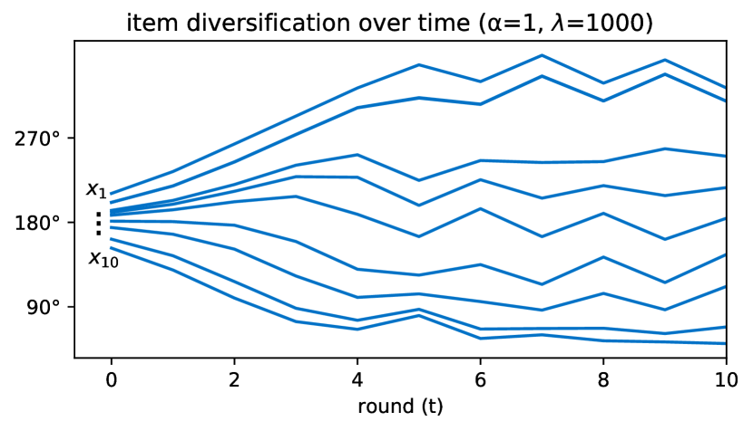
Figure 3: Dispersal of items $x_{i}\in{\mathbb{R}}^{2}$ over time.

5.2 The role of variation in true user preferences

When learning aims primarily for accuracy, training encourages each $u_{i}$ to be oriented towards its $u^{*}_{i}$. For diversity, this acts as a constraint which restricts the capacity of $f$ to diversify. Here we study the role of variation in $u^{*}_{i}$ as a mediator in this process. Figure 2 (center) shows NDCG (bottom) and diversity (top), both in absolute values and relative to pre-update diversity, for varying $\sigma_{u^{*}}$ and for a range of $\lambda$. Here we sample edges uniformly, and consider a single time step with $\alpha=0$. Without regularization ($\lambda=0$), strategic updates cause diversity to drop to zero, even when user preferences are reasonably dispersed ($\sigma_{u^{*}}=1$). However, even mild regularization ($\lambda=0.05$) suffices for obtaining significant diversity through incentivization, which becomes more pronounced as $\lambda$ grows; for all $\lambda>0.1$, diversity is high, and in effect remains fixed. This suggests our model can effectively utilize natural variation in user preferences. Increased diversity comes at the cost of NDCG, but this diminishes quickly for larger dispersion.

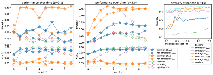
Figure 4: Experiments on Yelp data. (Left+center) Diversity and NDCG over rounds for different methods and target NDCG values, for loose ($\alpha=0.1$; left) vs. restricted ($\alpha=2.0$; center) strategic updates. Our strategic approach consistently achieves significant and sustained improvement in diversity, with minimal loss in accuracy. Right Diversity after $T=10$ rounds for increasing costs scales $\alpha$.

5.3 The role of time vs. modification costs

We now turn to examining the temporal formation of diversity through retraining dynamics, as mediated by modification costs $\alpha$. When $\alpha$ is large, content creators can only apply small changes to $x$ at each round (and vice versa for small $\alpha$). On the one hand, small steps suggest that diversity may require time to form; but on the other, note that small steps also allow the system to intervene with high fidelity and direct incentives throughout, and hence to gradually ‘steer’ behavior towards diversification. Figure 2 (right) shows diversity (top) and NDCG (bottom) for increasing $\alpha$ and over multiple retraining rounds. We set $\lambda$ to be large so that learning is geared primarily towards diversity. When $\alpha$ is small (here, $<1$), diversity quickly drops to zero—as in Prop. 1. In contrast, $\alpha=1$ exhibits a sharp transition, in which diversity quickly rises. Fig. 3 visualizes for a set of items in ${\mathbb{R}}^{2}$ how they quickly become dispersed. Larger $\alpha$ entail similarly high diversity: here the process is slower—since update steps are smaller, but also more stable—since the system has finer control over each step; c.f. $\alpha=1$, where NDCG fluctuates.

6 Experiments on Real Data

We now turn to evaluating our approach on real data. Here we study how NDCG and diversity evolve over time under different learning methods and experimental conditions. See Appendix D for additional details, and Appendix E for extended results (E.1,E.2), a sensitivity analysis to misspecification of $\alpha$ (E.3), and additional similarity metrics (E.4).

Data.

Our experimental setup is based on the restaurants portion of the Yelp dataset, which includes user-submitted restaurant reviews. We focus on users having at least 100 reviewed restaurants. For each user $i$, we construct the list of potential items $X_{i}$ to include the 40 most popular restaurants of those reviewed by $i$, which amounts to 236 users and 1,520 restaurants in total. We elicit $d=43$ restaurant features (e.g., cuisine type, noise level) to be used by the system for learning. We also elicit ‘ground truth’ user features $u^{*}_{i}$ used for optimizing $f^{*}(x^{\prime},u^{*}_{i})$, which is trained to predict the likelihood that $i$ will review $x$, interpreted here as relevance $y$. The labeling function $f^{*}$ is used only for determining updated relevancies $y^{\prime}$ for modified items $x^{\prime}$; neither $f^{*}$ nor the $u^{*}_{i}$ are known to the learner. We ensure $f^{*}$ is distinct from learnable functions $f$ by several means: (i) $f^{*}$ is a fully-connected deep network, whereas $f$ are linear; (ii) $f^{*}$ is trained using true user features $u^{*}_{i}$, which are unobserved for $f$; (iii) $f^{*}$ is trained on considerably more data, and of which the data used for training $f$ is a non-representative subset; and (iv) $f$ is trained on labels that are modified to emphasize highly-rated items. Full details in Appendix D.2.

Setup and learning.

We consider top-10 recommendation (i.e., $k=10$), and evaluate performance over $T=10$ rounds of retraining and corresponding strategic updates. For training, we assume that at each round the system has access to 30 items per user, randomly selected (out of the 40) per round; of these, a random 20 are used for training, and the remaining 10 are added for validation (tuning $\lambda$ and early stopping). Test performance is evaluated on all 40 items. Since the test set includes additional items (compared to training), $f$ must learn to generalize well to new content at each step. Since adding items also changes the graph, and since the graph determines strategic responses—$f$ must also learn to generalize to new forms of strategic updates.

Methods and evaluation.

In line with our dynamic setup (Sec. 2.2), all methods considered aim primarily at optimizing ‘current’ NDCG (i.e., at time $t$ maximize NDCG on $x^{(t)}$), but differ in how (and if) they promote diversity. These include: (i) a non-strategic approach which regularizes for current diversity on non-strategic inputs $x^{(t)}$ (Eq. (7)), (ii) our strategic approach, which regularizes for future diversity on the anticipated $x^{(t+1)}=x^{f_{t}}$ (Eq. (10)), (iii) an accuracy-only baseline, which does not promote diversity (by setting $\lambda=0$), (iv) re-ranking using the popular MMR diversification procedure (Carbonell & Goldstein, 1998), and (v) a hybrid@$t$ approach, which runs strategic for $t=5$ rounds, and then ‘turns off’ regularization.

Since non-strategic and strategic are designed to balance NDCG and diversity, for a meaningful comparison, in each experimental condition we fix a predetermined target value for NDCG, tune each method at each round to achieve this target (using $\lambda$, on the validation set, and up to tolerance 0.01), and compare the resulting diversity. We use the notation $\lambda_{\beta}$ to mean that $\lambda$ was tuned for the target $\beta$. To compare with baseline, in one condition we set $\lambda$ to the largest value that maintains the same NDCG as the baseline (for which $\lambda=0$), denoted $\lambda_{\text{base}}$.Note that due to performativity, data at time $t$ depends on the learned model at time $t-1$. Because our dynamics are stateful, results are path-dependent, and so comparisons must be made across full trajectories—and cannot be made independently at each time point.

6.1 Diversity over time

Our first experiment studies how diversity evolves over time for different NDCG targets. Fig. 4 (left) shows diversity (top) and NDCG (bottom) per round for $\alpha=0.1$, which permits significant (yet restricted) strategic updates. Results show that for baseline, which does not actively promote diversity, average diversity decreases over time by roughly 40%. Adding MMR, which re-ranks for diversity, improves only marginally. In the $\lambda_{\text{base}}$ condition, diversity for non-strategic improves only slightly compared to baseline, mostly at the onset. In contrast, our strategic approach is able to consistently maintain (and even slightly increase) diversity over time, albeit at small occasional drops in test NDCG, as compared to non-strategic ($\leq 0.02$). In the $\lambda_{0.9}$ condition, non-strategic is able to preserve roughly 80% of diversity by sacrificing $\sim 13\%$ of the optimal NDCG. Meanwhile, and for the same loss in NDCG, strategic is able to quickly double the initial diversity—and sustain it, likely through means similar to those observed in Sec. 5.3. Note that sustaining diversity requires to actively promote it throughout; once regularization is switched off (hybrid), diversity immediately drops.

Fig. 4 (center) shows results for a similar setting, but using a larger $\alpha=2$. In comparison, here diversity for all methods improves—but for baseline and MMR, this is only transient. Results are also smoother, and accumulate—for both improvement and deterioration—which is likely due to the fact that strategic movements are now more restricted. The biggest distinction here is that for $\lambda_{0.9}$, non-strategic eventually obtains the same level of diversity as strategic, this likely due to $\alpha$ being large: small updates mean that $x$ and $x^{f}$ are correlated, and so regularizing for $\operatorname{div}(X,{\bm{r}})$ also improves $\operatorname{div}(X^{f},{\bm{r}}^{f})$ to some extent. Here the advantage of strategic is that it improves much faster.

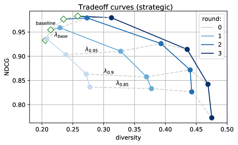
Figure 5: Pareto curves for strategic, per round (solid lines) and per $\lambda$ (dashed).

6.2 The role of modification costs.

To further examine the role of $\alpha$, we compare performance across a range of cost scales and for multiple target NDCG values. Fig. 4 (right) shows diversity at $T=10$. As can be seen, all methods benefit from increasing $\alpha$. However, diversity for baseline remains below that of a random baseline which recommends $k$ random items. For strategic, sacrificing fairly little NDCG ($\lambda_{0.95}$ and below) suffices for gaining significant diversity across all $\alpha$. Results also show how $\alpha$ mediates the gap between non-strategic and strategic, which increases as $\alpha$ grows.

6.3 Tradeoffs over time.

Fig. 5 shows Pareto curves for strategic, obtained by considering multiple $\lambda$ and over several rounds. Results show that the entire tradeoff curve between NDCG and diversity improves over time. Paths for each target NDCG depict specific trajectories, and show how diversity can be created without sacrificing accuracy. This holds even when no compromise in accuracy is allowed: even though both baseline and $\lambda_{\text{base}}$ maximize accuracy, our strategic approach is able to steer content creators towards more diverse content. This is achieved by utilizing the flexibility to choose $u_{i}$ which improve both accuracy and diversity.

7 Discussion

Through the lens of performativity, our paper studies how a learning system can incentivize content creators to collectively form a more diverse inventory of items for recommendation. In this, we challenge the conventional view that diversity is merely a matter of which items to present (and which not), and argue that to fundamentally rectify the predisposition of modern recommendation systems to homogenize content, learning must (i) recognize that content changes over time, in part due to the strategic behavior of content creators, and (ii) capitalize on its power shape incentives and steer towards diversity. Our work joins others in taking a step towards studying recommendation systems as complex ecosystems in which users, creators, and the system itself act and react to promote their own goals and aspirations. From a learning perspective, this requires us to rethink the role that predictions play in the recommendation process, and consider its implications on user welfare.

Acknowledgements

This research was supported by the Israel Science Foundation (grant No. 278/22) and by VATAT Fund to the Technion Artificial Intelligence Hub (Tech.AI).

Appendix A Optimization

A.1 Closed form expression for best response $\Delta_{f}$

Proof.

To compute an item’s best-response update $\Delta_{f}(x)$, we must solve the following constrained problem:

$$\max_{x^{\prime}}v^{T}x^{\prime}-\alpha c(x^{\prime},x)\quad\textrm{s.t}\quad||x||_{2}=1$$

where $$c(x,x^{\prime})=\|x^{\prime}-x\|_{2}^{2} x^{\prime}$$. We solve for using Lagrangian analysis. First, we square the constraint (which does not change the condition itself). Define the Lagrangian as follows:

$$L(x^{\prime},\lambda)=v^{T}x^{\prime}-\alpha\|x^{\prime}-x\|_{2}^{2}+\lambda[||x^{\prime}||_{2}^{2}-1]$$

Next, to find the minimum of $$L x^{\prime}$$, derive with respect to , and compare to 0:

$$v-2\alpha(x^{\prime}-x)+2\lambda x^{\prime}=0$$

$$v+2\alpha x=2\alpha x^{\prime}-2\lambda x^{\prime}$$

$$\frac{v+2\alpha x}{2\alpha-2\lambda}=x^{\prime}$$

Plugging $$x^{\prime}$$ into the original constraint gives:

$$\frac{|v+2\alpha x|}{|2\alpha-2\lambda|}=1$$

$$|v+2\alpha x|=2\alpha-2\lambda$$

$$|v+2\alpha x|-2\alpha=-2\lambda$$

Finally, plugging $$\lambda x^{\prime}_{i}$$ into the expression for obtains:

$$\frac{v+2\alpha x}{|v+2\alpha x|}=x^{\prime}$$

Appendix B Proofs

B.1 Proposition 1

Proof.

As both items have the same set of users, the normalized average of user embeddings is the same for both items, i.e., ${\tilde{v}}_{1}={\tilde{v}}_{2}={\tilde{v}}$. Since $\alpha=0$, the best response (Eq. (11)) is given by $\Delta_{f}(x_{j})={\tilde{v}}$ for both $j=1,2$. Hence, both items are modified in the same way, and so diversity is by definition zero. ∎

B.2 Proposition 2

We begin with a useful lemma.

Lemma 4.

For any $n>1$ there exists a set of $n$ unit-norm user embeddings $U=\{u_{1},\dots,u_{n}\}$ for which:

$$\sum_{u_{i}\in U}u_{i}=\overrightarrow{0}$$

where $\overrightarrow{0}$ is the zero vector.

Proof.

We prove for $d=2$; for $d>2$, we set the first two coordinates accordingly, and the other $d-2$ coordinates are set to zero. For $n=2$, we define $U_{2}=\{u_{1},u_{2}\}$ as follows:

$$u_{1}=(-1,0),\quad u_{2}=(1,0)$$

Note that indeed $\sum_{u_{i}\in U_{2}}u_{i}=u_{1}+u_{2}=(0,0)$.

For $n=3$, we define $U_{3}=\{u_{1},u_{2},u_{3}\}$ as follows:

$$u_{1}=(\frac{1}{2},\frac{\sqrt{3}}{2}),\quad u_{2}=(\frac{1}{2},-\frac{\sqrt{3}}{2}),\quad u_{3}=(-1,0)$$

Here as well $\sum_{u_{i}\in U_{3}}u_{i}=u_{1}+u_{2}+u_{3}=(0,0)$.

Observation: $\forall n>1$ $\exists a,b\geq 0$ for which $n=2a+3b$.

Thus, for any $n>1$, we define $U$ to include $a$ copies of $U_{2}$ and $b$ copies of $U_{3}$. Using this construction, we get $\sum_{u_{i}\in U}u_{i}=(0,0)$, as required. ∎

We now return to proving the proposition. The general idea is to define two embeddings that are maximally distinct, and ensure all others do not interfere with their orientation.

Proof.

First we prove that for $|U|>1$ diversity is one. According to Lemma 4, there exists a set of user embedding vectors $U$ of size $|U_{1}\bigcap U_{2}|$ that holds:

$$\sum_{u\in U}u=\overrightarrow{0}$$

We define an $f$ that assigns to each user in $|U_{1}\bigcap U_{2}|$ a vector in $U$ (one to one map). Since the sum of the vectors in $U$ is 0 it holds that ${\tilde{v}}_{1}=u_{1}$ and ${\tilde{v}}_{2}=u_{2}$. Since $\alpha=0$, there are no modification costs, and the strategic response of items according to Eq. (11) is $\Delta_{f}(x_{1})=u_{1}$ and $\Delta_{f}(x_{2})=u_{2}$. In order to create maximal diversity between $\Delta_{f}(x_{1})$ and $\Delta_{f}(x_{2})$, we can use any choice of vectors $u_{1}$ and $u_{2}$ that satisfy $u_{1}=-u_{2}$.
∎

B.3 Proposition 3

We prove for $d=2$; for $d>2$, we set the first two coordinates accordingly, and the other $d-2$ coordinates are set to zero. This allows us to work with angles between user embeddings $u$. We use ‘x’ and ‘y’ to refer to the corresponding Cartesian components of angles.

Consider the following graph and user vector embeddings. For each $i<N$, define user $i$’s list of candidate items $X_{i}$ to include the items $x_{i},x_{i+1}$. For user $N$, the items in $X_{N}$ are $x_{N},x_{1}$.

Let $0<\delta$. Define the following embedding: For every odd $i<N$, set $u_{i}=90-i\delta$; For every even $i<N$, set $u_{i}=270-i\delta$. For $i=N$ we define $u_{N}=270+\delta$. Note that this gives $x_{1}=(1,0)$ since the two users that influence $x_{1}$ are $u_{1}$ and $u_{N}$, whose average gives a vector with coordinates:

$$\text{x}:\quad \frac{1}{2}(cos(270+\delta)+cos(90-\delta))=$$

$$\frac{1}{2}(cos(-90+\delta)+cos(90-\delta))=$$

$$\frac{1}{2}(cos(-(90-\delta)+cos(90-\delta))=$$

$$\frac{1}{2}(cos((90-\delta)+cos(90-\delta))=$$

$$cos(90-\delta)$$

$$\text{y}:\quad \frac{1}{2}(sin(270+\delta)+sin(90-\delta))=$$

$$\frac{1}{2}(sin(-90+\delta)+sin(90-\delta))=$$

$$\frac{1}{2}(-sin(90-\delta)+sin(90-\delta))=$$

$$=0$$

This item’s y value is 0; hence, do due unit norm constraints, we have $x_{1}=(1,0)$.

We now calculate the response of $x_{i}$ when $i$ is even for all $1<i<N$. The users associated with $x_{i}$ are:

$$u_{i-1}=90-(i-1)\delta,\qquad u_{i}=270-i\delta$$

We average the two vectors by averaging each coordinate $x,y$:

$$\text{x}:\quad \frac{1}{2}(cos(270-i\delta)+cos(90-(i-1)\delta))=$$

$$cos(\frac{360-(2i-1)\delta}{2})cos(\frac{180-\delta}{2})=$$

$$cos(180-\frac{2i-1}{2}\delta)cos(90-\frac{\delta}{2})=$$

$$-cos(\frac{2i-1}{2}\delta)sin(\frac{\delta}{2})$$

$$\text{y}:\quad \frac{1}{2}(sin(270-i\delta)+sin(90-(i-1)\delta)=$$

$$sin(\frac{360-(2i-1)\delta}{2})cos(\frac{180-\delta}{2})=$$

$$sin(180-\frac{2i-1}{2}\delta)cos(90-\frac{\delta}{2})=$$

$$sin(\frac{2i-1}{2}\delta)sin(\frac{\delta}{2})$$

Normalizing gives:

$$\sqrt{(-cos(\frac{2i-1}{2}\delta)sin(\frac{\delta}{2}))^{2}+(sin(\frac{2i-1}{2}\delta)sin(\frac{\delta}{2}))^{2}}=sin(\frac{\delta}{2})\sqrt{cos(\frac{2i-1}{2}\delta)^{2}+sin(\frac{2i-1}{2}\delta)^{2}}=sin(\frac{\delta}{2})$$

Note this must be positive since it describes a vector length; since $0<\delta<180$, this length is $sin(\frac{\delta}{2})$ (and not $-sin(\frac{\delta}{2})$). The normalized vector is:

$$(-cos(\frac{2i-1}{2}\delta),sin(\frac{2i-1}{2}\delta))=(cos(180-\frac{2i-1}{2}\delta),sin(180-\frac{2i-1}{2}\delta))$$

Since $\alpha=0$, according to Eq. (11),this gives $\Delta(x_{i})$.

Next, we calculate the response of $x_{i}$ when $i$ is odd for all $1<i<N$. The users associated with $x_{i}$ are:

$$u_{i-1}=270-(i-1)\delta$$

$$u_{i}=90-i\delta$$

We average the two vectors by averaging each coordinate $x,y$:

$$\text{x}:\quad \frac{1}{2}(cos(270-(i-1)\delta)+cos(90-i\delta)=$$

$$cos(\frac{360+(1-2i)\delta}{2})cos(\frac{180+\delta}{2})=$$

$$cos(180-\frac{2i-1}{2}\delta)cos(90+\frac{\delta}{2})=$$

$$cos(\frac{2i-1}{2}\delta)sin(\frac{\delta}{2})$$

$$\text{y}:\quad \frac{1}{2}(sin(270-(i-1)\delta)+sin(90-i\delta)=$$

$$sin(\frac{360-(2i-1)\delta}{2})cos(\frac{180+\delta}{2})=$$

$$sin(180-\frac{2i-1}{2}\delta)sin(-\frac{\delta}{2})=$$

$$-sin(\frac{2i-1}{2}\delta)sin(\frac{\delta}{2})$$

Normalizing gives:

$$\sqrt{(cos(\frac{2i-1}{2}\delta)sin(\frac{\delta}{2}))^{2}+(-sin(\frac{2i-1}{2}\delta)sin(\frac{\delta}{2}))^{2}}=sin(\frac{\delta}{2})\sqrt{cos(\frac{2i-1}{2}\delta)^{2}+sin(\frac{2i-1}{2}\delta)^{2}}=sin(\frac{\delta}{2})$$

The normalized vector is:

$$(cos(\frac{2i-1}{2}\delta),-sin(\frac{2i-1}{2}\delta))=(cos(-\frac{2i-1}{2}\delta),sin(-\frac{2i-1}{2}\delta))$$

Since $\alpha=0$, according to Eq. (11),this gives $\Delta(x_{i})$.

We now calculate the diversity for each user $i<N-1$. User $i=1$ has items $x_{1}$ and $x_{2}$ in his list. Thus, diversity is:

$$\frac{1-x_{1}^{T}x_{2}}{2}=\frac{1}{2}(1-(1\cdot(-cos(\frac{4-1}{2}\delta)+0\cdot sin(\frac{4-1}{2}\delta)))=\frac{1+cos(\frac{3\delta}{2})}{2}$$

For even $i$, we first calculate the cosine similarity:

$$x_{i}^{T}x_{i+1}=$$

$$-cos(\frac{2i-1}{2}\delta)cos(-\frac{2(i+1)-1}{2}\delta)+sin(\frac{2i-1}{2}\delta)sin(-\frac{2(i+1)-1}{2}\delta)=$$

$$-cos(\frac{2i-1}{2}\delta)cos(-\frac{2i+1}{2}\delta)+sin(\frac{2i-1}{2}\delta)sin(-\frac{2i+1}{2}\delta)=$$

$$-[cos(\frac{2i-1}{2}\delta)cos(-\frac{2i+1}{2}\delta)-sin(\frac{2i-1}{2}\delta)sin(-\frac{2i+1}{2}\delta)]=$$

$$-cos(\frac{2i-1}{2}\delta-\frac{2i+1}{2}\delta)=$$

$$-cos(\delta)$$

Diversity is given by:

$$\frac{1-x_{i}^{T}x_{i-1}}{2}=\frac{1+cos(\delta)}{2}$$

For odd $i$, cosine similarity is:

$$x_{i}^{T}x_{i+1}=$$

$$-cos(-\frac{2i-1}{2}\delta)cos(\frac{2(i+1)-1}{2}\delta)+sin(-\frac{2i-1}{2}\delta)sin(\frac{2(i+1)-1}{2}\delta)=$$

$$-cos(-\frac{2i-1}{2}\delta)cos(\frac{2i+1}{2}\delta)+sin(-\frac{2i-1}{2}\delta)sin(\frac{2i+1}{2}\delta)=$$

$$-[cos(-\frac{2i-1}{2}\delta)cos(\frac{2i+1}{2}\delta)-sin(-\frac{2i-1}{2}\delta)sin(\frac{2i+1}{2}\delta)]=$$

$$-cos(-\frac{2i-1}{2}\delta+\frac{2i+1}{2}\delta)=$$

$$-cos(\delta)$$

Diversity is given by:

$$\frac{1-x_{i}^{T}x_{i-1}}{2}=\frac{1+cos(\delta)}{2}$$

We have remaining diversity for users $N-1$ and $N$. Denote their corresponding diversities by $d_{N-1}$ and $d_{N}$. The overall average diversity (Eq. (4)) is:

$$\operatorname{div}=\frac{1}{N}\left(d_{N-1}+d_{N}+\frac{1+cos(\frac{3\delta}{2})}{2}+\frac{(N-3)(1+cos(\delta))}{2}\right)$$

Since $d_{N-1}$ and $d_{N}$ are non-negative, we get:

$$\operatorname{div}\geq\frac{1}{N}\left(\frac{1+cos(\frac{3\delta}{2})}{2}+\frac{(N-3)(1+cos(\delta))}{2}\right)$$

Note $\frac{1+cos(\frac{3\delta}{2})}{2}$ is also non-negative since $cos(\frac{3\delta}{2})$ cannot be less than $-1$. Hence, we get:

$$\operatorname{div}\geq\frac{(N-3)(1+cos(\delta))}{2N}=\frac{N-3}{N}\frac{1+cos(\delta)}{2}$$

Finally, set $\delta=cos^{-1}(1-2\epsilon)$; this gives $\epsilon=\frac{1-cos(\delta)}{2}$, and since $1-\epsilon=\frac{1+cos(\delta)}{2}$, we get as required:

$$\operatorname{div}\geq\left(1-\frac{3}{N}\right)(1-\epsilon)$$

∎

Appendix C Additional Experimental Results: Synthetic Data

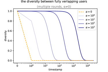
Figure 6: Empirical generalization of Proposition 1 for $\alpha\neq 0$.

C.1 Empirical analysis: Proposition 1 beyond $\alpha=0$

Proposition 1 states that full user overlap leads to zero diversity, but relies on the assumption that $\alpha=0$, i.e., that there are no modification costs, and so items can move arbitrarily on the unit sphere. Our motivation for considering $\alpha=0$ (and a single time step) was that it is a useful proxy for larger $\alpha$ over multiple updates (that do not include retraining). Here we demonstrate empirically that this is indeed the case, i.e., that for $\alpha>0$, diversity does go to zero over time.

We consider two items, positioned so that they are as far apart as possible: $x_{1}=(1,0)$ and the other at $x_{2}=(-1,0)$. We set ${\tilde{v}}$, which represents the spherical average of the overlapping users, to a random direction. We then measure how diversity changes over the time. As shown in Figure 6 diversity drops to zero for all $\alpha$ considered.

C.2 Accuracy and diversity over time

As an intermediate step between the experiments in Sec. 5.2 and Sec. 5.3, here we consider how accuracy and diversity trade off over time and for a range of $\lambda$, but while keeping $\alpha=0$. Results are shown in Figure 7. For $\lambda=0$ (i.e., learning does not regularize for diversity), resulting NDCG is high and fixed, but diversity is nearly zero. This can be explained by the small value of $\sigma_{u^{*}}$, which implies that after strategic modification, items will be highly similar—which eliminates diversity (as in experiment 5.2), and makes the ranking task easy (since all items are similarly relevant). In the other extreme, when $\lambda=1000$ (and so diversity is heavily regularized for), we observe that in the first round, diversity increases sharply, whereas NDCG decreases. In the subsequent rounds, diversity remains high and NDCG remains low.

For intermediary $\lambda$, results show how the learning allows to balance NDCG and diversity, where diversity is obtained for little loss in NDCG. For larger $\lambda$, more NDCG is sacrificed and diversity increases. An interesting phenomena is that lower values of $\lambda$ exhibit periodic behavior. For example, for $\lambda=0.025$, diversity alternates between very high (even round) and very low (odd rounds). Given how NDCG and diversity relate, we see two possible explanations for this:

1. When diversity is high, the relevance of items may differ significantly. As a result, even a mild change in the item’s ranking can cause NDCG to drop. To avoid this loss of NDCG, one solution is for the model to learn user embeddings $u_{i}$ that are close to $u^{*}$. This, however, causes diversity to be low in the next round.

2. When diversity is low, item features are very similar, and hence have highly similar relevance values. This implies that most rankings will have similar NDCG. Consequently, learning can encourage diversity without sacrificing current NDCG.

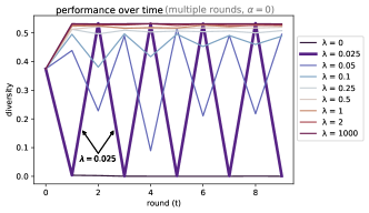
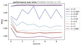
Figure 7: (Left) diversity vs number of rounds. (Right) NDCG vs number of rounds.

C.3 The role of the number of recommended items $k$

Here we consider how the size of the recommendation list $k$ impacts the ability of the model to create diversity. We keep all other aspects of the experiment fixed, and vary $k$. Figure 8 shows results for two values of $\lambda$: a low (but positive) value of $\lambda=0.025$ (left), and a high value of $\lambda=1$. Overall, results show that higher $k$ enables larger diversity; conversely, when $k$ is small, results show that it is harder for the model to encourage diversity. One possible reason is that due to linearity, the top of the list is likely to includes items that are similar. The main distinction between the low and high $\lambda$ is how diversity appears over time. As in the previous experiment in Sec. C.2 (in which $k=10$), we see that $\lambda=0.025$ exhibits alternating diversity for all $k$. For $\lambda=1$, lower $k$ still exhibits some fluctuations, but these become small as $k$ grows.

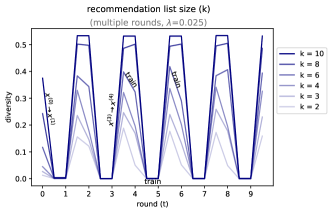
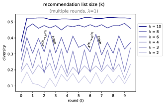
Figure 8: (Left) diversity vs number of rounds for $\lambda=0.025$. (Right) diversity vs number of rounds for $\lambda=1$.

Appendix D Experimental details

D.1 Data

Our experiments use the Yelp dataset, which is publicly available at https://www.yelp.com/dataset/download.

Items.

Yelp includes data about many business types; of these, our experiment focuses on restaurants. To obtain restaurant entries, we manually identify and select all categories that pertain to restaurants (e.g, ‘pizzaria’ or ‘burger bar’). This results in 22,197 distinct entries.

Features.

For features, we use a subset of the available features that were prevalent, and which were found to be informative for training $f^{*}$. We use category information to form additional features by grouping similar categories having similar contextual meaning; for example, the categories ‘pizza’, ‘pasta’, ‘calzone’, etc. are assigned the binary feature ‘Italian cuisine’. Overall we use 43 features, which include:

’stars’, ’alcohol’, ’restaurants good for groups’, ’restaurants reservations’, ’restaurants attire’, ’bike parking’, ’restaurants price range’, ’has tv’, ’noise level’, ’restaurants take out’, ’caters’, ’outdoor seating’, ’good for meal-dessert’, ’good for meal-late night’, ’good for meal-lunch’, ’good for meal-dinner’, ’good for meal-brunch’, ’good for meal-breakfast’, ’dogs allowed’, ’restaurants delivery’, ’japanese’, ’chinese’, ’india’, ’middle east’, ’mexican food’, ’sweets’, ’coffee’, ’italian’, ’burgers’, ’hot dogs’, ’sandwiches’, ’steak’, ’pizza’, ’seafood’, ’fast food’, ’vegan’, ’ice cream’, ’restaurants table service’, ’business accepts credit cards’, ’wheel chair accessible’, ’drive thru’, ’happy hour’, ’corkage’.

Users.

As noted, we focus on active users who have contributed at least 100 reviews. One reason is that we have found that including low-activity users in this dataset results in a sparse and disconnected graph, with many isolated items (and corresponding users); this trivializes the task of diversification since most items can be incentivized independently. For each user, we consider the 40 most popular items (of those rated by that user), since by similar reasoning these provide larger overlap, and hence more intricate dependencies across items. In particular, we use the following procedure to construct potential item lists:

Denote by $R$ the set of all restaurants, and by $U$ set of active users.

• for all users $u\in U$, initialize $X_{u}=\emptyset$

• for all restaurants $r\in R$, initialize $U_{r}$ to include all users $u$ that have reviewed restaurant $r$

• while exists $u\in U$ for which $|X_{u}|<40$:

  • let $r$ be the restaurant with the most users in $U$, i.e., $U_{r}\cap U$ is largest

  • for each user $u\in U_{r}$:

    • add $r$ to $X_{u}$

    • remove $r$ from $R$

    • if $|X_{u}|=40$, then for each $r^{\prime}$ in $x_{u}$, remove $u$ from $U_{r^{\prime}}$

D.2 Generating counterfactual ground-truth labels (pre-processing)

Since our experiments include modified items $x^{f}_{j}$ that do not exist in the data, for learning and evaluation we require means to generate corresponding counterfactual relevance scores $y^{f}_{j}$. To achieve this, prior to the experiment we train a ground truth labeling function, $f^{*}(x)$, which we query for updated labels throughout the experiment. As noted, we ensure $f^{*}$ is distinct from (and more powerful than) the predictive models $f$ we learn in the actual experiment.

Data for training $f^{*}$.

We train $f^{*}$ on all data generated by users having at least 50 restaurant reviews; these amount to 1,377 users and 113,852 reviews. Since the original data does not include informative user features, we generate ground-truth user features $u^{*}_{i}$ by aggregating for each user $i$ the features of all restaurants reviewed by $i$. This is similar in spirit to approaches for content-based recommendation. Formally, we define $u_{i}^{*}=\frac{1}{{|\operatorname{rev}_{i}|}}\sum_{x\in\operatorname{rev}_{i}}x$, where $\operatorname{rev}_{i}$ is the set of all restaurants that the user $i$ reviewed.

For labels, we consider probabilistic labels $y_{ij}\in[0,1]$ that describe the likelihood that user $i$ will visit restaurant $j$, which we interpret as relevance. For each user $i$, we set $y_{ij}=1$ for every restaurant $j$ that $i$ reviewed. To obtain negative labels, for each $(i,j)$ pair, we first obtain the geographical location of restaurants $j$, and then retrieve the closest restaurant $j^{\prime}$ (in geographical terms) to $j$ that $i$ did not review; we then set $y_{ij^{\prime}}=0$. This is intended to mimic a setting in which $i$ could have went to either $j$ or $j^{\prime}$ (since they are physically nearby), but chose to go to $j$.

Architecture.

We set $f^{*}$ to be an MLP with ReLU activations. We use five layers, which we have found to be sufficient for expressing the non-linear relations between user and item features found in the data. The first layer has 86 inputs (43 restaurant features and 43 user features) and $86\times 2=172$ outputs, and for each consecutive layer the output dimension reduces by half.

Training and evaluation.

We split the data into train, validation, and test sets, using a 70-20-10 split. We optimize using Adam with a learning rate of 0.01, which gives a reasonable balance between performance and runtime, and used the validation set for early stopping. The final $f^{*}$ achieves 72% accuracy on the held-out test set.

D.3 Hyper-parameters and tuning (main experiment)

For optimizing predictive models $f$ in each experimental condition, we use Adam and train for a maximum of 200 epochs with learning rate 0.1. For smoothing (see Sec. 3.1), we use temperatures $\tau=0.1$ for NDCG, $\tau=1$ for the permutation matrix approximation, and $\tau=5$ for the soft-$k$ function; all were chosen to be the largest feasible values that permit smooth training. All experiments were run on a cluster of AMD EPYC 7713 machines (1.6 Ghz, 256M, 128 cores).

Appendix E Additional experimental results: real data

E.1 Diversity over time – additional results

Figure 9 includes extended results pertaining to our main experiment in Sec. 6.1 for additional cost scales $\alpha$.

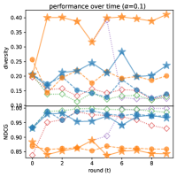
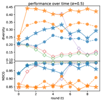
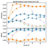
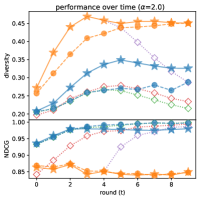
Figure 9: Diversity and NDCG over rounds for different methods and target NDCG values, and for costs $\alpha\in\{0.1,0.5,1,2\}$.

E.2 Tradeoffs over time – additional results

Figure 10 includes extended results for our experiment on tradeoffs over time in Sec. 6.2 for additional cost scales $\alpha$.

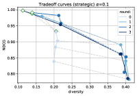
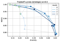
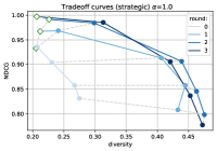
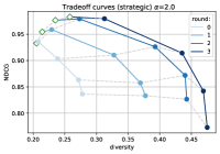
Figure 10: Pareto curves for strategic per round (varying $\lambda$; solid lines), and vs. baseline. Dashed lines show per-$\lambda$ trajectories.

E.3 Sensitivity to a misspecification of the response model

Our experiments in Sec. 6 consider a setting in which the system has knowledge of the response model $\Delta$, and in particular, of the true cost scale $\alpha$. In this section we explore the sensitivity of our approach to learning under misspecified $\alpha$. In particular, in each experimental instance, we train our model on some $\alpha$, but test it on a different $\alpha^{\prime}$. Note that the misspecified $\alpha$ is used throughout all training rounds, and so the effects of misspecification accumulate.

Figure 11 (left) shows diversity over rounds on a fixed test $\alpha=1$, for smaller training $\alpha\in[0.6,1)$ (blue lines), larger training $\alpha\in(1,1.4]$ (red lines), and the correct training $\alpha=1$ (black line). Results show our approach is fairly robust to misspecification, with performance for all train $\alpha$ almost matching the correct one. Figure 11 (right) shows similar results for test $\alpha=0.5$. Here robustness is preserved in full for smaller $\alpha\in[0.1,0.5)$, but shows some deterioration in performance for the larger $\alpha\in(1,1.4]$.

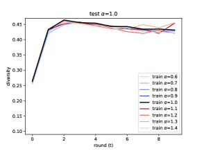
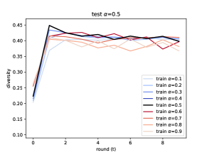
Figure 11: Diversity for misspecified cost scale $\alpha$, for fixed test $\alpha$ and varying train $\alpha$.

Complementarily, Figure 12 shows diversity for fixed train $\alpha$ and varying test $\alpha$. Here, performance is again robust for $\alpha=1$ (left). However, for the smaller train $\alpha=0.5$ (right), in which items are subject to more dramatic modifications, mispecification has a significant effect on performance. For smaller test $\alpha$ (blue lines), sever overestimation of $\alpha$ in training (e.g., 0.5 vs. test $\alpha=0.1$) has a severe negative effect on diversity over time. Interestingly, underestimation of $\alpha$ in training (red lines) results in improved diversity, suggesting that perhaps taking excessive cautionary steps is helpful in this case.

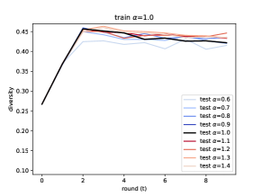
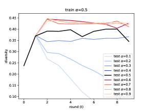
Figure 12: Diversity for misspecified cost scale $\alpha$, for fixed train $\alpha$ and varying test $\alpha$.

E.4 Entropy-based diversity regularization

As we state in Sec. 2, our paper focuses predominantly on cosine similarity, which we believe is appropriate for the recommendation environment we consider, and is a popular choice in the literature. Nonetheless, our approach is not restricted to this choice, and in this section we describe how it can be extended to operate on other similarity measures, and in particular, on entroty-based similarity. We then provide some empirical results for this settings.

To begin, note that conventional entropy regularization (e.g., Qin & Zhu (2013)) assumes a Gaussian distribution over feature vectors, and so is not immediately applicable to our setting of unit-norm features. To account for this, we propose a similar measure, but based on the Beta distribution, which is appropriate for inputs in [0,1], and which can apply per feature. The benefits of this measure are that: (i) its parameters can be efficiently estimated using moment matching (Owen, 2008); (ii) both parameter estimates and the differential entropy function are differentiable, and hence permit gradients to pass through; and (iii) entropy can be made to take strategically-modified inputs, and hence allow for strategically-aware optimization.

The Beta distribution is defined by two shape parameters, $a>0$ and $b>0$. Let $Z\sim\textrm{Beta}(a,b)$, and for a given sample of such $Z$-s, denote its average by $\bar{Z}$ its standard deviation by $S$. Then the parameters $a$ and $b$ can be efficiently estimated as:

$$\hat{a}=\bar{Z}(\bar{Z}\frac{(1-\bar{Z})}{S^{2}}-1),\qquad\qquad\hat{b}=(1-\bar{Z})(\bar{Z}\frac{(1-\bar{Z})}{S^{2}}-1)$$

Our approach is to consider each feature in each item list as deriving from some Beta distribution. Hence, for a given list $X$ and feature $i$, we first estimate $\hat{a},\hat{b}$ using $\{x_{i}\}_{x\in X}$. Note that both estimands are differentiable. Then, we compute entropy for this list and feature as $e_{i}(X)=\textrm{entropy}(\hat{a},\hat{b})$, which admits a differentiable closed form (we used the pytorch implementation that allows to pass gradients). Finally, we define $\operatorname{div}(X)=\frac{1}{d}\sum_{i=1}^{d}e_{i}(X)$. We can then replace $X$ with $X^{f}$, and plug into our objective in Eq. (10), which remains differentiable.

Using this approach, we extend our main experiments to also include entropy-based regularization. Figure 13 shows diversity and NDCG for all methods, when diversity is measured using entropy. Here again we see that strategically-aware methods outperform non-strategic methods across multiple cost scales $\alpha$, although to a lesser extent than when measuring cosine similarity. Interestingly, optimizing for the incorrect correct measure (here, cosine; blue and orange) performs as well as when the correct measure (i.e., entropy; red and green) is optimized.

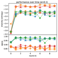
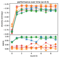
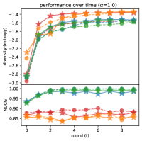
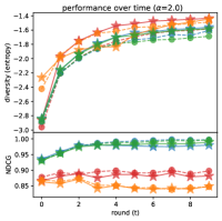
Figure 13: Experiments using entropy-based similarity as a diversity measure.

Finally, we rerun our original experiment using cosine similarity as a measure of diversity, but considering also methods that optimize entropy-based similarity (red and green). Here we see that misspecified diversity regularization is useful, but to a lesser extent than the correct form of regulariztaion. Nonetheless, the importance of awareness to strategic behavior remains to be more important (in terms of performance) than applying the correct regularizer.

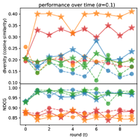
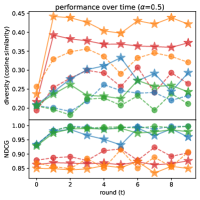
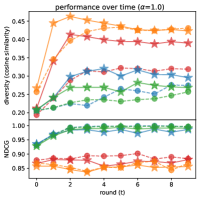
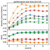
Figure 14: Experiments using cosine similarity as a diversity measure, but including also methods that optimize entropy-based diversity.

References

- Abdollahpouri et al. (2017) Abdollahpouri, H., Burke, R., and Mobasher, B. Controlling popularity bias in learning-to-rank recommendation. In Proceedings of the eleventh ACM conference on recommender systems, pp. 42–46, 2017.
- Abdollahpouri et al. (2019a) Abdollahpouri, H., Burke, R., and Mobasher, B. Managing popularity bias in recommender systems with personalized re-ranking. In The thirty-second international flairs conference, 2019a.
- Abdollahpouri et al. (2019b) Abdollahpouri, H., Mansoury, M., Burke, R., and Mobasher, B. The unfairness of popularity bias in recommendation. arXiv preprint arXiv:1907.13286, 2019b.
- Anderson (2006) Anderson, C. The long tail: Why the future of business is selling less of more. Hachette UK, 2006.
- Antikacioglu et al. (2019) Antikacioglu, A., Bajpai, T., and Ravi, R. A new system-wide diversity measure for recommendations with efficient algorithms. SIAM Journal on Mathematics of Data Science, 1(4):759–779, 2019.
- Bechavod et al. (2022) Bechavod, Y., Podimata, C., Wu, S., and Ziani, J. Information discrepancy in strategic learning. In International Conference on Machine Learning, pp. 1691–1715. PMLR, 2022.
- Ben-Porat & Tennenholtz (2018) Ben-Porat, O. and Tennenholtz, M. A game-theoretic approach to recommendation systems with strategic content providers. Advances in Neural Information Processing Systems, 31, 2018.
- Ben-Porat et al. (2019) Ben-Porat, O., Goren, G., Rosenberg, I., and Tennenholtz, M. From recommendation systems to facility location games. Proceedings of the AAAI Conference on Artificial Intelligence, 33(01):1772–1779, Jul. 2019. doi: 10.1609/aaai.v33i01.33011772. URL https://ojs.aaai.org/index.php/AAAI/article/view/4000.
- Ben-Porat et al. (2020) Ben-Porat, O., Rosenberg, I., and Tennenholtz, M. Content provider dynamics and coordination in recommendation ecosystems. Advances in Neural Information Processing Systems, 33:18931–18941, 2020.
- Bradley & Smyth (2001) Bradley, K. and Smyth, B. Improving recommendation diversity. In Proceedings of the Twelfth Irish Conference on Artificial Intelligence and Cognitive Science, Maynooth, Ireland, volume 85, pp. 141–152. Citeseer, 2001.
- Brown et al. (2022) Brown, G., Hod, S., and Kalemaj, I. Performative prediction in a stateful world. In International Conference on Artificial Intelligence and Statistics, pp. 6045–6061. PMLR, 2022.
- (12) Brown, W. and Agarwal, A. Diversified recommendations for agents with adaptive preferences. In Advances in Neural Information Processing Systems.
- Brückner & Scheffer (2009) Brückner, M. and Scheffer, T. Nash equilibria of static prediction games. In Advances in neural information processing systems, pp. 171–179, 2009.
- Brückner et al. (2012) Brückner, M., Kanzow, C., and Scheffer, T. Static prediction games for adversarial learning problems. The Journal of Machine Learning Research, 13(1):2617–2654, 2012.
- Burke (2017) Burke, R. Multisided fairness for recommendation. arXiv preprint arXiv:1707.00093, 2017.
- Carbonell & Goldstein (1998) Carbonell, J. and Goldstein, J. The use of mmr, diversity-based reranking for reordering documents and producing summaries. In Proceedings of the 21st annual international ACM SIGIR conference on Research and development in information retrieval, pp. 335–336, 1998.
- Carroll et al. (2022) Carroll, M. D., Dragan, A., Russell, S., and Hadfield-Menell, D. Estimating and penalizing induced preference shifts in recommender systems. In International Conference on Machine Learning, pp. 2686–2708. PMLR, 2022.
- Chaney et al. (2018) Chaney, A. J., Stewart, B. M., and Engelhardt, B. E. How algorithmic confounding in recommendation systems increases homogeneity and decreases utility. In Proceedings of the 12th ACM conference on recommender systems, pp. 224–232, 2018.
- Cheng et al. (2017) Cheng, P., Wang, S., Ma, J., Sun, J., and Xiong, H. Learning to recommend accurate and diverse items. In Proceedings of the 26th international conference on World Wide Web, pp. 183–192, 2017.
- Dean et al. (2020) Dean, S., Rich, S., and Recht, B. Recommendations and user agency: the reachability of collaboratively-filtered information. In Proceedings of the 2020 Conference on Fairness, Accountability, and Transparency, pp. 436–445, 2020.
- Drusvyatskiy & Xiao (2022) Drusvyatskiy, D. and Xiao, L. Stochastic optimization with decision-dependent distributions. Mathematics of Operations Research, 2022.
- Eilat et al. (2022) Eilat, I., Finkelshtein, B., Baskin, C., and Rosenfeld, N. Strategic classification with graph neural networks. arXiv preprint arXiv:2205.15765, 2022.
- Ekstrand et al. (2014) Ekstrand, M. D., Harper, F. M., Willemsen, M. C., and Konstan, J. A. User perception of differences in recommender algorithms. In Proceedings of the 8th ACM Conference on Recommender systems, pp. 161–168, 2014.
- Fu et al. (2021) Fu, Z., Xian, Y., Geng, S., De Melo, G., and Zhang, Y. Popcorn: Human-in-the-loop popularity debiasing in conversational recommender systems. In Proceedings of the 30th ACM International Conference on Information & Knowledge Management, pp. 494–503, 2021.
- Ghalme et al. (2021) Ghalme, G., Nair, V., Eilat, I., Talgam-Cohen, I., and Rosenfeld, N. Strategic classification in the dark. In Proceedings of the 38th International Conference on Machine Learning (ICML), 2021.
- Grover et al. (2019) Grover, A., Wang, E., Zweig, A., and Ermon, S. Stochastic optimization of sorting networks via continuous relaxations. In International Conference on Learning Representations, 2019. URL https://openreview.net/forum?id=H1eSS3CcKX.
- Hardt et al. (2016) Hardt, M., Megiddo, N., Papadimitriou, C., and Wootters, M. Strategic classification. In Proceedings of the 2016 ACM conference on innovations in theoretical computer science, pp. 111–122, 2016.
- Hardt et al. (2022) Hardt, M., Jagadeesan, M., and Mendler-Dünner, C. Performative power. arXiv preprint arXiv:2203.17232, 2022.
- Harris et al. (2021) Harris, K., Heidari, H., and Wu, Z. S. Stateful strategic regression. In Thirty-fifth Conference on Neural Information Processing Systems (NeurIPS), 2021.
- Harris et al. (2022) Harris, K., Ngo, D. D. T., Stapleton, L., Heidari, H., and Wu, S. Strategic instrumental variable regression: Recovering causal relationships from strategic responses. In International Conference on Machine Learning, pp. 8502–8522. PMLR, 2022.
- Herlocker et al. (2004) Herlocker, J. L., Konstan, J. A., Terveen, L. G., and Riedl, J. T. Evaluating collaborative filtering recommender systems. ACM Transactions on Information Systems (TOIS), 22(1):5–53, 2004.
- Hron et al. (2021) Hron, J., Krauth, K., Jordan, M., and Kilbertus, N. On component interactions in two-stage recommender systems. Advances in neural information processing systems, 34:2744–2757, 2021.
- Hron et al. (2022) Hron, J., Krauth, K., Jordan, M. I., Kilbertus, N., and Dean, S. Modeling content creator incentives on algorithm-curated platforms. arXiv preprint arXiv:2206.13102, 2022.
- Hu & Pu (2011) Hu, R. and Pu, P. Helping users perceive recommendation diversity. In DiveRS@ RecSys, pp. 43–50, 2011.
- Hurley (2013) Hurley, N. J. Personalised ranking with diversity. In Proceedings of the 7th ACM Conference on Recommender Systems, pp. 379–382, 2013.
- Izzo et al. (2021) Izzo, Z., Ying, L., and Zou, J. How to learn when data reacts to your model: performative gradient descent. In International Conference on Machine Learning, pp. 4641–4650. PMLR, 2021.
- Jagadeesan et al. (2021) Jagadeesan, M., Mendler-Dünner, C., and Hardt, M. Alternative microfoundations for strategic classification. In International Conference on Machine Learning, pp. 4687–4697. PMLR, 2021.
- Jagadeesan et al. (2022) Jagadeesan, M., Garg, N., and Steinhardt, J. Supply-side equilibria in recommender systems. arXiv preprint arXiv:2206.13489, 2022.
- Kaminskas & Bridge (2016) Kaminskas, M. and Bridge, D. Diversity, serendipity, novelty, and coverage: a survey and empirical analysis of beyond-accuracy objectives in recommender systems. ACM Transactions on Interactive Intelligent Systems (TiiS), 7(1):1–42, 2016.
- Kamishima et al. (2014) Kamishima, T., Akaho, S., Asoh, H., and Sakuma, J. Correcting popularity bias by enhancing recommendation neutrality. In RecSys Posters, 2014.
- Kim et al. (2019) Kim, Y., Kim, K., Park, C., and Yu, H. Sequential and diverse recommendation with long tail. In IJCAI, volume 19, pp. 2740–2746, 2019.
- Kunaver & Požrl (2017) Kunaver, M. and Požrl, T. Diversity in recommender systems–a survey. Knowledge-based systems, 123:154–162, 2017.
- Levanon & Rosenfeld (2021) Levanon, S. and Rosenfeld, N. Strategic classification made practical. In International Conference on Machine Learning, pp. 6243–6253. PMLR, 2021.
- Levanon & Rosenfeld (2022) Levanon, S. and Rosenfeld, N. Generalized strategic classification and the case of aligned incentives. In Proceedings of the 39th International Conference on Machine Learning (ICML), 2022.
- Liu et al. (2022) Liu, L. T., Garg, N., and Borgs, C. Strategic ranking. In International Conference on Artificial Intelligence and Statistics, pp. 2489–2518. PMLR, 2022.
- Ma et al. (2020) Ma, J., Zhao, Z., Yi, X., Yang, J., Chen, M., Tang, J., Hong, L., and Chi, E. H. Off-policy learning in two-stage recommender systems. In Proceedings of The Web Conference 2020, pp. 463–473, 2020.
- MacKenzie et al. (2013) MacKenzie, I., Meyer, C., and Noble, S. How retailers can keep up with consumers. McKinsey & Company, 18(1), 2013.
- Maheshwari et al. (2022) Maheshwari, C., Chiu, C.-Y., Mazumdar, E., Sastry, S., and Ratliff, L. Zeroth-order methods for convex-concave min-max problems: Applications to decision-dependent risk minimization. In International Conference on Artificial Intelligence and Statistics, pp. 6702–6734. PMLR, 2022.
- McNee et al. (2006) McNee, S. M., Riedl, J., and Konstan, J. A. Being accurate is not enough: how accuracy metrics have hurt recommender systems. In CHI’06 extended abstracts on Human factors in computing systems, pp. 1097–1101, 2006.
- Mendler-Dünner et al. (2020) Mendler-Dünner, C., Perdomo, J., Zrnic, T., and Hardt, M. Stochastic optimization for performative prediction. Advances in Neural Information Processing Systems, 33:4929–4939, 2020.
- Miller et al. (2021) Miller, J. P., Perdomo, J. C., and Zrnic, T. Outside the echo chamber: Optimizing the performative risk. In International Conference on Machine Learning, pp. 7710–7720. PMLR, 2021.
- Mladenov et al. (2020) Mladenov, M., Creager, E., Ben-Porat, O., Swersky, K., Zemel, R., and Boutilier, C. Optimizing long-term social welfare in recommender systems: A constrained matching approach. In International Conference on Machine Learning, pp. 6987–6998. PMLR, 2020.
- Owen (2008) Owen, C. B. Parameter estimation for the beta distribution. Brigham Young University, 2008.
- Perdomo et al. (2020) Perdomo, J., Zrnic, T., Mendler-Dünner, C., and Hardt, M. Performative prediction. In International Conference on Machine Learning, pp. 7599–7609. PMLR, 2020.
- Pobrotyn & Bialobrzeski (2021) Pobrotyn, P. and Bialobrzeski, R. Neuralndcg: Direct optimisation of a ranking metric via differentiable relaxation of sorting. ArXiv, abs/2102.07831, 2021.
- Qin & Zhu (2013) Qin, L. and Zhu, X. Promoting diversity in recommendation by entropy regularizer. In Twenty-Third International Joint Conference on Artificial Intelligence. Citeseer, 2013.
- Rosenfeld et al. (2020) Rosenfeld, N., Hilgard, A., Ravindranath, S. S., and Parkes, D. C. From predictions to decisions: Using lookahead regularization. Advances in Neural Information Processing Systems, 33:4115–4126, 2020.
- Sha et al. (2016) Sha, C., Wu, X., and Niu, J. A framework for recommending relevant and diverse items. In IJCAI, volume 16, pp. 3868–3874, 2016.
- Shavit & Moses (2019) Shavit, Y. and Moses, W. S. Extracting incentives from black-box decisions. arXiv preprint arXiv:1910.05664, 2019.
- Shavit et al. (2020) Shavit, Y., Edelman, B., and Axelrod, B. Causal strategic linear regression. In International Conference on Machine Learning, pp. 8676–8686. PMLR, 2020.
- Singh & Joachims (2018) Singh, A. and Joachims, T. Fairness of exposure in rankings. In Proceedings of the 24th ACM SIGKDD International Conference on Knowledge Discovery & Data Mining, pp. 2219–2228, 2018.
- Smyth & McClave (2001) Smyth, B. and McClave, P. Similarity vs. diversity. In International conference on case-based reasoning, pp. 347–361. Springer, 2001.
- Su et al. (2013) Su, R., Yin, L., Chen, K., and Yu, Y. Set-oriented personalized ranking for diversified top-n recommendation. In Proceedings of the 7th ACM Conference on Recommender Systems, pp. 415–418, 2013.
- Tang et al. (2021) Tang, W., Ho, C.-J., and Liu, Y. Linear models are robust optimal under strategic behavior. In International Conference on Artificial Intelligence and Statistics, pp. 2584–2592. PMLR, 2021.
- Ursu (2018) Ursu, R. M. The power of rankings: Quantifying the effect of rankings on online consumer search and purchase decisions. Marketing Science, 37(4):530–552, 2018.
- Vargas & Castells (2011) Vargas, S. and Castells, P. Rank and relevance in novelty and diversity metrics for recommender systems. In Proceedings of the fifth ACM conference on Recommender systems, pp. 109–116, 2011.
- Vargas & Castells (2014) Vargas, S. and Castells, P. Improving sales diversity by recommending users to items. In Proceedings of the 8th ACM Conference on Recommender systems, pp. 145–152, 2014.
- Wang & Joachims (2021) Wang, L. and Joachims, T. User fairness, item fairness, and diversity for rankings in two-sided markets. In Proceedings of the 2021 ACM SIGIR International Conference on Theory of Information Retrieval, pp. 23–41, 2021.
- Wang & Joachims (2022) Wang, L. and Joachims, T. Fairness in the first stage of two-stage recommender systems. arXiv preprint arXiv:2205.15436, 2022.
- Wasilewski & Hurley (2016) Wasilewski, J. and Hurley, N. Incorporating diversity in a learning to rank recommender system. In The twenty-ninth international flairs conference, 2016.
- Wu et al. (2018) Wu, W., Chen, L., and Zhao, Y. Personalizing recommendation diversity based on user personality. User Modeling and User-Adapted Interaction, 28(3):237–276, 2018.
- Yin et al. (2012) Yin, H., Cui, B., Li, J., Yao, J., and Chen, C. Challenging the long tail recommendation. arXiv preprint arXiv:1205.6700, 2012.
- Zhang & Hurley (2008) Zhang, M. and Hurley, N. Avoiding monotony: improving the diversity of recommendation lists. In Proceedings of the 2008 ACM conference on Recommender systems, pp. 123–130, 2008.
- Zhu et al. (2021) Zhu, Z., He, Y., Zhao, X., Zhang, Y., Wang, J., and Caverlee, J. Popularity-opportunity bias in collaborative filtering. In Proceedings of the 14th ACM International Conference on Web Search and Data Mining, pp. 85–93, 2021.
- Ziegler et al. (2005) Ziegler, C.-N., McNee, S. M., Konstan, J. A., and Lausen, G. Improving recommendation lists through topic diversification. In Proceedings of the 14th international conference on World Wide Web, pp. 22–32, 2005.