Shared Information-Based Safe And Efficient Behavior Planning
For Connected Autonomous Vehicles

Abstract

The recent advancements in wireless technology enable connected autonomous vehicles (CAVs) to gather data via vehicle-to-vehicle (V2V) communication, such as processed LIDAR and camera data from other vehicles. In this work, we design an integrated information sharing and safe multi-agent reinforcement learning (MARL) framework for CAVs, to take advantage of the extra information when making decisions to improve traffic efficiency and safety. We first use weight pruned convolutional neural networks (CNN) to process the raw image and point cloud LIDAR data locally at each autonomous vehicle, and share CNN-output data with neighboring CAVs. We then design a safe actor-critic algorithm that utilizes both a vehicle’s local observation and the information received via V2V communication to explore an efficient behavior planning policy with safety guarantees. Using the CARLA simulator for experiments, we show that our approach improves the CAV system’s efficiency in terms of average velocity and comfort under different CAV ratios and different traffic densities. We also show that our approach avoids the execution of unsafe actions and always maintains a safe distance from other vehicles. We construct an obstacle-at-corner scenario to show that the shared vision can help CAVs to observe obstacles earlier and take action to avoid traffic jams.

1 Introduction

Wireless communication technologies such as WiFi and 5G cellular networks help enable vehicle-to-vehicle (V2V) communication. The U.S. Department of Transportation (DOT) estimated that DSRC (Dedicated Short-Range Communications)-based V2V communication could potentially address up to 82% of crashes in the U.S. every year (Orosz and Ge 2017; Kenney 2011). Basic safety messages (BSMs) sharing benefits connected autonomous vehicles (CAVs) coordination for intersections and lane-merging (Rios-Torres and Malikopoulos 2017; Lee and Park 2012; Ort, Paull, and Rus 2018).

Vision information captured by the onboard cameras and LIDARs can also improve decision making. Shared vision information among vehicles provides a see-through view to human drivers for reactive early lane changing (Kim and Liu 2015), reduces the uncertainty due to blind spots of cooperative trajectory planning (Buckman et al. 2020). However, when CAVs get extra environment knowledge via V2V communication, how to make prudent decisions to improve traffic efficiency, whether sharing vision information can bring benefits are still unsolved challenges. Hence, we show how CAVs can take advantage of information sharing to make better driving decisions while meeting safety guarantees and improving traffic efficiency.

In this work, we design a safe actor-critic algorithm integrated with information sharing to enhance operational performance. To save computing resources, we first develop a convolutional neural network (CNN) weight pruning technique to process the camera and LIDAR data, and share the output with neighboring CAVs. Then the raw images and point clouds are synchronously processed and shared as the MARL input. The mixed traffic driving environment includes autonomous and human-driving vehicles. We model the behavior planning problem as a decentralized partially observable Markov decision process (Dec-POMDP) (Oliehoek, Amato et al. 2016). We design a safe action mapping algorithm to make sure that the actions trained and executed by our proposed MARL algorithm are safe. In experiments, we show that our approach increases traffic efficiency and guarantees safety.

In summary, the main contributions of this work are:

• We design an integrated information sharing and safe multi-agent reinforcement learning framework to utilize the shared information via V2V for the behavior planning of CAVs to improve traffic efficiency and safety.

• We implement the safe actor-critic in a simulator CARLA that can simulate multiple vehicles with physical dynamics. The experiment shows the designed framework can improve average velocity and comfort for CAVs with safety guarantees, for CAV-only scenario and mixed traffic environment that includes both autonomous and human driven vehicles. Our result also gives insight that the traffic flow and comfort can be improved when the CAV’s penetration arises.

• We validate our integrated multi-agent reinforcement learning framework in challenging driving scenarios like obstacle-at-corner, and the shared vision can help vehicles avoid obstacles in advance.

2 Related Work

Deep Learning For Autonomous Vehicles

It is productive for autonomous vehicles to learn the steering angle and acceleration control directly based on vision input, such as end-to-end imitation learning (Le Mero et al. 2022), and end-to-end reinforcement learning (Cheng and Orosz 2019; Chen et al. 2020; Chen, Li, and Tomizuka 2021), but they cannot guarantee safety. The other popular way is to separate the learning and control phases (Shalev-Shwartz and Shammah 2016; Aradi 2022; He et al. 2021; Zhang et al. 2022). . The learning methods can give a high-level decision making, such as “go straight”, “go left” (Pan et al. 2017), whether yield to another vehicle or not (Shalev-Shwartz and Shammah 2016). It can also extract image features and then apply control upon these features (Chen et al. 2015). However, the works mentioned above do not consider the connection between CAVs, while we consider how CAVs use information sharing to improve safety and efficiency.

Multi-agent Reinforcement Learning

Existing multi-agent reinforcement learning (MARL) literature (Zhang and Yang 2019) has not fully solved the challenges for CAVs. How communication among agents will improve systems’ safety or efficiency in policy learning has not been addressed. Recent advancements like multi-agent deep deterministic policy gradient (MADDPG) (Lowe and Wu 2017), the attention mechanism (Iqbal and Sha 2019), cooperative MARL (Rashid and Samvelyan 2018; Sunehag and Lever 2018; Yu et al. 2019; Rashid et al. 2020; Zhou et al. 2020) and league training (Vinyals and Babuschkin 2019) do not specify communication among agents or safety guarantee for the learned policy. We consider a novel problem with information sharing, and design a safe actor-critic algorithm with centralized training and decentralized execution (Foerster and Farquhar 2018; Rashid and Samvelyan 2018).

Safe Reinforcement Learning

Safe reinforcement learning is an increasingly important research area for real world safety-critical applications (Berkenkamp et al. 2017; Bastani, Pu, and Solar-Lezama 2018; Alshiekh et al. 2018; Fisac et al. 2019; Cheng and Orosz 2019; Thomas, Luo, and Ma 2021), including model predictive control (MPC)-based supervised learning (Chen and Saulnier 2018) and guided policy search for the DRL (Zhang et al. 2016), joint learning of control policy and control barrier certificates (Qin et al. 2021). Optimization-based methods are proposed to prove safety of the learned policy (Berkenkamp et al. 2017; Bastani, Pu, and Solar-Lezama 2018; Fazlyab, Morari, and Pappas 2020; Fazlyab et al. 2019). However, they are not directly applicable to multi-agent systems with complicated dynamic environment such as CAVs. Safe MARL methods mainly have two types: constrained MARL or shielding for exploration. In constrained MARL (Lu et al. 2021), agents maximize the total expected return while keeping the costs lower than designed bounds. However, the constraints in these methods cannot explicitly represent the safety requirement at every timestep of a physical dynamic system like CAVs, and safety is rarely guaranteed during learning in practice. The model predictive shielding (MPS) algorithm provably guarantees safety for any learned MARL policy (Li and Bastani 2020; Zhang, Bastani, and Kumar 2019). The basic idea is to use a backup controller to override the learned policy by dynamically checking whether the learned policy can maintain safety. However, this overriding interrupts the learning process. Our proposed algorithm maps any action in the action space to a safe action such that the RL agent can keep learning without being interrupted.

3 Problem Description

This work addresses how to utilize shared information to make better behavior decisions such as when to change/keep lane for CAVs, considering safety guarantees and the improvement of the transportation system efficiency. The environments can be mixed with CAVs and human-driven vehicles, and our decision making framework is designed for CAVs. Human-driven vehicles in the environment can be observed by the sensors on autonomous vehicles and road infrastructures. The V2V communication provides environment information to a single vehicle beyond what its own sensors can detect. We formulate this problem as a Dec-POMDP (Oliehoek, Amato et al. 2016):

Definition 1 (Decentralized Partially Observable Markov Decision Process (Dec-POMDP)).

A Dec-POMDP is a collection $G=(\mathcal{S},\mathcal{N},\mathcal{A},\mathcal{O},\mathcal{T},\mathbf{o},\mathbf{r},n)$: set $\mathcal{S}$ is a set of states of the world; $\mathcal{N}=\{1,...,n\}$ is the set of agents; $\mathcal{A}$ is the joint action set, and the joint action is $a=(a^{1},...,a^{n})\in\mathcal{A}\mathrel{\mathop{:}}=\mathcal{A}^{1}\times\cdots\times\mathcal{A}^{n}$; $\mathcal{O}$ is the observation set; $\mathcal{T}:\mathcal{S}\times\mathcal{A}\times\mathcal{S}\rightarrow[0,1]$ is the state transition function; all agents share the same reward function $\mathbf{r}:\mathcal{S}\times\mathcal{A}\rightarrow\mathbb{R}$; $\mathbf{o}:\mathcal{S}\times\mathcal{A}\rightarrow\mathcal{O}$ is the observation function that outputs the observation each individual agent receives.

Definition 2 (Safe action).

An action is said to be safe for an ego vehicle $i$ if taking this action, the distance between $i$ and all its “one hop” neighbors $j$ in the forward direction is above a safe distance $\mathcal{D}_{s}$, regardless of whether this neighbor is a CAV or not. That is to say, $\lVert p_{i}-p_{j}\rVert>\mathcal{D}_{s}$ where $p_{i}$ and $p_{j}$ represent the spatial positions of vehicle $i$ and $j$. An action is a safe action if it is safe for all the time steps until the vehicle stops or changes to a different action.

We want to find a policy $\pi(a|o)$ in the Dec-POMDP to maximize the total expected return $R_{t}=\sum_{k=0}^{\infty}\gamma^{k}r_{t+k}$ where $\gamma$ is a discount factor, and make sure there exists a controller to execute the action safely. Hence, we propose a safe actor-critic algorithm to learn the action value function $Q(o,a)$ with a safe action mapping $\Phi$ to guarantee policies are only explored in the safe action space. The details of this algorithm will be explained in Section 5. The policy to generate the behavior planning decisions $\pi(a|o)$ should maximize the total expected return while maintaining $a$ safe.

We use the centralized training and decentralized execution paradigm (Foerster and Farquhar 2018; Rashid and Samvelyan 2018), a common design of the MARL. The training process can make full use of all agents’ information while each agent can only access its own observation in the execution. We assume all CAVs are cooperating with each other, and a global reward is usually assigned to each agent as the cooperative MARL examples shown in (Iqbal and Sha 2019; Rashid and Samvelyan 2018). To limit the scope of this paper, we use one global reward for all the agents. Credit assignment can be included to further improve the result like the methods in (Sunehag and Lever 2018; Foerster and Farquhar 2018).

We consider a partially observable environment with unknown state transition $\mathcal{T}$ and unknown observation function $\mathbf{o}$ in our work. This problem impedes using value function based RL methods. One practical approach to solve it is to replace the observation by the past action-observation history $h_{t}=o_{1}a_{1},\ldots,o_{t-1}a_{t-1},o_{t}$ to construct a Markovian observation such that we can apply RL methods. This practical approach shows good performance in the literature (Sunehag and Lever 2018; Hausknecht and Stone 2015). Hence, in this paper, we include the past action-observation history in the $Q$-network.

4 Information Sharing

The ego vehicle’s observation has three sources: (i) its own onboard sensors, e.g., inertial measurement unit (IMU), camera, and LIDAR; (ii) shared actions of neighboring vehicles; (iii) the shared vision information that includes features {lane index, distance, observation angle, rotation} of neighboring vehicles provided by the processed vision (shown in Fig. 2) of its immediate leaders in its current lane and neighbor lanes, via V2V communication.

Definition 3 (Immediate leader and follower).

One vehicle $i$ is called the immediate follower of a vehicle $j$ on lane #$k$ if $i=\mathop{\arg\min}_{i}\ \lVert x_{i}-x_{j}\rVert\ s.t.\ x_{i}<x_{j},l_{i}=k$, where $i$ and $j$ are vehicles’ indexes, $x_{i}$ and $x_{j}$ represent the longitudinal positions of vehicle $i$ and $j$, $l_{i}$ is vehicle $i$’s lane number. Vehicle $j$ is called the immediate leader of $i$ on lane #$k$.

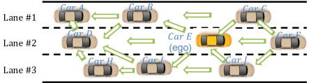
Figure 1: An illustrative scenario of a 3-lane freeway. It shows the vision sharing flow of all the vehicles. There could be human-driven vehicles on street. To make communication relations clear, we only show CAVs here.

Each vehicle sense its own onboard camera and LIDAR data. It is unrealistic to share the raw camera images and point clouds from LIDAR with others due to the following two reasons: (i) the limited bandwidth of a V2V link (Miller and Rim 2020); (ii) the same shared information on surrounding vehicles needs to be repeatedly learned for lane information extraction, resulting in computing resource waste. Hence, we first process the vision information locally using CNNs and then share the extracted features to other vehicles. Because the raw images and point clouds need to be synchronously processed and shared for behavior planning, we further develop a weight pruning technique to speed up the slower process.

CNN-Driven Shared Vision

We develop an end-to-end CNN-driven shared vision solution to derive the relative lane index of surrounding vehicles, i.e., which lane each surrounding vehicle is on. In Fig. 2, the shared vision model has two main branches. (i) Lane segmentation for global context and aggregates auxiliary segmentation task to utilize multi-scale features. The RGB images from the onboard camera are divided into equal-sized grids, and grids in the same rows are defined as row anchors. Grids with appearance of the lane mark on the row anchor will be colored green. Detailed pixel coordinates of all four-lane marks is generated by the network and saved in a hash table. (ii) The 3D OD (object detection) uses LIDAR point cloud as input. It converts raw point cloud to a sparse pseudo-image by stacking pillars and learning features from it for scatter (Qi et al. 2017). We process the pseudo-image into high-level representation by first continuously down-sampling learned features to small spatial resolution, then up-sampling and concatenating each down-sampled features, to predict 3D bounding boxes for neighbouring vehicles. The location of vehicles in camera coordinates, dimensions (height, width, length), observation angle, distance, and rotation is generated.

As camera RGB image and LIDAR point cloud are paired under same timestamp, in the second step, we derive the lane index of each surrounding vehicle by fusing the location and dimension of the surrounding vehicle (obtained by 3D OD) with coordinate of lane marks obtained by lane segmentation. We then send the lane index along with distance, observation angle, and rotation info to the DRL for behavior planning.

Weight Pruning to Enhance Synchronous Information Share

We observe that the processing time of point cloud data using PointPillars is significantly longer (11.16$\times$) than that of lane segmentation. The 3D OD becomes the “critical path” of the overall vision process. Therefore, we develop a weight pruning technique on the PointPillars network to reduce the running time. Many investigations have shown that there exists redundancy in CNN model parameters (Han et al. 2015; Iandola and Han 2016; Luo, Wu, and Lin 2017). CNN weight pruning can be used to exploit the redundancy in the parameterization of deep architectures, while maintaining the CNN model accuracy. We formulate the weight pruning problem in an $N$-layer CNN as: $\underset{\{{\bf{W}}_{i}\}}{\text{min}}~{}\mathcal{F}\big{(}\{{\bf{W}}_{i}\}_{i=1}^{N}\big{)},\text{subject to}~{}{\bf{W}}_{i}\in{\bf{S}}_{i},\;i=1,\ldots,N$, where ${\bf{W}}_{i}$ represents the weights in the $i$-th layer. $\mathcal{F}$ is the CNN loss function with respect to ${\bf{W}}_{i}$. ${\bf{S}}_{i}=\{{\bf{W}}_{i}\mid\mathrm{cardinality}({\bf{W}}_{i})\leq l_{i}\}$, where $l_{i}$ is desired numbers of non-zero weights. Through weight pruning, we bring acceleration in computation and reduction in memory, therefore satisfying the real-time requirement.

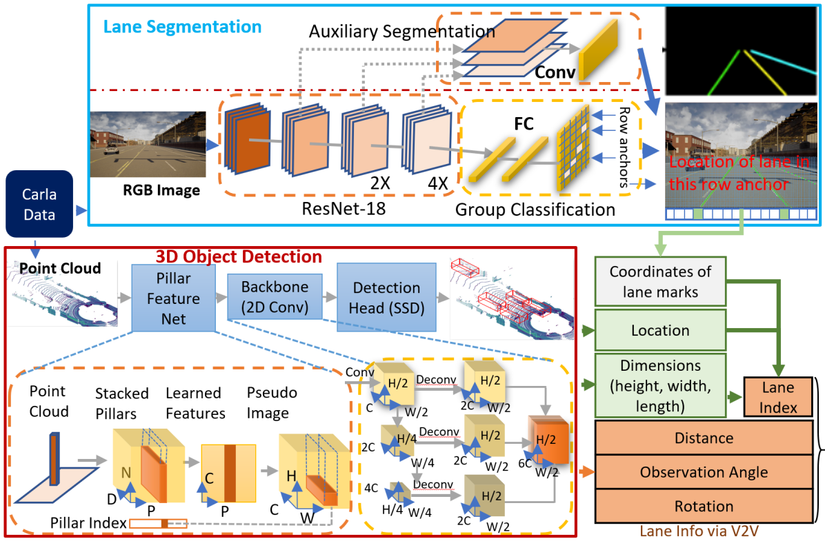
Figure 2: Detail structure of vision procedure

5 Behavior Planning

Since autonomous driving is a safety-critical application, the exploration policy in reinforcement learning (RL) for CAVs must be designed rigorously to avoid potential accidents. The action $a$ generated by the traditional $\epsilon$-greedy method (Mnih and Kavukcuoglu 2015) may not be safe. To ensure there are no collisions during the training process, we add a feedback process to find safe feasible actions.

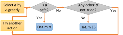
Figure 3: The safe action mapping $\Phi$ to get the safe action. If action $a$ is safe, then return the safe action $a$; if not, then try other actions; if no action is safe, then emergency stop (ES).

Safe Action Mapping

The safe action mapping $\Phi$ to get the safe action is shown in Fig. 3. Once the RL agent selects an action, we evaluates whether it is feasible to implement this action by checking safety constraints. If $a$ is safe, then the feedback action $a^{\prime}=a$; if not, we will search other actions in $\mathcal{A}$ that haven’t been tried and find a safe one. If all the actions in $\mathcal{A}$ are not safe in the worst case, then the controller will apply the emergency stop (ES) process. The ES is a special action that is not included in the action set $\mathcal{A}$. It will only be performed in an emergency scenario where all normal actions are not safe.

Safe Actor-Critic Algorithm

We design a safe actor-critic algorithm as shown in Alg. 1 for each CAV to learn a centralized critic $Q$ by minimizing the Bellman loss: $\mathcal{L}(\theta^{i})=\mathbb{E}_{o,a,r,o^{\prime}}[(y-Q^{i}(o,a;\theta^{i}))^{2}],$ where $y=r^{i}+\gamma\cdot Q^{\prime i}(o^{\prime},a^{\prime};\theta^{\prime i})|_{a^{\prime i}=\pi^{\prime i}(o^{\prime i})}$ and $Q^{\prime i}$ is the target network for the critic, $\pi^{\prime i}$ is the target network for the actor. Then we use this critic to train a localized actor $\pi^{i}(o^{i};\theta^{i})$ using the gradient $\nabla_{\theta^{i}}J=\mathbb{E}_{o,a\sim\mathcal{D}}\left[\nabla_{\theta^{i}}\pi^{i}(o^{i})\nabla_{a^{i}}Q^{i}(o,a)\right].$ In this algorithm, we use a replay buffer to store the transition experience $(o,a,r,o^{\prime})$, where $o$ is the current observation, $a$ is the action, $r$ is the reward, and $o^{\prime}$ is the next observation. The safe action mapping in Fig. 3 assures the policy used to produce a new transition experience is safe. When training the critic, a minibatch is sampled from the replay buffer to decorrelate data.

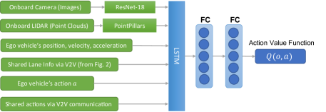
Figure 4: The $Q$-network for the behavior planning with the LSTM layer for the action-observation history. “FC” represents fully connected layer.

1 Randomly initialize the critic network $Q^{i}$ and the actor network $\pi^{i}$ for agent $i$. Initialize target networks $Q^{\prime i},\pi^{\prime i}$. Initialize the replay buffer $\mathcal{D}$;

2 for each episode do

3       Initialize the observation $o$;

4       for each timestep do

5             With probability $\epsilon$, select action $a^{i}=\Phi(\pi^{i}(o^{i}))$ for each agent $i$, where $\Phi$ is the safe action mapping in Fig. 3. With probability $1-\epsilon$, select an action $a^{i}$ for each agent $i$ in $\{\Phi(a^{i})|a^{i}\in\mathcal{A}\}$ randomly;

6            

7            Execute actions $a=(a^{1},...,a^{n})$ and observe reward $r$ and new observation $o^{\prime}$;

8            

9            Store $(o,a,r,o^{\prime})$ in replay buffer $\mathcal{D}$ and set $o\leftarrow o^{\prime}$;

10            

11            for each agent $i$ do

12                  

13                  Sample a random minibatch with size $K$ from $\mathcal{D}$;

14                  

15                  Set $y^{i}_{k}=r^{i}_{k}+\gamma Q^{\prime i}(o^{\prime}_{k},a^{\prime})|_{a^{\prime i}=\pi^{\prime i}(o^{\prime i})}$;

16                  

17                  Update critic by minimizing the loss $\mathcal{L}(\theta^{i})=\frac{1}{K}\sum_{k}(y_{k}^{i}-Q^{i}(o_{k},a_{k}))^{2}$;

18                  

19                  Update actor using the gradient $\nabla_{\theta^{i}}J=\frac{1}{K}\sum_{k}\nabla_{\theta^{i}}\pi^{i}(o^{i}_{k})\nabla_{a^{i}}Q^{i}(o_{k},a_{k})$ where $a^{i}=\pi^{i}(o^{i})$;

20                  

21                  Update target networks: $\theta^{\prime i}\leftarrow\tau\theta^{i}+(1-\tau)\theta^{\prime i}$.

22             end for

23            

24       end for

25      

26 end for

Algorithm 1 Safe Actor-Critic Algorithm

$Q$-network

The $Q$-network used in Alg. 1 is shown in Fig. 4. We consider the action set $\mathcal{A}$ includes {Keep Lane (KL), Change Left (CL), and Change Right (CR)}. The observation for each CAV includes: (i) onboard camera, LIDAR; (ii) position, velocity, and acceleration; (iii) processed shared vision information and actions of its immediate leaders on its current and neighbor lanes via V2V. Our algorithm also works in mixed traffic with both autonomous and human-driven vehicles. When there is no CAV in the surrounding vehicles, the ego vehicle can always use its onboard sensors’ information as the input of the $Q$-network.

Reward Function

We consider two system-level reward as evaluation criteria: average velocity $\bar{v}$ and average comfort $\bar{c}$. The comfort of single vehicle (for passenger’s experience) is defined based on its acceleration and action as follows:

$$c(\dot{v},a)=\begin{cases}3,&\text{if }\lvert\dot{v}\rvert<\Theta\text{ and }a=KL;\\ 2,&\text{if }\lvert\dot{v}\rvert\geq\Theta\text{ and }a=KL;\\ 1,&\text{if }a=CL/CR;\\ 0,&\text{if in }ES.\end{cases}$$ (1)

where $\dot{v}$ is the acceleration, $a\in\mathcal{A}$ is the behavior action, $\Theta$ is a predefined threshold. The reward function is defined as:

$$\mathbf{r}(s,a)=w\cdot\bar{v}+\bar{c},$$ (2)

where $s\in\mathcal{S}$, and $w$ is a trade-off weight.

6 Experiment

We use CARLA (Dosovitskiy and Ros 2017), an open source simulator which supports development, training, and validation of autonomous driving systems, to validate our proposed method. Each CAV is integrated with a camera sensor for capturing RGB images, and a LIDAR sensor for generating point clouds. The resolution of camera image is $375\times 1,242$ pixels. We set row anchors ranging from 100 to 370 with intervals of 10, and the number of grids is 100. We scale each image to $288\times 800$. Each point cloud from LIDAR is stored with the 3 coordinates (the ego vehicle being the origin), representing forward, left, and up respectively, and an additional reflectance value. To augment the dataset, we apply random mirroring flip along the forward axis, and a global rotation and scaling. In evaluation, we set forward and up axes’ resolution to $0.16m$, max number of pillars to 12,000, and max number of points per pillar to 100. Images and point clouds are paired under the same timestamp and are processed jointly under the CNN.

We assume all CAVs to share their processed vision information that includes features {lane index, distance, observation angle, rotation} of neighboring vehicles with their immediate followers as introduced in Section 4. Each CAV collects transition experience and store them in the replay buffer. Then they use minibatch gradient descent to learn the $Q$-function. The learning method detail is introduced in Section 5. The hyperparameters of our Alg. 1 is shown in Table 1.

Parameter	Value
optimizer	Adam
learning rate	0.01
discount factor	0.9
replay buffer size	$10^{6}$
hidden size in FC and LSTM layers	128
minibatch size	64
activation function	ReLU
frequency to update target network	100

Table 1: Safe Actor-Critic Hyperparameters.

The host machine adopted in our experiments is a server configured with Intel Core i9-10900X processors and four NVIDIA RTX2080Ti GPUs. Our experiments are performed on Python 3.7.6, GCC7 7.5, PyTorch 1.6.0, and CUDA 11.0.

CNN-Driven Shared Vision

For evaluation, PointPillars uses mean average precision (mAP) as standard, while Ultra-Fast-Lane-Detection uses “accuracy”, which is calculated as: $\frac{\sum_{\text{clip}}C_{\text{clip}}}{\sum_{\text{clip}}S_{\text{clip}}}$, where $C_{clip}$ is the number of lane points predicted correctly and $S_{clip}$ is the total number of ground truth in each clip. We show the performance (accuracy or mAP) and running speed in Table 2. The lane segmentation achieves high accuracy with low latency. It can process 313 images in one second. The 3D object detection has the running time of $28$ images per second (img/s), which means 100 images can be processed in around 3.6 seconds. Our weight pruning technique significantly increases the speed (by $3.5\times$) with a very small accuracy degradation. It decreases the processing time of 100 images from 3.6 seconds to one second. Overall, for the parallel lane segmentation and 3D object detection, our weight pruning technique significantly speeds up the CNN-driven shared vision process, satisfying real-time processing requirements. Our vision processing method can be used to mixed traffic setting that includes human-driven vehicles. The lane segmentation and object detection is the same when dealing with both autonomous and human-driven vehicles.

CNN Model	performance (%)	speed (img/s)
Lane	accuracy: 95.82	313
Segmentation
3D object	mAP: 76.5	28
detection (OD)
3D OD after	mAP: 73.6	99
weight pruning

Table 2: Summary of Result From Vision Network.

System Efficiency Improvement

In this section, we show our algorithm improves the CAVs’ system efficiency in terms of the average velocity and the average comfort as defined in the reward function (2).

Comparison Under Different CAV Ratios

Our approach improves the average velocity and the average comfort as the CAV ratios (the total CAV number divided by the total number of all vehicles) get higher. In this set of experiments, the total number of CAVs ranges from 0 to 30 as listed in Table 3. We compare the average velocity and comfort for all vehicles under different CAV ratios. The comfort of a single vehicle is defined in Eq. (1). It is averaged among all the vehicles as one criterion. The velocity and comfort are averaged over all the 40000 timesteps used in the simulation. The result of our approach is shown in Table 3. All CAVs use our safe actor-critic Alg. 1 introduced in Section 5. The result in Table 3 shows the average velocity and comfort of the entire mixed traffic. We use CARLA’s built-in human-driven vehicle in the mixed traffic (Dosovitskiy and Ros 2017). In the result of Table 3, the average velocity and comfort increase when the CAV ratio gets higher. This gives us insights that the penetration of the CAVs can improve traffic efficiency in the future.

CAV	CAV	HDV	average	average
ratio	number	number	velocity (mph)	comfort
0	0	30	60.06	2.61
0.17	5	25	61.82	2.64
0.33	10	20	64.70	2.68
0.5	15	15	65.14	2.72
0.67	20	10	65.18	2.74
0.83	25	5	65.53	2.77
1	30	0	66.15	2.81

Table 3: The system efficiency comparison under different CAV ratios. Our approach improves the average velocity and the average comfort as the CAV ratios get higher. (HDV: Human-driven vehicles)

Comparison Under Different Traffic Densities

Our approach improves the traffic flow and average comfort under different traffic densities. The traffic density $\rho$ is the ratio between the total number of vehicles and the road length. We compare the traffic flow and average comfort under different traffic densities among our safe MARL approach using Alg. 1, the MADDPG (Lowe and Wu 2017) algorithm and an intelligent driving model (IDM) (Talebpour and Mahmassani 2016). The traffic flow reflects the quality of the road throughout with respect to the traffic density. It is calculated as $\rho\times\bar{v},$ where $\bar{v}$ is the average velocity of all the vehicles (Rios-Torres and Malikopoulos 2018). The IDM is a common baseline in autonomous driving. In IDM, the vehicle’s acceleration is a function of its current speed, current and desired spacing, and the leading and following vehicles’ speed (Talebpour and Mahmassani 2016). Building on top of these IDM agents, we add lane-changing functionality using the gap acceptance method in (Butakov and Ioannou 2014). In this set of experiments, we keep CAV ratios at 0.6. As shown in Fig. 5, the safe MARL agent gets both larger traffic flow and better driving comfort when traffic density $\rho$ is low. When $\rho$ grows, the result of the safe MARL agent gets worse, but it is still comparable with the IDM. When the road is saturated, lane-changing tends to downgrade passengers’ comfort but cannot bring higher speed. Consequently, a better choice is to keep lanes when $\rho$ is high, and there is no significant difference between the safe MARL and the IDM. We also add the result using MADDPG in Fig. 5. Both the traffic flow and the driving comfort are very small (a positive number but close to 0) using MADDPG, and many collisions occurred during the simulation. This is because the MADDPG does not have a safety guarantee.

Figure 5: Our approach (safe MARL) improves the traffic flow and driving comfort under different traffic densities.

Safety Guarantee

In this section, we show our algorithm has a safety guarantee. We compare our safe actor-critic algorithm with the MADDPG (Lowe and Wu 2017) algorithm. We assign a negative reward in MADDPG for each collision. Our approach avoids the execution of unsafe actions that can lead to collisions. Table 4 shows the total number of unsafe actions executed by the safe MARL and MADDPG under different traffic densities. The traffic density $\rho$ is the ratio between the total number of vehicles and the road length. The number in Table 4 is averaged over the last 10 episodes, which has a maximum timestep of 40000. When $\rho=0.9$, our approach has 0 unsafe actions while the MADDPG has 242976 unsafe actions because it does not have a safety module.

$\rho$	0.1	0.2	0.3	0.4
Safe MARL	0	0	0	0
MADDPG	4416	9510	21897	43491
$\rho$	0.5	0.6	0.7	0.8
Safe MARL	0	0	0	0
MADDPG	61689	91154	133135	191404

Table 4: Total number of unsafe actions executed by the safe MARL and MADDPG under different traffic density $\rho$. Our approach has 0 unsafe action by using the safe action mapping.

Our approach can maintain a safe headway with neighboring vehicles while the MADDPG cannot. The headway is the distance between two consecutive vehicles following each other. In Fig. 6, the minimum headway across all the vehicles is shown in the first 500 timesteps of one episode when $\rho=0.6$. We see that the headway is always greater than 0 using our safe actor-critic algorithm with a minimum value of 18.5 meters. Nevertheless, the MADDPG is likely to have a negative headway, which means collisions in reality. Note that we set the minimum car-following distance of CAVs to be 18.5 meters following the study of the safe car-following distance of autonomous vehicles (Arechiga 2019), but this value can be set differently to satisfy the requirements in different scenarios.

Figure 6: Our approach (Safe MARL) can maintain a safe headway with neighboring vehicles while the MADDPG cannot. The figure shows the minimum headway across all the vehicles in the first 500 timesteps of one episode when $\rho=0.6$.

Our approach gets a much larger total episode reward than the MADDPG. The total episode reward is the summation of all stage-wise rewards defined in Eq. 2 for each episode. As shown on the left of Fig. 7, the maximum total episode reward using our approach is about 1940, which is firstly reached in the 20th episode. In the right figure, the maximum total episode reward using the MADDPG is about 7, because some collision terminates the episode. They have different initial rewards because the neural networks are randomly initialized and the action is selected by the $\epsilon$-greedy method with randomness. Our approach runs about 30 minutes in each episode as it has a safety guarantee and runs for the maximum episode length. Yet, each episode stops quickly in about 5 seconds using the MADDPG.

Figure 7: Our approach (safe MARL) gets a higher total episode reward compared to the MADDPG during the training process, because our approach can guarantee a safe training process and run for the maximum episode length.

Obstacle-At-Corner Scenario and Benefit of Shared Vision

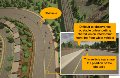
Figure 8: The obstacle-at-corner scenario where there are obstacles in a left-turning corner. The vehicles on the road are autonomous vehicles. The coming vehicles’ view is blocked such that they cannot observe the obstacles.

We construct a scenario called obstacle-at-corner to show how sharing vision information can help autonomous vehicles make wise lane-changing decisions ahead of time. As shown in Fig. 8, there are obstacles at a left-turning corner (represented by two stationary vehicles). The right bottom figure shows the view of a vehicle that comes in the direction of this curve road. It is quite difficult to observe the obstacles merely relying on its own sensors. In this case, if the white front vehicle can share its observation, the coming vehicle can get to know there are obstacles before entering the turning corner.

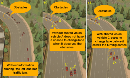
Figure 9: Without any information sharing, there is a traffic jam in the left lane. With shared vision from $A$ or $B$, using our safe MARL policy, vehicle $C$ can change its lane before it enters the left-turning corner.

Shared vision with our proposed safe MARL algorithm can help CAVs avoid traffic jams. We test our learned policy in the obstacle-at-corner scenario. When no vehicle can share information in subfigure (a) of Fig. 9, there are more vehicles blocked on the left-most lane and causing a traffic jam. Subfigures (b) and (c) are the screenshots taken in two close timesteps. In subfigure (b), vehicle $A$ is blocked in the left lane because there is vehicle $B$ in the middle lane and $A$ does not realize there are obstacles before it enters the corner (there is no neighboring vehicle that can share the obstacle information in advance in this scene; two obstacles are not CAVs). In subfigure (c), the coming vehicle $C$ in the left-most lane starts to change to the middle lane before it observes the obstacles because it gets the shared vision information either from $A$ or $B$. We use the safe action mapping introduced in Sec. 5 to ensure the safety of this lane-changing.

7 Conclusion

This paper studies how to solve behavior planning challenges for CAVs, that is, how to utilize V2V communication to improve traffic efficiency while also following safety requirements. We design an integrated information sharing and safe multi-agent reinforcement learning framework, which utilizes local observations and shared information in order to safely explore a behavior planning policy. The safe action mapping guarantees the safety of the training and execution process of the proposed MARL framework. We conduct the CAV simulation in CARLA. In the experiment, our weight pruning technique increases the speed of the 3D object detection (OD) by 3.5$\times$ with small accuracy degradation, since OD is the bottleneck for sharing vision. We also show that our approach improves the average velocity and average comfort under different CAV ratios and different traffic densities. Our approach avoids unsafe actions and maintains a safe distance from neighboring vehicles. We also construct the obstacle-at-corner scenario to show that the shared vision can help vehicles to avoid traffic jams. It is considered as future work to improve the robustness of the MARL policy under state uncertainties that are caused by V2V communication or sensor measurement errors.

References

- Alshiekh et al. (2018) Alshiekh, M.; Bloem, R.; Ehlers, R.; Könighofer, B.; Niekum, S.; and Topcu, U. 2018. Safe reinforcement learning via shielding. In AAAI, volume 32.
- Aradi (2022) Aradi, S. 2022. Survey of deep reinforcement learning for motion planning of autonomous vehicles. IEEE Trans. Intell. Transp. Syst., 23(2): 740–759.
- Arechiga (2019) Arechiga, N. 2019. Specifying safety of autonomous vehicles in signal temporal logic. In 2019 IEEE Intelligent Vehicles Symposium (IV), 58–63. IEEE.
- Bastani, Pu, and Solar-Lezama (2018) Bastani, O.; Pu, Y.; and Solar-Lezama, A. 2018. Verifiable reinforcement learning via policy extraction. In NeurIPS.
- Berkenkamp et al. (2017) Berkenkamp, F.; Turchetta, M.; Schoellig, A. P.; and Krause, A. 2017. Safe model-based reinforcement learning with stability guarantees. In NeurIPS.
- Buckman et al. (2020) Buckman, N.; Pierson, A.; Karaman, S.; and Rus, D. 2020. Generating Visibility-Aware Trajectories for Cooperative and Proactive Motion Planning. In ICRA 2020, 3220–3226. IEEE.
- Butakov and Ioannou (2014) Butakov, V. A.; and Ioannou, P. 2014. Personalized driver/vehicle lane change models for ADAS. IEEE Trans. Veh. Technol., 64(10): 4422–4431.
- Chen et al. (2015) Chen, C.; Seff, A.; Kornhauser, A.; and Xiao, J. 2015. Deepdriving: Learning affordance for direct perception in autonomous driving. In ICCV, 2722–2730.
- Chen, Li, and Tomizuka (2021) Chen, J.; Li, S. E.; and Tomizuka, M. 2021. Interpretable end-to-end urban autonomous driving with latent deep reinforcement learning. IEEE Trans. Intell. Transp. Syst.
- Chen et al. (2020) Chen, L.; Hu, X.; Tang, B.; and Cheng, Y. 2020. Conditional DQN-based motion planning with fuzzy logic for autonomous driving. IEEE Trans. Intell. Transp. Syst.
- Chen and Saulnier (2018) Chen, S.; and Saulnier, K. 2018. Approximating explicit model predictive control using constrained neural networks. In ACC, 1520–1527. IEEE.
- Cheng and Orosz (2019) Cheng, R.; and Orosz, G. 2019. End-to-end safe reinforcement learning through barrier functions for safety-critical continuous control tasks. In AAAI, volume 33, 3387–3395.
- Dosovitskiy and Ros (2017) Dosovitskiy, A.; and Ros, G. 2017. CARLA: An Open Urban Driving Simulator. In CoRL, 1–16.
- Fazlyab, Morari, and Pappas (2020) Fazlyab, M.; Morari, M.; and Pappas, G. J. 2020. Safety verification and robustness analysis of neural networks via quadratic constraints and semidefinite programming. IEEE Trans. Autom. Control.
- Fazlyab et al. (2019) Fazlyab, M.; Robey, A.; Hassani, H.; Morari, M.; and Pappas, G. J. 2019. Efficient and accurate estimation of lipschitz constants for deep neural networks. arXiv preprint arXiv:1906.04893.
- Fisac et al. (2019) Fisac, J. F.; Lugovoy, N. F.; Rubies-Royo, V.; Ghosh, S.; and Tomlin, C. J. 2019. Bridging hamilton-jacobi safety analysis and reinforcement learning. In ICRA, 8550–8556. IEEE.
- Foerster and Farquhar (2018) Foerster, J.; and Farquhar, G. 2018. Counterfactual multi-agent policy gradients. In AAAI.
- Han et al. (2015) Han, S.; Pool, J.; Tran, J.; and Dally, W. 2015. Learning both weights and connections for efficient neural network. In NeurIPS, 1135–1143.
- Hausknecht and Stone (2015) Hausknecht, M.; and Stone, P. 2015. Deep recurrent q-learning for partially observable mdps. arXiv:1507.06527.
- He et al. (2021) He, S.; Zeng, J.; Zhang, B.; and Sreenath, K. 2021. Rule-based safety-critical control design using control barrier functions with application to autonomous lane change. In ACC, 178–185. IEEE.
- Iandola and Han (2016) Iandola, F. N.; and Han, S. 2016. SqueezeNet: AlexNet-level accuracy with 50x fewer parameters and 0.5 MB model size. arXiv:1602.07360.
- Iqbal and Sha (2019) Iqbal, S.; and Sha, F. 2019. Actor-attention-critic for multi-agent reinforcement learning. In ICML, 2961–2970.
- Kenney (2011) Kenney, J. B. 2011. Dedicated Short-Range Communications (DSRC) Standards in the United States. Proceedings of the IEEE, 99(7): 1162–1182.
- Kim and Liu (2015) Kim, S.-W.; and Liu, W. 2015. The impact of cooperative perception on decision making and planning of autonomous vehicles. IEEE Intell. Transp. Syst. Mag., 7(3): 39–50.
- Le Mero et al. (2022) Le Mero, L.; Yi, D.; Dianati, M.; and Mouzakitis, A. 2022. A Survey on Imitation Learning Techniques for End-to-End Autonomous Vehicles. IEEE Trans. Intell. Transp. Syst.
- Lee and Park (2012) Lee, J.; and Park, B. 2012. Development and Evaluation of a Cooperative Vehicle Intersection Control Algorithm Under the Connected Vehicles Environment. IEEE Trans. Intell. Transp. Syst., 13(1): 81–90.
- Li and Bastani (2020) Li, S.; and Bastani, O. 2020. Robust model predictive shielding for safe reinforcement learning with stochastic dynamics. In ICRA, 7166–7172.
- Lowe and Wu (2017) Lowe, R.; and Wu, Y. I. 2017. Multi-agent actor-critic for mixed cooperative-competitive environments. In NeurIPS, 6379–6390.
- Lu et al. (2021) Lu, S.; Zhang, K.; Chen, T.; Başar, T.; and Horesh, L. 2021. Decentralized policy gradient descent ascent for safe multi-agent reinforcement learning. In AAAI, volume 35, 8767–8775.
- Luo, Wu, and Lin (2017) Luo, J.-H.; Wu, J.; and Lin, W. 2017. Thinet: A filter level pruning method for deep neural network compression. In ICCV, 5058–5066.
- Miller and Rim (2020) Miller, A.; and Rim, K. 2020. Cooperative Perception and Localization for Cooperative Driving. In ICRA 2020, 1256–1262. IEEE.
- Mnih and Kavukcuoglu (2015) Mnih, V.; and Kavukcuoglu, K. 2015. Human-level control through deep reinforcement learning. nature, 518(7540): 529–533.
- Oliehoek, Amato et al. (2016) Oliehoek, F. A.; Amato, C.; et al. 2016. A concise introduction to decentralized POMDPs, volume 1. Springer.
- Orosz and Ge (2017) Orosz, G.; and Ge, J. I. 2017. Seeing beyond the line of site–controlling connected automated vehicles. Mech Eng, 139(12): S8–S12.
- Ort, Paull, and Rus (2018) Ort, T.; Paull, L.; and Rus, D. 2018. Autonomous vehicle navigation in rural environments without detailed prior maps. In ICRA 2018, 2040–2047. IEEE.
- Pan et al. (2017) Pan, X.; You, Y.; Wang, Z.; and Lu, C. 2017. Virtual to real reinforcement learning for autonomous driving. In Proceedings of the British Machine Vision Conference (BMVC).
- Qi et al. (2017) Qi, C. R.; Su, H.; Mo, K.; and Guibas, L. J. 2017. Pointnet: Deep learning on point sets for 3d classification and segmentation. In CVPR, 652–660.
- Qin et al. (2021) Qin, Z.; Zhang, K.; Chen, Y.; Chen, J.; and Fan, C. 2021. Learning Safe Multi-Agent Control with Decentralized Neural Barrier Certificates. In ICLR.
- Rashid et al. (2020) Rashid, T.; Farquhar, G.; Peng, B.; and Whiteson, S. 2020. Weighted QMIX: Expanding Monotonic Value Function Factorisation for Deep Multi-Agent Reinforcement Learning. In NeurIPS.
- Rashid and Samvelyan (2018) Rashid, T.; and Samvelyan, M. 2018. QMIX: Monotonic Value Function Factorisation for Deep Multi-Agent Reinforcement Learning. In ICML, 4295–4304.
- Rios-Torres and Malikopoulos (2017) Rios-Torres, J.; and Malikopoulos, A. A. 2017. A Survey on the Coordination of Connected and Automated Vehicles at Intersections and Merging at Highway On-Ramps. IEEE Trans. Intell. Transp. Syst., 18(5): 1066–1077.
- Rios-Torres and Malikopoulos (2018) Rios-Torres, J.; and Malikopoulos, A. A. 2018. Impact of partial penetrations of connected and automated vehicles on fuel consumption and traffic flow. IEEE Trans. Intell. Veh, 3(4): 453–462.
- Shalev-Shwartz and Shammah (2016) Shalev-Shwartz, S.; and Shammah, S. 2016. Safe, multi-agent, reinforcement learning for autonomous driving. arXiv:1610.03295.
- Sunehag and Lever (2018) Sunehag, P.; and Lever, G. 2018. Value-Decomposition Networks For Cooperative Multi-Agent Learning Based On Team Reward. In AAMAS, 2085–2087.
- Talebpour and Mahmassani (2016) Talebpour, A.; and Mahmassani, H. S. 2016. Influence of connected and autonomous vehicles on traffic flow stability and throughput. Transp. Res. Part C Emerg. Technol., 71: 143–163.
- Thomas, Luo, and Ma (2021) Thomas, G.; Luo, Y.; and Ma, T. 2021. Safe reinforcement learning by imagining the near future. NeurIPS, 34: 13859–13869.
- Vinyals and Babuschkin (2019) Vinyals, O.; and Babuschkin, I. 2019. Grandmaster level in StarCraft II using multi-agent reinforcement learning. Nature, 575(7782): 350–354.
- Yu et al. (2019) Yu, C.; Wang, X.; Xu, X.; Zhang, M.; Ge, H.; Ren, J.; Sun, L.; Chen, B.; and Tan, G. 2019. Distributed multiagent coordinated learning for autonomous driving in highways based on dynamic coordination graphs. IEEE Trans. Intell. Transp. Syst., 21(2): 735–748.
- Zhang and Yang (2019) Zhang, K.; and Yang, Z. 2019. Multi-Agent Reinforcement Learning: A Selective Overview of Theories and Algorithms. arXiv:1911.10635.
- Zhang et al. (2016) Zhang, T.; Kahn, G.; Levine, S.; and Abbeel, P. 2016. Learning deep control policies for autonomous aerial vehicles with MPC-guided policy search. In ICRA, 528–535.
- Zhang et al. (2022) Zhang, T.; Song, W.; Fu, M.; Yang, Y.; Tian, X.; and Wang, M. 2022. A Unified Framework Integrating Decision Making and Trajectory Planning Based on Spatio-Temporal Voxels for Highway Autonomous Driving. IEEE Trans. Intell. Transp. Syst., 23(8): 10365–10379.
- Zhang, Bastani, and Kumar (2019) Zhang, W.; Bastani, O.; and Kumar, V. 2019. Mamps: Safe multi-agent reinforcement learning via model predictive shielding. arXiv:1910.12639.
- Zhou et al. (2020) Zhou, M.; Liu, Z.; Sui, P.; Li, Y.; and Chung, Y. Y. 2020. Learning Implicit Credit Assignment for Cooperative Multi-Agent Reinforcement Learning. In NeurIPS, volume 33, 11853–11864.