Uniform Preconditioners for High Order Finite Element Approximations of Planar Linear Elasticity

Abstract.

A new preconditioner is developed for high order finite element approximation of linear elastic problems on triangular meshes in two dimensions. The new preconditioner results in a condition number that is bounded independently of the degree $p$, the mesh-size $h$ and the ratio $\lambda/\mu$. The resulting condition number is reduced to roughly $6.0$ for all values of the parameters and discretization parameters on standard test problems. Crucially, the overall cost of the new preconditioner is comparable to the cost of applying standard domain decomposition based preconditioners.

1. Introduction

We consider conforming degree $p$ finite element discretization of the linear elasticity problem on meshes of triangular elements

(1.1) $$\bm{u}\in\bm{H}^{1}_{D}(\Omega):\qquad a_{\lambda}(\bm{u},\bm{v})=L(\bm{v})\qquad\forall\bm{v}\in\bm{H}^{1}_{D}(\Omega),$$

where $L(\cdot)$ is a continuous linear functional on $\bm{H}^{1}_{D}(\Omega)$ and

(1.2) $$a_{\lambda}(\bm{u},\bm{v}):=\int_{\Omega}\left\{2\mu\bm{\varepsilon}(\bm{u}):\bm{\varepsilon}(\bm{v})+\lambda(\operatorname{div}\bm{u})(\operatorname{div}\bm{v})\right\}\ d\bm{x}\qquad\forall\bm{u},\bm{v}\in\bm{H}^{1}(\Omega),$$

where $\bm{\varepsilon}(\cdot)$ is the strain tensor and $\bm{H}_{D}^{1}(\Omega)$ is the space of admissible displacements.

While the parameters $\mu$ and $\lambda$ need only be positive, the case where the ratio $\lambda/\mu\gg 1$ arises in several applications, e.g. nearly incompressible linear elasticity, where $\mu$ and $\lambda$ are the Lamé parameters, or in iterated penalty methods for incompressible flow [7, 18, 20], where $\nu=2\mu$ is the viscosity and $\lambda$ serves the role of an (artificial) penalty parameter associated with the incompressibility condition.

In each case, the fact that the ratio $\lambda/\mu\gg 1$ has various implications for the numerical approximation. Firstly, if the polynomial degree $p\in\{1,2,3\}$, then the finite element solution suffers from locking in the limit $\lambda/\mu\to\infty$ (see e.g. [12]). However, if the degree $p\geq 4$ then, under mild conditions on the mesh (see [8, Theorem 8.1]), both the $h$-version method with $p\geq 4$ and the pure $p$-version will be locking-free. For this reason, we will assume that $p\geq 4$ in what follows. Secondly, a more insidious problem is that the linear systems arising from discretizations of 1.1 become increasingly ill-conditioned as the ratio $\lambda/\mu$ increases, in addition to the usual ill-conditioning due to the mesh-size $h$ and the polynomial degree $p$. The objective of the current work is to develop a preconditioner which does not degenerate in any of the limits $p\to\infty$, $h\to 0$, or $\lambda/\mu\to\infty$.

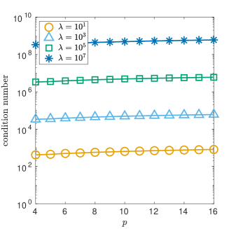
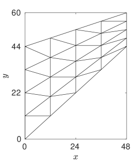
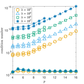
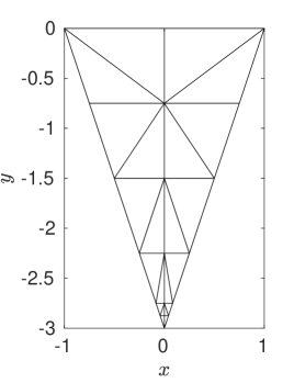
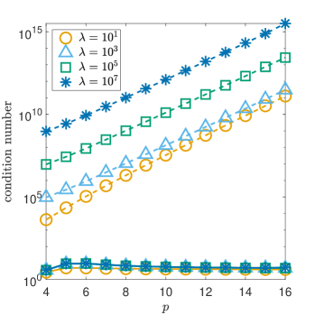
In order to illustrate both the seriousness of the problem and the fact that standard remedies fall short, we consider a simple example. The geometry for the Cook’s membrane problem and the domain are displayed in Figure 1(d) where the left hand face is held fixed and a vertical shear is applied on the right hand face. The problem is approximated using elements of degree $p$ in the range $\{4,\ldots,16\}$ on the fixed mesh shown in Figure 1(d) with material parameters $\mu=1$ and $\lambda\in\{10^{1},10^{3},10^{5},10^{7}\}$.

(a)

(b)

(c)

(d)

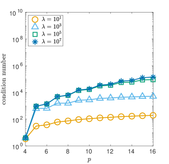
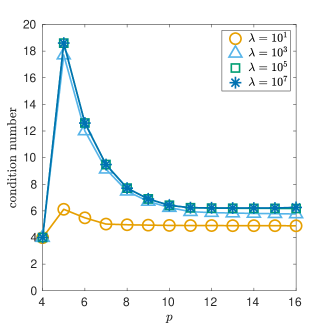
Figure 1. (a-b) Condition numbers using the preconditioner in [11] with (a) $p=1$ coarse space and (b) $p=4$ coarse space, (c) condition numbers using the preconditioner in section 3.2, and (d) computational mesh. Observe that the condition numbers in (b) are bounded as $\lambda$ grows, but grow more rapidly than those in (a) as a function of $p$, while the condition numbers in (c) are uniformly bounded in $p$ and $\lambda$.

Figure 1(a) shows the condition number obtained when the standard preconditioner developed by Babuška et al. [11] is used, which is known to reduce the growth of the condition number to $\mathcal{O}(1+\log^{2}p)$ and to be independent of the mesh size $h$. While the results shown in Figure 1(a) are consistent with this fact, one observes that the actual condition number is proportional to the ratio $\lambda/\mu$ which means that even though the effects of $h$ and $p$ are controlled, the hidden constant in the $\mathcal{O}(1+\log^{2}p)$ estimate degenerates as $\lambda/\mu\to\infty$.

The preconditioner of Babuška et al. is based on domain decomposition in conjunction with a coarse grid solver using a piecewise linear finite element subspace on the mesh. Interestingly, enlarging the coarse space to consist of piecewise quartic functions results in a preconditioner that does not degenerate at all as the ratio $\lambda/\mu$ increases as shown in Figure 1(b). Unfortunately, the results indicate that the condition number now grows rapidly with the polynomial degree $p$, even though the only change compared with the standard Babuška et al. preconditioner was to enlarge the coarse space.

The current work provides an explanation for these observations but, more importantly, a new preconditioner is developed that gives rise to a condition number that is bounded independently of the degree $p$, the mesh-size $h$ and the ratio $\lambda/\mu$. The performance of the new preconditioner on the Cook’s membrane problem is illustrated in Figure 1(c) where it is seen that the condition number is reduced to roughly $6.0$ for all values of the parameters and discretization parameters. Crucially, the overall cost of the new preconditioner is comparable to the cost of applying standard domain decomposition based preconditioners such as the Babuška et al. scheme.

While various preconditioners for conforming finite element approximations of 1.1 have already received some attention in the literature, e.g. [25, 37], these works do not attempt to quantify or control the dependence on the polynomial degree $p$. Here, we fully account for the $p$ dependence and show that the resulting condition number is independent of $p$ as well as the mesh size $h$.

In section 3, we describe a family of Additive Schwarz preconditioners that control the condition number of the preconditioned system not just with respect to $\mu$, $\lambda$, and $h$, but also with respect to the polynomial degree $p$. The subspace decomposition consists of a coarse space containing the lowest order $(p=4)$ elements and, for each vertex, a local solve associated with the functions supported on the patch of elements abutting the vertex. The use of a low order coarse space is standard for high order preconditioners [1, 2, 6, 11, 22, 30, 31, 32, 33], while the vertex patch spaces, although more common in $H(\mathrm{div})$ and $H(\mathrm{curl})$ applications (see e.g. [9, 10, 23, 24]), have also previously appeared in the $H^{1}$ context [25, 30, 33, 37]. Using technical results established in [25, 26, 37], we show that the condition number of the preconditioned system is uniform in $\mu$, $\lambda$, $h$, and $p$ for suitable choices of the space of functions associated with element boundaries. Several of these choices are detailed and the effectiveness of the preconditioner is showcased in several numerical examples in section 4, while the remainder of the paper is devoted to the analysis.

2. Problem Setup

Let $X\subset H^{1}(\Omega)$ be the space of continuous, piecewise polynomials of degree $p\in\mathbb{N}$ on a triangulation $\mathcal{T}$ of $\Omega$:

(2.1) $$X:=\{v\in C(\bar{\Omega}):v|_{K}\in\mathcal{P}_{p}(K)\ \forall K\in\mathcal{T}\},$$

where $\mathcal{P}_{p}(K)$ denotes the space of polynomials of degree at most $p$. In particular, we assume that the triangulation $\mathcal{T}$ is a shape-regular partitioning of the domain $\Omega$ into triangles such that the nonempty intersection of any two distinct elements from $\mathcal{T}$ is either a single common vertex or a single common edge of both elements with mesh size $h:=\max_{K\in\mathcal{T}}h_{K}$ and $h_{K}:=\mathrm{diam}(K)$. We also assume that mesh vertices are placed at the intersections of $\bar{\Gamma}_{D}$ and $\bar{\Gamma}_{N}$. The subspace $X_{D}:=X\cap H^{1}_{D}(\Omega)$ then consists of functions in $X$ vanishing on the Dirichlet boundary $\Gamma_{D}$.

We discretize 1.1 using the space $\bm{X}_{D}:=X_{D}\times X_{D}$ as follows:

(2.2) $$\bm{u}_{X}\in\bm{X}_{D}:\qquad a_{\lambda}(\bm{u}_{X},\bm{v})=L(\bm{v})\qquad\forall\bm{v}\in\bm{X}_{D}.$$

By fixing a basis for $\bm{X}_{D}$, we may express 2.2 as a linear system of equations:

(2.3) $$\bm{A}\vec{u}=\vec{L},$$

where $\bm{A}$ is the stiffness matrix, $\vec{L}$ is the load vector, and $\vec{u}$ is the vector of degrees of freedom of $\bm{u}$. As mentioned in section 1 and shown in the numerical examples in section 4, the conditioning of the matrix $\bm{A}$ generally degenerates rapidly as $\mu\to 0$, as $\lambda\to\infty$, as $h\to 0$, and/or as $p\to\infty$. In order to help solve the matrix equation 2.3 efficiently, we seek ASM preconditioners for $\bm{A}$ which remove the growth of the condition number in these parameters.

3. Additive Schwarz Preconditioners

Let

(3.1) $$\bm{X}_{I}:=\bigoplus_{K\in\mathcal{T}}\bm{X}_{I}(K),\qquad\text{where}\quad\bm{X}_{I}(K):=\{\bm{v}\in\bm{X}_{D}:\operatorname{supp}\bm{v}\subseteq K\}$$

be the space of interior functions, i.e. functions vanishing on element boundaries, and let $\bm{X}_{B}\subset\bm{X}$ be any subspace such that the following (direct sum) identity holds:

(3.2) $$\bm{X}_{D}=\bm{X}_{I}\oplus\bm{X}_{B}.$$

Each $\bm{v}_{I}\in\bm{X}_{I}$ vanishes on the element boundaries, i.e. $\bm{v}_{I}|_{\partial K}=\bm{0}$ for all $K\in\mathcal{T}$, and so the space $\bm{X}_{B}$ corresponds to the degrees of freedom associated with element boundaries. 3.2 means that for each $\bm{v}\in\bm{X}_{D}$, there exist unique $\bm{v}_{I}\in\bm{X}_{I}$ and $\bm{v}_{B}\in\bm{X}_{B}$ such that $\bm{v}=\bm{v}_{I}+\bm{v}_{B}$. Specifically, the uniqueness of $\bm{v}_{B}$ means that one can define a mapping $\mathbb{T}_{B}:\bm{X}_{D}\to\bm{X}_{B}$ by the rule $\mathbb{T}_{B}\bm{v}=\bm{v}_{B}$. However, it is important to distinguish this uniqueness from the fact that the choice of $\bm{X}_{B}$ itself is far from unique owing to the considerable freedom in choosing the form of the functions in $\bm{X}_{B}$ on the element interiors. Moreover, the effectiveness of the ASM based on the decomposition 3.2 will depend heavily on the choice of $\bm{X}_{B}$. We shall discuss this further along with some suitable choices in section 4.

3.1. Decomposition of Boundary Space

As mentioned above, the space $\bm{X}_{B}$ corresponds to the degrees of freedom associated with element vertices $\mathcal{V}$ and edges $\mathcal{E}$. In the interests of efficiency, it is useful to further decompose the boundary space $\bm{X}_{B}$ into (overlapping) subspaces $\bm{X}_{C}$ and $\{\bm{X}_{\bm{a}}:\bm{a}\in\mathcal{V}\}$ as follows: The coarse space consists of the lowest order (in this case $p=4$) elements on the element boundaries:

(3.3) $$\bm{X}_{C} :=\{\bm{v}\in\bm{X}_{B}:\bm{v}|_{\gamma}\in\bm{\mathcal{P}}_{4}(\gamma)\ \forall\gamma\in\mathcal{E}\}.$$

Although $\bm{X}_{C}$ consists of piecewise polynomials whose restrictions to element edges are polynomials of degree at most 4, the fact that $\bm{X}_{C}\subseteq\bm{X}_{B}$ means their values on the element interiors will be polynomials of degree $p$. The subspace $\bm{X}_{\bm{a}}$ associated with a vertex $\bm{a}\in\mathcal{V}$ consists of functions supported on the patch $\mathcal{T}_{\bm{a}}$ comprising of elements which abut $\bm{a}$:

(3.4) $$\bm{X}_{\bm{a}}:=\{\bm{v}\in\bm{X}_{B}:\operatorname{supp}\bm{v}\subseteq\mathcal{T}_{\bm{a}}\},\ \bm{a}\in\mathcal{V}.$$

The space $\bm{X}_{B}$ then admits the following (overlapping) decomposition:

(3.5) $$\bm{X}_{B}=\bm{X}_{C}+\sum_{\bm{a}\in\mathcal{V}}\bm{X}_{\bm{a}}.$$

3.2. Preconditioners

Algorithm 1 Action of ASM Preconditioner $P^{-1}$ on residual $r\in\bm{X}_{D}^{*}$

(3.6a) $$\bm{u}_{I,K}\in\bm{X}_{I}(K) :\qquad a_{\lambda,K}(\bm{u}_{I,K},\bm{v}) =r(\bm{v})\qquad \forall\bm{v}\in\bm{X}_{I}(K),\ \forall K\in\mathcal{T},$$

(3.6b) $$\bm{u}_{C}\in\bm{X}_{C} :\qquad a_{\lambda}(\bm{u}_{C},\bm{v}) =r(\bm{v})\qquad \forall\bm{v}\in\bm{X}_{C},$$

(3.6c) $$\bm{u}_{\bm{a}}\in\bm{X}_{\bm{a}} :\qquad a_{\lambda}(\bm{u}_{\bm{a}},\bm{v}) =r(\bm{v})\qquad \forall\bm{v}\in\bm{X}_{\bm{a}},\ \forall\bm{a}\in\mathcal{V}.$$

$P^{-1}r:=\sum_{K\in\mathcal{T}}\bm{u}_{I,K}+\bm{u}_{C}+\sum_{\bm{a}\in\mathcal{V}}\bm{u}_{\bm{a}}$.

The subspace decomposition 3.2 along with the further decomposition 3.5 gives rise to an ASM preconditioner $P^{-1}:\bm{X}_{D}^{*}\to\bm{X}_{D}$ whose action on a residual $r\in\bm{X}_{D}^{*}$ is defined in Algorithm 1. The sequence of interior corrections in 3.6a is equivalent to a single interior correction

$$\bm{u}_{I}\in\bm{X}_{I}:\qquad a_{\lambda}(\bm{u}_{I},\bm{v})=r(\bm{v})\qquad\forall\bm{v}\in\bm{X}_{I}$$

thanks to 3.1 and the identity $a_{\lambda}(\bm{u},\bm{v})=\sum_{K\in\mathcal{T}}a_{\lambda,K}(\bm{u},\bm{v})$, where $a_{\lambda,K}(\cdot,\cdot)$ denotes the restriction of $a_{\lambda}(\cdot,\cdot)$ to an element $K$.

We shall quantify the effectiveness of the preconditioner $P^{-1}$ in terms of two parameters $\beta_{X}$ and $\tau_{B}$. The first of these parameters is the inf-sup constant $\beta_{X}$ for the pair $\bm{X}_{D}\times\operatorname{div}\bm{X}_{D}$:

(3.7) $$\beta_{X}:=\inf_{0\neq q\in\operatorname{div}\bm{X}_{D}}\sup_{\bm{0}\neq\bm{v}\in\bm{X}_{D}}\frac{(q,\operatorname{div}\bm{v})}{\|q\|\ \|\bm{v}\|_{1}},$$

where $(\cdot,\cdot)$ denotes the $L^{2}(\Omega)$ or $\bm{L}^{2}(\Omega)$ inner product and $\|\cdot\|_{s}$ denotes the $H^{s}(\Omega)$ or $\bm{H}^{s}(\Omega)$ norm. For elements of degree $p\geq 4$, it is known [8, Theorem 5.1] that $\beta_{X}$ is bounded below by a positive constant, $\beta_{0}$ independent of $h$ and $p,$ under certain (mild) assumptions on the mesh $\mathcal{T}$; see e.g. [8, p. 35] for a detailed characterization of the conditions. The inf-sup constant $\beta_{X}$ is more commonly associated with the mixed FEM discretization of the Stokes problem. However, its appearance in the current setting is to be expected since the linear elasticity problem (formally) converges to the Stokes flow in the incompressible limit $\lambda\to\infty$ with which we are concerned.

The second parameter $\tau_{B}$ quantifies the effect of the freedom in the choice of boundary space $\bm{X}_{B}$ alluded to at the start of this section. Often, the first step in preconditioning high order elements is to statically condense or eliminate the interior degrees of freedom [1, 2, 6, 11, 22, 31, 32, 33]. Static condensation corresponds to defining the values of a function $\bm{v}\in\bm{X}_{B}$ on the interior of an element $K\in\mathcal{T}$ to be the minimum energy extension of the values of $\bm{v}|_{\partial K}$. More precisely, if we define an operator $\mathbb{H}:\bm{X}_{D}\to\bm{X}_{D}$ by the rule

(3.8a) $$a_{\lambda}(\mathbb{H}\bm{u},\bm{v}) =0\qquad \forall\bm{v}\in\bm{X}_{I},$$

(3.8b) $$(\mathbb{H}\bm{u}-\bm{u})|_{\partial K} =\bm{0}\qquad \forall K\in\mathcal{T},$$

then the boundary space $\bm{X}_{B}$ corresponding to static condensation may be written equally well in any of the following ways:

(3.9) $$\bm{X}_{B}=\mathbb{H}\bm{X}_{D}=\bm{X}_{D}\cap\bm{X}_{I}^{\perp}=\{\bm{v}\in\bm{X}_{D}:a_{\lambda}(\bm{v},\bm{w})=0\ \forall\bm{w}\in\bm{X}_{I}\}.$$

In this case, the decomposition $\bm{v}=\bm{v}_{I}+\bm{v}_{B}=\bm{v}_{I}+\mathbb{H}\bm{v}$ is orthogonal (so that in this case $\mathbb{T}_{B}=\mathbb{H}$) and satisfies the following estimate for all $\bm{v}\in\bm{X}_{D}$:

$$\|\bm{\varepsilon}(\mathbb{T}_{B}\bm{v})\|^{2}+\frac{\lambda}{2\mu}\|\operatorname{div}\mathbb{T}_{B}\bm{v}\|^{2}=\frac{1}{2\mu}a_{\lambda}(\mathbb{T}_{B}\bm{v},\mathbb{T}_{B}\bm{v}) \leq\frac{1}{2\mu}a_{\lambda}(\bm{v},\bm{v})$$

(3.10) $$\leq\left(1+\frac{\lambda}{\mu}\right)\|\bm{\varepsilon}(\bm{v})\|^{2},$$

where the final inequality uses $\|\operatorname{div}\bm{v}\|^{2}\leq 2\|\bm{\varepsilon}(\bm{v})\|^{2}$. Choosing $\bm{X}_{B}$ to comprise of minimum energy extensions is natural and, in many cases, largely effective in controlling the growth of the condition number [1, 2, 6, 11, 22, 31, 32, 33]. However, in the present setting, as we shall see, if the analysis of the preconditioner is based on 3.10, then the presence of $\lambda/\mu$ in the multiplier on the RHS gives rise to a bound on the condition number which degenerates as $\lambda/\mu\to\infty$.

In order to obtain estimates for the performance of the preconditioner that are robust with respect to the ratio $\lambda/\mu$, one would like to choose $\bm{X}_{B}$ so that the corresponding operator $\mathbb{T}_{B}$ satisfies an estimate of the form 3.10 in which the multiplier appearing on the RHS is independent of $\lambda/\mu$. In general, this is not possible owing to the presence of the term $(\lambda/\mu)\|\operatorname{div}\mathbb{T}_{B}\bm{v}\|^{2}$ which blows up as $\lambda/\mu\to\infty$.

Instead, we relax the condition 3.10 by replacing the term $(\lambda/\mu)\|\operatorname{div}\mathbb{T}_{B}\bm{v}\|^{2}$ with a smaller quantity as follows; the parameter $\tau_{B}$ is defined to be any constant such that the following condition holds:

(3.11) $$\|\bm{\varepsilon}(\mathbb{T}_{B}\bm{v})\|^{2}+\lambda\mu^{-1}\|\Pi_{I}\operatorname{div}\mathbb{T}_{B}\bm{v}\|^{2}\leq\tau_{B}^{2}\|\bm{\varepsilon}(\bm{v})\|^{2}\qquad\forall\bm{v}\in\bm{X}_{D},$$

where $\Pi_{I}:L^{2}(\Omega)\to\operatorname{div}\bm{X}_{I}$ denotes the $L^{2}(\Omega)$ projection operator onto $\operatorname{div}\bm{X}_{I}$: i.e.

$$(\Pi_{I}q,r)=(q,r)\qquad\forall r\in\operatorname{div}\bm{X}_{I},\forall q\in L^{2}(\Omega).$$

The key difference between 3.10 and 3.11 is that the full divergence $\operatorname{div}\mathbb{T}_{B}\bm{v}$ has been replaced with its projection onto the interior divergence space $\Pi_{I}\operatorname{div}\mathbb{T}_{B}\bm{v}$. The presence of the projection operator $\Pi_{I}$ in the term $\|\Pi_{I}\operatorname{div}\mathbb{T}_{B}\bm{v}\|$ is reminiscent of reduced integration operators that play an important role in finite element methods for nearly incompressible linear elasticity; see e.g. [14, §8.12].

Our main result quantifies the performance of $P^{-1}$ in terms of the factors $\beta_{X}$ and $\tau_{B}$ defined in 3.7 and 3.11:

Theorem 3.1.

Let $\bm{P}^{-1}$ denote the matrix form of $P^{-1}$ and suppose that 3.7 and 3.11 hold. Then,

(3.12) $$\operatorname{cond}(\bm{P}^{-1}\bm{A})\leq C(1+\beta_{X}^{-2})(1+\tau_{B}^{2}),$$

where $C$ is independent of $\beta_{X}$, $\tau_{B}$, $\mu$, $\lambda$, $h$, and $p$.

4. Three Choices of Boundary Space

In this section, we present three options for choosing the space $\bm{X}_{B}$, all of which offer computational benefits in various setting, and will be shown to satisfy 3.11 with $\tau_{B}$ independent of $\lambda/\mu$.

4.1. Static Condensation

We start by returning to the choice 3.9 where $\bm{X}_{B}$ is defined in term of static condensation. As already pointed out, the multiplier on the RHS in 3.10 degenerates as $\lambda/\mu\to\infty$. However, as we shall show in Theorem C.1, the weakened form 3.11 does hold with $\tau_{B}$ independent of $\mu$, $\lambda$, $h$, and $p$. Theorem 3.1 then gives the bound

(4.1) $$\operatorname{cond}(\bm{P}^{-1}\bm{A})\leq C(1+\beta_{X}^{-2}),$$

where $C$ is independent of $\beta_{X}$, $\mu$, $\lambda$, $h$, and $p$.

In practice, static condensation allows one to compute the solution to 2.2 more efficiently than suggested in Algorithm 1. The orthogonality condition in 3.9 means that the stiffness matrix $\bm{A}$ and preconditioner $\bm{P}$ take the form

$$\bm{A}=\begin{bmatrix}\bm{A}_{II}&\bm{0}\\ \bm{0}&\bm{A}_{BB}\end{bmatrix}\quad\text{and}\quad\bm{P}^{-1}=\begin{bmatrix}\bm{A}_{II}^{-1}&\bm{0}\\ \bm{0}&\bm{P}_{BB}^{-1}\end{bmatrix},$$

where $\bm{A}_{II}$ corresponds to the interactions between the interior degrees of freedom and $\bm{A}_{BB}$ and $\bm{P}_{BB}^{-1}$ correspond to the element boundary interactions. We partition the solution and load vectors analogously. As a result, the interior and boundary components of the solution $\bm{u}$ are decoupled:

(4.2) $$\vec{u}=\begin{bmatrix}\vec{u}_{I}\\ \vec{u}_{B}\end{bmatrix},\qquad\text{where}\quad\bm{A}_{II}\vec{u}_{I}=\vec{L}_{I}\quad\text{and}\quad\bm{A}_{BB}\vec{u}_{B}=\vec{L}_{B}.$$

We choose to invert $\bm{A}_{II}$ element-by-element as indicated in 3.6a using a direct method, while we use the conjugate gradient method with preconditioner $\bm{P}_{BB}^{-1}$ to compute $\vec{u}_{B}$. The key point is that the interior degrees of freedom are computed only once, and not every iteration of the iterative solver. In addition, the performance of $\bm{P}_{BB}^{-1}$ is identical to the performance of $\bm{P}^{-1}$ since in this case $\operatorname{cond}(\bm{P}_{BB}^{-1}\bm{A}_{BB})=\operatorname{cond}(\bm{P}^{-1}\bm{A})$.

Cook’s Membrane. We now demonstrate the performance of the preconditioner $\bm{P}$ on the Cook’s membrane problem mentioned in section 1. More precisely, the boundary conditions are

$$\bm{u} =\bm{0},\qquad \text{on }\{0\}\times(0,44),$$

$$\bm{\sigma}(\bm{u})\bm{n} =(1,0)^{T},\qquad \text{on }\{48\}\times(44,60),$$

$$\bm{\sigma}(\bm{u})\bm{n} =\bm{0}\qquad \text{on the remainder of $\Gamma$},$$

where $\bm{\sigma}(\bm{u})_{ij}:=2\mu\bm{\varepsilon}(\bm{u})_{ij}+\lambda(\operatorname{div}\bm{u})\delta_{ij}$ is the stress tensor. The condition numbers of the full stiffness matrix $\bm{A}$, the boundary component $\bm{A}_{BB}$, and the preconditioned boundary system $\bm{P}_{BB}^{-1}\bm{A}_{BB}$ with $\mu=1$ and $\lambda\in\{10^{1},10^{3},10^{5},10^{7}\}$ are shown in Figure 2(a). Consistent with 4.1, the condition numbers of $\bm{P}_{BB}^{-1}\bm{A}_{BB}$ are uniformly bounded in $\lambda$ and $p$, and the preconditioned conjugate gradient method converges in a constant number of iterations, independently of $p$ and $\lambda$.

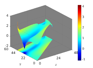
The benefit of using high polynomial degree is demonstrated in Figure 2(b), which displays the log of the von Mises stress for the $p=16$ solution with $\lambda=10^{5}$. The von Mises stress [36], a failure criterion for a material, is given by $\sigma_{v}^{2}:=\sigma_{11}^{2}+\sigma_{22}^{2}+3\sigma_{12}^{2}-\sigma_{11}\sigma_{22}$, and in particular depends on the gradient of the solution. With a coarse mesh, the $p=16$ solution is able to capture both the singularity at $(0,44)$ and the smooth profile of $\sigma_{v}$ away from the singularity.

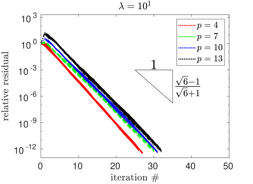
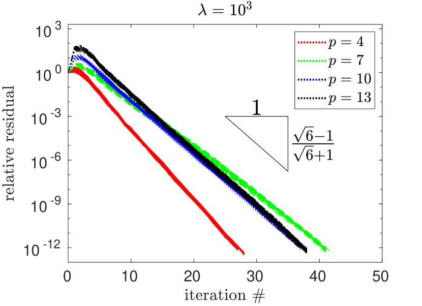
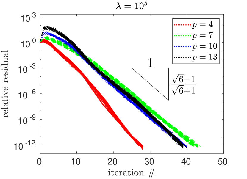
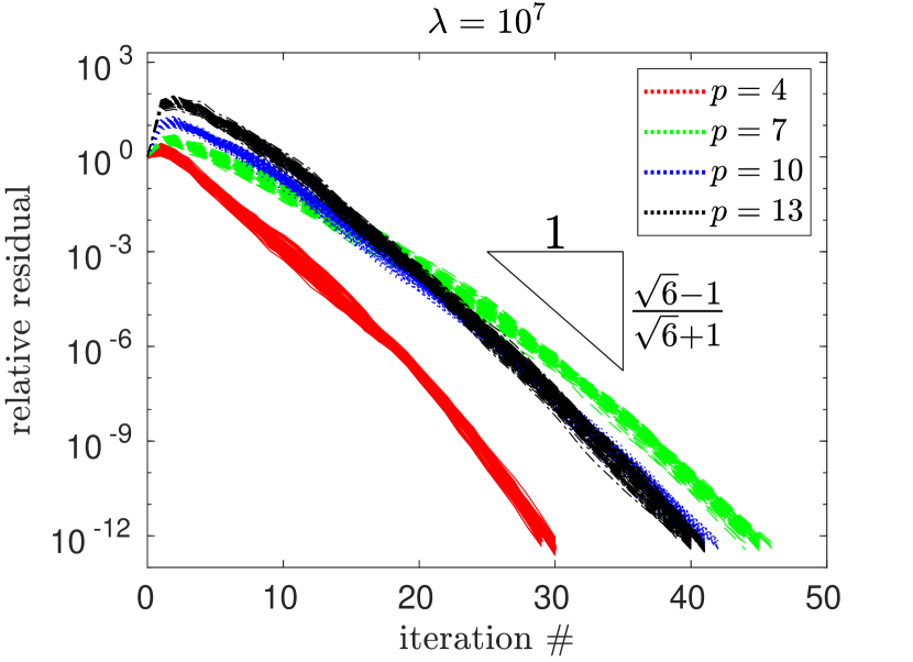
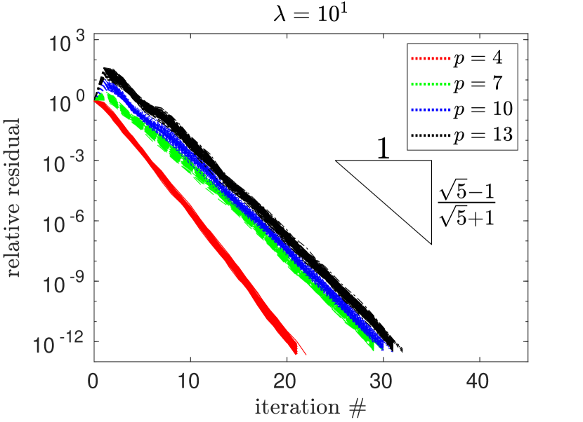
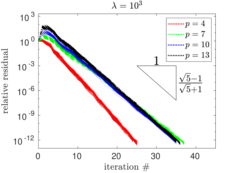
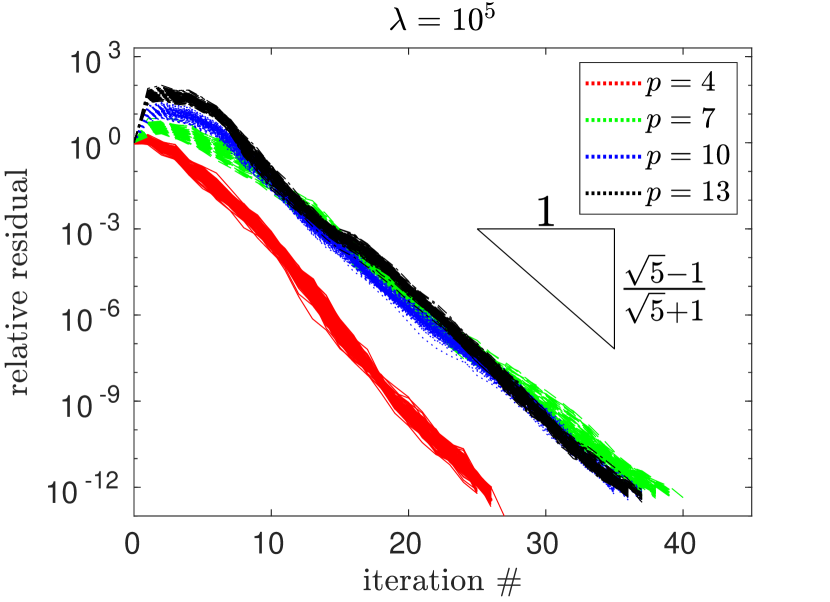
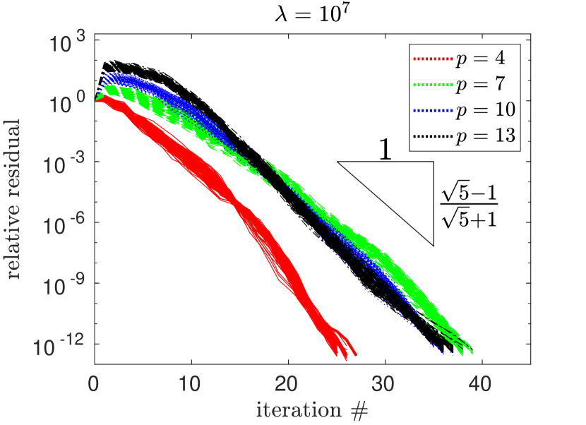
The residual history for $p\in\{4,7,10,13\}$ for the same choices of $\mu$ and $\lambda$ as above are displayed in Figure 3. In order to avoid biasing the results by the choice of data, we show an ensemble of curves for each value of $p$ corresponding to 100 random choices of the vector $\vec{b}$ with entries uniformly distributed in $(-1,1)$ and zero starting vector. Here, and in the remaining examples, the relative residual is defined to be $\|\vec{r}_{k}\|_{\ell^{2}}/\|\vec{r}_{0}\|_{\ell^{2}}$, where $r_{k}:=\bm{A}_{BB}\vec{x}_{k}-\vec{b}$ is the residual vector at the $k$-th step, and iteration is terminated when the relative residual is smaller than $10^{-12}$. Consistent with the theory (see e.g. [21, p. 636]), conjugate gradient converges in a constant number of iterations that is insensitive to the value of $p$ or $\lambda$, and the relative residual decreases at the geometric rate $(\sqrt{\kappa}-1)/(\sqrt{\kappa}+1)$, where $\kappa=\operatorname{cond}(\bm{P}_{BB}^{-1}\bm{A}_{BB})\simeq 6.0$.

(a)

(b)

Figure 2. Cook’s membrane problem (a) condition numbers of $\bm{A}$ (dotted lines), $\bm{A}_{BB}$ (dashed lines), and $\bm{P}_{BB}^{-1}\bm{A}_{BB}$ (solid lines) and (b) log of the von Mises stress for the $p=16$ solution with $\lambda=10^{5}$. Observe that the condition numbers of $\bm{P}_{BB}^{-1}\bm{A}_{BB}$ level out around 6.

(a)

(b)

(c)

(d)

Figure 3. Residual history of the conjugate gradient method with preconditioner $\bm{P}$ applied to the Cook’s membrane problem with (a) $\lambda=10^{1}$, (b) $\lambda=10^{3}$, (c) $\lambda=10^{5}$, and (d) $\lambda=10^{7}$.

4.2. The SCIP Method

For certain applications [7], it is advantageous to choose the boundary space as follows:

(4.3) $$\tilde{\bm{X}}_{B}:=\{\bm{v}\in\bm{X}_{D}:a_{\lambda}(\bm{v},\bm{z})=0\ \forall\bm{z}\in\bm{X}_{I}:\operatorname{div}\bm{z}\equiv 0\\ \text{and}\quad(\operatorname{div}\bm{v},\operatorname{div}\bm{w})=0\ \forall\bm{w}\in\bm{X}_{I}\}.$$

As shown in Lemma 5.4, the space $\tilde{\bm{X}}_{B}$ satisfies condition 3.11 with $\tau_{B}$ independent of $\mu$, $\lambda$, $h$, and $p$ so that Theorem 3.1 again shows that the associated preconditioner remains effective:

(4.4) $$\operatorname{cond}(\bm{P}^{-1}\bm{A})\leq C(1+\beta_{X}^{-2}).$$

The space $\tilde{\bm{X}}_{B}$ naturally arises in finite element analysis of incompressible flow. For example, as discussed in [7], the pair $\bm{X}_{D}\times\operatorname{div}\bm{X}_{D}$, i.e. Scott-Vogelius elements, is an attractive option for high order mixed finite element discretization of Stokes flow: (1) they enforce the divergence-free constraint exactly (i.e. the divergence of the discrete solution vanishes pointwise); and (2) the inf-sup constant $\beta_{X}$ 3.7 is bounded away from zero uniformly in $h$ and $p$ as mentioned in section 3.2. The Statically Condensed Iterated Penalty (SCIP) method [7] is an efficient method to compute the discrete solution. The heart of the SCIP algorithm requires the solution of the following variational problem:

(4.5) $$\tilde{\bm{u}}\in\tilde{\bm{X}}_{B}:\qquad a_{\lambda}(\tilde{\bm{u}},\bm{v})=\tilde{L}(\bm{v})\qquad\forall\bm{v}\in\tilde{\bm{X}}_{B},$$

which must be solved with data $\tilde{L}$ that changes at each iteration. To apply the preconditioner $P^{-1}$ to problem 4.5, only steps equations 3.6b and 3.6c of Algorithm 1 are required since only the boundary component is sought.

Moffatt Eddy Problem. We now demonstrate the performance of the preconditioner $P^{-1}$ on the SCIP bilinear form 4.5 on a problem due to Moffatt [28]. The geometry of the problem and the computational mesh are displayed in Figure 4(a), while the boundary conditions are

$$\bm{u}(x,0)=(1-x^{2},0)^{T},\quad-1<x<1,\quad\text{and}\quad\bm{u}=\bm{0}\quad\text{on the remainder of $\Gamma$}.$$

The numerical results in [7] show that high order elements nicely capture the range of scales exhibited in the true solution. The condition numbers of the stiffness matrix $\bm{A}$ corresponding to 4.5 and the preconditioned system $\bm{P}^{-1}\bm{A}$ are displayed in Figure 4(b), while the residual histories for the conjugate gradient method with the same setup as in Cook’s membrane example in section 4.1 is shown in Figure 5. Consistent with 4.4, the condition numbers are uniformly bounded in $p$ and $\lambda$, and the conjugate gradient method again converges within a fixed number of iterations independent of $p$ and $\lambda$. In particular, the relative residual decreases geometrically as $(\sqrt{\kappa}-1)/(\sqrt{\kappa}+1)$, where $\kappa=\operatorname{cond}(\bm{P}^{-1}\bm{A})\simeq 5.0$.

(a)

(b)

Figure 4. Moffatt eddies problem (a) mesh and (b) condition numbers of $\bm{A}$ (dashed lines) and $\bm{P}^{-1}\bm{A}$ (solid lines). Observe that the condition numbers of $\bm{P}^{-1}\bm{A}$ level out around 5.

(a)

(b)

(c)

(d)

Figure 5. Residual history of the conjugate gradient method with preconditioner $\bm{P}$ applied to the Moffatt eddies problem with (a) $\lambda=10^{1}$, (b) $\lambda=10^{3}$, (c) $\lambda=10^{5}$, and (d) $\lambda=10^{7}$.

4.3. Inexact Interior Solves

The most computationally expensive step of static condensation described in section 4.1 is the interior solve $\bm{A}_{II}\vec{u}_{I}=\vec{L}_{I}$ in 4.2, which incurs a one-time cost of $\mathcal{O}(|\mathcal{T}|p^{6})$ operations to factor the block diagonal matrix $\bm{A}_{II}$ along with $\mathcal{O}(|\mathcal{T}|p^{4})$ operations to apply the action of $\bm{A}_{II}^{-1}$. One way in which to reduce the cost, at the expense of solving for the interior degrees of freedom on every iteration, is to replace $\bm{A}_{II}$ with a matrix $\bm{B}_{II}$ which can be inverted efficiently.

Let $b_{\lambda}(\cdot,\cdot)$ denote the bilinear form associated with such a matrix $\bm{B}_{II}$ and suppose that

(4.6) $$C_{1}b_{\lambda}(\bm{v},\bm{v})\leq a_{\lambda}(\bm{v},\bm{v})\leq C_{2}b_{\lambda}(\bm{v},\bm{v})\qquad\forall\bm{v}\in\bm{X}_{I},$$

where $C_{1}$ and $C_{2}$ are independent of $\mu$, $\lambda$, $h$, and $p$. The corresponding boundary space is then

(4.7) $$\check{\bm{X}}_{B}:=\{\bm{v}\in\bm{X}_{D}:b_{\lambda}(\bm{v},\bm{w})=0\ \forall\bm{w}\in\bm{X}_{I}\}.$$

We additionally replace $a_{\lambda,K}(\cdot,\cdot)$ with $b_{\lambda,K}(\cdot,\cdot)$ in 3.6a in Algorithm 1 to obtain a new matrix preconditioner $\check{\bm{P}}^{-1}$. We may argue similarly to the proof of Theorem 3.1 to show that

(4.8) $$\operatorname{cond}(\check{\bm{P}}^{-1}\bm{A})\leq C(1+\beta_{X}^{-2})(1+\tau_{B}^{2}),$$

where $C$ is independent of $\beta_{X}$, $\tau_{B}$, $\mu$, $\lambda$, $h$, and $p$. In summary, the use of the inexact interior solve $\bm{B}_{II}$ in conjunction with the corresponding boundary space $\check{\bm{X}}_{B}$ results in a preconditioner $\check{\bm{P}}^{-1}$ whose effectiveness is the same as static condensation. One possible choice for $b_{\lambda}(\cdot,\cdot)$ satisfying the above conditions is described in Appendix D.

5. The Stokes Extension Operator

Given a measurable subset $\omega$ of $\Omega$ or $\partial\Omega$, let $(\cdot,\cdot)_{\omega}$ denote the $L^{2}(\omega)$ or $\bm{L}^{2}(\omega)$ inner product. More generally, $|\cdot|_{s,\omega}$ and $\|\cdot\|_{s,\omega}$ denote the $H^{s}(\omega)$ or $\bm{H}^{s}(\omega)$ semi-norm and norm, respectively. We omit the subscript $\omega$ when $\omega=\Omega$. Here, and in what follows, $C>0$ denotes a generic constant independent of $\mu$, $\lambda$, $h$, and $p$.

Let $\bm{X}:=X\times X$ and define the discrete Stokes extension pair $\mathbb{S}:\bm{X}\to\bm{X}$ and $\mathbb{Q}:\bm{X}\to\operatorname{div}\bm{X}_{I}$ [7, §6] as follows: for $\bm{u}\in\bm{X}$ and $K\in\mathcal{T}$,

(5.1a) $$a_{K}(\mathbb{S}\bm{u},\bm{v})-(\mathbb{Q}\bm{u},\operatorname{div}\bm{v})_{K} =0\qquad \forall\bm{v}\in\bm{X}_{I}(K),$$

(5.1b) $$-(r,\operatorname{div}\mathbb{S}\bm{u})_{K} =0\qquad \forall r\in\operatorname{div}\bm{X}_{I}(K),$$

(5.1c) $$(\bm{u}-\mathbb{S}\bm{u})|_{\partial K} =\bm{0},\qquad$$

where $a_{K}(\cdot,\cdot)=2\mu(\bm{\varepsilon}(\cdot),\bm{\varepsilon}(\cdot))_{K}$. For instance, given any rigid body motion $\bm{r}\in\bm{RM}:=\mathbb{R}^{2}\oplus\operatorname{span}\{(-y,x)^{T}\}$, the pair $(\bm{r},0)$ satisfies 5.1, and so $(\mathbb{S}\bm{r},\mathbb{Q}\bm{r})=(\bm{r},0)$.

Remark 5.1.

Condition 5.1c shows that for $\bm{u}\in\bm{X}$, the Stokes extension pair $(\mathbb{S}\bm{u},\mathbb{Q}\bm{u})$ really only depends on the values of $\bm{u}|_{\partial K}$ for $K\in\mathcal{T}$, which lie in the trace space

$$\operatorname{Tr}\bm{X} :=\left\{\bm{f}:\bigcup_{K\in\mathcal{T}}\partial K\to\mathbb{R}^{2}:\text{ $\bm{f}|_{\partial K}=\bm{u}|_{\partial K}$ for some $\bm{u}\in\bm{X}$}\ \forall K\in\mathcal{T}\right\}$$

$$=\left\{\bm{f}:\bigcup_{K\in\mathcal{T}}\partial K\to\mathbb{R}^{2}:\bm{f}|_{\gamma}\in\bm{\mathcal{P}}_{p}(\gamma)\ \forall\gamma\in\mathcal{E}\text{ and $\bm{f}$ is continuous}\right\}.$$

Here, the second equality is a consequence of the following fact: Given a function $\bm{g}\in\{\bm{f}:\cup_{K\in\mathcal{T}}\partial K\to\mathbb{R}^{2}:\bm{f}|_{\gamma}\in\bm{\mathcal{P}}_{p}(\gamma)\text{ and $\bm{f}$ is continuous}\}$, applying [11, Theorem 7.4] element-by-element shows that there exists $\bm{u}\in\bm{X}$ satisfying $\bm{u}|_{\partial K}=\bm{g}|_{\partial K}$ for all $K\in\mathcal{T}$. As a result, the operators $(\mathbb{S},\mathbb{Q})$ could be defined equally well as mapping $\operatorname{Tr}\bm{X}$ to $(\bm{X},\operatorname{div}\bm{X})$. Henceforth, we shall not distinguish whether the domain of $(\mathbb{S},\mathbb{Q})$ is $\bm{X}$ or $\operatorname{Tr}\bm{X}$.

The following properties of the operator $\mathbb{S}$ play a key role in the analysis of the preconditioner $P^{-1}$:

Theorem 5.2.

For all $K\in\mathcal{T}$, the discrete Stokes extension satisfies

(5.2) $$\|\bm{\varepsilon}(\mathbb{S}\bm{u})\|_{K}+\mu^{-1}\|\mathbb{Q}\bm{u}\|_{K} \leq C\inf_{\begin{subarray}{c}\bm{w}\in\bm{\mathcal{P}}_{p}(K)\\ \bm{w}|_{\partial K}=\bm{u}|_{\partial K}\end{subarray}}\|\bm{\varepsilon}(\bm{w})\|_{K}\qquad \forall\bm{u}\in\bm{X},$$

(5.3) $$h_{K}^{-1}\|\mathbb{S}\bm{u}\|_{K}+|\mathbb{S}\bm{u}|_{1,K}+\mu^{-1}\|\mathbb{Q}\bm{u}\|_{K} \leq C\left\{h_{K}^{-1/2}\|\bm{u}\|_{\partial K}+|\bm{u}|_{1/2,\partial K}\right\}\qquad \forall\bm{u}\in\bm{X},$$

(5.4) $$h_{K}^{-1}\|\bm{u}-\mathbb{S}\bm{u}\|_{K}+|\bm{u}-\mathbb{S}\bm{u}|_{1,K} \leq C\|\bm{\varepsilon}(\bm{u})\|_{K}\qquad \forall\bm{u}\in\bm{X}.$$

Proof.

Let $K\in\mathcal{T}$. For $\bm{u}\in\bm{X}$, let $\bm{w}\in\bm{\mathcal{P}}_{p}(K)$ be any polynomial with $\bm{w}|_{\partial K}=\bm{u}|_{\partial K}$. Choosing $\bm{v}=\mathbb{S}\bm{u}-\bm{w}$ in 5.1a gives

$$2\mu\|\bm{\varepsilon}(\mathbb{S}\bm{u})\|_{K}^{2}=a_{K}(\mathbb{S}\bm{u},\mathbb{S}\bm{u})=a_{K}(\mathbb{S}\bm{u},\bm{w})-(\mathbb{Q}\bm{u},\operatorname{div}\bm{w})_{K},$$

which, on applying the Cauchy-Schwarz inequality, gives

$$2\mu\|\bm{\varepsilon}(\mathbb{S}\bm{u})\|_{K}^{2}\leq\left(2\mu\|\bm{\varepsilon}(\mathbb{S}\bm{u})\|_{K}+\sqrt{2}\|\mathbb{Q}\bm{u}\|_{K}\right)\|\bm{\varepsilon}(\bm{w})\|_{K}.$$

Thanks to [6, Theorem 3.3], there exists $\bm{v}\in\bm{X}_{I}(K)$ satisfying $\operatorname{div}\bm{v}=\mathbb{Q}\bm{u}$ and $|\bm{v}|_{1,K}\leq C\|\mathbb{Q}\bm{u}\|_{K}$. As a result, there holds

$$C^{-1}\|\mathbb{Q}\bm{u}\|_{K}\leq\frac{(\mathbb{Q}\bm{u},\operatorname{div}\bm{v})}{|\bm{v}|_{1,K}}=\frac{a_{K}(\mathbb{S}\bm{u},\bm{v})}{|\bm{v}|_{1,K}}\leq 2\mu\|\bm{\varepsilon}(\mathbb{S}\bm{u})\|_{K},$$

where we used 5.1a and that $\|\bm{\varepsilon}(\bm{v})\|_{K}\leq|\bm{v}|_{1,K}$. Collecting results, we have

(5.5) $$\|\bm{\varepsilon}(\mathbb{S}\bm{u})\|_{K}+\mu^{-1}\|\mathbb{Q}\bm{u}\|_{K}\leq C\|\bm{\varepsilon}(\bm{w})\|_{K},$$

which completes the proof of 5.2.

Thanks to the relation

(5.6) $$h_{K}^{-1}\|\bm{v}\|_{K}+|\bm{v}|_{1,K}\leq C\left(h_{K}^{-1/2}\|\bm{v}\|_{\partial K}+\|\bm{\varepsilon}(\bm{v})\|_{K}\right)\qquad\forall\bm{v}\in\bm{H}^{1}(K),$$

which follows from a standard scaling argument using Korn’s inequality (see e.g [16, Theorem 11.2.6]) and the compactness of the embedding $\bm{H}^{1}(K)\hookrightarrow\bm{L}^{2}(K)$, we obtain

$$h_{K}^{-1}\|\mathbb{S}\bm{u}\|_{K}+|\mathbb{S}\bm{u}|_{1,K}+\mu^{-1}\|\mathbb{Q}\bm{u}\|_{K}\leq C\left(h_{K}^{-1/2}\|\bm{u}\|_{\partial K}+\|\bm{\varepsilon}(\bm{w})\|_{K}\right).$$

By [11, Theorem 7.4] and a standard scaling argument, $\bm{w}$ may be chosen so that

$$h_{K}^{-1}\|\bm{w}\|_{K}+|\bm{w}|_{1,K}\leq C\left\{h_{K}^{-1/2}\|\bm{u}\|_{\partial K}+|\bm{u}|_{1/2,\partial K}\right\},$$

which completes the proof of 5.3.

Finally, we prove 5.4 using 5.3 and the trace theorem to obtain

$$\sum_{j=0}^{1}h_{K}^{j-1}|\mathbb{S}\bm{u}|_{j,K} \leq C\left\{h_{K}^{-1/2}\|\bm{u}\|_{\partial K}+|\bm{u}|_{1/2,\partial K}\right\}\leq C\sum_{j=0}^{1}h_{K}^{j-1}|\bm{u}|_{j,K},$$

and hence

$$\sum_{j=0}^{1}h_{K}^{j-1}|\bm{u}-\mathbb{S}\bm{u}|_{j,K}\leq C\sum_{j=0}^{1}h_{K}^{j-1}|\bm{u}|_{j,K}.$$

As mentioned above, $\mathbb{S}\bm{r}=\bm{r}$ for $\bm{r}\in\bm{RM}$, and so

$$\sum_{j=0}^{1}h_{K}^{j-1}|\bm{u}-\mathbb{S}\bm{u}|_{j,K}\leq C\inf_{\bm{r}\in\bm{RM}}\sum_{j=0}^{1}h_{K}^{j-1}|\bm{u}-\bm{r}|_{j,K}\leq C\|\bm{\varepsilon}(\bm{u})\|_{K},$$

where we used A.1 in the last step. ∎

Remark 5.1 shows that the Stokes extension $\mathbb{S}\bm{u}$ depends only on the values of $\bm{u}$ on element boundaries, while 5.2 means that the operator $\mathbb{S}$ is stable in strain. In a similar vein, the operator $\mathbb{T}_{B}\bm{u}$ defined in section 3 also only depends on $\bm{u}$ on element boundaries, and condition 3.11 states that $\mathbb{T}_{B}$ is also stable in strain. This suggests that the strain of $\mathbb{S}\bm{u}$ and $\mathbb{T}_{B}\bm{u}$ should be comparable. The following lemma shows more, namely, that the energies of $\mathbb{S}\bm{u}$ and $\mathbb{T}_{B}\bm{u}$ are comparable:

Lemma 5.3.

For all $\bm{v}\in\bm{X}_{D}$, there holds

(5.7) $$Ca_{\lambda}(\mathbb{S}\bm{v},\mathbb{S}\bm{v})\leq a_{\lambda}(\mathbb{T}_{B}\bm{v},\mathbb{T}_{B}\bm{v})\leq(1+\tau_{B}^{2})a_{\lambda}(\mathbb{S}\bm{v},\mathbb{S}\bm{v}),$$

where $\mathbb{T}_{B}:\bm{X}_{D}\to\bm{X}_{B}$ is the operator defined in section 3 and $\tau_{B}$ is defined in 3.11.

Proof.

Let $\bm{v}\in\bm{X}_{D}$. Since $\mathbb{T}_{B}\bm{v}=\bm{v}$ on $\partial K$ for all $K\in\mathcal{T}$, we have

(5.8) $$\|\bm{\varepsilon}(\mathbb{T}_{B}\bm{v})\|^{2}+\lambda\mu^{-1}\|\Pi_{I}\operatorname{div}\mathbb{T}_{B}\bm{v}\|^{2}\leq\tau_{B}^{2}\inf_{\begin{subarray}{c}\bm{w}\in\bm{X}_{D}\\ \bm{w}|_{\partial K}=\bm{v}|_{\partial K}\ \forall K\in\mathcal{T}\end{subarray}}\|\bm{\varepsilon}(\bm{w})\|^{2}$$

and

(5.9) $$\Pi_{I}^{\perp}\operatorname{div}\mathbb{T}_{B}\bm{v}=\Pi_{I}^{\perp}\operatorname{div}\bm{v}+\Pi_{I}^{\perp}\underbrace{\operatorname{div}(\mathbb{T}_{B}\bm{v}-\bm{v})}_{\in\operatorname{div}\bm{X}_{I}}=\Pi_{I}^{\perp}\operatorname{div}\bm{v},\quad\text{where }\Pi_{I}^{\perp}:=I-\Pi_{I}.$$

The same argument with $\mathbb{T}_{B}=\mathbb{S}$ shows that $\Pi_{I}^{\perp}\operatorname{div}\mathbb{S}\bm{v}=\Pi_{I}^{\perp}\operatorname{div}\bm{v}$, while 5.1b gives $\Pi_{I}\operatorname{div}\mathbb{S}\bm{u}=0$. Consequently,

(5.10) $$\operatorname{div}\mathbb{S}\bm{v}=\Pi_{I}^{\perp}\operatorname{div}\bm{v},$$

and so

$$a_{\lambda}(\mathbb{T}_{B}\bm{v},\mathbb{T}_{B}\bm{v}) =2\mu\|\bm{\varepsilon}(\mathbb{T}_{B}\bm{v})\|^{2}+\lambda\|\Pi_{I}\mathbb{T}_{B}\operatorname{div}\bm{v}\|^{2}+\lambda\|\Pi_{I}^{\perp}\operatorname{div}\bm{v}\|^{2}$$

$$=2\mu\|\bm{\varepsilon}(\mathbb{T}_{B}\bm{v})\|^{2}+\lambda\|\Pi_{I}\mathbb{T}_{B}\operatorname{div}\bm{v}\|^{2}+\lambda\|\operatorname{div}\mathbb{S}\bm{v}\|^{2}.$$

Choosing $\bm{w}=\mathbb{S}\bm{v}$ on the RHS of 5.8 give the rightmost inequality in 5.7. Choosing $\bm{w}=\mathbb{T}_{B}\bm{v}$ in 5.2, summing over the elements, and using the above relation gives the leftmost inequality in 5.7. ∎

Property 5.7 of the operator $\mathbb{S}$ will play a central role in the stability properties of the subspace decomposition 3.5. The next result relates $\mathbb{S}$ to the space $\tilde{\bm{X}}_{B}$ in a similar way that $\mathbb{H}$ was related to $\bm{X}_{B}$ in 3.9.

Lemma 5.4.

There holds $\tilde{\bm{X}}_{B}=\mathbb{S}\bm{X}_{D}$. Additionally, $\bm{X}_{D}=\bm{X}_{I}\oplus\tilde{\bm{X}}_{B}$ and the operator $\mathbb{S}$ satisfies 3.11 with $\tau_{B}$ independent of $\mu$, $\lambda$, $h$, and $p$.

Proof.

The identity $\tilde{\bm{X}}_{B}=\mathbb{S}\bm{X}_{D}$ follows from [7, Lemma 6.2]. Moreover, for $\bm{v}\in\bm{X}_{D}$, $\bm{v}=\mathbb{S}\bm{v}+\bm{v}_{I}$, where $\bm{v}_{I}:=\bm{v}-\mathbb{S}\bm{v}$ satisfies $\bm{v}\in\bm{X}_{I}$ by 5.1c. As shown in the proof of Lemma 5.3, $\Pi_{I}\operatorname{div}\mathbb{S}\bm{u}=0$, and 3.11 follows by squaring 5.2 and summing over the elements. ∎

Lemma 5.4 shows that the choice of boundary space $\tilde{\bm{X}}_{B}$ for the SCIP method is simply the image of $\bm{X}_{D}$ under the Stokes extension operator $\mathbb{S}$. By way of contrast, static condensation corresponds to choosing the boundary space $\bm{X}_{B}$ to be the image of $\bm{X}_{D}$ under the extension operator $\mathbb{H}$ as in 3.9. In the case of static condensation, the boundary space was decomposed further as in 3.5. By the same token, we further decompose the SCIP space $\tilde{\bm{X}}_{B}$ into subspaces

(5.11) $$\tilde{\bm{X}}_{B}=\tilde{\bm{X}}_{C}+\sum_{\bm{a}\in\mathcal{V}}\tilde{\bm{X}}_{\bm{a}},$$

where

$$\tilde{\bm{X}}_{C}:=\{\bm{v}\in\tilde{\bm{X}}_{B}:\bm{v}|_{\gamma}\in\bm{\mathcal{P}}_{4}(\gamma)\ \forall\gamma\in\mathcal{E}\}\quad\text{and}\quad\tilde{\bm{X}}_{\bm{a}}:=\{\bm{v}\in\tilde{\bm{X}}_{B}:\operatorname{supp}\bm{v}\subseteq\mathcal{T}_{\bm{a}}\}.$$

The next section is concerned with proving that the decomposition 5.11 is stable in the following sense:

Theorem 5.5.

For every $\bm{u}\in\tilde{\bm{X}}_{B}$, there exist $\bm{u}_{C}\in\tilde{\bm{X}}_{C}$ and $\bm{u}_{\bm{a}}\in\tilde{\bm{X}}_{\bm{a}}$, $\bm{a}\in\mathcal{V}$, such that

(5.12) $$\bm{u}=\bm{u}_{C}+\sum_{\bm{a}\in\mathcal{V}}\bm{u}_{\bm{a}}\quad\text{and}\quad\|\bm{\varepsilon}(\bm{u}_{C})\|^{2}+\sum_{\bm{a}\in\mathcal{V}}\|\bm{\varepsilon}(\bm{u}_{\bm{a}})\|^{2}\leq C\|\bm{\varepsilon}(\bm{u})\|^{2}.$$

6. Stable Decomposition with Respect to Strain

Each edge $\gamma\in\mathcal{E}$ is assigned an arbitrary but fixed orientation and let $\bm{t}_{\gamma}$ and $\bm{n}_{\gamma}$ denote the unit tangent and normal vectors on $\gamma$; when $\gamma$ lies on the domain boundary $\Gamma$, $\bm{n}_{\gamma}$ coincides with the outward unit normal to $\Gamma$. Given an element $K\in\mathcal{T}$, let $\mathcal{V}_{K}$, $\mathcal{E}_{K}$, and $\mathcal{T}_{K}$ denote the vertices of, edges of, and elements abutting $K$. Given an edge $\gamma\in\mathcal{E}$, let $\mathcal{T}_{\gamma}$ be the set of elements sharing the edge $\gamma$.

Lemma 6.1.

There exists a linear operator $\mathcal{I}_{C}:\bm{X}_{D}\to\tilde{\bm{X}}_{C}$ satisfying

(6.1) $$\|\bm{\varepsilon}(\mathcal{I}_{C}\bm{u})\|_{K}+h_{K}^{-1}\|\bm{u}-\mathcal{I}_{C}\bm{u}\|_{K}+|\bm{u}-\mathcal{I}_{C}\bm{u}|_{1,K}\leq C\|\bm{\varepsilon}(\bm{u})\|_{\mathcal{T}_{K}}\quad\forall K\in\mathcal{T},\forall\bm{u}\in\bm{X}_{D}.$$

Proof.

Let $\bm{u}\in\bm{X}_{D}$ be given. Let $\mathcal{I}_{SZ}:\bm{X}\to\{\bm{u}\in\bm{X}:\bm{u}|_{K}\in\bm{\mathcal{P}}_{1}(K)\ \forall K\in\mathcal{T}\}$ denote the piecewise-linear Scott-Zhang interpolant [34] satisfying [34, eq. (4.3)]

$$\|\bm{u}-\mathcal{I}_{SZ}\bm{u}\|_{K}+h_{K}|\bm{u}-\mathcal{I}_{SZ}\bm{u}|_{1,K}\leq Ch_{K}|\bm{u}|_{1,\mathcal{T}_{K}}\qquad\forall K\in\mathcal{T}.$$

Since $\mathcal{I}_{SZ}\bm{r}=\bm{r}$ for any rigid body motion $\bm{r}\in\bm{RM}$, A.2 gives

$$\|\bm{u}-\mathcal{I}_{SZ}\bm{u}\|_{K}+h_{K}|\bm{u}-\mathcal{I}_{SZ}\bm{u}|_{1,K}\leq Ch_{K}\inf_{\bm{r}\in\bm{RM}}|\bm{u}-\bm{r}|_{1,\mathcal{T}_{K}}\leq Ch_{K}\|\bm{\varepsilon}(\bm{u})\|_{\mathcal{T}_{K}}.$$

The bound $\|\bm{\varepsilon}(\mathcal{I}_{SZ}\bm{u})\|_{K}\leq C\|\bm{\varepsilon}(\bm{u})\|_{K}$ then follows from the triangle inequality. The linear operator $\mathcal{I}_{C}:\bm{X}_{D}\to\tilde{\bm{X}}_{C}$ defined by the rule $\mathcal{I}_{C}\bm{u}:=\mathbb{S}\mathcal{I}_{SZ}\bm{u}$ satisfies 6.1 thanks to 5.4 and the triangle inequality. Moreover, $\bm{u}\in\bm{X}_{D}$, $\mathcal{I}_{SZ}\bm{u}\in\bm{X}_{D}$ by [34, Theorem 2.1], and so $\mathcal{I}_{C}\bm{u}\in\tilde{\bm{X}}_{C}$. ∎

Given a vertex $\bm{a}\in\mathcal{V}$, let $\mathcal{E}_{\bm{a}}$ denote the set of edges sharing $\bm{a}$ as a vertex and let $\xi_{\bm{a}}$ denote the barycentric coordinate corresponding to $\bm{a}$ on $K\in\mathcal{T}_{\bm{a}}$. Additionally, given an edge $\gamma$, let $H^{1/2}_{00}(\gamma)$ and $\bm{H}^{1/2}_{00}(\gamma)$ denote the usual interpolation spaces defined in [27].

Lemma 6.2.

For each $\bm{a}\in\mathcal{V}$, there exists a linear operator $\mathcal{I}_{\bm{a}}:\bm{X}_{D}\to\tilde{\bm{X}}_{\bm{a}}$ such that for all $\bm{u}\in\bm{X}_{D}$:

(6.2) $$\mathcal{I}_{\bm{a}}\bm{u}(\bm{a}) =\bm{u}(\bm{a}),\quad$$

(6.3) $$h_{K}^{-1}\|\mathcal{I}_{\bm{a}}\bm{u}\|_{K}+|\mathcal{I}_{\bm{a}}\bm{u}|_{1,K} \leq C\{h_{K}^{-1}\|\bm{u}\|_{K}+|\bm{u}|_{1,K}\}\ \forall K\in\mathcal{T}_{\bm{a}},$$

(6.4) $$|\gamma|^{-1/2}\|\xi_{\bm{a}}\bm{u}-\mathcal{I}_{\bm{a}}\bm{u}\|_{\gamma}+|\xi_{\bm{a}}\bm{u}-\mathcal{I}_{\bm{a}}\bm{u}|_{\bm{H}^{1/2}_{00}(\gamma)} \leq C\{|\gamma|^{-1/2}\|\bm{u}\|_{\gamma}+|\bm{u}|_{1/2,\gamma}\}\ \forall\gamma\in\mathcal{E}_{\bm{a}}.$$

Proof.

Let $\bm{u}\in\bm{X}_{D}$, $\bm{a}\in\mathcal{V}$. We define the function $\bm{v}$ by the rule $\bm{v}|_{K}=\mathcal{I}_{K}^{\bm{a}}\bm{u}$ for $K\in\mathcal{T}_{\bm{a}}$ and $\bm{v}|_{K}\equiv 0$ for $K\in\mathcal{T}\setminus\mathcal{T}_{\bm{a}}$, where $\mathcal{I}_{K}^{\bm{a}}$ is the linear operator in Corollary E.4. By Corollary E.4 (1) and (4), $\bm{v}\in\bm{X}_{D}$. The operator $\mathcal{I}_{\bm{a}}:\bm{X}_{D}\to\tilde{\bm{X}}_{\bm{a}}$ is then defined by the rule $\mathcal{I}_{\bm{a}}\bm{u}:=\mathbb{S}\bm{v}$. Then, 6.2 follows from 5.1c and Corollary E.4 (1). Moreover, 6.3 follows from 5.3, the trace theorem, and Corollary E.4 (3), while 6.4 follows from Corollary E.4 (4). ∎

Lemma 6.3.

Let $\bm{X}_{\mathcal{E}}:=\{\bm{u}\in\bm{X}_{D}:\bm{u}(\bm{a})=\bm{0}\ \forall\bm{a}\in\mathcal{V}\}$. For each $\gamma\in\mathcal{E}$, there exists a linear operator $\mathcal{I}_{\gamma}:\bm{X}_{\mathcal{E}}\to\tilde{\bm{X}}_{B}$ such that for all $\bm{u}\in\bm{X}_{\mathcal{E}}$:

(6.5a) $$\mathcal{I}_{\gamma}\bm{u}(\bm{a}) =\bm{0}\qquad \forall\bm{a}\in\mathcal{V},$$

(6.5b) $$\mathcal{I}_{\gamma}\bm{u} =\bm{u}\qquad \text{on }\gamma,$$

(6.5c) $$\operatorname{supp}\mathcal{I}_{\gamma}\bm{u} \subseteq\mathcal{T}_{\gamma},\qquad$$

and

(6.6) $$h_{K}^{-1}\|\mathcal{I}_{\gamma}\bm{u}\|_{K}+|\mathcal{I}_{\gamma}\bm{u}|_{1,K} \leq C|\bm{u}|_{\bm{H}^{1/2}_{00}(\gamma)}\qquad\forall K\in\mathcal{T}_{\gamma}.$$

Proof.

Let $\gamma\in\mathcal{E}$ and $\bm{u}\in\bm{X}_{\mathcal{E}}$. Let $\bm{v}\in\bm{X}_{D}$ be any function supported on $\mathcal{T}_{\gamma}$ with $\bm{v}|_{\gamma}=\bm{u}|_{\gamma}$. Thanks to Remark 5.1, $\mathbb{S}\bm{v}\in\tilde{\bm{X}}_{B}$ and hence the operator $\mathcal{I}_{\gamma}:\bm{X}_{D}\to\tilde{\bm{X}}_{B}$ given by the rule $\mathcal{I}_{\gamma}\bm{u}:=\mathbb{S}\bm{v}$ is well-defined. Moreover, using 5.3 and Poincaré’s inequality, we obtain

$$h_{K}^{-1}\|\mathcal{I}_{\gamma}\bm{u}\|_{K}+|\mathcal{I}_{\gamma}\bm{u}|_{1,K} \leq C\left\{h_{K}^{-1/2}\|\mathcal{I}_{\gamma}\bm{u}\|_{\partial K}+|\mathcal{I}_{\gamma}\bm{u}|_{1/2,\partial K}\right\}$$

$$\leq C\left\{h_{K}^{-1/2}\|\bm{u}\|_{\gamma}+|\bm{u}|_{\bm{H}^{1/2}_{00}(\gamma)}\right\}$$

$$\leq C|\bm{u}|_{\bm{H}^{1/2}_{00}(\gamma)}$$

for all $K\in\mathcal{T}_{\gamma}$. ∎

Proof of Theorem 5.5.

5.12 is a now a special case of Lemma F.1. ∎

7. Stable Decomposition of Divergence Free Functions

The subspace of $\tilde{\bm{X}}_{B}$ consisting of divergence free functions

(7.1) $$\tilde{\bm{N}}_{B}:=\{\tilde{\bm{v}}\in\tilde{\bm{X}}_{B}:\operatorname{div}\tilde{\bm{v}}\equiv 0\}$$

will play a key role in the proof of Theorem 3.1. It is useful to first characterize the space $\tilde{\bm{N}}_{B}$ as the curl of a suitable $H^{2}$-conforming finite element space. Let $\{\Gamma_{D,j}\}_{j=1}^{J}$ denote the connected components of $\Gamma_{D}$ and define

$$H^{2}_{D}(\Omega) :=\{\psi\in H^{2}(\Omega):\psi|_{\Gamma_{D,1}}=0,\ \text{$\psi|_{\Gamma_{D,j}}$ is constant, $2\leq j\leq J$, $\partial_{n}\psi|_{\Gamma_{D}}=0$}\},$$

so that $\operatorname{\mathbf{curl}}H^{2}_{D}(\Omega)\subset\bm{H}^{1}_{D}(\Omega)$, where $\operatorname{\mathbf{curl}}\phi=(\partial_{y}\phi,-\partial_{x}\phi)^{T}$. The corresponding discrete space

(7.2) $$\Sigma_{D}=\Sigma\cap H^{2}_{D}(\Omega)\qquad\text{where}\quad\Sigma:=\{\psi\in C^{1}(\bar{\Omega}):\psi|_{K}\in\mathcal{P}_{p+1}(K)\ \forall K\in\mathcal{T}\},$$

satisfies $\operatorname{\mathbf{curl}}\Sigma_{D}=\{\bm{v}\in\bm{X}_{D}:\operatorname{div}\bm{v}\equiv 0\}$ thanks to Theorem B.1. Let

(7.3) $$\Sigma_{I}:=\bigoplus_{K\in\mathcal{T}}\Sigma_{I}(K),\qquad\text{where}\quad\Sigma_{I}(K):=\{\psi\in\Sigma:\operatorname{supp}\psi\subseteq K\},$$

denote the subspace consisting of interior functions, while the boundary space is given by

(7.4) $$\tilde{\Sigma}_{B}:=\{\psi\in\Sigma_{D}:a_{\lambda}(\operatorname{\mathbf{curl}}\psi,\operatorname{\mathbf{curl}}\rho)=a_{0}(\operatorname{\mathbf{curl}}\psi,\operatorname{\mathbf{curl}}\rho)=0\ \forall\rho\in\Sigma_{I}\}.$$

Theorem B.1 then shows that the space $\Sigma_{D}$ admits a decomposition similar to 3.2: $\Sigma_{D}=\Sigma_{I}\oplus\tilde{\Sigma}_{B}$, and that space $\tilde{\bm{N}}_{B}$ has the following characterization:

Lemma 7.1.

There holds $\tilde{\bm{N}}_{B}=\operatorname{\mathbf{curl}}\tilde{\Sigma}_{B}$.

We also need the following subspaces of $\tilde{\Sigma}_{B}$:

$$\tilde{\Sigma}_{C} :=\{\psi\in\tilde{\Sigma}_{B}:\psi|_{\gamma}\in\mathcal{P}_{5}(\gamma)\ \forall\gamma\in\mathcal{E}\}\ \text{and}\ \tilde{\Sigma}_{\bm{a}}:=\{\psi\in\tilde{\Sigma}_{B}:\operatorname{supp}\psi\subseteq\mathcal{T}_{\bm{a}}\},\ \bm{a}\in\mathcal{V},$$

which, as an immediate consequence of Lemma 7.1, satisfy the inclusions

(7.5) $$\operatorname{\mathbf{curl}}\tilde{\Sigma}_{C}\subseteq\tilde{\bm{X}}_{C}\cap\tilde{\bm{N}}_{B}\quad\text{and}\quad\operatorname{\mathbf{curl}}\tilde{\Sigma}_{\bm{a}}\subseteq\tilde{\bm{X}}_{\bm{a}}\cap\tilde{\bm{N}}_{B}\qquad\forall\bm{a}\in\mathcal{V}.$$

These subspaces give an overlapping decomposition of the boundary space

$$\tilde{\Sigma}_{B}=\tilde{\Sigma}_{C}+\sum_{\bm{a}\in\mathcal{V}}\tilde{\Sigma}_{\bm{a}}$$

which is stable with respect to strain:

Theorem 7.2.

For every $\psi\in\tilde{\Sigma}_{B}$, there exists $\psi_{C}\in\tilde{\Sigma}_{C}$ and $\psi_{\bm{a}}\in\tilde{\Sigma}_{\bm{a}}$, $\bm{a}\in\mathcal{V}$, such that

(7.6) $$\psi =\psi_{C}+\sum_{\bm{a}\in\mathcal{V}}\psi_{\bm{a}}\ \ \text{and}\ \ \|\bm{\varepsilon}(\operatorname{\mathbf{curl}}\psi_{C})\|^{2}+\sum_{\bm{a}\in\mathcal{V}}\|\bm{\varepsilon}(\operatorname{\mathbf{curl}}\psi_{\bm{a}})\|^{2}\leq C\|\bm{\varepsilon}(\operatorname{\mathbf{curl}}\psi)\|^{2}.$$

The proof of Theorem 7.2 is given at the end of this section. However, an immediate consequence of Lemma 7.1, Theorem 7.2, and 7.5 is that the decomposition 3.5 respects divergence free functions in the following sense:

Corollary 7.3.

For every $\bm{v}\in\tilde{\bm{N}}_{B}$, there exist $\bm{v}_{C}\in\tilde{\bm{X}}_{C}\cap\tilde{\bm{N}}_{B}$ and $\bm{v}_{\bm{a}}\in\tilde{\bm{X}}_{\bm{a}}\cap\tilde{\bm{N}}_{B}$, $\bm{a}\in\mathcal{V}$, such that

(7.7) $$\bm{v}=\bm{v}_{C}+\sum_{\bm{a}\in\mathcal{V}}\bm{v}_{\bm{a}}\quad\text{and}\quad a_{\lambda}(\bm{v}_{C},\bm{v}_{C})+\sum_{\bm{a}\in\mathcal{V}}a_{\lambda}(\bm{v}_{\bm{a}},\bm{v}_{\bm{a}})\leq Ca_{\lambda}(\bm{v},\bm{v}).$$

7.1. An $H^{2}$-Stable Extension Operator

Let $\mathbb{B}:\Sigma\to\Sigma$ denote the extension operator defined elementwise as follows: for $\psi\in\Sigma$ and $K\in\mathcal{T}$,

(7.8a) $$a_{K}(\operatorname{\mathbf{curl}}\mathbb{B}\psi,\operatorname{\mathbf{curl}}\rho) =0\qquad \forall\rho\in\Sigma_{I}(K),$$

(7.8b) $$(\psi-\mathbb{B}\psi)|_{\partial K} =0,\qquad$$

(7.8c) $$\partial_{n}(\psi-\mathbb{B}\psi)|_{\partial K} =0.\qquad$$

Remark 7.4.

A discussion similar to Remark 5.1 shows that $\mathbb{B}\psi|_{K}$ depends only on the traces $\psi|_{\partial K}$ and $\partial_{n}\psi|_{\partial K}$ for $K\in\mathcal{T}$. The relation $\tilde{\Sigma}_{B}=\mathbb{B}\Sigma_{D}$ is also readily verified.

Moreover, we have the following properties:

Lemma 7.5.

For all $K\in\mathcal{T}$, there holds

(7.9) $$h_{K}^{-2}\|\mathbb{B}\psi\|_{K} +h_{K}^{-1}|\mathbb{B}\psi|_{1,K}+|\mathbb{B}\psi|_{2,K}\qquad$$

$$\leq C\left\{h_{K}^{-3/2}\|\psi\|_{\partial K}+h_{K}^{-1/2}\|\nabla\psi\|_{\partial K}+|\nabla\psi|_{1/2,\partial K}\right\}\qquad \forall\psi\in\Sigma$$

and

(7.10) $$h_{K}^{-2}\|\psi-\mathbb{B}\psi\|_{K}+h_{K}^{-1}|\psi-\mathbb{B}\psi|_{1,K}+|\psi-\mathbb{B}\psi|_{2,K} \leq C\|\bm{\varepsilon}(\operatorname{\mathbf{curl}}\psi)\|_{K}\qquad \forall\psi\in\Sigma.$$

Proof.

Let $K\in\mathcal{T}$. For $\psi\in\Sigma$, there exists $\chi\in\mathcal{P}_{p+1}(K)$ satisfying $D^{\alpha}(\phi-\chi)|_{\partial K}=0$ for $|\alpha|\leq 1$ and

(7.11) $$|\chi|_{2,K}\leq C\left\{h_{K}^{-3/2}\|\psi\|_{\partial K}+h_{K}^{-1/2}\|\nabla\psi\|_{\partial K}+|\nabla\psi|_{1/2,\partial K}\right\}$$

thanks to [5, Corollary A.1]. Choosing $\rho=\mathbb{B}\psi-\chi$ in 7.8a and applying the Cauchy-Schwarz inequality gives

$$\|\bm{\varepsilon}(\operatorname{\mathbf{curl}}\mathbb{B}\psi)\|_{K}^{2}=(2\mu)^{-1}a_{K}(\operatorname{\mathbf{curl}}\mathbb{B}\psi,\operatorname{\mathbf{curl}}\mathbb{B}\chi)\leq\|\bm{\varepsilon}(\operatorname{\mathbf{curl}}\mathbb{B}\psi)\|_{K}\|\bm{\varepsilon}(\operatorname{\mathbf{curl}}\chi)\|_{K}.$$

Consequently, there holds

$$\|\bm{\varepsilon}(\operatorname{\mathbf{curl}}\mathbb{B}\psi)\|_{K}\leq\|\bm{\varepsilon}(\operatorname{\mathbf{curl}}\chi)\|_{K}\leq\sqrt{2}|\chi|_{2,K}.$$

Using the relation

$$h_{K}^{-1}\|\rho\|_{K}\leq C\{h_{K}^{-1/2}\|\rho\|_{\partial K}+\|\operatorname{\mathbf{curl}}\rho\|_{K}\}\qquad\forall\rho\in H^{1}(K),$$

which follows from the compactness of the embedding $H^{1}(K)\hookrightarrow L^{2}(K)$ and a standard scaling argument, together with 5.6 applied to $\operatorname{\mathbf{curl}}\psi$, we obtain

$$h_{K}^{-2}\|\psi\|_{K}+h_{K}^{-1}\|\operatorname{\mathbf{curl}}\psi\|_{K}\\ \leq C\{h_{K}^{-3/2}\|\psi\|_{\partial K}+h_{K}^{-1/2}\|\operatorname{\mathbf{curl}}\psi\|_{\partial K}+\|\bm{\varepsilon}(\operatorname{\mathbf{curl}}\psi)\|_{K}\}.$$

Collecting results gives

$$\sum_{j=0}^{2}h_{K}^{j-2}|\mathbb{B}\psi|_{j,K} \leq C\left\{h_{K}^{-3/2}\|\mathbb{B}\psi\|_{\partial K}+h_{K}^{-1/2}\|\operatorname{\mathbf{curl}}\mathbb{B}\psi\|_{\partial K}+\|\bm{\varepsilon}(\operatorname{\mathbf{curl}}\mathbb{B}\psi)\|_{K}\right\}$$

$$\leq C\left\{h_{K}^{-3/2}\|\psi\|_{\partial K}+h_{K}^{-1/2}\|\operatorname{\mathbf{curl}}\psi\|_{\partial K}+|\chi|_{2,K}\right\}.$$

Since $|\operatorname{\mathbf{curl}}\psi|=|\nabla\psi|$, 7.9 now follows from 7.11.

Using 7.9 and the trace theorem, we obtain

$$\sum_{j=0}^{2}h_{K}^{j-2}\|\mathbb{B}\psi\|_{j,K} \leq C\left\{h_{K}^{-3/2}\|\psi\|_{\partial K}+h_{K}^{-1/2}\|\nabla\psi\|_{\partial K}+|\nabla\psi|_{1/2,\partial K}\right\}$$

$$\leq C\sum_{j=0}^{2}h_{K}^{j-2}\|\psi\|_{j,K},$$

and hence

$$\sum_{j=0}^{2}h_{K}^{j-2}\|\psi-\mathbb{B}\psi\|_{j,K}\leq C\sum_{j=0}^{2}h_{K}^{j-2}\|\psi\|_{j,K}.$$

Since $\mathbb{B}u=u$ for any $u\in\mathcal{U}$ defined in Lemma A.2, there holds

$$\sum_{j=0}^{2}h_{K}^{j-2}\|\psi-\mathbb{B}\psi\|_{j,K}\leq C\inf_{u\in\mathcal{U}}\sum_{j=0}^{2}h_{K}^{j-2}\|\psi-u\|_{j,K}\leq C\|\bm{\varepsilon}(\operatorname{\mathbf{curl}}\psi)\|_{K},$$

where we used A.3 in the last step. ∎

7.2. Nodal Interpolation Operators

Lemma 7.6.

There exists a linear nodal interpolation operator $\mathcal{J}_{C}:\Sigma_{D}\to\tilde{\Sigma}_{C}$ with the following properties:

(7.12) $$\mathcal{J}_{C}\psi(\bm{a}) =\psi(\bm{a})\qquad \forall\bm{a}\in\mathcal{V},$$

and, for all $K\in\mathcal{T}$,

(7.13) $$h_{K}^{-2}\|\psi-\mathcal{J}_{C}\psi\|_{K}+h_{K}^{-1}|\psi-\mathcal{J}_{C}\psi|_{1,K}+|\psi-\mathcal{J}_{C}\psi|_{2,K}+\|\bm{\varepsilon}(\operatorname{\mathbf{curl}}\mathcal{J}_{C}\psi)\|_{K}\\ \leq C\|\bm{\varepsilon}(\operatorname{\mathbf{curl}}\psi)\|_{\mathcal{T}_{K}}.$$

Proof.

Let $\psi\in\Sigma_{D}$ be given. Let $\mathcal{J}_{GS}:H^{2}(\Omega)\to\Sigma_{5}:=\{\rho\in\Sigma:\rho|_{K}\in\mathcal{P}_{5}(K)\ \forall K\in\mathcal{T}\}$ denote the projection operator defined by Girault & Scott [19]. By [19, eq. (7.9)], there holds

$$\sum_{j=0}^{2}h_{K}^{j-2}|\psi-\mathcal{J}_{GS}\psi|_{j,K}+\|\bm{\varepsilon}(\operatorname{\mathbf{curl}}\mathcal{J}_{GS}\psi)\|_{K}\leq C|\psi|_{2,\mathcal{T}_{K}}.$$

Since $\mathcal{J}_{GS}u=u$ for any $u\in\mathcal{U}$, where $\mathcal{U}$ is defined in Lemma A.2, we may replace $\psi$ with $\psi-u$, take the infimum over all such $u$, and apply A.4 to obtain

(7.14) $$\sum_{j=0}^{2}h_{K}^{j-2}|\psi-\mathcal{J}_{GS}\psi|_{j,K}+\|\bm{\varepsilon}(\operatorname{\mathbf{curl}}\mathcal{J}_{GS}\psi)\|_{K}\leq C\|\bm{\varepsilon}(\operatorname{\mathbf{curl}}\psi)\|_{\mathcal{T}_{K}}.$$

Given $\rho\in\Sigma$, we construct $\omega\in\Sigma_{5}$ by assigning the degrees of freedom [29] as follows:

(7.15a) $$\omega(\bm{a}) =\rho(\bm{a})\qquad \forall\bm{a}\in\mathcal{V},$$

(7.15b) $$D^{\alpha}\omega(\bm{a}) =0\qquad \forall\bm{a}\in\mathcal{V},\ \forall 1\leq|\alpha|\leq 2,$$

(7.15c) $$\int_{\gamma}\partial_{n}\omega\ dS =0\qquad \forall\gamma\in\mathcal{E}.$$

It is easily seen that if $\rho\in\Sigma_{D}$, then $\omega\in\Sigma_{5}\cap\Sigma_{D}$. Additionally, a standard norm equivalence argument on the finite dimensional space $\mathcal{P}_{5}(K)$, together with the embedding $H^{2}(K)\hookrightarrow C^{0}(\bar{K})$, shows that

$$\sum_{j=0}^{2}h_{K}^{j-2}|\omega|_{j,K}\leq C\max_{\bm{a}\in\mathcal{V}_{K}}|\omega(\bm{a})|\leq C\sum_{j=0}^{2}h_{K}^{j-2}|\rho|_{j,K}.$$

Finally, we may define $\mathcal{I}_{5}:\Sigma\to\Sigma_{5}$ by the rule $\mathcal{I}_{5}\rho:=\omega$.

Let $\rho_{C}:=\mathcal{J}_{GS}\psi+\mathcal{I}_{5}(\psi-\mathcal{J}_{GS}\psi)$. Thanks to equations 7.14 and 7.15a, there holds

$$\sum_{j=0}^{2}h_{K}^{j-2}|\psi-\rho_{C}|_{j,K}+\|\bm{\varepsilon}(\operatorname{\mathbf{curl}}\rho_{C})\|_{K}\leq C\|\bm{\varepsilon}(\operatorname{\mathbf{curl}}\psi)\|_{\mathcal{T}_{K}}.$$

The operator $\mathcal{J}_{C}:\Sigma_{D}\to\tilde{\Sigma}_{C}$ defined by the rule $\mathcal{J}_{C}\psi:=\mathbb{B}\rho_{C}$ satisfies 7.12 thanks equations 7.8b and 7.8c and 7.13 thanks to 7.9, the triangle inequality, and the trace theorem. Moreover, since $\psi\in\Sigma_{D}$, $\mathcal{J}_{GS}\psi\in\Sigma_{D}$ by [19, Theorem 5.1] and so $\mathcal{J}_{C}\psi\in\tilde{\Sigma}_{B}$. The inclusion $\mathcal{J}_{C}\psi\in\tilde{\Sigma}_{C}$ follows directly from construction. ∎

Lemma 7.7.

Let $\bm{a}\in\mathcal{V}$, then there exists a linear nodal interpolation operator $\mathcal{J}_{\bm{a}}:\Sigma_{D}\to\tilde{\Sigma}_{\bm{a}}$ such that for all $\psi\in\Sigma_{D}$:

1. $\mathcal{J}_{\bm{a}}\psi(\bm{a})=0$, $\nabla\mathcal{J}_{\bm{a}}\psi(\bm{a})=\nabla\psi(\bm{a})$, and $D^{2}\mathcal{J}_{\bm{a}}\psi|_{K}(\bm{a})=D^{2}\psi|_{K}(\bm{a})$ $\forall K\in\mathcal{T}$.

2. For all $K\in\mathcal{T}_{\bm{a}}$,

   (7.16) $$h_{K}^{-2}\|\mathcal{J}_{\bm{a}}\psi\|_{K}+h_{K}^{-1}|\mathcal{J}_{\bm{a}}\psi|_{1,K}+|\mathcal{J}_{\bm{a}}\psi|_{2,K}\\ \leq C\{h_{K}^{-2}\|\psi\|_{K}+h_{K}^{-1}|\psi|_{1,K}+|\psi|_{2,K}\}.$$

3. For all $\gamma\in\mathcal{E}_{\bm{a}}$,

   (7.17) $$|\gamma|^{-1/2}\|\xi_{\bm{a}}\nabla\psi-\nabla\mathcal{J}_{\bm{a}}\psi\|_{\gamma}+|\xi_{\bm{a}}\nabla\psi-\nabla\mathcal{J}_{\bm{a}}\psi|_{\bm{H}^{1/2}_{00}(\gamma)}\\ \leq C\{|\gamma|^{-1/2}\|\nabla\psi\|_{\gamma}+|\nabla\psi|_{1/2,\gamma}\}.$$

Proof.

Let $\psi\in\Sigma_{D}$ and $\bm{a}\in\mathcal{V}$. We define the function $\rho$ by the rule $\rho|_{K}=\mathcal{J}_{K}^{\bm{a}}\psi$ for $K\in\mathcal{T}_{\bm{a}}$ and $\rho|_{K}\equiv 0$ for $K\in\mathcal{T}\setminus\mathcal{T}_{\bm{a}}$, where $\mathcal{J}_{K}^{\bm{a}}$ is the linear operator in Theorem E.5. By Theorem E.5 (1) and (4), $\rho\in\Sigma_{D}$. Define $\mathcal{J}_{\bm{a}}:\Sigma_{D}\to\tilde{\Sigma}_{\bm{a}}$ by the rule $\mathcal{J}_{\bm{a}}\psi:=\mathbb{B}\rho$. (1) now follows from 7.8b, 7.8c, and Theorem E.5 (1). The trace theorem, 7.9, and Theorem E.5 (2) give 7.16. Finally, 7.17 follows from E.7. ∎

Lemma 7.8.

Let $\Sigma_{\mathcal{E}}:=\{\psi\in\Sigma_{D}:D^{\alpha}\psi(\bm{a})=0\ \forall|\alpha|\leq 2,\ \bm{a}\in\mathcal{V}\}$. For each $\gamma$, there exists a linear interpolation operator $\mathcal{J}_{\gamma}:\Sigma_{\mathcal{E}}\to\tilde{\Sigma}_{B}$ with the following properties for $\psi\in\Sigma_{\mathcal{E}}$:

(7.18a) $$D^{\alpha}\mathcal{J}_{\gamma}\psi(\bm{a}) =0\qquad \forall\bm{a}\in\mathcal{V},\ \forall|\alpha|\leq 2,$$

(7.18b) $$D^{\beta}\mathcal{J}_{\gamma}\psi =D^{\beta}\psi\qquad \text{on }\gamma\ \forall|\beta|\leq 1,$$

(7.18c) $$\operatorname{supp}\mathcal{J}_{\gamma}\psi \subseteq\mathcal{T}_{\gamma},\qquad$$

and

(7.19) $$h_{K}^{-2}\|\mathcal{J}_{\gamma}\psi\|_{K}+h_{K}^{-1}|\mathcal{J}_{\gamma}\psi|_{1,K}+|\mathcal{J}_{\gamma}\psi|_{2,K} \leq C|\nabla\psi|_{\bm{H}^{1/2}_{00}(\gamma)}\qquad\forall K\in\mathcal{T}_{\gamma}.$$

Proof.

Let $\gamma\in\mathcal{E}$, $K\in\mathcal{T}_{\gamma}$ and $\psi\in\Sigma_{\mathcal{E}}$. Let $\rho$ be any function supported on $\mathcal{T}_{\gamma}$ with $\rho|_{\gamma}=\psi|_{\gamma}$ and $\partial_{n}\rho|_{\gamma}=\partial_{n}\psi|_{\gamma}$. Thanks to Remark 7.4, the operator $\mathcal{J}_{\gamma}:\Sigma_{\mathcal{E}}\to\tilde{\Sigma}_{B}$ given by the rule $\mathcal{J}_{\gamma}\psi=\mathbb{B}\rho$ is well-defined. Moreover, there holds

(7.20) $$h_{K}^{-2}\|\mathcal{J}_{\gamma}\psi\|_{K}+h_{K}^{-1}|\mathcal{J}_{\gamma}\psi|_{1,K}+|\mathcal{J}_{\gamma}\psi|_{2,K}$$

$$\qquad\leq C\left\{h_{K}^{-3/2}\|\rho\|_{\partial K}+h_{K}^{-1/2}\|\nabla\rho\|_{\partial K}+|\nabla\rho|_{1/2,\partial K}\right\}$$

$$\qquad\leq C\left\{h_{K}^{-3/2}\|\psi\|_{\gamma}+h_{K}^{-1/2}\|\nabla\psi\|_{\gamma}+|\nabla\psi|_{\bm{H}^{1/2}_{00}(\gamma)}\right\}$$

$$\qquad=C|\nabla\psi|_{\bm{H}^{1/2}_{00}(\gamma)}$$

for each $K\in\mathcal{T}_{\gamma}$ by 7.9 thanks to Poincaré’s inequality. ∎

Proof of Theorem 7.2.

7.6 is a now a special case of Lemma F.1. ∎

8. Proof of Main Result

The following stable decomposition result plays a crucial role in the proof of Theorem 3.1:

Theorem 8.1.

For every $\bm{u}\in\tilde{\bm{X}}_{B}$, there exist $\bm{u}_{C}\in\tilde{\bm{X}}_{C}$ and $\bm{u}_{\bm{a}}\in\tilde{\bm{X}}_{\bm{a}}$, $\bm{a}\in\mathcal{V}$, such that

(8.1) $$\bm{u}=\bm{u}_{C}+\sum_{\bm{a}\in\mathcal{V}}\bm{u}_{\bm{a}}\quad\text{and}\quad a_{\lambda}(\bm{u}_{C},\bm{u}_{C})+\sum_{\bm{a}\in\mathcal{V}}a_{\lambda}(\bm{u}_{\bm{a}},\bm{u}_{\bm{a}})\leq Ca_{\lambda}(\bm{u},\bm{u}).$$

Proof.

The space $\tilde{\bm{N}}_{B}$ 7.1 is a closed subspace of $\tilde{\bm{X}}_{B}$ and $a_{\lambda}(\cdot,\cdot)$ is an inner product on $\tilde{\bm{X}}_{B}$ thanks to Korn’s inequality (see e.g. [16, Corollary 11.2.22]), and so the space $\tilde{\bm{X}}_{B}$ admits the following orthogonal decomposition with respect to $a_{\lambda}(\cdot,\cdot)$:

(8.2) $$\tilde{\bm{X}}_{B}=\tilde{\bm{N}}_{B}\oplus\tilde{\bm{N}}_{B}^{\perp},\quad\text{where}\quad\tilde{\bm{N}}_{B}^{\perp}:=\{\bm{w}\in\tilde{\bm{X}}_{B}:a_{\lambda}(\bm{w},\bm{v})=0\ \forall\bm{v}\in\tilde{\bm{N}}_{B}\}.$$

Let $\bm{u}\in\tilde{\bm{X}}_{B}$ be given. Thanks to the decomposition 8.2, there exist $\bm{v}\in\tilde{\bm{N}}_{B}$ and $\bm{w}\in\tilde{\bm{N}}_{B}^{\perp}$ satisfying

(8.3) $$\bm{u}=\bm{v}+\bm{w}\quad\text{and}\quad a_{\lambda}(\bm{u},\bm{u})=a_{\lambda}(\bm{v},\bm{v})+a_{\lambda}(\bm{w},\bm{w}).$$

Let $\bm{v}_{C}\in\tilde{\bm{X}}_{C}\cap\tilde{\bm{N}}_{B}$ and $\bm{v}_{\bm{a}}\in\tilde{\bm{X}}_{\bm{a}}\cap\tilde{\bm{N}}_{B}$, $\bm{a}\in\mathcal{V}$, be chosen as in Corollary 7.3 and $\bm{w}_{C}\in\tilde{\bm{X}}_{C}$ and $\bm{w}_{\bm{a}}\in\tilde{\bm{X}}_{\bm{a}}$, $\bm{a}\in\mathcal{V}$, as in Theorem 5.5. Choosing

$$\bm{u}_{C}:=\bm{v}_{C}+\bm{w}_{C}\quad\text{and}\quad\bm{u}_{\bm{a}}:=\bm{v}_{\bm{a}}+\bm{w}_{\bm{a}}$$

gives the first identity in 8.1 and

(8.4) $$a_{\lambda}(\bm{u}_{C},\bm{u}_{C})+\sum_{\bm{a}\in\mathcal{V}}a_{\lambda}(\bm{u}_{\bm{a}},\bm{u}_{\bm{a}})=a_{\lambda}(\bm{v}_{C},\bm{v}_{C})+\sum_{\bm{a}\in\mathcal{V}}a_{\lambda}(\bm{v}_{\bm{a}},\bm{v}_{\bm{a}})\\ +a_{\lambda}(\bm{w}_{C},\bm{w}_{C})+\sum_{\bm{a}\in\mathcal{V}}a_{\lambda}(\bm{w}_{\bm{a}},\bm{w}_{\bm{a}}).$$

Thanks to 5.12, there holds

$$a_{\lambda}(\bm{w}_{C},\bm{w}_{C})+\sum_{\bm{a}\in\mathcal{V}}a_{\lambda}(\bm{w}_{\bm{a}},\bm{w}_{\bm{a}}) \leq 2(\mu+\lambda)\left\{\|\bm{\varepsilon}(\bm{w}_{C})\|^{2}+\sum_{\bm{a}\in\mathcal{V}}\|\bm{\varepsilon}(\bm{w}_{\bm{a}})\|^{2}\right\}$$

$$\leq C\left\{a(\bm{w},\bm{w})+\lambda\|\bm{\varepsilon}(\bm{w})\|^{2}\right\}.$$

Applying [7, Lemma 7.1], we obtain $\|\bm{w}\|_{1}\leq C\beta_{X}^{-1}\|\operatorname{div}\bm{w}\|$, and so

$$a_{\lambda}(\bm{w}_{C},\bm{w}_{C})+\sum_{\bm{a}\in\mathcal{V}}a_{\lambda}(\bm{w}_{\bm{a}},\bm{w}_{\bm{a}})\leq C(1+\beta_{X}^{-2})a_{\lambda}(\bm{w},\bm{w}).$$

The inequality in 8.1 now follows from equations 8.3 and 7.7. ∎

With Theorem 8.1 in hand, we are in a position to prove Theorem 3.1:

Proof of Theorem 3.1.

Let $\bm{u}\in\bm{X}_{D}$ be given.

Step 1: Cauchy-Schwarz inequality. Let $\bm{u}_{I}\in\bm{X}_{I}$, $\bm{u}_{C}\in\bm{X}_{C}$, and $\bm{u}_{\bm{a}}\in\bm{X}_{\bm{a}}$, $\bm{a}\in\mathcal{V}$, be any functions such that

$$\bm{u}=\bm{u}_{I}+\bm{u}_{C}+\sum_{\bm{a}\in\mathcal{V}}\bm{u}_{\bm{a}}.$$

The Cauchy-Schwarz inequality gives for each $K\in\mathcal{T}$,

$$a_{\lambda,K}\left(\bm{u}_{I}+\bm{u}_{C}+\sum_{\bm{a}\in\mathcal{V}_{K}}\bm{u}_{\bm{a}},\bm{u}_{I}+\bm{u}_{C}+\sum_{\bm{a}\in\mathcal{V}_{K}}\bm{u}_{\bm{a}}\right)\\ \leq 5\left\{a_{\lambda,K}(\bm{u}_{I},\bm{u}_{I})+a_{\lambda,K}(\bm{u}_{C},\bm{u}_{C})+\sum_{\bm{a}\in\mathcal{V}_{K}}a_{\lambda,K}(\bm{u}_{\bm{a}},\bm{u}_{\bm{a}})\right\}$$

and the bound

$$a_{\lambda}(\bm{u},\bm{u})\leq 5\left\{a_{\lambda}(\bm{u}_{I},\bm{u}_{I})+a_{\lambda}(\bm{u}_{C},\bm{u}_{C})+\sum_{\bm{a}\in\mathcal{V}}a_{\lambda}(\bm{u}_{\bm{a}},\bm{u}_{\bm{a}})\right\}$$

follows on summing over all elements.

Step 2: Stability for $\tilde{\bm{X}}_{B}$. Let $\tilde{\bm{u}}_{C}\in\tilde{\bm{X}}_{C}$ and $\tilde{\bm{u}}_{\bm{a}}\in\tilde{\bm{X}}_{\bm{a}}$, $\bm{a}\in\mathcal{V}$, be given by Theorem 8.1 applied to $\mathbb{S}\bm{u}\in\tilde{\bm{X}}_{B}$ and let $\bm{u}_{I}=\bm{u}-\mathbb{S}\bm{u}\in\bm{X}_{I}$. By 8.1, we have

$$\bm{u}=\bm{u}_{I}+\tilde{\bm{u}}_{C}+\sum_{\bm{a}\in\mathcal{V}}\tilde{\bm{u}}_{\bm{a}}.$$

equations 5.2 and 5.10 then give

$$a_{\lambda}(\mathbb{S}\bm{u},\mathbb{S}\bm{u})=2\mu\|\bm{\varepsilon}(\mathbb{S}\bm{u})\|^{2}+\lambda\|\Pi_{I}^{\perp}\operatorname{div}\bm{u}\|^{2}\leq C\mu\|\bm{\varepsilon}(\bm{u})\|^{2}+\lambda\|\operatorname{div}\bm{u}\|^{2}\leq Ca_{\lambda}(\bm{u},\bm{u}),$$

where $\Pi_{I}^{\perp}$ is defined in 5.9. Additionally,

$$a_{\lambda}(\bm{u}_{I},\bm{u}_{I})\leq 2\left\{a_{\lambda}(\bm{u},\bm{u})+a_{\lambda}(\mathbb{S}\bm{u},\mathbb{S}\bm{u})\right\}\leq Ca_{\lambda}(\bm{u},\bm{u}).$$

Thus, 8.1 then gives

(8.5) $$a_{\lambda}(\bm{u}_{I},\bm{u}_{I})+a_{\lambda}(\tilde{\bm{u}}_{C},\tilde{\bm{u}}_{C})+\sum_{\bm{a}\in\mathcal{V}}a_{\lambda}(\tilde{\bm{u}}_{\bm{a}},\tilde{\bm{u}}_{\bm{a}})\leq C(1+\beta_{X}^{-2})a_{\lambda}(\bm{u},\bm{u}).$$

Theorem 3.1 in the case $\bm{X}_{B}=\tilde{\bm{X}}_{B}$ now follows from Step 1 and 8.5 by [38, Remark 3.1].

Step 3: Stability for general $\bm{X}_{B}$. Let $\bm{u}_{C}=\mathbb{T}_{B}\tilde{\bm{u}}_{C}$ and $\bm{u}_{\bm{a}}=\mathbb{T}_{B}\tilde{\bm{u}}_{\bm{a}}$, $\bm{a}\in\mathcal{V}$, where the $\tilde{\bm{u}}_{C}$ and $\tilde{\bm{u}}_{\bm{a}}$ are given in Step 2. Since $(\bm{v}-\mathbb{T}_{B}\bm{v})|_{\partial K}=\bm{0}$ for all $K\in\mathcal{T}$, $\bm{u}_{C}\in\bm{X}_{C}$ and $\bm{u}_{\bm{a}}\in\bm{X}_{\bm{a}}$. As a result,

$$\mathbb{T}_{B}\bm{u}=\bm{u}_{C}+\sum_{\bm{a}\in\mathcal{V}}\bm{u}_{\bm{a}}$$

thanks to 8.1. Moreover, 5.7 and 8.1 give

$$a_{\lambda}(\bm{u}_{C},\bm{u}_{C})+\sum_{\bm{a}\in\mathcal{V}}a_{\lambda}(\bm{u}_{\bm{a}},\bm{u}_{\bm{a}}) \leq(1+\tau_{B}^{2})\left\{a_{\lambda}(\tilde{\bm{u}}_{C},\tilde{\bm{u}}_{C})+\sum_{\bm{a}\in\mathcal{V}}a_{\lambda}(\tilde{\bm{u}}_{\bm{a}},\tilde{\bm{u}}_{\bm{a}})\right\}$$

$$\leq C(1+\beta_{X}^{-2})(1+\tau_{B}^{2})a_{\lambda}(\bm{u},\bm{u}).$$

Letting $\bm{u}_{I}:=\bm{u}-\mathbb{T}_{B}\bm{u}$ and arguing similarly as in Step 2 gives

$$a_{\lambda}(\bm{u}_{I},\bm{u}_{I})\leq 2(1+\tau_{B}^{2})\{a_{\lambda}(\bm{u},\bm{u})+a_{\lambda}(\mathbb{S}\bm{u},\mathbb{S}\bm{u})\}\leq C(1+\tau_{B}^{2})a_{\lambda}(\bm{u},\bm{u}).$$

Collecting results, we have

$$\bm{u}=\bm{u}_{I}+\bm{u}_{C}+\sum_{\bm{a}\in\mathcal{V}}\bm{u}_{\bm{a}}$$

with

$$a_{\lambda}(\bm{u}_{I},\bm{u}_{I})+a_{\lambda}(\bm{u}_{C},\bm{u}_{C})+\sum_{\bm{a}\in\mathcal{V}}a_{\lambda}(\bm{u}_{\bm{a}},\bm{u}_{\bm{a}})\leq C(1+\beta_{X}^{-2})(1+\tau_{B}^{2})a_{\lambda}(\bm{u},\bm{u}).$$

3.12 now follows from the above relation and Step 1 thanks to [38, Remark 3.1]. ∎

Appendix A Korn Inequalities

The following Korn inequalities follow from [17, Corollary 4.3] and standard scaling arguments:

Lemma A.1.

For every $K\in\mathcal{T}$, there holds

(A.1) $$\inf_{\bm{r}\in\bm{RM}}\left\{h_{K}^{-1}\|\bm{u}-\bm{r}\|_{K}+|\bm{u}-\bm{r}|_{1,K}\right\} \leq C\|\bm{\varepsilon}(\bm{u})\|_{K}\qquad \forall\bm{u}\in\bm{H}^{1}(K),$$

(A.2) $$\inf_{\bm{r}\in\bm{RM}}\left\{h_{K}^{-1}\|\bm{v}-\bm{r}\|_{\mathcal{T}_{K}}+|\bm{v}-\bm{r}|_{1,\mathcal{T}_{K}}\right\} \leq C\|\bm{\varepsilon}(\bm{v})\|_{\mathcal{T}_{K}}\qquad \forall\bm{v}\in\bm{H}^{1}(\mathcal{T}_{K}),$$

where $C$ depends only on the shape regularity of $\mathcal{T}$.

A similar result holds for $H^{2}$ functions:

Lemma A.2.

Let $\mathcal{U}:=\operatorname{span}\{1,x,y,x^{2}+y^{2}\}$. For every $K\in\mathcal{T}$, $\psi\in H^{2}(K)$, and $\rho\in H^{2}(\mathcal{T}_{K})$, there holds

(A.3) $$\inf_{u\in\mathcal{U}}\left\{h_{K}^{-2}\|\psi-u\|_{K}+h_{K}^{-1}|\psi-u|_{1,K}+|\psi-u|_{2,K}\right\} \leq C\|\bm{\varepsilon}(\operatorname{\mathbf{curl}}\psi)\|_{K},$$

(A.4) $$\inf_{u\in\mathcal{U}}\left\{h_{K}^{-2}\|\rho-u\|_{K}+h_{K}^{-1}|\rho-u|_{1,K}+|\rho-u|_{2,K}\right\} \leq C\|\bm{\varepsilon}(\operatorname{\mathbf{curl}}\rho)\|_{\mathcal{T}_{K}},$$

where $C$ depends only on the shape regularity of $\mathcal{T}$.

Proof.

Let $K\in\mathcal{T}$ and $\rho\in H^{2}(\mathcal{T}_{K})$. By the Bramble-Hilbert Lemma (see e.g. [16, Lemma 4.3.8]), there holds

$$\inf_{u\in\mathcal{U}}\sum_{j=0}^{2}h_{K}^{j-2}|\rho-u|_{j,\mathcal{T}_{K}}\leq C\inf_{u\in\mathcal{U}}\sum_{j=0}^{1}h_{K}^{j-1}|\operatorname{\mathbf{curl}}\rho-\operatorname{\mathbf{curl}}u|_{j,\mathcal{T}_{K}},$$

where we used that $|\operatorname{\mathbf{curl}}(\rho-u)|_{j,\mathcal{T}_{K}}=|\rho-u|_{j+1,\mathcal{T}_{K}}$. Since $\operatorname{\mathbf{curl}}\mathcal{U}=\bm{RM}$, we obtain

$$\inf_{u\in\mathcal{U}}\sum_{j=0}^{1}h_{K}^{j-1}|\operatorname{\mathbf{curl}}\rho-\operatorname{\mathbf{curl}}u|_{j,\mathcal{T}_{K}} =\inf_{\bm{r}\in\bm{RM}}\sum_{j=0}^{1}h_{K}^{j-1}|\operatorname{\mathbf{curl}}\rho-\bm{r}|_{j,\mathcal{T}_{K}}$$

$$\leq C\|\bm{\varepsilon}(\operatorname{\mathbf{curl}}\rho)\|_{\mathcal{T}_{K}}$$

by A.2. The proof of A.3 follows similar lines. ∎

Appendix B Discrete Exact Sequence Properties

The structure of the various finite element spaces used in the foregoing work and their inter-relations played a key role in the analysis. The first result shows that the finite element spaces satisfy exact sequence properties:

Theorem B.1.

Each row of the following complex is an exact sequence

(B.1a) $$0\quad \xrightarrow{\ \ \ \subset\ \ \ }\quad \Sigma_{D}\quad \xrightarrow{\ \ \operatorname{\mathbf{curl}}\ \ }\quad \bm{X}_{D}\quad \xrightarrow{\ \ \operatorname{div}\ \ }\quad \operatorname{div}\bm{X}_{D}\quad \xrightarrow{\qquad}\quad 0,$$

$$\shortparallel_{\phantom{0}} \shortparallel_{\phantom{0}} \shortparallel_{\phantom{0}}$$

(B.1b) $$0 \xrightarrow{\ \ \ \subset\ \ \ } \Sigma_{I} \xrightarrow{\ \ \operatorname{\mathbf{curl}}\ \ } \bm{X}_{I} \xrightarrow{\ \ \operatorname{div}\ \ } \operatorname{div}\bm{X}_{I} \xrightarrow{\qquad} 0,$$

$$\oplus_{\phantom{0}} \oplus_{\phantom{0}} \oplus_{\phantom{0}}$$

(B.1c) $$0 \xrightarrow{\ \ \ \subset\ \ \ } \tilde{\Sigma}_{B} \xrightarrow{\ \ \operatorname{\mathbf{curl}}\ \ } \tilde{\bm{X}}_{B} \xrightarrow{\ \ \operatorname{div}\ \ } \operatorname{div}\tilde{\bm{X}}_{B} \xrightarrow{\qquad} 0,$$

where $\Sigma_{D}$ 7.2, $\Sigma_{I}$ 7.3 and $\tilde{\Sigma}_{B}$ 7.4 are discrete $H^{2}(\Omega)$-conforming spaces.

Proof.

(i) Let $\phi\in\Sigma_{D}$ be given. By Poincaré’s inequality the bilinear form
$a_{0}(\operatorname{\mathbf{curl}}\cdot,\operatorname{\mathbf{curl}}\cdot)$ is elliptic on $\Sigma_{I}$, and so there exists $\phi_{I}\in\Sigma_{I}$ such that $a(\operatorname{\mathbf{curl}}(\phi-\phi_{I}),\operatorname{\mathbf{curl}}\psi)=0$ for all $\psi\in\Sigma_{I}$. The function $\tilde{\phi}:=\phi-\phi_{I}$ then satisfies $\tilde{\phi}\in\tilde{\Sigma}_{B}$ by construction. Thus, $\Sigma_{D}=\Sigma_{I}\oplus\tilde{\Sigma}_{B}$. The relations $\bm{X}_{D}=\bm{X}_{I}\oplus\tilde{\bm{X}}_{B}$ and $\operatorname{div}\bm{X}_{D}=\operatorname{div}\bm{X}_{I}\oplus\operatorname{div}\tilde{\bm{X}}_{B}$ follow immediately from Lemma 5.4.

(ii) The exactness of the first row B.1a is a consequence of [7, Lemma A.2], while the exactness of the second row B.1b follows from [6, Theorem 3.1]. Finally, the exactness of the last row B.1c may be proved along similar lines to [6, Theorem 3.5]. ∎

The next result shows that operators $\mathbb{B}$ 7.8, $\mathbb{S}$ 5.1, and $\Pi_{I}^{\perp}$ 5.9 satisfy a commuting diagram property:

Lemma B.2.

The following diagram commutes:

(B.2)

Proof.

Let $\psi\in\Sigma_{D}$ and $\bm{e}:=\operatorname{\mathbf{curl}}\mathbb{B}\psi-\mathbb{S}\operatorname{\mathbf{curl}}\psi$. Since $\operatorname{\mathbf{curl}}\tilde{\Sigma}_{B}\subseteq\tilde{\bm{X}}_{B}$ by B.1c, $\bm{e}\in\tilde{\bm{X}}_{B}$ by linearity. Thanks to equations 5.1c, 7.8b and 7.8c, $\bm{e}\in\bm{X}_{I}$, and so $\bm{e}\equiv\bm{0}$ by the first column of B.1. The commutativity of B.2 now follows from 5.10. ∎

Appendix C Static Condensation satisfies Condition 3.11

Theorem C.1.

For $\bm{u}\in\bm{X}_{D}$ and $K\in\mathcal{T}$, the operator $\mathbb{H}$ defined in 3.8 satisfies

(C.1) $$\|\bm{\varepsilon}(\mathbb{H}\bm{u})\|_{K}^{2}+\lambda\mu^{-1}\|\Pi_{I}\operatorname{div}\mathbb{H}\bm{u}\|_{K}^{2} \leq 4\|\bm{\varepsilon}(\mathbb{S}\bm{u})\|_{K}^{2}\leq C\|\bm{\varepsilon}(\bm{u})\|_{K}^{2},$$

where $\mathbb{S}$ is defined in 5.1. Consequently, 3.11 holds with $\bm{X}_{B}$ chosen as in 3.9 with $\tau_{B}$ independent of $\mu$, $\lambda$, $h$, and $p$.

Proof.

Let $\bm{u}\in\bm{X}_{D}$ and $K\in\mathcal{T}$. The function $\bm{u}_{I}:=\mathbb{H}\bm{u}|_{K}-\mathbb{S}\bm{u}|_{K}$ satisfies $\bm{u}_{I}\in\bm{X}_{I}(K)$ and

(C.2) $$a_{\lambda,K}(\bm{u}_{I},\bm{v}) =-2\mu(\bm{\varepsilon}(\mathbb{S}\bm{u}),\bm{\varepsilon}(\bm{v}))_{K}\qquad\forall\bm{v}\in\bm{X}_{I}(K)$$

since $(\operatorname{div}\mathbb{S}\bm{u},\operatorname{div}\bm{v})_{K}=0$ for all $\bm{v}\in\bm{X}_{I}(K)$ by 5.1b. Choosing $\bm{v}=\bm{u}_{I}$ in C.2 and using the Cauchy-Schwarz inequality then gives

$$\|\bm{\varepsilon}(\bm{u}_{I})\|_{K}^{2}+\frac{\lambda}{2\mu}\|\operatorname{div}\bm{u}_{I}\|_{K}^{2}\leq\|\bm{\varepsilon}(\mathbb{S}\bm{u})\|_{K}\|\bm{\varepsilon}(\bm{u}_{I})\|_{K}\leq\frac{1}{2}\left\{\|\bm{\varepsilon}(\mathbb{S}\bm{u})\|_{K}^{2}+\|\bm{\varepsilon}(\bm{u}_{I})\|_{K}^{2}\right\}.$$

Moreover, $\Pi_{I}\operatorname{div}\mathbb{H}\bm{u}|_{K}=\operatorname{div}\bm{u}_{I}$ since $\Pi_{I}\operatorname{div}\mathbb{S}\bm{u}=0$ by 5.1b. C.1 now follows from the Schwarz inequality and 5.2. ∎

Appendix D An Efficient Inexact Interior Solver

(a)

(b)

Figure 6. Notation for (a) general triangle $K$ and (b) reference triangle $\hat{T}$.

For each element $K\in\mathcal{T}$, let $\bm{F}_{K}:\hat{T}\to K$ denote an invertible affine mapping with Jacobian $D\bm{F}_{K}$, where $\hat{T}$ is the reference triangle shown in Figure 6(b). Given a function $\bm{u}\in\bm{X}_{D}$ and element $K\in\mathcal{T}$, let $\check{\bm{u}}_{K}:=D\bm{F}_{K}^{-1}\bm{u}\circ\bm{F}_{K}$ be the Piola transformation of $\bm{u}$ and introduce the following bilinear form

(D.1) $$b_{\lambda}(\bm{u},\bm{v}):=\sum_{K\in\mathcal{T}}b_{\lambda,K}(\bm{u},\bm{v}),$$

where

(D.2) $$b_{\lambda,K}(\bm{u},\bm{v}):=|K|\int_{\hat{T}}\{2\mu\bm{\varepsilon}(\check{\bm{u}}_{K}):\bm{\varepsilon}(\check{\bm{v}}_{K})+\lambda(\operatorname{div}\check{\bm{u}}_{K})(\operatorname{div}\check{\bm{v}}_{K})\}\ d\bm{x}\qquad\forall\bm{u},\bm{v}\in\bm{X}_{D}.$$

Later, in Lemma D.2, we show that the bilinear form $b_{\lambda,K}(\cdot,\cdot)$ is bounded and coercive on $\bm{X}_{I}(K)$, and so the problems

(D.3) $$\bm{u}_{I,K}\in\bm{X}_{I}(K):\qquad b_{\lambda,K}(\bm{u}_{I,K},\bm{v})=r(\bm{v})\qquad\forall\bm{v}\in\bm{X}_{I}(K),\ K\in\mathcal{T},$$

are uniquely solvable. Consequently, the boundary space $\check{\bm{X}}_{B}$ defined in 4.7 is well-defined for this choice D.1.

Similarly to 3.9 in the case of $\bm{X}_{B}$, we may characterize $\check{\bm{X}}_{B}$ as the image of $\bm{X}_{D}$ under the operator $\check{\mathbb{H}}:\bm{X}\to\bm{X}$ defined by the rule

(D.4a) $$b_{\lambda}(\check{\mathbb{H}}\bm{u},\bm{v}) =0\qquad \forall\bm{v}\in\bm{X}_{I},$$

(D.4b) $$(\check{\mathbb{H}}\bm{u}-\bm{u})|_{\partial K} =\bm{0}\qquad \forall K\in\mathcal{T}.$$

Now let $\bm{u}\in\bm{X}_{D}$ be given. Then, $\bm{u}=\bm{u}_{I}+\check{\mathbb{H}}\bm{u}$, where $\bm{u}_{I}:=\bm{u}-\check{\mathbb{H}}\bm{u}\in\bm{X}_{I}$ by D.4b. $\check{\mathbb{H}}\bm{u}\in\check{\bm{X}}_{B}$ by D.4a and so $\bm{X}_{D}=\bm{X}_{I}\oplus\check{\bm{X}}_{B}$. In other words, $\bm{X}_{D}=\bm{X}_{I}\oplus\check{\bm{X}}_{B}$ for $\check{\bm{X}}_{B}$ given in 4.7, and $\check{\mathbb{H}}$ is the operator $\mathbb{T}_{B}$ for the choice 4.7 with $b_{\lambda}(\cdot,\cdot)$ defined in D.1. Moreover, the operator $\check{\mathbb{H}}$ satisfies 3.11 with $\tau_{B}$ independent of $\mu$, $\lambda$, $h$, and $p$:

Theorem D.1.

For $\bm{u}\in\bm{X}$ and $K\in\mathcal{T}$, the operator $\check{\mathbb{H}}$ satisfies

(D.5) $$\|\bm{\varepsilon}(\check{\mathbb{H}}\bm{u})\|_{K}^{2}+\lambda\mu^{-1}\|\Pi_{I}\operatorname{div}\check{\mathbb{H}}\bm{u}\|_{K}^{2} \leq C\|\bm{\varepsilon}(\mathbb{S}\bm{u})\|_{K}^{2}\leq C\|\bm{\varepsilon}(\bm{u})\|_{K}^{2},$$

where $\mathbb{S}$ is defined in 5.1.

In summary, the space $\check{\bm{X}}_{B}$ may be used in place of the choice $\bm{X}_{B}$ corresponding to static condensation 3.9 without degrading the performance of the preconditioner (up to a constant $C$).

The main advantage of choosing the bilinear form as in D.1 is that the solutions to D.3 may be computed efficiently as follows. Let $\bm{X}_{I}(\hat{T})=\operatorname{span}\{\hat{\psi}_{1}\bm{e}_{1},\ldots,$ $\hat{\psi}_{n}\bm{e}_{1},\hat{\psi}_{1}\bm{e}_{2},\ldots,\hat{\psi}_{n}\bm{e}_{2}\}$, where $\{\hat{\psi}_{i}\}_{i=1}^{n}$ is a basis for $\mathcal{P}_{p}(\hat{T})\cap H^{1}_{0}(\hat{T})$ and $\{\bm{e}_{i}\}$ is the standard basis for $\mathbb{R}^{2}$. A basis for the space $\bm{X}_{I}(K)$ is then obtained by taking the standard pullback of the basis for $\bm{X}_{I}(\hat{T})$. Let $\widehat{\bm{B}}$ be the stiffness matrix corresponding to the reference bilinear form:

$$\vec{v}^{T}\widehat{\bm{B}}\vec{u}=\int_{\hat{T}}\left\{2\mu\bm{\varepsilon}(\bm{u}):\bm{\varepsilon}(\bm{v})+\lambda(\operatorname{div}\bm{u})(\operatorname{div}\bm{v})\right\}\ d\bm{x}\qquad\forall\bm{u},\bm{v}\in\bm{X}_{I}(\hat{T}),$$

where $\vec{u}$ and $\vec{v}$ are the degrees of freedom of $\bm{u}$ and $\bm{v}$. Direct verification then shows that

$$b_{\lambda,K}(\bm{u},\bm{v})=|K|\vec{v}^{T}\bm{G}^{-1}\widehat{\bm{B}}\bm{G}^{-T}\vec{u}\qquad\forall\bm{u},\bm{v}\in\bm{X}_{I}(K),$$

where $\bm{G}^{-1}:=D\bm{F}_{K}^{-1}\otimes\bm{I}_{n}$, $\otimes$ denotes the Kronecker product, and $\bm{I}_{n}$ is the $n\times n$ identity matrix. Thus, the solutions to the problems D.3 may be computed by applying the action of the matrix

(D.6) $$|K|^{-1}\bm{G}^{T}\widehat{\bm{B}}^{-1}\bm{G},\quad\text{where }\bm{G}=D\bm{F}_{K}\otimes\bm{I}_{n}.$$

The main cost associated with D.6 is to compute the action of $\widehat{\bm{B}}^{-1}$. The fact that $\widehat{\bm{B}}$ is independent of the element geometry means that factoring the matrix $\widehat{\bm{B}}$ incurs a one time setup cost of $\mathcal{O}(p^{6})$. Computing the action of the matrix D.6 on each element requires $\mathcal{O}(p^{2})$ operations to apply $\bm{G}$ and $\bm{G}^{T}$ and in addition $\mathcal{O}(p^{4})$ operations to apply $\widehat{\bm{B}}^{-1}$ using the factored form, giving an overall application cost of $\mathcal{O}(|\mathcal{T}|p^{4})$ operations.

As shown in Theorem D.1, $b_{\lambda}(\cdot,\cdot)$ satisfies 4.6 with $\tau_{B}$ independent of $\mu$, $\lambda$, $h$, and $p$, and we show below in Lemma D.2 that $b_{\lambda}(\cdot,\cdot)$ satisfies 4.6. Consequently, $b_{\lambda}(\cdot,\cdot)$ is a valid choice for an inexact interior solve as described in section 4.3, and the solution to D.3 may be computed more efficiently than using an exact interior solve $\bm{A}_{II}^{-1}$ in static condensation.

D.1. Stability of Inexact Interior Solve

We now turn to the proofs of the aforementioned claims.

Lemma D.2.

For any $\bm{v}\in\bm{X}_{I}$ and $K\in\mathcal{T}$, there holds

(D.7) $$C_{1}a_{\lambda,K}(\bm{v},\bm{v})\leq b_{\lambda,K}(\bm{v},\bm{v})\leq C_{2}a_{\lambda,K}(\bm{v},\bm{v}),$$

where $C_{1}$ and $C_{2}$ depend only on shape regularity. Consequently, $b_{\lambda}(\cdot,\cdot)$ defined in D.1 satisfies 4.6.

Proof.

Let $\bm{v}\in\bm{X}_{I}$ be given and $\check{\bm{v}}=D\bm{F}_{K}^{-1}\bm{v}\circ\bm{F}_{K}$. Then,

$$|K|^{-1}b_{\lambda,K}(\bm{v},\bm{v})=2\mu\|\bm{\varepsilon}(\check{\bm{v}})\|_{\hat{T}}^{2}+\lambda\|\operatorname{div}\check{\bm{v}}\|_{\hat{T}}^{2}.$$

The chain rule shows that $\operatorname{div}\check{\bm{v}}=(\operatorname{div}\bm{v})\circ\bm{F}_{K}$ on $\hat{T}$ and so $|K|^{1/2}\|\operatorname{div}\check{\bm{v}}\|_{\hat{T}}=\|\operatorname{div}\bm{v}\|_{K}$. Applying the chain rule once more and using shape regularity gives

(D.8) $$\|\bm{\varepsilon}(\check{\bm{v}})\|_{\hat{T}}^{2}\leq|\check{\bm{v}}|_{1,\hat{T}}^{2}\leq Ch_{K}^{-2}|\bm{v}|_{1,K}^{2}\leq C|K|^{-1}|\bm{v}|_{1,K}^{2}.$$

Since $\bm{v}|_{K}\in\bm{H}^{1}_{0}(K)$, using [15, eq. (3.19), p. 299] gives $|\bm{v}|_{1,K}\leq\sqrt{2}\|\bm{\varepsilon}(\bm{v})\|_{K}$, and so $b_{\lambda,K}(\bm{v},\bm{v})\leq Ca_{\lambda,K}(\bm{v},\bm{v})$. Conversely, using the relation $\bm{v}=D\bm{F}_{K}\check{\bm{v}}\circ\bm{F}_{K}^{-1}$ gives

(D.9) $$\|\bm{\varepsilon}(\bm{v})\|_{K}^{2}\leq|\bm{v}|_{1,K}^{2}\leq Ch_{K}^{2}|\check{\bm{v}}|_{1,\hat{T}}^{2}\leq C|K|\|\bm{\varepsilon}(\check{\bm{v}})\|_{\hat{T}}^{2},$$

and so $a_{\lambda,K}(\bm{v},\bm{v})\leq Cb_{\lambda,K}(\bm{v},\bm{v})$. ∎

Proof of Theorem D.1.

Let $\bm{u}\in\bm{X}$ and $K\in\mathcal{T}$. The function $\bm{u}_{I}:=\check{\mathbb{H}}\bm{u}|_{K}-\mathbb{S}\bm{u}|_{K}$ satisfies $\bm{u}_{I}\in\bm{X}_{I}(K)$ and

(D.10) $$b_{\lambda,K}(\bm{u}_{I},\bm{v}) =-2\mu(\bm{\varepsilon}(\check{\bm{s}}),\bm{\varepsilon}(\check{\bm{v}}))_{\hat{T}}\qquad\forall\bm{v}\in\bm{X}_{I}(K),$$

where $\bm{s}:=\mathbb{S}\bm{u}$ and we used that

$$(\operatorname{div}\check{\bm{s}},\operatorname{div}\check{\bm{v}})_{\hat{T}}=(\operatorname{div}(\mathbb{S}\bm{u})\circ\bm{F}_{K},(\operatorname{div}\bm{v})\circ\bm{F}_{K})_{\hat{T}}=|K|^{-1}(\operatorname{div}\mathbb{S}\bm{u},\operatorname{div}\bm{v})_{K}=0$$

for all $\bm{v}\in\bm{X}_{I}(K)$ by 5.1b. Choosing $\bm{v}=\bm{u}_{I}$ in D.10 and using the Cauchy-Schwarz inequality then gives

$$\|\bm{\varepsilon}(\check{\bm{u}}_{I})\|_{\hat{T}}^{2}+\lambda\mu^{-1}\|\operatorname{div}\check{\bm{u}}_{I}\|_{\hat{T}}^{2}\leq\|\bm{\varepsilon}(\check{\bm{s}})\|_{\hat{T}}\|\bm{\varepsilon}(\check{\bm{u}}_{I})\|_{\hat{T}}\leq\frac{1}{2}\left\{\|\bm{\varepsilon}(\check{\bm{s}})\|_{\hat{T}}^{2}+\|\bm{\varepsilon}(\check{\bm{u}}_{I})\|_{\hat{T}}^{2}\right\}.$$

Thanks to D.9 and the relation $\operatorname{div}\check{\bm{u}}_{I}=(\operatorname{div}\bm{u}_{I})\circ\bm{F}_{K}$, we have

$$\|\bm{\varepsilon}(\bm{u}_{I})\|_{K}^{2}+\lambda\mu^{-1}\|\operatorname{div}\bm{u}_{I}\|_{K}^{2}\leq C|K|\|\bm{\varepsilon}(\check{\bm{s}})\|_{\hat{T}}^{2}\leq C|\mathbb{S}\bm{u}|_{1,K}^{2},$$

where $C$ depends only on shape regularity and we used that D.8 holds for any $\bm{v}\in\bm{H}^{1}(K)$. Arguing as in the proof of Theorem C.1, we obtain $\Pi_{I}\operatorname{div}\check{\mathbb{H}}\bm{u}|_{K}=\operatorname{div}\bm{u}_{I}$, and the triangle inequality then gives

$$\|\bm{\varepsilon}(\check{\mathbb{H}}\bm{u})\|_{K}^{2}+\lambda\mu^{-1}\|\Pi_{I}\operatorname{div}\check{\mathbb{H}}\bm{u}\|_{K}^{2}\leq C|\mathbb{S}\bm{u}|_{1,K}^{2}.$$

For any rigid body motion $\bm{r}\in\bm{RM}$, $\check{\bm{r}}$ is a linear function satisfying $\operatorname{div}\check{\bm{r}}=\operatorname{div}\bm{r}=0$, and so for any $\bm{v}\in\bm{X}_{I}(K)$, there holds

$$b_{\lambda,K}(\bm{r},\bm{v})=2\mu(\bm{\varepsilon}(\check{\bm{r}}),\nabla\check{\bm{v}})_{\hat{T}}=2\mu(\operatorname{div}\bm{\varepsilon}(\check{\bm{r}}),\check{\bm{v}})_{\hat{T}}=0.$$

Consequently, $\check{\mathbb{H}}\bm{r}=\bm{r}$. Since $\mathbb{S}\bm{r}=\bm{r}$, we obtain

$$\|\bm{\varepsilon}(\check{\mathbb{H}}\bm{u})\|_{K}^{2}+\lambda\mu^{-1}\|\Pi_{I}\operatorname{div}\check{\mathbb{H}}\bm{u}\|_{K}^{2}\leq C\inf_{\bm{r}\in\bm{RM}}|\mathbb{S}\bm{u}-\bm{r}|_{1,K}^{2}.$$

D.5 now follows from Korn’s inequality A.1 and 5.2. ∎

Appendix E Auxiliary Interpolation Operators

Let $I=(-1,1)$ and let $H^{1/2}_{L}(I)$ and $H^{1/2}_{R}(I)$ denote the spaces

$$H^{1/2}_{L}(I) :=\{v\in H^{1/2}(I):(1+t)^{-1/2}v\in L^{2}(I)\},$$

$$H^{1/2}_{R}(I) :=\{v\in H^{1/2}(I):(1-t)^{-1/2}v\in L^{2}(I)\},$$

equipped with the norms

$$\|v\|_{H^{1/2}_{L}(I)}^{2} :=\|v\|_{H^{1/2}(I)}^{2}+\int_{I}\frac{|v(t)|^{2}}{1+t}\ dt,$$

$$\|v\|_{H^{1/2}_{R}(I)}^{2} :=\|v\|_{H^{1/2}(I)}^{2}+\int_{I}\frac{|v(t)|^{2}}{1-t}\ dt.$$

In addition, the space $H^{1/2}_{00}(I)$ is defined to be the intersection of $H^{1/2}_{L}(I)$ and $H^{1/2}_{R}(I)$.

We formally define operators $\mathcal{A}_{R}$ and $\mathcal{M}_{R}$ by the rules

$$\mathcal{A}_{R}v(t):=\frac{1}{1+t}\int_{-1}^{t}v(s)\ ds-\frac{1+t}{2}\bar{v}\quad\text{and}\quad\mathcal{M}_{R}v(t)=\frac{1-t}{2}v(t),\qquad t\in I,$$

where $\bar{v}$ denotes the average value of $v$ on $I$. In particular, if $v\in\mathcal{P}_{p}(I)$, $p\geq 1$, then $\mathcal{A}_{R}v\in\mathcal{P}_{p}(I)$ and $\mathcal{M}_{R}v\in\mathcal{P}_{p+1}(I)$ satisfy $\mathcal{A}_{R}v(-1)=\mathcal{M}_{R}v(-1)=v(-1)$ and $\mathcal{A}_{R}v(1)=\mathcal{M}_{R}v(1)=0$. The operators $\mathcal{A}_{R}$ and $\mathcal{M}_{R}$ have the following useful mapping properties:

Lemma E.1.

The operators $\mathcal{A}_{R}:H^{1/2}(I)\to H_{R}^{1/2}(I)$, $(I-\mathcal{A}_{R}):H^{1/2}(I)\to H^{1/2}_{L}(I)$, and $(\mathcal{M}_{R}-\mathcal{A}_{R}):H^{1/2}(I)\to H^{1/2}_{00}(I)$ are continuous: i.e. for all $v\in H^{1/2}(I)$, there holds

(E.1) $$\|\mathcal{A}_{R}v\|_{H_{R}^{1/2}(I)}+\|(I-\mathcal{A}_{R})v\|_{H^{1/2}_{L}(I)}+\|(\mathcal{M}_{R}-\mathcal{A}_{R})v\|_{H^{1/2}_{00}(I)}\leq C\|v\|_{1/2,I}.$$

Proof.

Define the Hardy averaging operator $\mathcal{A}$ by the rule

$$\mathcal{A}v(t):=\frac{1}{1+t}\int_{-1}^{t}v(s)\ ds,\qquad t\in I,$$

so that $A_{R}v(t)=\mathcal{A}v(t)-(1+t)\bar{v}/2$. For $n\in\mathbb{N}_{0}$, the Cauchy-Schwarz inequality and [3, Lemma 3.1] give

(E.2) $$\|\mathcal{A}_{R}v\|_{n,I}\leq C\left\{\|\mathcal{A}v\|_{n,I}+|\bar{v}_{I}|\right\}\leq C_{n}\left\{\|v\|_{n,I}+\|v\|_{I}\right\}\leq C_{n}\|v\|_{n,I}\qquad\forall v\in H^{n}(I).$$

Now let $v\in H^{1}(I)$. Thanks to the embedding $H^{1}(I)\hookrightarrow C^{0}(\bar{I})$, $\mathcal{A}_{R}v(1)=(I-\mathcal{A}_{R})v(-1)=(\mathcal{M}_{R}-\mathcal{A}_{R})v(\pm 1)=0$. Consequently, $\mathcal{A}_{R}$ is a bounded map of $H^{1}(I)$ into $H^{1}_{R}(I):=\{w\in H^{1}(I):w(1)=0\}$, $(I-\mathcal{A}_{R})$ is a bounded map of $H^{1}(I)$ into $H^{1}_{L}(I):=\{w\in H^{1}(I):w(1)=0\}$, and $(\mathcal{M}_{R}-\mathcal{A}_{R})$ is a bounded map of $H^{1}(I)$ into $H^{1}_{0}(I)$. E.1 then follows from E.2 and interpolation (see e.g. [27, p. 66, Theorem 11.7]). ∎

E.1. Endpoint Modifications of Averaging Operator

Lemma E.2.

Let $p\geq 4$. For all $v\in\mathcal{P}_{p}(I)$, there exists a polynomial $\mathcal{B}_{R}v\in\mathcal{P}_{p}(I)$ satisfying $(\mathcal{B}_{R}v)^{(n)}(-1)=v^{(n)}(-1)$ and $(\mathcal{B}_{R}v)^{(n)}(1)=0$ for $n\in\{0,1\}$, $\int_{I}\mathcal{B}_{R}v(t)\ dt=0$, and

(E.3) $$\|\mathcal{B}_{R}v\|_{H_{R}^{1/2}(I)}+\|(I-\mathcal{B}_{R})v\|_{H^{1/2}_{L}(I)}+\|(\mathcal{M}_{R}-\mathcal{B}_{R})v\|_{H^{1/2}_{00}(I)}\leq C\|v\|_{1/2,I}.$$

Proof.

For $n\in\mathbb{N}_{0}$, let $P_{n}^{(\alpha,\beta)}$ denote the Jacobi polynomial [35] and define $\Phi_{p}\in\mathcal{P}_{p}(I)$ as follows:

$$\Phi_{p}(t):=\frac{1}{4}(1-t^{2})(1-t)\frac{P_{p-3}^{(3,3)}(t)}{P^{(3,3)}_{p-3}(-1)},\qquad t\in I.$$

It may be shown [5, Lemma B.1] that $\Phi_{p}$ satisfies

(E.4) $$\Phi_{p}^{(n)}(-1)=\delta_{mn},\quad\Phi_{p}^{(n)}(1)=0,\ 0\leq n\leq 1,\quad\text{with}\quad\|\Phi_{p}\|_{I}\leq Cp^{-3}.$$

The fact that $\Phi_{p}$ has a repeated zero of (at least) order $1$ at $\pm 1$ means that $\Phi_{p}\in H^{1/2}_{00}(I)$. By interpolation, the inverse inequality [13, p. 95, Theorem 5.1], and E.4, we obtain

(E.5) $$\|\Phi_{p}\|_{H^{1/2}_{00}(I)}\leq C\|\Phi_{p}\|_{I}^{1/2}\|\Phi_{p}\|_{1,I}^{1/2}\leq Cp\|\Phi_{p}\|_{I}\leq Cp^{-2}.$$

Now let $v\in\mathcal{P}_{p}(I)$ be given and define

$$\mathcal{C}_{R}v(t) :=\mathcal{A}_{R}v(t)+(v-\mathcal{A}_{R}v)^{\prime}(-1)\Phi_{p}(t)+(\mathcal{A}_{R}v)^{\prime}(1)\Phi_{p}(-t),\qquad t\in I,$$

$$\mathcal{B}_{R}v(t) :=\mathcal{C}_{R}v(t)-\overline{\mathcal{C}_{R}v}\frac{(1-t^{2})^{2}}{\int_{I}(1-t^{2})^{2}\ dt}\qquad t\in I.$$

The properties $(\mathcal{B}_{R}v)^{(n)}(-1)=v^{(n)}(-1)$ and $(\mathcal{B}_{R}v)^{(n)}(1)=0$ for $n\in\{0,1\}$ and $\int_{I}\mathcal{B}_{R}v(t)\ dt=0$ follow from E.4.

Thanks to equations E.4 and E.1, there holds

$$\|\mathcal{C}_{R}v\|_{H_{R}^{1/2}(I)} \leq\|\mathcal{A}_{R}v\|_{H_{R}^{1/2}(I)}+\left\{\|v\|_{W^{1,\infty}(I)}+\|\mathcal{A}_{R}v\|_{W^{1,\infty}(I)}\right\}\|\Phi_{1,p}\|_{H^{1/2}_{00}(I)}$$

$$\leq C\left(\|v\|_{1/2,I}+\left\{\|v\|_{W^{1,\infty}(I)}+\|\mathcal{A}_{R}v\|_{W^{1,\infty}(I)}\right\}p^{-2}\right).$$

Applying the inverse inequality [13, p. 95, Theorem 5.1] gives

$$\|v\|_{W^{1,\infty}(I)}\leq Cp^{2}\|v\|_{1/2,I}\quad\text{and}\quad\|\mathcal{A}_{R}v\|_{W^{1,\infty}(I)}\leq Cp^{2}\|\mathcal{A}_{R}v\|_{1/2,I}.$$

Using E.1 once more shows that $\|\mathcal{C}_{R}v\|_{H_{R}^{1/2}(I)}\leq C\|v\|_{1/2,I}$. Since $(1-t^{2})^{2}$ vanishes at $\pm 1$, $(1-t^{2})^{2}\in H^{1/2}_{00}(I)$, and so

$$\|\mathcal{B}_{R}v\|_{H_{R}^{1/2}(I)} \leq\|\mathcal{C}_{R}v\|_{H_{R}^{1/2}(I)}+C\|\mathcal{C}_{R}v\|_{I}\leq C\|v\|_{1/2,I}.$$

The remaining terms in E.3 may be bounded analogously using E.1. ∎

E.2. Interpolation Operators on Triangles

Let $\hat{T}$ be the reference element labeled as in Figure 6(b) and let $\{\xi_{i}\}_{i=1}^{3}$ be the barycentric coordinates on $\hat{T}$. Given a polynomial $\bm{v}\in\bm{\mathcal{P}}_{p}(\hat{T})$, we parameterize the traces of $\bm{v}$ on $\hat{\gamma}_{2}$ and $\hat{\gamma}_{3}$ as follows:

$$\bm{v}|_{\hat{\gamma}_{2}}(t) =\bm{v}_{2}(t)=\bm{v}\left(\frac{1-t}{2}\hat{\bm{a}}_{1}+\frac{1+t}{2}\hat{\bm{a}}_{3}\right),\qquad t\in I,$$

$$\bm{v}|_{\hat{\gamma}_{3}}(t) =\bm{v}_{3}(t)=\bm{v}\left(\frac{1-t}{2}\hat{\bm{a}}_{1}+\frac{1+t}{2}\hat{\bm{a}}_{2}\right),\qquad t\in I.$$

Theorem E.3.

For each $\bm{v}\in\bm{\mathcal{P}}_{p}(\hat{T})$, there exists a polynomial $\mathcal{G}\bm{v}\in\bm{\mathcal{P}}_{p}(T)$ satisfying

1. $D^{\alpha}\mathcal{G}\bm{v}(\hat{\bm{a}}_{1})=D^{\alpha}\bm{v}(\hat{\bm{a}}_{1})$, $|\alpha|\leq 1$, and $\mathcal{G}\bm{v}|_{\hat{\gamma}_{i}}=\begin{cases}\bm{0}&i=0,\\ \mathcal{B}_{R}\bm{v}_{i}&i=1,2.\end{cases}$

2. $\|\mathcal{G}\bm{v}\|_{1,\hat{T}}\leq C\|\bm{v}\|_{1,\hat{T}}$.

3. $\|\xi_{1}\bm{v}-\mathcal{G}\bm{v}\|_{\bm{H}^{1/2}_{00}(\hat{\gamma}_{i})}\leq C\|\bm{v}\|_{1/2,\hat{\gamma}_{i}}$, $i=2,3$.

4. If $\bm{v}|_{\hat{\gamma}_{i}}=\bm{0}$, then $\mathcal{G}\bm{v}|_{\hat{\gamma}_{i}}=\bm{0}$.

Proof.

Let $\bm{v}\in\bm{\mathcal{P}}_{p}(\hat{T})$ and define $\bm{f}:\bm{L}^{2}(\partial\hat{T})\to\mathbb{R}^{2}$ by the rule

$$\bm{f}|_{\hat{\gamma}_{i}}(t)=\mathcal{B}_{R}\bm{v}_{i}(t),\qquad i=2,3\quad\text{and}\quad\bm{f}|_{\hat{\gamma}_{1}}=\bm{0}.$$

Thanks to Lemma E.2, $\bm{f}|_{\hat{\gamma}_{i}}(\hat{\bm{a}}_{1})=\bm{v}(\hat{\bm{a}}_{1})$ for $i=2,3$ and $\bm{f}$ vanishes at $\hat{\bm{a}}_{2}$ and $\hat{\bm{a}}_{3}$. Consequently $\bm{f}$ is a continuous piecewise polynomial on $\partial\hat{T}$. Thanks to [11, Theorem 7.4] applied component-wise, there exists $\mathcal{G}\bm{v}\in\bm{\mathcal{P}}_{p}(\hat{T})$ satisfying

$$\mathcal{G}\bm{v}|_{\partial\hat{T}}=\bm{f}\quad\text{and}\quad\|\mathcal{G}\bm{v}\|_{1,\hat{T}}\leq C\|\bm{f}\|_{1/2,\partial T}.$$

(1) now follows from Lemma E.2 on noting that the gradient of $\bm{v}$ can be expressed in terms of $\bm{v}_{2}^{\prime}$ and $\bm{v}_{3}^{\prime}$. To show (2), we express the $\bm{H}^{1/2}(\partial\hat{T})$ as follows:

$$\|{\bm{f}}\|_{1/2,\partial\hat{T}}^{2} \leq C\left\{\sum_{i\in\{2,3\}}\|\bm{f}_{i}\|_{H^{1/2}_{R}(I)}^{2}+\int_{I}\frac{|{\bm{f}}_{2}(t)-{\bm{f}}_{3}(t)|^{2}}{1+t}\ dt\right\}$$

$$\leq C\left\{\sum_{i\in\{2,3\}}\left(\|\mathcal{B}_{R}\bm{v}_{i}\|_{H^{1/2}_{R}(I)}^{2}+\|(I-\mathcal{B}_{R})\bm{v}_{i}\|_{H^{1/2}_{L}(I)}^{2}\right)\right.$$

$$\qquad\qquad\left.\vphantom{\sum_{i\in\{2,3\}}}+\int_{I}\frac{|\bm{v}_{2}(t)-\bm{v}_{3}(t)|^{2}}{1+t}\ dt\right\}$$

$$\leq C\|\bm{v}\|_{1/2,\partial\hat{T}}^{2}\leq C\|\bm{v}\|_{1,\hat{T}}^{2},$$

where we used E.3 and the trace theorem. (3) follows from E.3, while (4) is a consequence of the identity $\mathcal{B}_{R}\bm{0}=\bm{0}$. ∎

Theorem E.3 remains true if the reference element is replaced by an element $K\in\mathcal{T}$. Specifically, let $\gamma\in\mathcal{E}$ be an edge with endpoints $\bm{a},\bm{b}\in\mathcal{V}$ and parameterize $\gamma$ as follows:

$$\varphi_{\gamma,\bm{a}}(t)=\frac{1-t}{2}\bm{a}+\frac{1+t}{2}\bm{b},\qquad t\in I.$$

Define the operator $\mathcal{B}_{\gamma}^{\bm{a}}:\bm{X}\to\bm{\mathcal{P}}_{p}(\gamma)$ by the rule

$$\mathcal{B}_{\gamma}^{\bm{a}}\bm{v}=\mathcal{B}_{R}(\bm{v}\circ\varphi_{\gamma,\bm{a}})\circ\varphi_{\gamma,\bm{a}}^{-1}.$$

The following corollary is an immediate consequence of Theorem E.3 and a standard scaling argument:

Corollary E.4.

Let $K\in\mathcal{T}$, $\bm{a}\in\mathcal{V}_{K}$. There exists a linear operator $\mathcal{I}_{K}^{\bm{a}}:\bm{X}\to\bm{\mathcal{P}}_{p}(K)$ satisfying

1. $D^{\alpha}\mathcal{I}_{K}^{\bm{a}}\bm{v}(\bm{a})=D^{\alpha}\bm{v}(\bm{a})$, $|\alpha|\leq 1$, and $\mathcal{I}_{K}^{\bm{a}}\bm{v}|_{\gamma}=\begin{cases}\mathcal{B}_{\gamma}^{\bm{a}}\bm{v}&\gamma\in\mathcal{E}_{K}\cap\mathcal{E}_{\bm{a}},\\ \bm{0}&\gamma\in\mathcal{E}_{K}\setminus\mathcal{E}_{\bm{a}},\end{cases}$

2. $h_{K}^{-1}\|\mathcal{I}_{K}^{\bm{a}}\bm{v}\|_{K}+|\mathcal{I}_{K}^{\bm{a}}\bm{v}|_{1,K}\leq C\{h_{K}^{-1}\|\bm{v}\|_{K}+|\bm{v}|_{1,K}\}$.

3. For $\gamma\in\mathcal{E}_{K}\cap\mathcal{E}_{\bm{a}}$, there holds

   (E.6) $$|\gamma|^{-1/2}\|\xi_{\bm{a}}\bm{v}-\mathcal{I}_{K}^{\bm{a}}\bm{v}\|_{\gamma}+|\xi_{\bm{a}}\bm{v}-\mathcal{I}_{K}^{\bm{a}}\bm{v}|_{\bm{H}^{1/2}_{00}(\gamma)}\leq C\{|\gamma|^{-1/2}\|\bm{v}\|_{\gamma}+|\bm{v}|_{1/2,\gamma}\}.$$

4. If $\bm{v}|_{\gamma}=\bm{0}$ for some $\gamma\in\mathcal{E}_{K}$, then $\mathcal{I}_{K}^{\bm{a}}\bm{v}|_{\gamma}=\bm{0}$.

Finally, we require the analogue of Corollary E.4 that interpolates vertex gradients for functions in $\Sigma$:

Theorem E.5.

Let $K\in\mathcal{T}$, $\bm{a}\in\mathcal{V}_{K}$, and parameterize $\gamma\in\mathcal{E}_{K}\cap\mathcal{E}_{\bm{a}}$ by $\varphi_{\gamma,\bm{a}}$. There exists a linear operator $\mathcal{J}_{K}^{\bm{a}}:\Sigma\to\mathcal{P}_{p}(K)$ satisfying

1. $\mathcal{J}_{K}^{\bm{a}}\psi(\bm{a})=0$, $D^{\alpha}\mathcal{J}_{K}^{\bm{a}}\psi(\bm{a})=D^{\alpha}\psi(\bm{a})$, $1\leq|\alpha|\leq 2$, and

   $$\mathcal{J}_{K}^{\bm{a}}\psi|_{\gamma}(t) =\begin{cases}\int_{-1}^{t}\mathcal{B}_{R}((\psi\circ\varphi_{\gamma,\bm{a}})^{\prime})(s)\ ds&\gamma\in\mathcal{E}_{K}\cap\mathcal{E}_{\bm{a}},\\ 0&\gamma\in\mathcal{E}_{K}\setminus\mathcal{E}_{\bm{a}},\end{cases}$$

   $$\partial_{n_{\gamma}}\mathcal{J}_{K}^{\bm{a}}\psi|_{\gamma}(t) =\begin{cases}\mathcal{B}_{R}((\partial_{n_{\gamma}}\psi)\circ\varphi_{\gamma,\bm{a}})(t)&\gamma\in\mathcal{E}_{K}\cap\mathcal{E}_{\bm{a}},\\ 0&\gamma\in\mathcal{E}_{K}\setminus\mathcal{E}_{\bm{a}}.\end{cases}$$

2. $h_{K}^{-2}\|\mathcal{J}_{K}^{\bm{a}}\psi\|_{K}+h_{K}^{-1}|\mathcal{J}_{K}^{\bm{a}}\psi|_{1,K}+|\mathcal{J}_{K}^{\bm{a}}\psi|_{2,K}\leq C\{h_{K}^{-1}|\psi|_{1,K}+|\psi|_{2,K}\}$.

3. For $\gamma\in\mathcal{E}_{\bm{a}}\cap\mathcal{E}_{K}$, there holds

   (E.7) $$|\gamma|^{-1/2}\|\xi_{\bm{a}}\nabla\psi-\nabla\mathcal{J}_{K}^{\bm{a}}\psi\|_{\gamma}+|\xi_{\bm{a}}\nabla\psi-\nabla\mathcal{J}_{K}^{\bm{a}}\psi|_{\bm{H}^{1/2}_{00}(\gamma)}\\ \leq C\{|\gamma|^{-1/2}\|\nabla\psi\|_{\gamma}+|\nabla\psi|_{1/2,\gamma}\}.$$

4. If $\nabla\psi|_{\gamma}=\bm{0}$ for some $\gamma\in\mathcal{E}_{K}$, then $D^{\beta}\mathcal{J}_{K}^{\bm{a}}\psi|_{\gamma}=0$ for all $|\beta|\leq 1$.

Proof.

Let $K\in\mathcal{T}$, $\bm{a}\in\mathcal{V}_{K}$ and $\psi\in\Sigma$. Let $\bm{v}=\nabla(\psi\circ\bm{F}_{K})\in\bm{\mathcal{P}}_{p}(\hat{T})$, where $\bm{F}_{K}:\hat{T}\to K$ is any invertible affine map with $\bm{F}_{K}(\hat{\bm{a}}_{1})=\bm{a}$, and let $\mathcal{G}\bm{v}\in\bm{\mathcal{P}}_{p}(\hat{T})$ be given by Theorem E.3. We define $f,g:L^{2}(\partial\hat{T})\to\mathbb{R}$ by the rules

$$f(\bm{x})=\int_{\hat{\bm{a}}_{1}}^{\bm{x}}\mathcal{G}\bm{v}\cdot\hat{\bm{t}}\ dS\quad\text{and}\quad g(\bm{x})=(\mathcal{G}\bm{v}\cdot\hat{\bm{n}})(\bm{x}),\qquad\bm{x}\in\partial\hat{T},$$

where the path integral is taken in the counter-clockwise direction around $\partial\hat{T}$. Clearly $f$ and $g$ are piecewise polynomial functions and satisfy the following:

1. Thanks to Theorem E.3 (1) and Lemma E.2, $\int_{\partial\hat{T}}\mathcal{G}\bm{v}\cdot\hat{\bm{t}}\ dS=0$ and so $f$ is continuous.

2. $\bm{\sigma}:=\partial_{t}f\hat{\bm{t}}+g\hat{\bm{n}}=\mathcal{G}\bm{v}$ on $\partial\hat{T}$ is continuous since $\mathcal{G}\bm{v}$ is polynomial.

3. For $\gamma,\gamma^{\prime}\in\mathcal{E}_{\bm{a}}\cap\mathcal{E}_{K}$, there holds

   $$\partial_{t_{\gamma}}\bm{\sigma}|_{\gamma}(\bm{a})\cdot\bm{t}_{\gamma^{\prime}} =\partial_{t_{\gamma}}\mathcal{G}\bm{v}(\bm{a})\cdot\bm{t}_{\gamma^{\prime}}=\partial_{t_{\gamma}}\nabla(\psi\circ\bm{F}_{K})(\bm{a})\cdot\bm{t}_{\gamma^{\prime}}$$

   $$=\partial_{t_{\gamma^{\prime}}}\nabla(\psi\circ\bm{F}_{K})(\bm{a})\cdot\bm{t}_{\gamma}=\partial_{t_{\gamma}^{\prime}}\mathcal{G}\bm{v}(\bm{a})\cdot\bm{t}_{\gamma=}\partial_{t_{\gamma^{\prime}}}\bm{\sigma}|_{\gamma^{\prime}}(\bm{a})\cdot\bm{t}_{\gamma}$$

   by Theorem E.3 (1) and Lemma E.2. Moreover, $\partial_{t_{\gamma}}\bm{\sigma}_{\gamma}|_{\gamma}(\bm{b})=\partial_{t_{\gamma}}\mathcal{G}\bm{v}(\bm{b})=\bm{0}$ for $\gamma\in\mathcal{E}_{K}$ and $\bm{b}\in\mathcal{V}_{K}\setminus\{\bm{a}\}$ by Lemma E.2.

Thanks to [4, Corollary 2.3], there exists $\rho\in\mathcal{P}_{p}(\hat{T})$ satisfying

$$\rho|_{\partial\hat{T}}=f,\quad\partial_{n}\rho|_{\partial\hat{T}}=g,\quad\text{and}\quad\|\rho\|_{2,\hat{T}}\leq C\{\|f\|_{\partial\hat{T}}+\|\bm{\sigma}\|_{1/2,\partial\hat{T}}\}.$$

Applying the Cauchy-Schwarz inequality and using the relation $\bm{\sigma}:=\mathcal{G}\bm{v}$ on $\partial\hat{T}$ and Theorem E.3 (2), we obtain

$$\|f\|_{\partial\hat{T}}+\|\bm{\sigma}\|_{1/2,\partial\hat{T}}\leq C\|\mathcal{G}\bm{v}\|_{1/2,\partial\hat{T}}\leq C\|\mathcal{G}\bm{v}\|_{1,\hat{T}}\leq C\|\bm{v}\|_{1,\hat{T}}=\|\nabla(\psi\circ\bm{F}_{K})\|_{1,\hat{T}}.$$

Defining $\mathcal{J}_{K}^{\bm{a}}\psi:=\rho\circ\bm{F}_{K}^{-1}$ and applying a standard scaling argument give

$$h_{K}^{-2}\|\mathcal{J}_{K}^{\bm{a}}\psi\|_{K}+h_{K}^{-1}|\mathcal{J}_{K}^{\bm{a}}\psi|_{1,K}+|\mathcal{J}_{K}^{\bm{a}}\psi|_{2,K}\\ \leq C\|\rho\|_{2,\hat{T}}\leq C\|\nabla(\psi\circ\bm{F}_{K})\|_{1,\hat{T}}\leq C\{h_{K}^{-1}|\psi|_{1,K}+|\psi|_{2,K}\}.$$

(1), (3), and (4) now follow from Theorem E.3 (1), (3), and (4), respectively. ∎

Appendix F Stability of the Decompositions

Lemma F.1.

Let $Y^{0}:=\tilde{\bm{X}}_{B}$ and $Y^{1}:=\tilde{\Sigma}_{B}$ be partitioned as follows:

$$Y^{i}=Y^{i}_{C}+\sum_{\bm{a}\in\mathcal{V}}Y^{i}_{\bm{a}},$$

where $Y^{0}_{C}=\tilde{\bm{X}}_{C}$, $Y^{1}_{C}=\tilde{\Sigma}_{C}$, $Y^{0}_{\bm{a}}=\tilde{\bm{X}}_{\bm{a}}$, and $Y^{1}_{\bm{a}}=\tilde{\Sigma}_{\bm{a}}$. For $i\in\{0,1\}$ and $y\in Y^{i}$, there exist $y_{C}\in Y_{C}^{i}$ and $y_{\bm{a}}\in Y_{\bm{a}}^{i}$, $\bm{a}\in\mathcal{V}$, satisfying

(F.1) $$y=y_{C}+\sum_{\bm{a}\in\mathcal{V}}y_{\bm{a}}\quad\text{and}\quad\|\bm{\varepsilon}(\operatorname{\mathbf{curl}}^{i}y_{C})\|^{2}+\sum_{\bm{a}\in\mathcal{V}}\|\bm{\varepsilon}(\operatorname{\mathbf{curl}}^{i}y_{\bm{a}})\|^{2}\leq C\|\bm{\varepsilon}(\operatorname{\mathbf{curl}}^{i}y)\|^{2},$$

where $\operatorname{\mathbf{curl}}^{0}:=I$ and $\operatorname{\mathbf{curl}}^{1}:=\operatorname{\mathbf{curl}}$.

Proof.

Let

$$\mathcal{R}_{C}^{i}:=\begin{cases}\mathcal{I}_{C}&i=0,\\ \mathcal{J}_{C}&i=1,\end{cases}\ \ \mathcal{R}_{\bm{a}}^{i}:=\begin{cases}\mathcal{I}_{\bm{a}}&i=0,\\ \mathcal{J}_{\bm{a}}&i=1,\end{cases}\quad\bm{a}\in\mathcal{V},\ \ \mathcal{R}_{\gamma}^{i}:=\begin{cases}\mathcal{I}_{\gamma}&i=0,\\ \mathcal{J}_{\gamma}&i=1,\end{cases}\quad\gamma\in\mathcal{E},$$

where the operators are given by Lemmas 6.1, 6.2, 6.3, 7.6, 7.7 and 7.8, and define

$$y_{C}:=\mathcal{R}_{C}^{i}y,\quad z_{\bm{a}}:=\mathcal{R}_{\bm{a}}^{i}(y-y_{C}),\quad\text{and}\quad z_{\gamma}:=\mathcal{R}_{\gamma}^{i}\left(y-y_{C}-\sum_{\bm{a}\in\mathcal{V}}y_{\bm{a}}\right),$$

where $\bm{a}\in\mathcal{V}$ and $\gamma\in\mathcal{E}$. Let $z:=y_{C}+\sum_{\bm{a}\in\mathcal{V}}z_{\bm{a}}+\sum_{\gamma\in\mathcal{E}}z_{\gamma}$. On each edge $\gamma\in\mathcal{E}$, $D^{\alpha}z=D^{\alpha}y$ for all $|\alpha|\leq i$ by construction. Thus, $z\equiv y$ by Remarks 5.1 and 7.4.

We now show that this decomposition is stable. Let $K\in\mathcal{T}$. Applying 6.1, 6.3, 7.13, and 7.16 give $\|\bm{\varepsilon}(\operatorname{\mathbf{curl}}^{i}y_{C})\|_{K}^{2}\leq C\|\bm{\varepsilon}(\operatorname{\mathbf{curl}}^{i}y)\|_{\mathcal{T}_{K}}^{2}$ and

$$\sum_{\bm{a}\in\mathcal{V}_{K}}\|\bm{\varepsilon}(\operatorname{\mathbf{curl}}^{i}z_{\bm{a}})\|_{K}^{2}\leq C|y-\mathcal{R}_{C}^{i}y|_{i,K}^{2}\leq C\|\bm{\varepsilon}(\operatorname{\mathbf{curl}}^{i}y)\|_{\mathcal{T}_{K}}^{2}.$$

Moreover, using 6.4, 7.17, the trace theorem, 6.1, and 7.13, we obtain

$$\sum_{\gamma\in\mathcal{E}_{K}}\|\bm{\varepsilon}(\operatorname{\mathbf{curl}}^{i}z_{\gamma})\|_{K}^{2} \leq C\sum_{\gamma\in\mathcal{E}_{K}}\left|\nabla^{i}(y-y_{C})-\sum_{\bm{a}\in\partial\gamma}\nabla^{i}z_{\bm{a}}\right|_{{H}^{1/2}_{00}(\gamma)}^{2}$$

$$\leq C\sum_{\gamma\in\mathcal{E}_{K}}\sum_{\bm{a}\in\partial\gamma}|\xi_{\bm{a}}\nabla^{i}(y-y_{C}-z_{\bm{a}})|_{{H}^{1/2}_{00}(\gamma)}^{2}$$

$$\leq C\{h_{K}^{-1/2}\|\nabla^{i}(y-y_{C})\|_{\partial K}+|\nabla^{i}(y-y_{C})|_{1/2,\partial K}\}$$

$$\leq C\{h_{K}^{-1}\|\nabla^{i}(y-y_{C})\|_{K}+|\nabla^{i}(y-y_{C})|_{1,K}\}$$

$$\leq C\|\bm{\varepsilon}(\operatorname{\mathbf{curl}}^{i}y)\|_{\mathcal{T}_{K}}^{2}.$$

Collecting results gives

(F.2) $$\|\bm{\varepsilon}(\operatorname{\mathbf{curl}}^{i}y_{C})\|_{K}^{2}+\sum_{\bm{a}\in\mathcal{V}}\|\bm{\varepsilon}(\operatorname{\mathbf{curl}}^{i}z_{\bm{a}})\|_{K}^{2}+\sum_{\gamma\in\mathcal{E}}\|\bm{\varepsilon}(\operatorname{\mathbf{curl}}^{i}z_{\gamma})\|_{K}^{2}\leq C\|\bm{\varepsilon}(\operatorname{\mathbf{curl}}^{i}y)\|_{\mathcal{T}_{K}}^{2}.$$

Let $y_{\bm{a}}:=z_{\bm{a}}+\frac{1}{2}\sum_{\gamma\in\mathcal{E}_{\bm{a}}}z_{\gamma}$. By Lemma 6.2, Lemma 7.7, 6.5, and 7.18, $y_{\bm{a}}\in Y_{\bm{a}}$. Moreover, the relation $z=z_{C}+\sum_{\bm{a}\in\mathcal{V}}z_{\bm{a}}$ follows by construction, and F.1 follows from F.2 and summing over the elements. ∎

References

• [1] Mark Ainsworth, A hierarchical domain decomposition preconditioner for hโ„Žh-p๐‘p finite element approximation on locally refined meshes, SIAM J. Sci. Comput. 17 (1996), no.ย 6, 1395โ€“1413.
• [2] by same author, A preconditioner based on domain decomposition for hโ„Žh-p๐‘p finite-element approximation on quasi-uniform meshes, SIAM J. Numer. Anal. 33 (1996), no.ย 4, 1358โ€“1376.
• [3] Mark Ainsworth and Leszek Demkowicz, Explicit polynomial preserving trace liftings on a triangle, Math. Nachr. 282 (2009), no.ย 5, 640โ€“658.
• [4] Mark Ainsworth and Charles Parker, H2superscript๐ป2H^{2}-stable polynomial liftings on triangles, SIAM J. Numer. Anal. 58 (2020), no.ย 3, 1867โ€“1892.
• [5] by same author, Preconditioning high order H2superscript๐ป2H^{2} conforming finite elements on triangles, Numer. Math. 148 (2021), 223โ€“254.
• [6] by same author, A mass conserving mixed hโ€‹pโ„Ž๐‘hp-FEM scheme for Stokes flow. Part III: Implementation and preconditioning, SIAM J. Numer. Anal. 60 (2022), no.ย 3, 1574โ€“1606.
• [7] by same author, Statically condensed iterated penalty method for high order finite element discretizations of incompressible flow, preprint, 2022, http://arxiv.org/abs/2301.01818.
• [8] by same author, Unlocking the secrets of locking: Finite element analysis in planar linear elasticity, Comput. Methods Appl. Mech. Engrg. 395 (2022), 115034.
• [9] Douglas Arnold, Richard Falk, and Ragnar Winther, Preconditioning in H(div\boldmath{H}(\mathrm{div} and applications, Math. Comp. 66 (1997), no.ย 219, 957โ€“984.
• [10] Douglasย N Arnold, Richardย S Falk, and Ragnar Winther, Multigrid in H๐ปH(div) and H๐ปH(curl), Numer. Math. 85 (2000), no.ย 2, 197โ€“217.
• [11] Ivo Babuลกka, Alan Craig, Jan Mandel, and Juhani Pitkรคranta, Efficient preconditioning for the p-version finite element method in two dimensions, SIAM J. Numer. Anal. 28 (1991), 624โ€“661.
• [12] Ivo Babuลกka and M.ย Suri, Locking effects in the finite element approximation of elasticity problems, Numer. Math. 62 (1992), 439โ€“463.
• [13] Christine Bernardi, Monique Dauge, and Yvon Maday, Polynomials in the Sobolev world, 2007.
• [14] D.ย Boffi, F.ย Brezzi, and M.ย Fortin, Mixed finite element methods and applications, Springer Ser. Comput. Math., Springer, Berlin, 2013.
• [15] D.ย Braess, Finite elements: Theory, fast solvers, and applications in solid mechanics, 3rd ed., Cambridge University Press, Cambridge, 2007.
• [16] S.ย C. Brenner and L.ย R. Scott, The mathematical theory of finite element methods, 3rd ed., Texts in Applied Mathematics, vol.ย 15, Springer-Verlag, New York, 2008.
• [17] Susanneย C Brenner, Kornโ€™s inequalities for piecewise H1 vector fields, Math. of Comp. (2004), 1067โ€“1087.
• [18] M.ย Fortin and R.ย Glowinski, Augmented lagrangian methods: Applications to the numerical solution of boundary-value problems, Stud. Math. Appl. 15, North-Holland, Amsertdam, 1983.
• [19] Vivette Girault and Lย Scott, Hermite interpolation of nonsmooth functions preserving boundary conditions, Math. Comp. 71 (2002), no.ย 239, 1043โ€“1074.
• [20] R.ย Glowinski, Numerical methods for nonlinear variational problems, Spring-Verlag, New York, 1984.
• [21] G.ย H. Golub and C.ย F.ย Van Loan, Matrix computations, Johns Hopkins Stud. Math. Sci. 3, Johns Hopkins University Press, Baltimore, 2012.
• [22] Benqi Guo and Weiming Cao, A preconditioner for the hโ„Žh-p๐‘p version of the finite element method in two dimensions, Numer. Math. 75 (1996), no.ย 1, 59โ€“77.
• [23] Ralf Hiptmair, Multigrid method for maxwellโ€™s equations, SIAM J. Numer. Anal. 36 (1998), 204โ€“225.
• [24] Ralf Hiptmair and Jinchao Xu, Nodal auxiliary space preconditioning in H(curl) and H(div) spaces, SIAM J. Numer. Anal. 11 (2007), 2483โ€“2509.
• [25] Young-Ju Lee, Jinbiao Wu, and Jinru Chen, Robust multigrid method for the planar linear elasticity problems, Numer. Math. 113 (2009), no.ย 3, 473โ€“496.
• [26] Young-Ju Lee, Jinbiao Wu, Jinchao Xu, and Ludmil Zikatanov, Robust subspace correction methods for nearly singular systems, Math. Models Methods Appl. Sci. 17 (2007), no.ย 11, 1937โ€“1963.
• [27] Jacquesย Louis Lions and Enrico Magenes, Non-homogeneous boundary value problems and applications, Springer-Verlag, Berlin, 1972.
• [28] H.ย K. Moffatt, Viscous and resistive eddies near a sharp corner, J. Fluid Mech. 18 (1964), 1โ€“18.
• [29] John Morgan and Ridgway Scott, A nodal basis for C1superscript๐ถ1C^{1} piecewise polynomials of degree nโ‰ฅ5๐‘›5n\geq 5, Math. Comp. 29 (1975), no.ย 131, 736โ€“740.
• [30] Lucaย F Pavarino, Additive Schwarz methods for thep๐‘p-version finite element method, Numer. Math. 66 (1993), no.ย 1, 493โ€“515.
• [31] by same author, Preconditioned mixed spectral element methods for elasticity and Stokes problems, SIAM J. Sci. Comput. 19 (1998), no.ย 6, 1941โ€“1957.
• [32] Lucaย F Pavarino and Olofย B Widlund, Iterative substructuring methods for spectral element discretizations of elliptic systems. II: Mixed methods for linear elasticity and Stokes flow, SIAM J. Numer. Anal. 37 (1999), no.ย 2, 375โ€“402.
• [33] J.ย Schรถberl, J.ย M. Melenk, C.ย Pechstein, and S.ย Zaglmayr, Addition Schwarz preconditioning for p-version triangular and tetrahedral finite elements, IMA J. Numer. Anal. 28 (2008), 1โ€“24.
• [34] Lย Ridgway Scott and Shangyou Zhang, Finite element interpolation of nonsmooth functions satisfying boundary conditions, Math. Comp. 54 (1990), no.ย 190, 483โ€“493.
• [35] G.ย Szegล‘, Orthogonal polynomials, Cambridge University Press, Cambridge, 2001.
• [36] Rย von Mises, Mechanik der festen kรถrper im plastisch-deformablen zustand, Nachrichten von der Gesellschaft der Wissenschaften zu Gรถttingen, Mathematisch-Physikalische Klasse 1913 (1913), no.ย 4, 582โ€“592.
• [37] Jinbiao Wu and Hui Zheng, Parallel subspace correction methods for nearly singular systems, J. Comput. Appl. Math. 271 (2014), 180โ€“194.
• [38] Xuejun Zhang, Multilevel Schwarz methods, Numer. Math. 63 (1992), no.ย 1, 521โ€“539.