Unavoidability of nonclassicality loss in PT-symmetric systems

Abstract

We show that the loss of nonclassicality (including quantum entanglement) cannot be compensated by the (incoherent) amplification of $\mathcal{PT}$-symmetric systems. We address this problem by manipulating the quantum fluctuating forces in the Heisenberg-Langevin approach. Specifically, we analyze the dynamics of two nonlinearly coupled oscillator modes in a $\mathcal{PT}$-symmetric system. An analytical solution allows us to separate the contribution of reservoir fluctuations from the evolution of quantum statistical properties of the modes. In general, as reservoir fluctuations act constantly, the complete loss of nonclassicality and entanglement is observed for long times. To elucidate the role of reservoir fluctuations in a long-time evolution of nonclassicality and entanglement, we consider and compare the predictions from two alternative models in which no fatal long-time detrimental effects on the nonclassicality and entanglement are observed. This is so as, in the first semiclassical model, no reservoir fluctuations are considered at all. This, however, violates the fluctuation-dissipation theorem. The second, more elaborated, model obeys the fluctuation-dissipation relations as it partly involves reservoir fluctuations. However, to prevent from the above long-time detrimental effects, the reservoir fluctuations have to be endowed with the nonphysical properties of a sink model. In both models, additional incorporation of the omitted reservoir fluctuations results in their physically consistent behavior. This behavior, however, predicts the gradual loss of the nonclassicality and entanglement. Thus the effects of reservoir fluctuations related to damping cannot be compensated by those related to amplification. This qualitatively differs from the influence of damping and amplification to a direct coherent dynamics of $\mathcal{PT}$-symmetric systems in which their mutual interference results in a periodic behavior allowing for nonclassicality and entanglement at arbitrary times.

I Introduction

Open systems can be found in many areas of physics, chemistry and biology. Their rigorous description is based upon using the (generalized) master equations that is, however, demanding. In special cases, in which damping and amplification in the analyzed system are in balance, their description via an appropriate non-Hermitian parity-time ($\mathcal{PT}$) symmetric Hamiltonian represents an attractive alternative. This is possible due to the fact that such Hamiltonians, though being non-Hermitian, are endowed with real spectra. Non-Hermitian ($\mathcal{PT}$) symmetric Hamiltonians have become attractive owing to the works by Bender et al.  [1, 2, 3]. The presence of exceptional points (EPs) is another important feature of such Hamiltonians. At EPs, that are, in a certain sense, singular points in parameter spaces, the systems exhibit special properties and physical effects (for details, see reviews [4, 5]). They may be used, e.g., for enhanced sensing [6, 7, 8], enhanced nonlinear interactions [9, 10, 11, 12], unidirection light propagation [13, 14], and invisibility [15, 16].

For such reasons and concentrating on optics, numerous classical and semiclassical $\mathcal{PT}$-symmetric systems were analyzed in the areas of optical waveguides [17, 18], optical coupled structures [19, 20, 21, 22], coupled optical microresonators [13, 23, 6, 24, 25, 26, 27, 28], optical lattices [29, 30, 31, 32] or even chaotic systems [33]. Models based on $\mathcal{PT}$-symmetric Hamiltonians and their EPs can also be found in microwave photonics [34], plasmonics [35] (for a review see [36]), electronics [37, 38], metamaterials [39], cavity optomechanics [40, 41, 42], and acoustics [43, 44]. Moreover, problems related to $\mathcal{PT}$ symmetry were considered in the context of quantum steering [45], stability of the hydrogen molecule [46], and even finding energy levels for hydrogen bridge in nanojunctions with metallic anchors [47].

Whereas $\mathcal{PT}$-symmetric non-Hermitian Hamiltonians have been extraordinarily successful in describing numerous effects in classical and semiclassical systems, their application to fully quantum systems is not straightforward. Damping and amplification that are indispensable parts of such Hamiltonians cause back-action of system’s surroundings (reservoir) that influences the dynamics of the analyzed system itself. The strength of back-action is proportional to the level of damping and amplification (according to the fluctuation-dissipation theorem [48]). The back-action that is typically described by (random) reservoir fluctuating forces disturbs quantum coherence in a given system. This results in the gradual loss of nonclassicality and entanglement (quantum correlations) of the system states. This is rather limiting, e.g., for quantum nonlinear optics, in which the generation of nonclassical and entangled states has been extensively studied [9, 10, 11, 12].

We note that, in Refs. [49, 50], an alternative description of a quantum $\mathcal{PT}$-symmetric system was suggested using an equation of motion derived for the metric of the Hilbert space induced by the system. For any Hermitian system, such a metric is trivially equal to one, but it can be highly nontrivial for non-Hermitian systems. However, by neglecting a proper Hilbert-space metric in describing the evolution of systems with non-Hermitian Hamiltonians, one can seemingly violate the basic no-go theorems in quantum mechanics, including those in quantum information, as explicitly demonstrated in [49]. Alternatively, when analyzing non-Hermitian quantum systems quantum jumps can be included to follow consistent quantum evolution of such systems, as shown in Refs. [51, 26] in the context of EPs. In general, there is a question to which extent $\mathcal{PT}$-symmetric non-Hermitian Hamiltonians provide a suitable tool for describing more complex physical systems [52].

The question arises whether the action of reservoir fluctuations has to inevitably result in the complete loss of nonclassicality and entanglement in a long-time evolution of quantum systems. To answer this question, we analyze here the role of different types of reservoir fluctuating forces (with different fluctuation-dissipation relations) in the dynamics of nonclassical properties in a system of two coupled oscillator modes with one mode damped and the other amplified. First, we consider a quantum statistical model in which both modes interact with proper physical reservoirs whose elimination from the description of a master system results in the quantum Heisenberg-Langevin equations. Their solution describes the above-discussed loss of nonclassicality and entanglement for long times. To understand the role of reservoir fluctuations in the evolution of the nonclassicality and entanglement, we consider the corresponding semiclassical model, in which no reservoir fluctuations are considered to compensate for damping and amplification in the master system. This, on one side, leads to a periodic solution that allows for the long-time nonclassicality and entanglement, but, on the other side, it violates the fluctuation-dissipation theorem and, thus, disturbs quantum consistency of the model. To keep quantum consistency, we formulate another model that partially involves the reservoir fluctuating forces such that the fluctuation-dissipation relations are satisfied. This leads, similarly as in the semiclassical model, to a periodic solution that admits the long-time nonclassicality and entanglement. The revealed ideal reservoir is common for both oscillator modes. Moreover, its properties resemble those of the sink models [53] that remove energy (particles) from the master system. Such reservoir properties are considered as nonphysical. We note that when the missing parts of the reservoir fluctuating forces in both models are taken into account, the system evolution looses its periodicity together with the long-time nonclassicality and entanglement.

Detailed analysis of both models with partially suppressed reservoir fluctuations leads us to the general conclusion: When usual physical reservoirs with classical properties are considered to compensate for damping and amplification in the master system, the gradual loss of system’s nonclassicality and entanglement in its evolution has to inevitably occur as a consequence of the action of reservoir fluctuations.

This means, among others, that the analysis of quantum systems based on the $\mathcal{PT}$-symmetric non-Hermitian Hamiltonians is principally limited to shorter times.

The paper is organized as follows. In Sec. II, the model of two coupled oscillator modes is presented and its dynamics is completely solved including the reservoir contribution. In Sec. III, the properties of an ideal reservoir that do not destroy the long-time nonclassicality and entanglement are derived. The nonclassicality and entanglement for the Gaussian states in the suggested quantum models and in the semiclassical model with no reservoir fluctuations are analyzed in Sec. IV. The predictions of the models for specific time are compared in Sec. V. Conclusions are drawn in Sec. VI.

II Model of two coupled oscillator modes and their evolution

By introducing the photon annihilation ($\hat{a}_{j}$) and creation ($\hat{a}_{j}^{\dagger}$) operators of the considered oscillator modes labelled as 1 and 2, we can write the appropriate interaction Hamiltonian $\hat{H}$ of the system as follows [54]:

$$\hat{H}=\left[\epsilon\hat{a}_{1}^{\dagger}\hat{a}_{2}+\kappa\hat{a}_{1}\hat{a}_{2}+{\rm h.c.}\right]+\left[\hat{a}_{1}\hat{l}_{1}^{\dagger}+\hat{a}_{2}\hat{l}_{2}^{\dagger}+{\rm h.c.}\right],$$ (1)

where $\epsilon$ describes linear exchange of energy (photons) between modes 1 and 2. The coupling constant $\kappa$ originates in parametric down-conversion [55] that creates and annihilates photons in modes 1 and 2 in pairs and, thus, is responsible for the generation of nonclassical states in the system. Symbol h.c. replaces the Hermitian conjugated terms. We assume that mode 1 is damped with a damping constant $\gamma$ and mode 2 is amplified with the same amplification constant $\gamma$ ($\mathcal{PT}$-symmetry). The annihilation ($\hat{l}_{j}$) and creation ($\hat{l}_{j}^{\dagger}$) operators of the corresponding Langevin fluctuating operator forces describe the reservoir back-action to the damping and amplification.

To guarantee the quantum consistency of the system evolution, the Langevin fluctuating operator forces are usually modelled by two independent quantum random Gaussian processes with the following correlation functions [56, 57, 58]:

$$\langle\hat{l}_{1}(t)\rangle=\langle\hat{l}_{1}^{\dagger}(t)\rangle=0,\hskip 8.53581pt\langle\hat{l}_{2}(t)\rangle=\langle\hat{l}_{2}^{\dagger}(t)\rangle=0,$$

$$\langle\hat{l}_{1}^{\dagger}(t)\hat{l}_{1}(t^{\prime})\rangle=0,\hskip 8.53581pt\langle\hat{l}_{1}(t)\hat{l}_{1}^{\dagger}(t^{\prime})\rangle=2\gamma\delta(t-t^{\prime}),$$

$$\langle\hat{l}_{2}^{\dagger}(t)\hat{l}_{2}(t^{\prime})\rangle=2\gamma\delta(t-t^{\prime}),\hskip 8.53581pt\langle\hat{l}_{2}(t)\hat{l}_{2}^{\dagger}(t^{\prime})\rangle=0;$$ (2)

the remaining second-order correlation functions are zero. Symbol $\delta$ stands for the Dirac function. Whereas the Langevin forces of mode 1 correspond to the reservoir two-level atoms in the ground state, the Langevin forces of mode 2 arise for the excited reservoir two-level atoms. We note that $[\hat{a}_{j},\hat{a}_{j}^{\dagger}]=1$ for $j=1,2$ are the only nonzero commutation relations among the operators $\hat{a}_{j}$ and $\hat{a}^{\dagger}_{j}$.

The Heisenberg equations derived from the Hamiltonian $\hat{H}$ in Eq. (1) can conveniently be written in the matrix form

$$\frac{d\hat{\bf A}(t)}{dt} = {\bf M}\hat{\bf A}(t)+\hat{\bf L}(t),$$ (8)

$${\bf M}=\left[\begin{array}[]{cccc}-\gamma&0&\epsilon&\kappa\\ 0&-\gamma&-\kappa&-\epsilon\\ \epsilon&\kappa&\gamma&0\\ -\kappa&-\epsilon&0&\gamma\end{array}\right]$$

assuming real $\epsilon$ and $\kappa$ and using the vectors $\hat{\bf A}^{\rm T}=(\hat{a}_{1},\hat{a}_{1}^{\dagger},\hat{a}_{2},\hat{a}_{2}^{\dagger})$ and $\hat{\bf L}^{\rm T}=(\hat{l}_{1},\hat{l}_{1}^{\dagger},\hat{l}_{2},\hat{l}_{2}^{\dagger})$. We note that the positions of EPs of the system described by the Heisenberg equations (8) including their degeneracies were discussed in [59] from the point of view of the Liouvillian EPs. We also note that the model described by the Heisenberg equations (8) can equivalently be formulated using a master equation (for details, see, e.g., Ref. [60]). In this case, details about the inclusion of the reservoirs described in Eq. (2) can be found, e.g., in Ref. [59].

The solution of the linear operator equations in (8) can be expressed using the evolution matrix $\hat{P}(t,t^{\prime})$ [61]:

$$\hat{\bf A}(t) = {\bf P}(t,0)\hat{\bf A}(0)+\hat{\bf F}(t),$$ (9)

$$\hat{\bf F}(t) = \int_{0}^{t}dt^{\prime}{\bf P}(t,t^{\prime})\hat{\bf L}(t^{\prime}).$$ (10)

The evolution matrix ${\bf P}(t,t^{\prime})$ arises as a solution of the equation

$$\frac{d{\bf P}(t,t^{\prime})}{dt}={\bf M}{\bf P}(t,t^{\prime})$$ (11)

with the boundary condition ${\bf P}(t,t^{\prime})$ equal to the unity matrix. The solution is written as:

$${\bf P}(t,t^{\prime})=\exp[{\bf M}(t-t^{\prime})].$$ (12)

Equation (10) for the fluctuating forces $\hat{\bf F}$ leads to the correlation functions as follows [61]:

$$\langle\hat{\bf F}(t)\rangle = \int_{0}^{t}dt^{\prime}{\bf P}(t,t^{\prime})\langle\hat{\bf L}(t^{\prime})\rangle,$$

$$\langle\hat{\bf F}(t)\hat{\bf F}^{\dagger{\rm T}}(t)\rangle = \int_{0}^{t}d\tilde{t}\int_{0}^{t}d\tilde{t}^{\prime}{\bf P}(t,\tilde{t})\langle\hat{\bf L}(\tilde{t})\hat{\bf L}^{\dagger{\rm T}}(\tilde{t}^{\prime})\rangle{\bf P}^{\dagger{\bf T}}(t,\tilde{t}^{\prime}).$$

Once the diagonal form of the dynamical matrix ${\bf M}$ in Eq. (8) is revealed the solution of the model can be expressed analytically. Relying on the block structure of the matrix ${\bf M}$ we find the following result:

$${\bf M} = {\bf T}{\Lambda}_{\bf M}{\bf T}^{-1};$$

$${\Lambda}_{\bf M}=\mu\;{\rm diag}(1,1,-1,-1),$$

$${\bf T}=({\bf T}_{1},{\bf T}_{2},{\bf T}_{3},{\bf T}_{4}),$$

$${\bf T}_{1,2}=\frac{1}{2\sqrt{\epsilon}}\Bigl{(}\zeta^{\pm},-\zeta^{\mp},\pm\zeta^{\pm}\psi^{+},\mp\zeta^{\mp}\psi^{+}\Bigr{)},$$

$${\bf T}_{3,4}=\frac{1}{2\sqrt{\epsilon}}\Bigl{(}\zeta^{\pm},-\zeta^{\mp},\mp\zeta^{\pm}\psi^{-},\pm\zeta^{\mp}\psi^{-}\Bigr{)},$$

$${\bf T}^{-1}=({\bf T}^{-1}_{1},{\bf T}^{-1}_{2},{\bf T}^{-1}_{3},{\bf T}^{-1}_{4}),$$

$${\bf T}^{-1}_{1,2}=\frac{\sqrt{\epsilon}}{2\sqrt{\mu}}\Bigl{(}\zeta^{\pm}\psi^{-},-\zeta^{\mp}\psi^{-},\zeta^{\pm}\psi^{+},-\zeta^{\mp}\psi^{+}\Bigr{)},$$

$${\bf T}^{-1}_{3,4}=\frac{\sqrt{\epsilon}}{2\sqrt{\mu}}\left(\zeta^{\pm},\zeta^{\mp},-\zeta^{\pm},-\zeta^{\mp}\right),$$

and $\xi=\sqrt{\epsilon^{2}-\kappa^{2}}$, $\zeta^{\pm}=\sqrt{\epsilon\pm\xi}$, $\mu=\sqrt{\epsilon^{2}-\kappa^{2}-\gamma^{2}}$, and $\psi^{\pm}=(\mu\pm i\gamma)/\xi$.

By determining the evolution matrix ${\bf P}$ in Eq. (12) with the help of the decomposition of the dynamical matrix ${\bf M}$ in Eq. (II), we can express the solution of the Heisenberg-Langevin equations in Eq. (9) in the form

$$\hat{\bf a}(t)={\bf U}(t)\hat{\bf a}(0)+{\bf V}(t)\hat{\bf a}^{\dagger}(0)+\hat{\bf f}(t)$$ (18)

using the definitions $\hat{\bf a}^{\rm T}\equiv(\hat{a}_{1},\hat{a}_{2})$, $U_{j,k}(t)=P_{2j-1,2k-1}(t,0)$, $V_{jk}(t)=P_{2j-1,2k}(t,0)$, and $\hat{f}_{j}(t)=\hat{F}_{2j-1}(t)$, $j,k=1,2$. The matrices ${\bf U}$ and ${\bf V}$ are derived as follows:

$${\bf U}=\frac{1}{\mu}\left[\begin{array}[]{cc}\beta c-\gamma s&-i\epsilon s\\ -i\epsilon s&\beta c+\gamma s\end{array}\right],\hskip 2.84526pt{\bf V}=-\frac{i\kappa s}{\mu}\left[\begin{array}[]{cc}0&1\\ 1&0\end{array}\right],$$ (23)

where $s\equiv\sin(\mu t)$ and $c\equiv\cos(\mu t)$.

Similarly, we arrive at $\langle\hat{\bf F}(t)\rangle=\langle\hat{\bf F}^{\dagger}(t)\rangle={\bf 0}$. On the other hand, the correlation functions of the fluctuating operator forces $\langle\hat{\bf F}(t)\hat{\bf F}^{\dagger{\bf T}}(t)\rangle$ at time $t$ are nonzero:

$$\langle\hat{\bf F}(t)\hat{\bf F}^{\dagger{\rm T}}(t)\rangle=\left[\begin{array}[]{cc}{\bf F}_{1}(t)&{\bf F}_{12}(t)\\ {\bf F}_{12}^{*{\bf T}}(t)&{\bf F}_{2}(t)\end{array}\right],$$ (26)

$${\bf F}_{1}(t)=\frac{2\gamma}{\mu}\left(sc-\frac{\gamma s^{2}}{\mu}\right)\left[\begin{array}[]{cc}1&0\\ 0&0\end{array}\right]+\frac{\gamma\epsilon}{\mu^{3}}\left(sc-\mu t\right){\bf F}_{a},$$ (29)

$${\bf F}_{2}(t)=\frac{2\gamma}{\mu}\left(sc+\frac{\gamma s^{2}}{\mu}\right)\left[\begin{array}[]{cc}0&0\\ 0&1\end{array}\right]+\frac{\gamma\epsilon}{\mu^{3}}\left(sc-\mu t\right){\bf F}_{a},$$ (32)

$${\bf F}_{12}(t)=\frac{i\epsilon\gamma^{2}}{\mu^{3}}\left(sc-\mu t\right)\left[\begin{array}[]{cc}1&0\\ 0&-1\end{array}\right]+\frac{i\gamma}{\mu^{2}}s^{2}\left[\begin{array}[]{cc}\epsilon&-2\kappa\\ 0&\epsilon\end{array}\right],$$ (37)

$${\bf F}_{a}=\left[\begin{array}[]{cc}-\epsilon&\kappa\\ \kappa&-\epsilon\end{array}\right].$$ (40)

The comparison of formulas for the evolution matrices ${\bf U}(t)$ and ${\bf V}(t)$ in Eq. (23) and the correlation functions $\langle\hat{\bf F}(t)\hat{\bf F}^{\dagger{\bf T}}(t)\rangle$ in Eq. (26) reveals a striking difference: Whereas the evolution matrices behave periodically in time, the correlation functions exhibit a linear-time dependence superimposed on their otherwise periodic evolution. Detailed investigations in Sec. IV show that this property is responsible for a gradual suppression of the nonclassicality in the system evolution.

We note that there exist two platforms with $\chi^{(2)}$ nonlinearity allowing for an experimental implementation of the system with the Hamiltonian $\hat{H}$ given in Eq. (1): (i) nonlinear solid-state photonic structures [62] and (ii) nonlinearly interacting Rydberg atoms in cells [63]. In both cases, photons are emitted or annihilated in pairs in the process of parametric down-conversion [55] or four-wave mixing [56] with strong pumping. Considering the first platform, linear corrugations at the surfaces of waveguiding structures allow for the linear exchange of energy between two modes as well as they can be used in principle to dissipate or actively amplify a mode field. On the other side, additional atoms in their ground (excited) states in resonance with the mode fields present in a cell with nonlinearly interacting Rydberg atoms (e.g., rubidium, [63]) cause damping (incoherent amplification) of the mode fields using the second platform. As an experimental realization of incoherent amplification is a difficult task, passive $\mathcal{PT}$-symmetric non-Hermitian systems [64] may be considered to overcome this problem.

III Tailoring the reservoir properties

The form of correlation functions $\langle\hat{\bf F}(t)\hat{\bf F}^{\dagger{\bf T}}(t)\rangle$ depends on the properties of the reservoir. There is the question whether a suitable reservoir can be constructed such that the correlation functions $\langle\hat{\bf F}(t)\hat{\bf F}^{\dagger{\bf T}}(t)\rangle$ behave periodically and no loss of the nonclassicality occurs for asymptotically long times.

As the relation between the fluctuating operator forces $\hat{\bf F}(t)$ and $\hat{\bf L}(t)$ in Eq. (10) is linear, we may invert the relation between their correlation functions in Eq. (LABEL:9). First, we rewrite Eq. (LABEL:9) using Eq. (12) for the evolution matrix ${\bf P}$:

$$\langle\hat{\bf F}(t)\hat{\bf F}^{\dagger{\rm T}}(t^{\prime})\rangle = \int_{0}^{t}d\tilde{t}\int_{0}^{t^{\prime}}d\tilde{t}^{\prime}\;\;{\bf T}\exp(\Lambda_{\bf M}\tilde{t}){\bf T}^{-1}$$

$$\times\langle\hat{\bf L}(t-\tilde{t})\hat{\bf L}^{\dagger{\rm T}}(t^{\prime}-\tilde{t}^{\prime})\rangle{\bf T}^{-1*T}\exp(\Lambda_{\bf M}\tilde{t}^{\prime}){\bf T}^{*T}.$$

Then, relying on the Markovian character of the fluctuating forces ${\bf L}$ in Eq. (2) and expressing the correlation function matrix $\langle\hat{\bf L}(t)\hat{\bf L}^{\dagger{\rm T}}(t^{\prime})\rangle$ as ${\bf L}^{0}\delta(t-t^{\prime})$ we arrive at the formula:

$$\langle\hat{\bf F}(t)\hat{\bf F}^{\dagger{\rm T}}(t)\rangle = \int_{0}^{t}d\tilde{t}{\bf T}\exp(\Lambda_{\bf M}\tilde{t}){\bf T}^{-1}{\bf L}^{0}$$ (41)

$$\times{\bf T}^{-1*T}\exp(\Lambda_{\bf M}\tilde{t}){\bf T}^{*T}.$$

Using inversion of Eq. (41) the following formula for the correlation function matrix $\langle\hat{\bf L}(t)\hat{\bf L}^{\dagger{\rm T}}(t^{\prime})\rangle$ is obtained:

$$\langle\hat{\bf L}(t)\hat{\bf L}^{\dagger{\rm T}}(t^{\prime})\rangle = {\bf L}^{0}\delta(t-t^{\prime}),$$ (42)

$${\bf L}^{0} = {\bf T}\exp(-\Lambda_{\bf M}t){\bf T}^{-1}\frac{d}{dt}\langle\hat{\bf F}(t)\hat{\bf F}^{\dagger{\rm T}}(t)\rangle$$

$$\times{\bf T}^{-1*T}\exp(-\Lambda_{\bf M}t){\bf T}^{*{\rm T}}.$$

Inserting the terms which are linearly proportional to time $t$ in Eq. (26) into Eq. (III) we arrive at the corresponding correlation function matrix:

$$\langle\hat{\bf L}^{t}(t)\hat{\bf L}^{t\dagger{\rm T}}(t^{\prime})\rangle=\frac{\epsilon\gamma}{\mu^{2}}\left[\begin{array}[]{cccc}\epsilon&-\kappa&-i\gamma&0\\ -\kappa&\epsilon&0&i\gamma\\ i\gamma&0&\epsilon&-\kappa\\ 0&-i\gamma&-\kappa&\epsilon\end{array}\right]\delta(t-t^{\prime}).$$ (47)

(48)

The reservoir correlation function matrix $\langle\hat{\bf L}^{\rm id}(t)\hat{\bf L}^{{\rm id}\dagger{\rm T}}(t^{\prime})\rangle$ that guarantees a periodic evolution of the system, and, thus, does not lead to nonclassicality deterioration, can then be written with the help of Eq. (48) as:

$$\langle\hat{\bf L}^{\rm id}(t)\hat{\bf L}^{{\rm id}\dagger{\rm T}}(t^{\prime})\rangle=\frac{\epsilon\gamma}{\mu^{2}}\left[\begin{array}[]{cccc}2\mu^{2}/\epsilon-\epsilon&\kappa&i\gamma&0\\ \kappa&-\epsilon&0&-i\gamma\\ -i\gamma&0&-\epsilon&\kappa\\ 0&i\gamma&\kappa&2\mu^{2}/\epsilon-\epsilon\end{array}\right]$$ (53)

$$\times\delta(t-t^{\prime}).$$ (54)

The matrix in Eq. (54) has two doubly degenerated eigenvalues $\nu_{\pm}$:

$$\nu_{\pm}=\frac{\gamma}{\mu^{2}}\left(-\kappa^{2}-\gamma^{2}\pm\sqrt{\mu^{4}+\epsilon^{2}(\kappa^{2}+\gamma^{2})}\right).$$ (55)

The eigenvalue $\nu_{-}$ is negative for $\mu>0$, i.e., in the region with the periodic behavior of the system. We have $\mu=0$ at EPs and so $\nu_{+}\rightarrow\gamma$ and $\nu_{-}\rightarrow-\infty$. This means that the reservoir with the correlation function matrix $\langle\hat{\bf L}^{\rm id}(t)\hat{\bf L}^{{\rm id}\dagger{\rm T}}(t^{\prime})\rangle$ has the property of sink models that take energy from the system. The strength of such a sink can be quantified using parameter $\Lambda$ defined as the sum of all real eigenvalues in the area $\mu\geq 0$:

$$\Lambda=2(\nu_{+}+\mu_{-}).$$ (56)

Substituting Eq. (55) into Eq. (56), we arrive at the formula

$$\Lambda=4\gamma\left(1-\frac{\epsilon^{2}}{\mu^{2}}\right).$$ (57)

According to Eq. (57), the closer to an EP the system parameters are, the more negative the sink strength $\Lambda$ is, as shown in Fig. 1. It even goes to $-\infty$ at an EP.

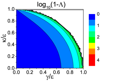
Figure 1: Strength $\Lambda$ of the sink versus the damping rate $\gamma$ and the coupling strength $\kappa$ in units of the exchange energy rate $\epsilon$.

The correlation function matrix $\langle\hat{\bf L}^{\rm id}(t)\hat{\bf L}^{{\rm id}\dagger{\rm T}}(t^{\prime})\rangle$ in Eq. (54) describes two coupled oscillators. Neglecting their coupling, both oscillators have identical eigenfrequencies expressed as $\tilde{\nu}_{\pm}=\gamma(-\kappa^{2}-\gamma^{2}\pm\sqrt{\mu^{4}+\epsilon^{2}\kappa^{2}})/\mu^{2}$. At least one eigenfrequency is negative and their sum gives the sink parameter $\Lambda$ written in Eq. (57). We note that, provided that the diagonal elements of the correlation function matrices of these oscillators were nonnegative, they describe the squeezed reservoirs [65]. If the squeezed reservoirs are considered the system dynamics qualitatively changes from the point of view of nonclassical and entangled states generation [66, 67]. Such states are obtained even for long times owing to the reservoir nonclassicality that is constantly being transferred into the system [66, 67, 68, 69, 70]. We also note that the nonclassical and entangled states emerge when nonlinear interactions with reservoirs are taken into account [71, 72].

A usual physical reservoir is composed of the populated modes whose random influence to the system compensates for the system loss (damping) or gain (amplification) of energy during its evolution. This means that there are nonnegative eigenvalues $\nu_{\pm}$, similarly as in the case of the original correlation functions in Eq. (2) [$\nu_{+}=2\gamma$, $\nu_{-}=0$]. Thus, the terms in the correlation function matrix $\langle\hat{\bf F}(t)\hat{\bf F}^{\dagger{\rm T}}(t)\rangle$ in Eq. (26), which are linearly proportional to time $t$, cannot be compensated by a suitable physical reservoir and, thus, the nonclassicality deterioration occurs inevitably during the evolution of the quantum $\mathcal{PT}$-symmetric system. This reflects the fundamental fact that whereas damping and amplification can compensate each other in (semi)classical coherent dynamics, the effects of fluctuating forces accompanying damping and amplification cannot be mutually suppressed.

Moreover, the complete omission of the Langevin forces $\hat{l}_{j}$ and $\hat{l}_{j}^{\dagger}$, $j=1,2$, results in a nonphysical behavior that violates the fluctuation-dissipation theorem. This situation corresponds to the semiclassical model described by the non-Hermitian Hamiltonian

$$\hat{H}^{\rm sc} = -i\gamma\hat{a}_{1}^{\dagger}\hat{a}_{1}+i\gamma\hat{a}_{2}^{\dagger}\hat{a}_{2}+\left[\epsilon\hat{a}_{1}^{\dagger}\hat{a}_{2}+\kappa\hat{a}_{1}\hat{a}_{2}+{\rm h.c.}\right].$$

We show in Secs. IV and V that the declinations of the system evolution from the physical one are qualitatively similar for both models.

IV Nonclassicality and entanglement in $\mathcal{PT}$-symmetric systems with different levels of reservoir fluctuations

A detailed role of the reservoir fluctuating forces in the evolution of nonclassical properties of two coupled oscillator modes is elucidated considering three models differently including reservoir fluctuations: (1) a physically-consistent model fully including reservoir fluctuations; (2) an ideal (sink) model with a partial inclusion of reservoir fluctuations obeying the fluctuation-dissipation relations and giving a periodic solution, and (3) a semiclassical model with no reservoir fluctuations thus violating the fluctuation-dissipation theorem.

We directly compare these three models for arbitrary values of all coefficients of the normal characteristic function in Eq. (59) below as well as by considering various properties of the modes. For simplicity, we restrict our attention to the initial coherent states in both oscillator modes. These states are Gaussian and they remain Gaussian during the evolution owing to the linear Heisenberg-Langevin equations in Eq.  (8). Their normal characteristic function $C_{\mathcal{N}}$ can be expressed as follows [54]:

$$C_{\cal N}(\mu_{1},\mu_{2},t) = \exp\Biggl{\{}\sum_{j=1,2}\Bigl{[}\left(\alpha_{j}^{*}(t)\mu_{j}-{\rm c.c.}\right)$$ (59)

$$\mbox{}-B_{j}(t)|\mu_{j}|^{2}+\left(C_{j}(t)\mu_{j}^{2*}+{\rm c.c.}\right)/2\Bigr{]}$$

$$\mbox{}+\left[D(t)\mu_{1}^{*}\mu_{2}^{*}+\bar{D}(t)\mu_{1}\mu_{2}^{*}+{\rm c.c.}\right]\Bigr{\}},$$

where c.c. stands for the complex conjugated term. Definitions of the time dependent parameters occurring in Eq. (59), as well as their simplified forms valid for the initial coherent states, are given as follows:

$$B_{j}(t) \equiv \langle\delta\hat{a}_{j}^{\dagger}(t)\delta\hat{a}_{j}(t)\rangle=\sum_{l=1,2}\left[|V_{jl}(t)|^{2}+\langle\hat{f}_{j}^{\dagger}(t)\hat{f}_{j}(t)\rangle\right],$$

$$C_{j}(t) \equiv \langle[\delta\hat{a}_{j}(t)]^{2}\rangle=\sum_{l=1,2}\left[U_{jl}(t)V_{jl}(t)+\langle[\hat{f}_{j}(t)]^{2}\rangle\right],$$

$$D(t) \equiv \langle\delta\hat{a}_{1}(t)\delta\hat{a}_{2}(t)\rangle$$

$$=\sum_{l=1,2}\left[U_{1l}(t)V_{2l}(t)+\langle\hat{f}_{1}(t)\hat{f}_{2}(t)\rangle\right],$$

$$\bar{D}(t) \equiv -\langle\delta\hat{a}_{1}^{\dagger}(t)\delta\hat{a}_{2}(t)\rangle$$ (60)

$$=-\sum_{l=1,2}\left[V_{1l}^{*}(t)V_{2l}(t)+\langle\hat{f}_{1}^{\dagger}(t)\hat{f}_{2}(t)\rangle\right],$$

where $\delta\hat{a}_{j}=\hat{a}_{j}-\langle\hat{a}_{j}\rangle$ for $j=1,2$.

We quantify the nonclassicality of the system using the Lee nonclassicality depth $\tau$ [73] derived from the threshold value $s_{\rm th}$ of the field-operator ordering parameter at which the corresponding quasi-distribution $\Phi_{s}$ of field amplitudes starts to behave as a classical function:

$$\tau=\frac{1-s_{\rm th}}{2}.$$ (61)

To arrive at the nonclassicality depth $\tau$, we first determine the characteristic function $C_{s}$ for an arbitrary ordering parameter $s$. The function $C_{s}$ keeps the Gaussian form of the normal characteristic function $C_{\cal N}$ with the following modified parameters [54]:

$$C_{s}(\mu_{1},\mu_{2},t)=\left.C_{\cal N}(\mu_{1},\mu_{2},t)\right|_{B_{j}\leftarrow B_{j,s}=(1-s)/2+B_{j},j=1,2}.$$ (62)

The quasi-distribution $\Phi_{s}$ associated to the characteristic function $C_{s}$ in Eq. (62) is obtained by the following Fourier transform:

$$\Phi_{s}(\alpha_{1},\alpha_{2},t) = \frac{1}{\pi^{2}}\prod_{j=1}^{2}\int d^{2}\mu_{j}\exp(\alpha_{j}\mu_{j}^{*}-\alpha_{j}^{*}\mu_{j})$$ (63)

$$\times C_{s}(\mu_{1},\mu_{2},t).$$

The existence of quasi-distribution $\Phi_{s}$ as an ordinary function requires a nonnegative determinant of the matrix ${\bf K}_{\Phi_{s}}$ of coefficients of the complex quadratic form occurring in the argument of the exponential function on the r.h.s. of Eq. (62):

$${\bf K}_{\Phi_{s}}=\frac{1}{2}\left[\begin{array}[]{cccc}-B_{1,s}&C_{1}^{*}&\bar{D}^{*}&D\\ C_{1}&-B_{1,s}&D^{*}&\bar{D}\\ \bar{D}&D&-B_{2,s}&C_{2}^{*}\\ D^{*}&\bar{D}^{*}&C_{2}&-B_{2,s}\end{array}\right].$$ (64)

For classical distributions $\Phi_{s}$ occurring for $s\leq s_{\rm th}$, all the four eigenvalues of the matrix ${\bf K}_{\Phi_{s}}$ are negative, which results in its positive determinant. At $s=s_{\rm th}$, one of these eigenvalues is zero and becomes positive for $s>s_{\rm th}$. Taking into account that the diagonal elements of the matrix ${\bf K}_{\Phi_{s_{\rm th}}}$ are given as $B_{j,s_{\rm th}}=(1-s_{\rm th})/2+B_{j}=\tau+B_{j}$, $j=1,2$, the nonclassicality depth $\tau$ is given as the greatest positive eigenvalue of the matrix ${\bf K}_{\Phi_{\cal N}}\equiv{\bf K}_{\Phi_{s=1}}$. Applications of these results can be found, e.g., in [74, 75, 76].

Applying this procedure to the characteristic function $C_{j,s}(\mu_{j},t)$ of mode $j$, we easily derive the following formula for the corresponding nonclassicality depth $\tau_{j}$:

$$\tau_{j}={\rm max}\{0,|C_{j}|-B_{j}\}.$$ (65)

Entanglement represents arguably the most striking manifestation of nonclassicality. Logarithmic negativity $E_{N}$ [77] is usually used to quantify it. For a two-mode Gaussian field with the characteristic function $C_{\cal N}$ given in Eq. (59), the negativity $E_{N}$ is determined from the coherence matrix $\sigma^{PT}$ belonging to the system with partially transposed mode 2 and, thus, defined for the vector $(\hat{q}_{1},\hat{p}_{1},\hat{q}_{2},-\hat{p}_{2})$ [78]:

$${\bf\sigma}^{PT} = \left[\begin{array}[]{cc}{\bf\sigma}_{1}&{\bf\sigma}_{12}^{PT}\\ \left[{\bf\sigma}_{12}^{PT}\right]^{T}&{\bf\sigma}_{2}^{PT}\end{array}\right],$$ (68)

$${\bf\sigma}_{1} = \left[\begin{array}[]{cc}1+2B_{1}+2\Re\{C_{1}\}&2\Im\{C_{1}\}\\ 2\Im\{C_{1}\}&1+2B_{1}-2\Re\{C_{1}\}\end{array}\right],$$ (71)

$${\bf\sigma}_{2}^{PT} = \left[\begin{array}[]{cc}1+2B_{2}+2\Re\{C_{2}\}&-2\Im\{C_{2}\}\\ -2\Im\{C_{2}\}&1+2B_{2}-2\Re\{C_{2}\}\end{array}\right],$$ (74)

$${\bf\sigma}_{12}^{PT} = 2\left[\begin{array}[]{cc}\Re\{D-\bar{D}\}&\Im\{-D+\bar{D}\}\\ \Im\{D+\bar{D}\}&\Re\{D+\bar{D}\}\end{array}\right],$$ (77)

where symbol $T$ stands for the transposed matrix. The partially transposed coherence matrix $\sigma^{PT}$ has two symplectic eigenvalues $\nu_{\pm}$ defined in terms of the invariants $\Delta={\rm det}\{{\bf\sigma}^{PT}\}$ and $\delta={\rm det}\{{\bf\sigma}_{1}\}+{\rm det}\{{\bf\sigma}_{2}^{PT}\}+2{\rm det}\{{\bf\sigma}_{12}^{PT}\}$ [78]:

$$\nu_{\pm}=\sqrt{\frac{\delta}{2}\pm\sqrt{\frac{\delta^{2}}{4}-\Delta}}.$$ (78)

The symplectic eigenvalue $\nu_{-}$ then determines the negativity $E_{N}$ along the formula:

$$E_{N}={\rm max}\{0,-\ln(\nu_{-})\}.$$ (79)

Considering the initial vacuum state in both modes and substituting the solution to the Heisenberg-Langevin equations given in Eqs. (18)—(26) into Eqs. (60) for the coefficients of the normal characteristic function $C_{\cal N}$, we arrive at the following formulas:

$$B_{1}(t) = \frac{\kappa^{2}}{2\mu^{2}}-\frac{\kappa^{2}}{2\mu^{2}}{\rm c}(t)-\frac{\epsilon^{2}\gamma}{2\mu^{3}}{\rm s}(t)+\frac{\epsilon^{2}\gamma}{\mu^{2}}t,$$

$$B_{2}(t) = \frac{\kappa^{2}+2\gamma^{2}}{2\mu^{2}}-\frac{\kappa^{2}+2\gamma^{2}}{2\mu^{2}}{\rm c}(t)+\frac{\epsilon^{2}\gamma}{2\mu^{3}}{\rm s}(t)+\frac{\epsilon^{2}\gamma}{\mu^{2}}t,$$

$$C_{1}(t) = C_{2}(t)=-\frac{\epsilon\kappa}{2\mu^{2}}+\frac{\epsilon\kappa}{2\mu^{2}}{\rm c}(t)+\frac{\epsilon\kappa\gamma}{2\mu^{3}}{\rm s}(t)-\frac{\epsilon\kappa\gamma}{\mu^{2}}t,$$

$$iD(t) = \frac{\kappa\gamma}{2\mu^{2}}-\frac{\kappa\gamma}{2\mu^{2}}{\rm c}(t)+i\frac{\kappa}{2\mu}{\rm s}(t),$$

$$i\bar{D}(t) = \frac{\epsilon\gamma}{2\mu^{2}}-\frac{\epsilon\gamma}{2\mu^{2}}{\rm c}(t)-\frac{\epsilon\gamma^{2}}{2\mu^{3}}{\rm s}(t)+\frac{\epsilon\gamma^{2}}{\mu^{2}}t,$$ (80)

where ${\rm s}(t)\equiv\sin(2\mu t)$ and ${\rm c}(t)\equiv\cos(2\mu t)$. The terms linearly proportional to time $t$ are apparent in Eq. (80). They disappear when the ideal reservoir is assumed. We note that similar linear time dependence of some physical quantities was observed in [52].

For comparison, we write the above coefficients for the semiclassical model in which the fluctuating forces are completely neglected:

$$B_{1}^{\rm sc}(t) = B_{2}^{\rm sc}(t)=\frac{\kappa^{2}}{2\mu^{2}}[1-{\rm c}(t)],$$

$$C_{1}^{\rm sc}(t) = C_{2}^{\rm sc}(t)=-\frac{\epsilon\kappa}{2\mu^{2}}[1-{\rm c}(t)],$$

$$D^{\rm sc}(t) = i\frac{\kappa\gamma}{2\mu^{2}}[1-{\rm c}(t)],$$

$$\bar{D}^{\rm sc}(t) = 0.$$ (81)

To assess the evolution of nonclassicality and entanglement, we determine the maximal values of the nonclassicality depths $\tau$ and the negativity $E_{N}$ in the first period of the periodical solutions found in the ideal (sink) model including partial reservoir fluctuations and the semiclassical model with no reservoir fluctuations:

$$\tau^{\rm max}=\max_{t\in\langle 0,2\pi/|\mu|\rangle}\{\tau(t)\},$$

$$E_{N}^{\rm max}=\max_{t\in\langle 0,2\pi/|\mu|\rangle}\{E_{N}(t)\}.$$ (82)

The extremal quantities defined in Eq. (82) are reasonable also for the physically-consistent model including complete reservoir fluctuations as, during the evolution, the level of noise in the system increases, which gradually conceals both nonclassicality and entanglement. Moreover, in the long-time limit of this model, the terms linearly proportional to time $t$ prevail. This results in a considerable simplification of the coefficients in Eq. (81):

$$B_{1}^{\infty}(t) = B_{2}^{\infty}(t)=\frac{\epsilon^{2}\gamma}{\mu^{2}}t,$$

$$C_{1}^{\infty}(t) = C_{2}^{\infty}(t)=-\frac{\epsilon\kappa\gamma}{\mu^{2}}t,$$

$$D^{\infty}(t) = 0,$$

$$\bar{D}^{\infty}(t) = -i\frac{\epsilon\gamma^{2}}{\mu^{2}}t.$$ (83)

Substitution of the long-time formulas in (83) into the matrix ${\bf K}_{\Phi_{\cal N}}$ leads to nonpositive eigenvalues. We note that the greatest eigenvalue is doubly degenerated and it is given by the formula $-B_{1}^{\infty}+\sqrt{|C_{1}^{\infty}|^{2}+|\bar{D}^{\infty}|^{2}}$. This means that the states are classical. Equations (65) and (79) for the nonclasicality depths $\tau_{j}$ of the modes and negativity $E_{N}$, respectively, confirm this:

$$\tau_{1}^{\infty}(t)=\tau_{2}^{\infty}(t)=\tau^{\infty}(t)=0,$$

$$E_{N}^{\infty}(t)=0.$$ (84)

We compare the predictions of the ideal (sink) model with partial reservoir fluctuations with those of the physically-consistent model with complete reservoir fluctuations at a general level by considering both nonclassicalities and entanglement. The maximal values of nonclassicality depths of the whole system ($\tau$) and its constituting modes ($\tau_{1}$, $\tau_{2}$), as well as the negativity $E_{N}$ are drawn in Fig. 2 as they depend on the system parameters.

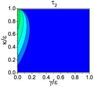
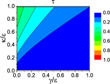
(a)                                  (b)                                  (c)                                  (d)

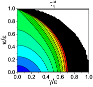
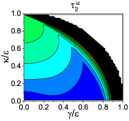
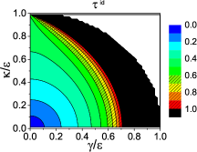
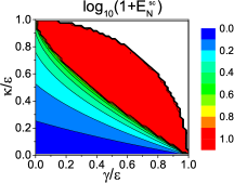
(e)                                  (f)                                  (g)                                  (h)

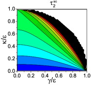
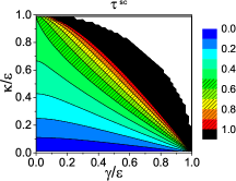
(i)                                  (j)                                  (k)                                  (l)

Figure 2: Nonclassicality depths $\tau_{1}$ of mode 1 (a,e,i), $\tau_{2}$ of mode 2 (b,f,j) and nonclassicality depths $\tau$ (c,g,k) and negativities $E_{N}$ (d,h,l) of the whole system versus dimensionless model parameters $\kappa/\epsilon$ and $\gamma/\epsilon$. Quantities with superscript id [sc] arise in the ideal (sink) model with partial reservoir fluctuations [semiclassical model with no reservoir fluctuations]. In the graphs with the nonclassicality depths, nonphysical values $\tau>1$ were determined in the black areas and values $\tau>0.5$ not compatible with the Gaussian states were reached in the hatched colored areas.

The comparison of graphs of the nonclassicality depths plotted in Figs. 2(e,f,g) for the ideal (sink) model with those in Figs. 2(a,b,c) for the physically-consistent model reveals that the nonclassicality depths $\tau^{\rm id}$, $\tau_{1}^{\rm id}$, and $\tau_{2}^{\rm id}$ of the ideal (sink) model are systematically greater than the nonclassicality depths $\tau$, $\tau_{1}$, and $\tau_{2}$ of the physically-consistent model with complete reservoir fluctuations. Moreover, whereas the physically-consistent model gives correct values of the nonclassicality depths even in the area of parameters with the exponential behavior, the ideal (sink) model predicts the nonclassicality depths only in the region of parameters with the oscillatory behavior. Even in this region, in the area close to the curve giving EPs, we find nonphysical values of the nonclassicality depths $\tau^{\rm id}$ greater than 1. The regions in which the ideal (sink) model gives the values of the nonclassicality depths $\tau^{\rm id}\leq 0.5$ compatible with the Gaussian form of the states are even smaller. The regions with $\tau^{\rm id}>0.5$ that contradict the Gaussian form of the states are indicated by the hatched colored areas in Figs. 2(e,f,g). Similarly, the values of the negativity $E_{N}^{\rm id}$ of the ideal (sink) model are plotted in Fig. 2(h). It is seen that they are systematically greater than those of the physically-consistent model with complete reservoir fluctuations in Fig. 2(d). In general, we may conclude that the ideal (sink) model, by partially suppressing the reservoir fluctuations, systematically enhances quantum features of the states in the system, as they manifest themselves in the nonclassicality depths and negativity.

In Figs. 2(i,j,k,l), we also plot the nonclassicality depths $\tau^{\rm sc}$, $\tau_{1}^{\rm sc}$, and $\tau_{2}^{\rm sc}$ together with the negativity $E_{N}^{\rm sc}$ of the semiclassical model with no reservoir fluctuations. The analysis of the behavior of this semiclassical model is very important, as such models are frequently addressed in the literature. The reason is that the omission of reservoir fluctuations allows to treat the model at the level of the non-Hermitian Hamiltonian description, which is considerably simpler than that based on the Liouvillian. The comparison of graphs in Figs. 2(i,j,k,l) with those in Figs. 2(a,b,c,d) determined for the physically-consistent model with complete reservoir fluctuations brings us to the conclusions similar to those made for the ideal (sink) model: The semiclassical model without reservoir fluctuations systematically overestimates both nonclassicality and entanglement quantifiers. On the other hand, a detailed comparison of the graphs in Figs. 2(i,j,k) with those in Figs. 2(e,f,g) reveals that the areas of parameters where the semiclassical model predicts the physically-acceptable values of the nonclassicality depths are larger than those belonging to the ideal (sink) model.

We note that, for experimental Gaussian fields, we may measure the principle squeezing variance [79] in homodyne detection [80] or even simpler by using photon-number-resolving detectors [81] to infer the values of the nonclassicality depth $\tau$. The negativity $E_{N}$ for a two mode field can then be conveniently obtained from photon-number-resolved measurements using photon-number moments up to fourth order [81].

V Comparison of the nonclassicality and entanglement evolution in $\mathcal{PT}$-symmetric systems with different levels of reservoir fluctuations

Differences observed in the extremal values of the nonclassicality and entanglement quantifiers in the ideal (sink) model with partial inclusion of reservoir fluctuations and the semiclassical model with no reservoir fluctuations vs. the physically-consistent model with complete reservoir fluctuations change/evolve in time. We may identify two qualitatively different types of their behavior. In the first one, the difference between the predictions for a given quantifier gradually increases with time, i.e., the relative difference develops from zero at the initial time. In this case the predictions of the investigated models with partial/no inclusion of reservoir fluctuations agree well with those of the physically-consistent model for short times and, as a rule of thumb, the longer is the time, the greater are the differences. In the second type of behavior, a nonzero difference of a given quantity occurs already at short times involving the initial time. There is no prediction for the subsequent evolution of this difference in this case and it may also decrease.

Both types of behavior are seen in Fig. 3, in which we plot the ratios of negativities $E_{N}/E_{N}^{\rm id}$ and $E_{N}/E_{N}^{\rm sc}$ and local nonclassicalities $\tau_{1}/\tau_{1}^{\rm id}$ and $\tau_{1}/\tau_{1}^{\rm sc}$ of mode 1 in the physically-consistent model vs. the ideal (sink) model and the semiclassical model, respectively, in three subsequent time instants $t_{1}=10^{-3}T$, $t_{2}=10^{-2}T$ and $t_{3}=10^{-1}T$. These instants represent small fractions of the period $T$,

$$T=2\pi/\sqrt{1-\frac{\kappa^{2}+\gamma^{2}}{\epsilon^{2}}},$$ (85)

that characterizes the periodic behavior of the models with partial/no inclusion of reservoir fluctuations.

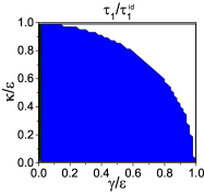
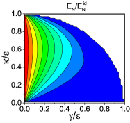
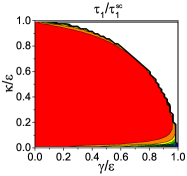
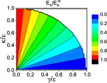
(a)                                  (b)                                  (c)                                  (d)

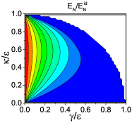
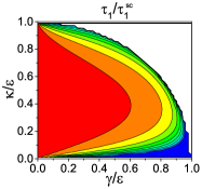
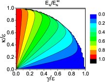
(e)                                  (f)                                  (g)                                  (h)

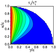
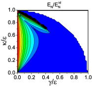
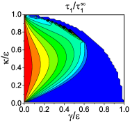
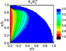
(i)                                  (j)                                  (k)                                  (l)

Figure 3: Ratios of nonclassicality depths $\tau_{1}/\tau_{1}^{\rm id}$ (a,e,i) and $\tau_{1}/\tau_{1}^{\rm sc}$ (c,g,k) of mode 1 and ratios of negativities $E_{N}/E_{N}^{\rm id}$ (b,f,j) and $E_{N}/E_{N}^{\rm sc}$ (d,h,l) of the whole system versus dimensionless model parameters $\kappa/\epsilon$ and $\gamma/\epsilon$. The ratios are determined for $t_{1}=10^{-3}T$ (a–d), $t_{2}=10^{-2}T$ (e–h) and $t_{3}=10^{-1}T$ (i–l) where $T$ is given in Eq. (85). Quantities with superscript id [sc] arise in the ideal (sink) model with partial reservoir fluctuations [semiclassical model with no reservoir fluctuations].

As the ideal (sink) and semiclassical models have partially or fully suppressed fluctuations, we expect greater values of the nonclassicality depths $\tau_{1}$ and the negativities $E_{N}$ arising in these models compared to those of the physically-consistent model. Indeed, the ratios plotted in Fig. 3 are smaller or equal to one for the vast majority of the system parameters. We note that the predictions of all the three models coincide for $\gamma/\epsilon=0$. Whereas the ratios of the negativities $E_{N}/E_{N}^{\rm id}$ and $E_{N}/E_{N}^{\rm sc}$ of both models with partial/no reservoir fluctuations and ratios of the nonclassicality depths $\tau_{1}/\tau_{1}^{\rm sc}$ of the semiclassical model start from 1 in the limit $t\rightarrow 0$, the ratios of the nonclassicality depths $\tau_{1}/\tau_{1}^{\rm id}$ of the ideal (sink) model are nonunit for very short times $t$. Comparing the graphs in Fig. 3 for time instants $t_{1}$, $t_{2}$, and $t_{3}$ (plotted in different rows), we observe the decrease of the ratios $E_{N}/E_{N}^{\rm id}$, $E_{N}/E_{N}^{\rm sc}$, and $\tau_{1}/\tau_{1}^{\rm sc}$ as the time increases. On the other hand, the ratio $\tau_{1}/\tau_{1}^{\rm id}$ being very small for very short times increases with time. We note that the physically-consistent model does not behave periodically owing to the constantly and irreversibly acting reservoir fluctuating forces. Nevertheless, the values of the nonclassicality depths $\tau_{1}$ and the negativities $E_{N}$ reached in the interval $\langle 0,T\rangle$, i.e., in the first period of the models with partial/no reservoir fluctuations, are usually greater than those obtained for longer times.

According to the fluctuation-dissipation theorem [56], the strength of the second-order correlation functions of the reservoir fluctuating forces depends linearly on the damping/amplification parameter $\gamma$. Thus, the greater is the ratio $\gamma/\epsilon$, (i) the stronger are the fluctuating forces, (ii) the more detrimental are the effects on the nonclassicality and entanglement, and (iii) the smaller are the ratios of the nonclassicality depths and negativities. This consideration valid for shorter times is documented in the graphs of Fig. 3. The ratio of the negativities $E_{N}/E_{N}^{\rm id}$ drawn in Fig. 3(j) for $t_{3}=10^{-1}T$ demonstrates departure from this rule valid for shorter times.

Fixing the ratio $\gamma/\epsilon$ and assuming again shorter times, the ratios of the negativities and nonclassicality depths in Fig. 3 attain maximum in the interval $\kappa/\epsilon\in\langle 0,\sqrt{1-\gamma^{2}/\epsilon^{2}}\rangle$. The increase of these ratios with the increasing $\kappa/\epsilon$ on the left-hand side of this maximum is attributed to the increase of the system nonlinearity. Greater values of the relative nonlinearity $\kappa/\epsilon$ mean faster nonclassicality and entanglement generation that prevails the detrimental role of the reservoir fluctuations. On the other hand, the decrease of these ratios on the right-hand-side of the maximum is attributed to the increased period $T$ (and, thus, the increased time instants $t_{1,2,3}$) with the increasing ratio $\kappa/\epsilon$ that brings longer action of the reservoir fluctuating forces.

The ratios of the negativities and nonclassicality depths are rather small in the area close to the curve for the EPs. This is a consequence of the fact that the period $T$ of the models with partial/no reservoir fluctuations is very long in this area and so the detrimental effect of reservoir fluctuations is strong. We note that the period $T$ goes to infinity at the EPs which results in the ratios determined at asymptotically long times.

These results obtained for specific time instants show, similarly as the results for maximal values of the nonclassicality depths and negativities in Sec. IV, that the applicability of the ideal (sink) model and the semiclassical model with partial/no inclusion of reservoir fluctuations for our predictions of the nonclassical properties of the studied ${\cal PT}$-symmetric system is rather limited. Whereas the semiclassical model gives reliable predictions for shorter times, some of the predictions of the ideal (sink) model may even be misleading at short times.

VI Conclusions

An analytical solution of the quantum-consistent $\mathcal{PT}$-symmetric model of two nonlinearly interacting damped and amplified bosonic modes coupled to reservoirs has been obtained. Using this solution the evolution of the nonclassicality and the entanglement of the generated Gaussian states has been analyzed in the whole space of model parameters. Whereas both nonclassical and entangled states are generated for shorter times, the reservoir fluctuations suppress their generation for long times. The analytical solution has allowed us to identify the reservoir noise contribution that increases linearly with time and causes a gradual loss of the nonclassicality and entanglement for long times.

To understand the origin of this degradation of the system ability to generate nonclassical and entangled states, we have considered two simplified models with a partial and full suppression of reservoir fluctuations: (1) a semiclassical model with no reservoir fluctuations and (2) an ideal (sink) model with a partial inclusion of reservoir fluctuations. Both models provide periodic solutions which allow for the generation of nonclassical and entangled states even for long times. The models differ by the level of their physical consistency: Whereas the semiclassical model violates the fluctuation-dissipation theorem, the ideal (sink) model obeys specific fluctuation-dissipation relations. However, its modified reservoir is endowed with the properties of the sink which removes the noise from the system.

Because of the partial or full suppression of reservoir fluctuations, both models provide systematically greater values of the nonclassicality depths as measures of quantumness and the negativity as a measure of entanglement. Unfortunately, the attained values of the nonclassicality depths may even exceed their physically allowed ranges, in the area of the model parameters around the EPs. Whereas the semiclassical model gives reliable predictions for short times, the ideal (sink) model, though being more physically consistent, may provide misleading results even for short times.

None of these two models, that allow for the generation of nonclassical and entangled states in quantum $\mathcal{PT}$-symmetric systems, can be applied to predict the system behavior for longer times. The only physically-consistent model is provided by the statistical physics of open quantum systems (using the Liouvillians or alternatively the Heisenberg-Langevin equations). This model properly includes the reservoir fluctuations associated with the damping and amplification of the system and, thus, describes its evolution in a physically consistent way. This model, however, shows that the irreversible reservoir fluctuations inevitably degrade the nonclassicality and entanglement generated in the system, which results in their complete loss for longer times. Thus, we find no possibility for mutual compensation of the reservoir fluctuations associated with the damping and amplification in the model. This limitation qualitatively differs from a direct action of the damping and amplification in the evolution of quantum $\mathcal{PT}$-symmetric systems, in which they mutually interfere to give a periodic evolution.

These results bring us to the general conclusion that the detrimental role of reservoir fluctuations in quantum $\mathcal{PT}$ -symmetric systems with damping and amplification cannot be avoided and the suppression of nonclassicality and entanglement in their evolution is their natural property that has to be accepted.