Generalizing Neural Wave Functions

Abstract

Recent neural network-based wave functions have achieved state-of-the-art accuracies in modeling ab-initio ground-state potential energy surface. However, these networks can only solve different spatial arrangements of the same set of atoms. To overcome this limitation, we present Graph-learned Orbital Embeddings (Globe), a neural network-based reparametrization method that can adapt neural wave functions to different molecules. Globe learns representations of local electronic structures that generalize across molecules via spatial message passing by connecting molecular orbitals to covalent bonds. Further, we propose a size-consistent wave function Ansatz, the Molecular Orbital Network (Moon), tailored to jointly solve Schrödinger equations of different molecules. In our experiments, we find Moon converging in 4.5 times fewer steps to similar accuracy as previous methods or to lower energies given the same time. Further, our analysis shows that Moon's energy estimate scales additively with increased system sizes, unlike previous work where we observe divergence. In both computational chemistry and machine learning, we are the first to demonstrate that a single wave function can solve the Schrödinger equation of molecules with different atoms jointly.

1 Introduction

In silico design of molecules requires accessing their quantum mechanical properties. This requires solving the associated Schrödinger equation. However, exact solutions are often intractable and approximations can become computationally expensive for larger and more complex systems. In recent years, neural network-based wave functions have emerged as a promising alternative, providing accurate and well-scaling approximation solutions in $O(N^{4})$ with the number of electrons $N$ (Hermann et al., 2022). Despite their theoretical scaling, this time complexity comes with a large prefactor leading to exploding computational requirements if one screens many different molecules. To address this limitation, Gao & Günnemann (2022) proposed the Potential Energy Surface Network (PESNet), a neural network wave function that generalizes across different structures. While reducing computational costs, PESNet is limited to different spatial arrangements of the same set of atoms.

A key challenge in the generalization to arbitrary molecules is the variable number of molecular orbitals. To resolve this, we introduce Graph-learned Orbital Embeddings (Globe), a generalization of PESNet that can solve arbitrary Schrödinger equations jointly. Like previous work, Globe uses a two-level approach where one network represents the electronic wave function and the other reparametrizes the wave function depending on the molecule. We resolve the issue of the dynamical numbers of molecular orbitals by embedding orbitals in 3D space. This enables us to learn local electronic structures via spatial message passing in graph neural networks (GNNs). For the wave function, we present the Molecular Orbital Network (Moon), the first size-consistent neural wave function. We accomplish size consistency in two key steps, firstly, by using spatial message passing Moon focuses on local interactions, and, secondly, by using the nuclei as anchor points for message passing. While the first step is strictly required for size consistency, the latter enables efficient reparametrization via Globe.

In our experiments, we find Moon accelerating convergence in joint training by up to 4.5 times and performing similarly to the attention-based PsiFormer on larger systems (von Glehn et al., 2023). Further, we observe that transfers of neural wave functions to larger structures do not require additional self-consistent field (SCF) calculations. In summary, our main contributions are:

• Globe, a reparametrization method for adapting neural wave functions to arbitrary molecules based on localized molecular orbital embeddings.

• Moon, a size-consistent neural wave function enabling generalization to larger structures, faster convergence, and accurate energies.

2 Background

Notation. We use the term molecule for a point cloud in $\mathbb{R}^{3}$ with charges assigned to each node. The term `geometry' refers to different spatial arrangements associated with the same set of charges. We use $N$ to denote the number of electrons and $M$ for the number of nuclei. ${\mathbf{r}}\in\mathbb{R}^{N\times 3}$ denotes a complete electron configuration whereas $\bm{r}\in\mathbb{R}^{3}$ denotes a single electron's position. For nuclei, we use ${\mathbf{R}}\in\mathbb{R}^{M\times 3}$ and ${\bm{R}}\in\mathbb{R}^{3}$, respectively. $Z_{m}$ denotes the charge of the $m$th nucleus. We use $[\phantom{a}]$ for the concatenation of vectors, $\circ$ for the Hadamard product, $\|x\|$ for the $L_{2}$-norm, bold capital letters ${\bm{A}}$ for matrices, bold lower case letters ${\bm{a}}$ for vectors, and normal face letters $a$ for scalars. Bracketed superscripts^(l) index sequences, e.g., layers in a neural network.

2.1 Quantum chemistry

At the heart of quantum chemistry is the Schrödinger equation. Its time-independent form is

$${\bm{H}}\psi=E\psi$$ (1)

where $\psi:\mathbb{R}^{N\times 3}\rightarrow\mathbb{R}$ is the electronic wave function, $E$ the energy and the Hamiltonian operator is

$${\bm{H}}= -\frac{1}{2}\sum_{n=1}^{3N}\nabla_{n}^{2}+V({\mathbf{r}}),$$ (2)

$$\begin{split}V({\mathbf{r}})=&\sum_{n>m=1}^{N}\frac{1}{\|r_{n}-r_{m}\|}-\sum_{n=1}^{N}\sum_{m=1}^{M}\frac{Z_{m}}{\|r_{n}-R_{m}\|}\\ &+\sum_{m>n=1}^{M}\frac{Z_{m}Z_{n}}{\|R_{m}-R_{n}\|},\end{split}$$ (3)

within the Born-Oppenheimer approximation, i.e., we approximate nuclei as particles with fixed positions. In linear algebra, Equation (1) is an eigenvalue problem where one wants to find the eigenfunction $\psi_{0}$ associated with the lowest eigenvalue $E_{0}$. These are commonly called the ground-state wave function and energy, respectively.

The electronic wave function $\psi$ describes the behavior of electrons. Note that electrons are not only specified by their spatial location $\bm{r}\in\mathbb{R}^{3}$ but also by their spin $\alpha\in\{\uparrow,\downarrow\}$. Though, since the spins do not occur in the Hamiltonian, they can be fixed a priori (Foulkes et al., 2001). For a function to be a valid wave function, it must satisfy two criteria. First, $\psi$ must obey the Fermi-Dirac statistics, i.e., it must be antisymmetric $\psi({\mathbf{r}})=\operatorname{sign}(\pi)\psi(\pi({\mathbf{r}}))$ w.r.t. permutations of same-spin electrons $\pi$. Second, the integral of its square must be one $\int\psi({\mathbf{r}})^{2}d{\mathbf{r}}=1$.

The challenge in computational chemistry is accurately approximating the ground-state energy. For instance, the total energy of a system can be decomposed into a mean-field energy and correlation energy, where the mean-field energy accounts for $\approx 99.5\%$ of the total energy. To reach chemical accuracy (typically defined as $1\text{\,}\mathrm{kcal}\text{\,}{\mathrm{mol}}^{-1}$), one has to accurately estimate $>99\%$ of the correlation energy, $>99.999\%$ of the total energy.

Most commonly, the wave function is represented by a determinant of molecular orbital functions (Slater, 1929):

$$\psi({\mathbf{r}})=\det\Phi, \Phi_{ij}=\phi_{j}(r_{i})$$ (4)

where the determinant ensures the antisymmetry w.r.t. permutations. The Hartree-Fock (HF) method provides a simple mean-field approximate solution to the Schrödinger equation where the molecular orbital functions $\phi^{\text{HF}}_{i}:\mathbb{R}^{3}\rightarrow\mathbb{R}$ are constructed with Linear Combinations of Atomic Orbitals (LCAO) $\varphi_{j}:\mathbb{R}^{3}\rightarrow\mathbb{R}$ (Lennard-Jones, 1929), $\phi^{\text{HF}}_{i}(x)=\sum_{m=1}^{M}\sum_{n=1}^{O_{m}}\omega_{i,m,n}\varphi_{m,n}(x)$ with $O_{m}$ being the number of atomic orbitals and $\varphi_{m,n}$ being the $n$th atomic orbital function of the $m$th atom, respectively. In matrix notation, Equation (4) can be written as

$$\psi({\mathbf{r}})=\det\Phi =\det(\varPhi\Omega^{T}) \varPhi,\Omega \in\mathbb{R}^{N\times\eta}$$ (5)

with $\eta=\sum_{m=1}^{M}O_{m}$, $\varPhi$ being a matrix of all atomic orbital functions evaluated at every electron position, and $\Omega$ being an optimized weight matrix.

2.2 Variational Monte Carlo

In Variational Monte Carlo (VMC), one approximates a solution to Equation (1) by picking a trial wave function $\psi_{\theta}$ parametrized by $\theta$ and iteratively minimizing the energy via gradient descent on $\theta$. Since the eigenfunctions of ${\bm{H}}$ are a complete basis, this variational optimization is an upper bound to the true ground-state energy. By reformulating Equation (1), one gets

$$E =\frac{\int\psi_{\theta}({\mathbf{r}}){\bm{H}}\psi_{\theta}({\mathbf{r}})d{\mathbf{r}}}{\int\psi^{2}_{\theta}({\mathbf{r}})d{\mathbf{r}}}$$ (6)

$$=\mathbb{E}_{{\mathbf{r}}\sim\psi^{2}_{\theta}}\left[\psi_{\theta}({\mathbf{r}})^{-1}{\bm{H}}\psi_{\theta}({\mathbf{r}})\right]=\mathbb{E}_{{\mathbf{r}}\sim\psi^{2}_{\theta}}\left[E_{\theta}({\mathbf{r}})\right].$$ (7)

In contrast to Equation (1), we here assumed an unnormalized wave function $\psi_{\theta}$, thus, the normalization factor. Further, we reformulate the integral in the second line using importance sampling. $E_{\theta}$ is the so-called local energy:

$$E_{\theta}({\mathbf{r}})= \psi_{\theta}({\mathbf{r}})^{-1}{\bm{H}}\psi_{\theta}({\mathbf{r}})$$ (8)

$$\begin{split}=&-\frac{1}{2}\sum_{i=1}^{3N}\left[\frac{\partial^{2}\log|\psi_{\theta}({\mathbf{r}})|}{\partial{\mathbf{r}}_{i}^{2}}+\frac{\partial\log|\psi_{\theta}({\mathbf{r}})|}{\partial{\mathbf{r}}_{i}}^{2}\right]\\ &+V({\mathbf{r}}).\end{split}$$ (9)

Finally, one optimize $\psi_{\theta}$ via gradient descent with

$$\nabla_{\theta}E =\mathbb{E}_{{\mathbf{r}}\sim\psi_{\theta}^{2}}\left[\left[E_{\theta}({\mathbf{r}})-\mathbb{E}_{{\mathbf{r}}\sim\psi_{\theta}^{2}}\left[E_{\theta}({\mathbf{r}})\right]\right]\nabla_{\theta}\log\psi_{\theta}({\mathbf{r}})\right]$$ (10)

where we estimate all expectations with Monte Carlo estimates using Metropolis-Hastings (Ceperley et al., 1977).

Due to the few constraints imposed on wave functions, recent works used neural networks to model them (Pfau et al., 2020; Hermann et al., 2020). In the neural network setting, learnable many-electron orbital functions $\phi_{i}:\mathbb{R}^{3}\times\mathbb{R}^{N\times 3}\rightarrow\mathbb{R}$ implemented by permutation equivariant neural networks replace the single-electron molecular orbital functions $\phi_{i}^{\text{HF}}$ in Equation (4).

3 Related Work

Traditional methods for modeling electronic wave functions have relied on Linear Combinations of Atomic Orbitals (LCAO) (Lennard-Jones, 1929) arranged in a Slater determinant (Slater, 1929). However, they cannot capture electron-electron interactions beyond a mean-field approximation. To address this issue, backflow transformations (Feynman & Cohen, 1956) and Jastrow factors (Jastrow, 1955) have been introduced. Later, Carleo & Troyer (2017) were the first to demonstrate the use of neural networks to model to quantum systems, though only for discrete spin systems. This approach has since been improved upon by using deep neural networks for real-space electronic systems (Han et al., 2019; Pfau et al., 2020; Hermann et al., 2020). In subsequent works, such neural networks have further refined (Gerard et al., 2022; von Glehn et al., 2023) and adopted to different settings like pseudopotentials (Li et al., 2022a), periodic systems (Wilson et al., 2022; Li et al., 2022b; Cassella et al., 2023) or diffusion Monte Carlo (DMC) (Wilson et al., 2021; Ren et al., 2022).

Despite their high accuracy, neural network-based wave function models are still inherently expensive for multiple systems. Two recent concurrent approaches addressed this challenge: DeepErwin, a weight-sharing method across geometries (Scherbela et al., 2022), and PESNet (Gao & Günnemann, 2022, 2023), a two-network approach that allows for joint training of several geometries, eliminating the need for retraining. But, while the former needs retraining for each structure, the latter is limited to different spatial arrangements of the same set of atoms.

4 Generalizing Neural Wave Functions

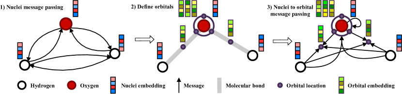
Figure 1: Globe steps. 1) Atom embeddings are obtained by message passing between atoms. 2) Orbital locations and embeddings are determined by core orbitals and molecular bonds. 3) Orbital embeddings are updated via a unidirectional message passing. For clarity, we omitted messages from each atom to each of the three core orbitals.

Compared to different geometries, generalization across different molecules comes with additional difficulties as the number of atoms, electrons, and orbitals change. To address these challenges, we identify two key desiderata that such a system should fulfill:

1. Invariance: A molecule's energy is invariant to Euclidean transformations and permutations. Thus, a generalizing wave function should result in invariant energy estimates. To achieve this, the wave function must be equivariant to Euclidean transformations and nuclei permutation (Gao & Günnemann, 2022).

2. Size consistency: As most quantum mechanical interactions happen within a short distance, a molecule's energy is an extensive quantity and scales additively with its size. For wave functions, this implies that the wave function decomposes into a product of the individual wave functions for distant molecules.

To incorporate Euclidean symmetries, we follow Gao & Günnemann (2022) by defining a PCA-based equivariant coordinate frame. Thus, in the following all references to the electron ${\mathbf{r}}$ and nuclei ${\mathbf{R}}$ positions are measured in the equivariant frame. To accomplish size consistency, the wave function must decompose into a product of two wave functions if two systems are sufficiently separated. In Appendix A, we show that decaying the value of molecular orbital functions $\phi_{i}$ to 0 far from the involved atoms is sufficient to implement this. We achieve this by relying on local interactions between pairs of particles (electrons/atoms) that exponentially decay with distance.

Like previous work, we adopt a two-network approach. While Moon represents the electronic wave function $\psi_{\theta}$, Globe acts solely on the nuclei and adapts the former's parameters to the molecule.

4.1 Graph-learned Orbital Embeddings (Globe)

Globe's task is to reparametrize the wave function depending on the molecular structure, i.e., it only acts on the atoms and does not consider electrons. To perform such a reparametrization, it must extract local electronic structure information from the atomic point cloud. Further, we must parametrize $N$ molecular orbital functions $\phi_{i}$, see Equation (4), which poses a challenge as their number depends on the number of electrons rather than atoms. As illustrated in Figure 1, we achieve both in a three-step procedure. First, we learn about atomic neighborhoods via message passing. Next, we localize orbitals and, finally, learn orbital embeddings via unidirectional message passing.

Message-passing network. Our message-passing network relies on the use of continuous filter convolutions (Schütt et al., 2018). We initialize the node embeddings by a charge embedding ${\bm{h}}^{\text{atom}(0)}_{i}={\bm{F}}^{\text{atom}}_{Z_{i}}$ and iteratively update them through message-passing as

$${\bm{h}}^{(l+1)}_{i} =f^{(l)}({\bm{h}}^{(l)}_{i},{\bm{m}}^{(l)}_{i}),$$ (11)

$${\bm{m}}^{(l)}_{i} =\frac{1}{\nu_{{\bm{R}}_{i}}^{\mathbf{R}}}\sum^{M}_{j=1}g^{(l)}({\bm{h}}^{(l)}_{i},{\bm{h}}^{(l)}_{j})\circ{\varGamma}^{(l)}({\bm{R}}_{i}-{\bm{R}}_{j}),$$ (12)

$$\nu_{x}^{\mathcal{N}} =1+\sum_{y\in\mathcal{N}}\exp\left(-\frac{\|x-y\|^{2}}{\sigma^{2}_{\text{norm}}}\right)$$ (13)

where $f^{(l)}$ and $g^{(l)}$ are implemented by MLPs, ${\varGamma}$ are spatial filters and $\nu$ is a spatial normalization with $\sigma_{\text{norm}}$ being a learnable parameter. By multiplying elementwise with spatial filters rather than concatenating with them, as done in Gao & Günnemann (2022), we decay long-range interactions between atoms and strengthen local interactions. Further, instead of averaging over all atoms, we normalize the message by a learnable normalization factor to account for the size of its neighborhood.

Spatial filters. To model arbitrary wave functions, we must break euclidean symmetries in our reparametrization (Gao & Günnemann, 2022). Previous work used positional encodings relative to the center of mass to achieve this. But, as the center of mass is an inherently global property, we instead break the symmetries in our spatial filters enforcing locality. Instead of being radial, our filters operate on the full three-dimensional space by constructing them as a Hadamard product of a Gaussian envelope and an MLP on the three-dimensional input:

$${\varGamma}^{(l)}({\bm{x}})= {\bm{W}}^{(l)}\beta({\bm{x}}),$$ (14)

$$\begin{split}\beta({\bm{x}})=&{\bm{W}}^{\text{env}}\left[\exp\left(-\left(\frac{\|{\bm{x}}\|}{\varsigma_{i}}\right)^{2}\right)\right]_{i=1}^{D}\\ &\circ\left({\sigma}\left({\bm{x}}{\bm{W}}^{(1)}+{\bm{b}}^{(1)}\right){\bm{W}}^{(2)}+{\bm{b}}^{(2)}\right)\end{split}$$ (15)

with $D$ being the number of envelope ranges $\varsigma_{i}$, and ${\sigma}$ being an activation function. While a combination of spherical harmonics and radial basis functions achieves similar symmetry breaking (Gasteiger et al., 2021; Zitnick et al., 2022), we found such freely learnable filters to perform better.

Orbital localization. A key challenge in adapting a wave function to arbitrary molecules is the molecular orbital functions $\phi_{i}$ as their number is not fully specified by the number of atoms but by the number of electrons. While generating one molecular orbital function per electron seems like an intuitive solution, this would cause two rows and columns in Equation (4) to permute if two electrons permute, resulting in a permutation symmetric rather than an antisymmetric function. Thus, the orbital functions must be independent of the actual electrons. One could generate the orbitals by a global graph embedding, e.g., via an RNN, but such a construction does not preserve locality and behaves unpredictably to changes in the nuclei.

We avoid such global constructions, by assigning each molecular orbital a location ${\bm{L}}_{i}\in\mathbb{R}^{3}$ and learning the parameters of the associated orbital function $\phi_{i}$ via message passing. To localize the orbitals, we distinguish between core and valence orbitals as core orbitals tend to interact little with other atoms (Foulkes et al., 2001). For each atom type, we define its valency by the number of bonds it can form, e.g., for hydrogen one, for carbon four, for oxygen two, etc. The number of core orbitals for the $i$th atom is then $\frac{Z_{i}-V_{i}}{2}$ with $V_{i}$ being the valency of the $i$th atom. These core orbitals are located at the same location as the nuclei. To determine the valence orbitals, we identify covalent bonds and locate the orbital in the center of that bond. We do this by iteratively picking the pairs of atoms closest to each other where each atom has at least one unpaired electron left. An example of our localized orbitals is depicted in Figure 1. In Appendix B, we provide a full definition of the algorithm.

While obtaining the orbital locations ${\bm{L}}_{i}$, we also define their types $T_{i}$. Where the order and the charge of the nucleus define the core orbital types, the bond's cardinality defines the valence orbital types. This categorial distinction avoids identical embeddings for two orbitals at the same location.

Orbital embedding. We initialize the orbital embeddings via their types ${\bm{h}}^{\text{o}(0)}_{i}={\bm{F}}^{\text{o}}_{T_{i}}$ and iteratively update them with an architecturally identical GNN as used for the atoms but with unidirectional message passing from the atoms to the orbitals. Here, we avoid bidirectional message passing as the orbital structure is wholly inferred from the nuclei and, thus, carries no additional geometric information.

Parameter estimation. Changes in a molecule's structure manifest in wave function parameters that depend either on atoms, orbitals, or a combination of both. Thus, Globe updates these parameters via their respective embeddings (${\bm{h}}^{\text{a}},{\bm{h}}^{\text{o}},{\bm{h}}^{\text{a-o}}$). Before generating parameters via individual MLPs, we pass them through shared MLPs and LayerNorms (Ba et al., 2016). To ensure that the wave function converges to a product for distant systems (Desiderata 2), we define atom-orbital embeddings as

$${\bm{h}}^{\text{a-o}}_{i,m}=\left[{\bm{h}}^{\text{a}(L)}_{m},{\bm{h}}^{\text{o}(L)}_{i}\right]{\bm{W}}\circ{\varGamma}^{\text{a-o}}({\bm{R}}_{m}-{\bm{L}}_{i}).$$ (16)

where the spatial filters vanish the contribution of the $m$th atom to the $i$th orbital with increasing distances.

4.2 Molecular Orbital Network (Moon)

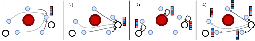
Figure 2: Illustration of Moon. 1) We initialize electron embeddings by aggregating their local neighborhood of electrons. 2) Nuclei aggregate electron embeddings via message passing. 3) Nuclei embeddings are iteratively updated. 4) Nuclei embeddings are structurally diffused towards the electrons via message passing. For clarity, we omitted most messages in 1), 2), and 4).

Moon represents the electronic wave function $\psi_{\theta}$, but, unlike previous work, Moon encourages local interactions via spatial message passing and avoids strong global interactions (Pfau et al., 2020; von Glehn et al., 2023). While PauliNet already represents a GNN-based wave function, it relies heavily on HF calculations and does not reach similar accuracy (Hermann et al., 2020; Gerard et al., 2022).

To avoid many expensive message-passing steps between electrons and nuclei, we simplify the message-passing structure. Figure 2 provides a conceptual overview of Moon. First, we encode the local electronic neighborhood for each electron. Next, nuclei aggregate electronic structure information. The nuclei embeddings are then iteratively updated and, lastly, diffused to the electrons. The basic functional form of Moon follows a Slater-Jastrow wave function

$$\psi_{\theta}({\mathbf{r}}) =\exp(J({\mathbf{r}}))\sum_{k=1}^{K}w_{k}\det\Phi^{k},$$ (17)

i.e., a product of a permutation invariant Jastrow factor and a weighted sum of Slater determinants. As Jastrow factor, we additively combine the Jastrow factors from Gao & Günnemann (2023) and von Glehn et al. (2023). In the following, we use bars $\bar{a}$ for atom parameters, tildes $\tilde{a}$ for orbital parameters, and both $\tilde{\bar{a}}$ for atom-orbital interaction parameters. These are the parameters that are updated through Globe. For clarity, we omit the Jastrow factor, residual connections, and normalization coefficient definitions here and refer the reader to Appendix C for detailed descriptions.

Embedding. As initial features, we use the pairwise distances between electrons and nuclei ${\bm{g}}^{\text{e-n}}_{ij}=[\bm{r}_{i}-{\bm{R}}_{j},\|\bm{r}_{i}-{\bm{R}}_{j}\|]$, and electron and electrons ${\bm{g}}^{\text{e-e}}_{ij}=[\bm{r}_{i}-\bm{r}_{j},\|\bm{r}_{i}-{\bm{R}}_{j}\|]$. As illustrated in Figure 2, we initialize the electron embeddings by a single electron-electron message-passing step

$${\bm{h}}^{\text{e}(0)}_{i} =\sum_{j=1}^{N}{\sigma}\left({\bm{g}}^{\text{e-e}}_{ij}{\bm{W}}^{\delta_{{\alpha}_{i}}^{{\alpha}_{j}}}\right)\circ{\varGamma}^{\delta_{{\alpha}_{i}}^{{\alpha}_{j}}}(\|\bm{r}_{i}-\bm{r}_{j})\|{\bm{W}}$$ (18)

where functions and matrices superscripted by the Kronecker delta $\delta_{{\alpha}_{i}}^{{\alpha}_{j}}$ indicate different weights. Here, we again use the spatial filters to decay interactions from far-apart particles. Like Gao & Günnemann (2022), we construct electron-nuclei interaction embeddings by combining electron embeddings ${\bm{h}}^{\text{e}(0)}_{i}$, nuclei embeddings $\bar{{\bm{z}}}_{m}$, and their distance ${\bm{g}}^{\text{e-n}}_{im}$ via

$${\bm{h}}^{\text{e-n}(0)}_{im} ={\sigma}\left({\bm{h}}^{\text{e}(0)}_{i}+\bar{{\bm{z}}}_{m}+{\bm{g}}^{\text{e-n}}_{im}\bar{{\bm{W}}}_{m}\right).$$ (19)

As the second step in Figure 2, these embeddings are then aggregated towards electrons and nuclei via spatial message passing while keeping separate embeddings for each spin state ${\alpha}\in\{\uparrow,\downarrow\}$ per nuclei:

$${\bm{h}}^{\text{n}{\alpha}(1)}_{m} =\sum_{i\in{\mathbb{A}}^{\alpha}}{\bm{h}}^{\text{e-n}}_{i,m}\circ\bar{{\varGamma}}_{m}^{\text{n}}(\bm{r}_{i}-{\bm{R}}_{m}),$$ (20)

$${\bm{h}}^{\text{e}(1)}_{i} =\sum_{m=1}^{M}{\bm{h}}^{\text{e-n}}_{i,m}\circ\bar{{\varGamma}}_{m}^{\text{e}}(\bm{r}_{i}-{\bm{R}}_{m})$$ (21)

where ${\mathbb{A}}^{\alpha}$ is the index set of electrons with spin ${\alpha}$ and $\bar{{\varGamma}}$ being the spatial filters from Equation (14) with atom-parameters, see Appendix C. By using message passing instead of concatenation as commonly done in single-molecule works (von Glehn et al., 2023), we achieve invariance to nuclei permutations, see Desiderata 1 in Section 4.

Update. We iteratively update the nuclei embeddings

$${\bm{h}}^{\text{n}{\alpha}(l+1)}_{m} ={\bm{h}}^{\text{n}{\alpha}(l)}_{m}+{\sigma}([{\bm{h}}^{\text{n}{\alpha}(l)}_{m},{\bm{h}}^{\text{n}\hat{{\alpha}}(l)}_{m}]{\bm{W}}^{(l)}+{\bm{b}}^{(l)})$$ (22)

where $\hat{{\alpha}}$ denotes the opposing spin of ${\alpha}$. For efficiency reasons, we do not perform message passing between nuclei here as we found it to have no significant impact.

Diffusion. After $L$-many update steps, a single message-passing step diffuses the nuclei embeddings to the electrons

$${\bm{h}}^{\text{e}(L)}_{i} ={\sigma}({\bm{h}}^{\text{e}(0)}_{i}{\bm{W}}+{\bm{m}}_{i}),$$ (23)

$$\begin{split}{\bm{m}}_{i}&=\sum_{m=1}^{M}\left(\left[{\bm{h}}^{\text{n}{\alpha}_{i}(L)}_{m},{\bm{h}}^{\text{n}\hat{{\alpha}}_{i}(L)}_{m}\right]{\bm{W}}+{\bm{b}}\right)\\ &\phantom{=}\circ\bar{{\varGamma}}_{m}^{\text{diff}}(\bm{r}_{i}-{\bm{R}}_{m})\end{split}$$ (24)

with ${\alpha}_{i}$ denoting the spin of the $i$th electron. The spatial filters in this step enable the network to learn different directional messages which are important in modeling directional wave functions, e.g., the excited states of the hydrogen atom.

Orbital construction. After diffusion, we construct restricted orbitals like Gao & Günnemann (2023) with adaptive orbital and envelope parameters:

$$\begin{split}\phi^{k}_{i}(\bm{r}_{j})=&\left((\tilde{w}_{i}^{k\delta_{{\alpha}_{i}}^{{\alpha}_{j}}})^{T}{\bm{h}}^{\text{e}(L)}_{j}+\tilde{b}_{j}^{k\delta_{{\alpha}_{i}}^{{\alpha}_{j}}}\right)\\ &\sum_{m=1}^{M}\tilde{\bar{\pi}}_{im}^{k\delta_{{\alpha}_{i}}^{{\alpha}_{j}}}\exp(-\tilde{\bar{\sigma}}^{k\delta_{{\alpha}_{i}}^{{\alpha}_{j}}}_{im}\|\bm{r}_{j}-{\bm{R}}_{m}\|).\end{split}$$ (25)

Here, the exponential envelope from Spencer et al. (2020) guarantees that our wave function will have a finite integral. In Appendix C, we describe how we restrict the envelope parameters $\sigma$ such that we fulfill size consistency desiderata.

4.3 Optimization

We train the whole network end-to-end in a two-step procedure. We first pretrain the orbitals $\phi_{i}$ on HF solutions and, next, perform variational optimization (Pfau et al., 2020).

Pretraining. Pretraining is important to ensure a stable variational optimization (Pfau et al., 2020; von Glehn et al., 2023). Traditionally, one would match the neural network's orbitals $\phi_{i}$ with those of an HF solution $\phi^{\text{HF}}_{i}$. But, with our localized orbitals this may cause a mismatch between nuclei involved in the $i$th neural orbital function and HF orbital function as the HF solution is typically sorted by energy state rather than locality. We resolve this issue by noticing that the HF wave function does not change if one multiplies the orbital matrix $\Phi=\varPhi\Omega^{T}$ by a matrix ${\bm{A}}$ with unit determinant, i.e., $\psi({\mathbf{r}})=\det(\varPhi\Omega^{T})=\det(\varPhi\Omega^{T}{\bm{A}})$. With this in mind, we can find a matrix ${\bm{A}}$ such that the new coefficient matrix $\hat{\Omega}^{T}=\Omega^{T}{\bm{A}}$ enforces locality. We describe this optimization procedure in Appendix D. After finding $\hat{\Omega}^{T}$, we perform traditional pretraining by matching the neural network orbitals to the localized HF orbitals. To avoid overfitting, we add a regularization loss on the outputs of the reparametrization network detailed in Appendix E.

Variational optimization. Like Gao & Günnemann (2022), we train both the wave function and the reparametrization network end-to-end and precondition the VMC gradients with natural gradient descent. But, since we deal with molecules of varying sizes unlike previous work, the gradients obtained from the different molecules may vary by orders of magnitude (like their energy). To avoid larger molecules from dominating the gradients, we rescale the gradients based on the standard deviation of the local energies associated with the molecule. We discuss this rescaling in Appendix F and the full VMC optimization in Appendix G.

4.4 Limitations

While Globe can learn a generalized wave function across different geometries of molecules, there are limitations. Firstly, despite having a rotation equivariant wave function, Globe is not smooth under arbitrary geometric perturbations. For instance, changes that cause the equivariant frame from Gao & Günnemann (2022) to flip result in discrete changes in the wave function, similar discontinuities may happen to our orbital localization as discussed in Appendix B. The coordinate frame also breaks the size-consistency of Moon as the frames of the two molecules do not necessarily align anymore. These are general issues introduced by natural symmetries that one must break to model arbitrary wave functions. Secondly, while we found our gradient rescaling based on the energy's standard deviation easing optimization, we found it to be insufficient if the discrepancy between molecules is large. For instance, if one trains a hydrogen-based system jointly with heavier atoms like nitrogen we found the optimization resulting in worse results than one obtains from training solely on the hydrogen-based system. Lastly, in its current state, the number of electrons is equal to the sum of atomic charges, and the number of spin-up and down electrons may differ by at most 1, prohibiting modeling ionic systems.

5 Experiments

Here, we analyze Globe and Moon across a variety of different experimental settings. Firstly, we investigate the behavior of Globe when training on similar geometries where one would expect significant information overlap between molecular orbitals. Next, we take a look at its extrapolation behavior on such similar structures. Thirdly, we train Globe on molecules that share no common structure. Fourthly, we investigate the transferability of a trained Globe to similar and larger molecules. Lastly, we compare Moon with recent neural wave functions on the larger benzene molecule.

As the true ground-state energies for any molecular system are rarely known, we either compare them to highly accurate reference calculations or report variational energies or their standard deviation. As discussed in Section 2, VMC energies are upper bounds to the true energy and, thus, lower is better. Further, as the wave function approaches the ground state, the standard deviation of the local energy approaches zero providing a proxy for the convergence to the ground state. Appendix H details the setup and Appendix I lists the geometries we used in the following. Timings and model sizes can be found in Appendix J and Appendix K. Appendix L provides a model size ablation.

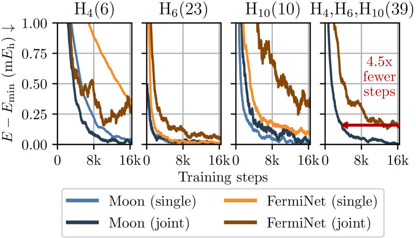
Figure 3: Convergence plots of Globe with Moon and FermiNet. Numbers in brackets show the number of geometries per molecule. In joint training, Moon converges 4.5 times faster and to lower energies.

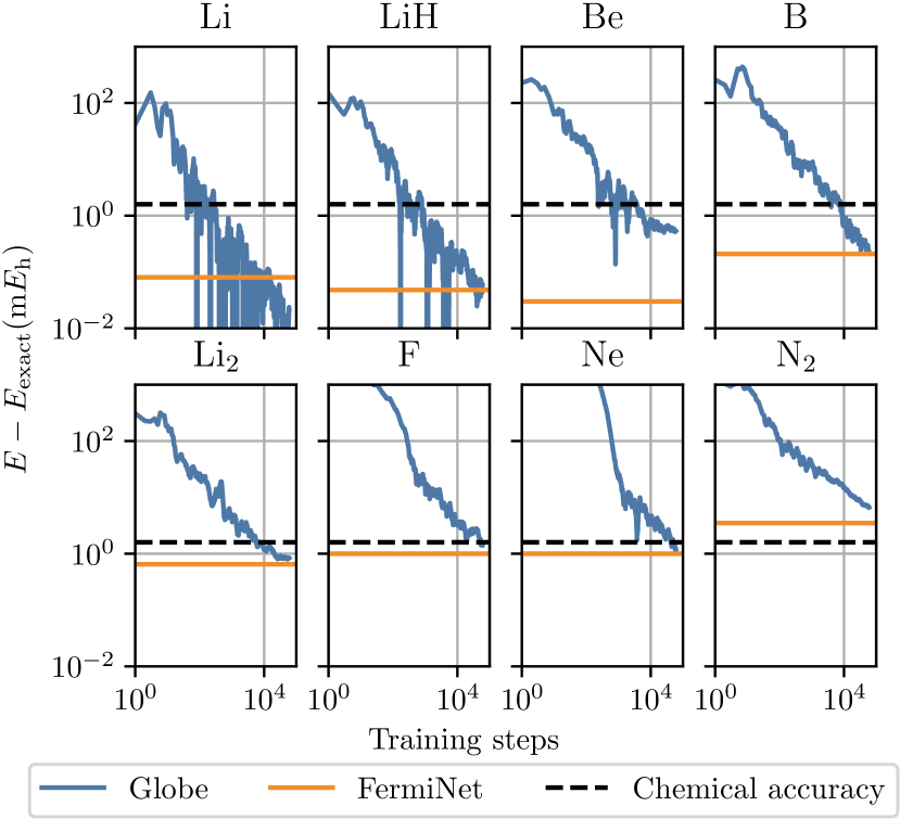
Figure 4: Globe trained on different structures jointly. FermiNet is optimized per molecule, numbers are taken from Pfau et al. (2020). Globe reaches chemical accuracy everywhere except N₂ where the specially optimized FermiNet also fails.

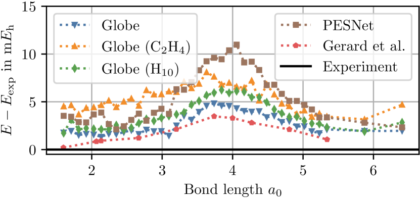
Figure 5: Relative error to Le Roy et al. (2006) on the N₂ potential energy surface. For Globe, the brackets show the additional molecule that the network has trained on. The hydrogen chain H₁₀ and ethene result in $0.96\text{\,}\mathrm{m}\mathrm{\text{$E_{\textup{h}}$}}{}$ and $2.71\text{\,}\mathrm{m}\mathrm{\text{$E_{\textup{h}}$}}{}$ higher energies.

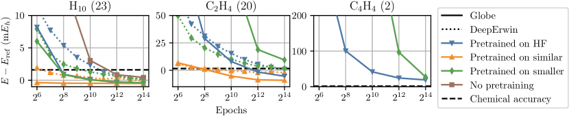
Figure 6: Average energy difference to reference data by training epochs for Globe and DeepErwin across three molecules with different pretraining techniques. Bracketed numbers show the number of geometries. For cyclobutadiene, we neither have DeepErwin reference numbers nor did we run the transferability experiment from similar structures. On ethene and cyclobutadiene, models without any pretraining are not visible due to their high error, see Appendix O.

Learning on similar systems. Training on similar systems jointly may be useful in several settings, e.g., in binding energy computations (Trogolo et al., 2019) or in labeling a diverse dataset (Hoja et al., 2021). Two key aspects are of interest here. Firstly, we investigate the loss in accuracy when training on different molecules and, secondly, we compare Moon to the existing FermiNet (Pfau et al., 2020) to identify potential benefits in convergence and accuracy. For FermiNet, we include all improvements from Gao & Günnemann (2023) and the Jastrow factor from von Glehn et al. (2023). As systems, we choose the hydrogen rectangle H₄, the 6-element hydrogen chain H₆, and the 10-element hydrogen chain H₁₀. Note that each of these systems is a collection of different geometries. We train each wave function model with our reparametrization network on four different settings, one for each molecule and one where we train on all of them jointly. Due to the variational principle, lower energies are better.

Figure 3 shows the average energy during training for both FermiNet and Moon in their two training settings (joint optimization, single molecule only). One can see that Moon converges strictly faster than a similar-sized FermiNet. For small systems, we observe that joint training even accelerates convergence in terms of steps. For FermiNet, we observe a significant gap between single and joint training for the larger hydrogen chain while Moon converges to the same energy in both regimes. Importantly, we observe that Moon behaves significantly more stable in joint optimization compared to FermiNet. We compare the standard deviation of the energy during training in Appendix M.

Table 1: Comparison between Moon and FermiNet in solving separated hydrogen chains. H₁₀ indicates the energy of a single hydrogen chain, H₁₀ + H₁₀ for two hydrogen chains $100\text{\,}\mathrm{a_{0}}$ apart, and $\Delta$ indicates the difference in energy between twice the energy of single chain compared to solving both systems jointly. All values are in Hartree.

	H10	H10 + H10	2 $\times$ H10	$\Delta$
FermiNet	-5.6631	-10.7564	-11.3262	-0.5698
Moon	-5.6632	-11.3264	-11.3264	0.0000

Size consistency. As discussed in Desiderata 2 in Section 4, for distant molecules the joint wave function is equal to the product of the individual wave functions. In contrast to previous neural wave functions like FermiNet, Globe and Moon adhere to this limit case. We demonstrate this by training Globe with FermiNet and Moon on the hydrogen chain H₁₀ and transfer the wave function to two separated hydrogen chains $100\text{\,}\mathrm{a_{0}}$ apart. As an optimal result, one expects the energy of the distant hydrogen chains to be equal to twice the energy of a single chain.

In Table 1 we list the difference between these settings. While FermiNet leads to a significant error of $570\text{\,}\mathrm{m\text{$E_{\textup{h}}$}}$, Moon's result is in perfect agreement with the desiderata. In closer regimes, we analyze the extensivity of FermiNet and Moon in Appendix N.

Learning on dissimilar systems. While optimizing similar molecules has a small impact on the performance of Globe, we now analyze how unrelated molecules affect final energies. We test this by solving for the ground-state energies of various small systems jointly. We pick Li, LiH, Be, B, Li₂, F, Ne, and N₂ from Pfau et al. (2020) as the dataset.

In Figure 4, one sees the energy for each system during training. While, for small systems, Globe with Moon accomplishes lower energies than FermiNet despite training jointly, we observe that this does not carry over to larger systems where the gap between both increases. For all molecules, except for N₂ where FermiNet also fails to reach chemical accuracy, Globe's energies are within the chemical accuracy of the true energy. To close the gap to FermiNet, we found that increasing the size of the wave function Moon has a significant impact on the final energy. We investigate this in Appendix L and argue that this is due to the increased capacity requirement in capturing many wave functions within a single model.

Learning dissimilar energy surfaces. While the previous paragraph analyzed the absolute energies in training on different molecules, here we look at the consistency of energy surfaces when training on different energy surfaces jointly. To test this, we train three Globe on the nitrogen dimer (N₂), once solely on nitrogen, once with the hydrogen chain (H₁₀) as a smaller molecule, and once with ethane (C₂H₄) as a larger molecule. We chose the nitrogen dimer due to its challenging nature (Pfau et al., 2020). Further, we compare Globe to recent neural network-based solutions (Gerard et al., 2022; Gao & Günnemann, 2022).

The potential energy surface in Figure 5 shows that Globe comes close to the performance of current state-of-the-art neural wave functions while being able to model different molecules jointly. We suspect the gap to Gerard et al. (2022) is due to the lower number of determinants, as we use 16 instead of 32 since Pfau et al. (2020) found these to be an important hyperparameter for the nitrogen dimer. Though, one can see that adding unrelated molecules to the optimization worsens the final results depending on the system sizes. For instance, adding the relatively low-energy hydrogen chain worsens the results by $0.96\text{\,}\mathrm{m\text{$E_{\textup{h}}$}}$, and the larger ethene structures lead to $2.71\text{\,}\mathrm{m\text{$E_{\textup{h}}$}}$ worse energies on average. Note that the models trained with dissimilar structures also have seen fewer nitrogen samples during training as we evenly divide the total batch size of 4096 across all molecules.

Transferibility. Here, we analyze the transferability of Globe across different molecules. Like Scherbela et al. (2022), we train Globe on several molecules and transfer the wave function either to different geometries, or larger molecules. Specifically, we use the 10-element hydrogen chain (H₁₀), ethene (C₂H₄), and cyclobutadiene (C₄H₄). As smaller molecules, we use the 6-element hydrogen chain (H₆), methane (CH₄), and ethene, respectively. We compare our results to DeepErwin (Scherbela et al., 2022). Though, there are key distinctions in our setups. While Globe optimizes all molecules at once, DeepErwin optimizes each molecule independently with weight-sharing applied between the wave functions. Further, DeepErwin performs new CASSCF calculations for each molecule while we apply Globe without any SCF calculations to the new molecule. An epoch for DeepErwin is one optimization step per molecule with a batch size of 2048 per molecule. Since we optimize all geometries jointly, an epoch is a single step for us with a batch size of 4096 shared for all molecules in the batch. Thus, we trained Globe with approximately 10 times fewer samples and 20 times fewer steps.

The convergence plots in Figure 6 show that Globe generally converges quickly to within chemical accuracy in the hydrogen chain and ethene for the standard setting, i.e., pretraining from HF. For cyclobutadiene, we suspect the gap to Gao & Günnemann (2023) is due to our smaller wave function, i.e., we use an embedding dim of 256 and 16 determinants instead of 512 and 32, respectively. Consistent with the results from Scherbela et al. (2022), we find starting from smaller molecules generally worsens convergence for larger systems. Still, pretraining on smaller molecules leads to similar results given sufficient training steps and outperforms the models without pretraining. For a view of the full convergence diagram, see Appendix O. Notably, we observe convergence without performing a single HF calculation on the larger structures, which was essential for previous methods (Pfau et al., 2020; Scherbela et al., 2022). Compared to DeepErwin, Globe results in $0.6\text{\,}\mathrm{m\text{$E_{\textup{h}}$}}$ and $6.3\text{\,}\mathrm{m\text{$E_{\textup{h}}$}}$ lower energies for the hydrogen chain and ethene, respectively.

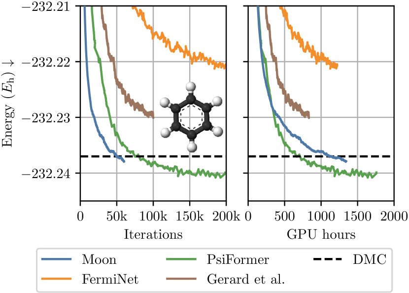
Figure 7: Energy during optimization on benzene (C₆H₆) by iterations and GPU hours. Reference data is taken from von Glehn et al. (2023); Gerard et al. (2022); Ren et al. (2022). Energies are averaged over 4000 iterations. Moon shows similar convergence behavior to the attention-based PsiFormer.

Larger systems. As neural-network solutions are interesting thanks to their theoretical scaling, we investigate how Moon scales to larger systems compared to FermiNet (Pfau et al., 2020), recent improvements to FermiNet (Gerard et al., 2022), diffusion Monte Carlo (DMC) calculations (Ren et al., 2022), and the recently proposed attention-based PsiFormer (von Glehn et al., 2023). As system, we use the benzene molecule (C₆H₆), as recent work found a large gap between VMC and the true ground-state energy (Ren et al., 2022; von Glehn et al., 2023).

Figure 7 plots the energy of the system throughout training by iterations and GPU hours. Note that FermiNet, PsiFormer, and Gerard et al. (2022) were optimized with KFAC (Martens & Grosse, 2015) while Moon uses CG-based natural gradient descent. While CG-based natural gradient descent leads to faster early convergence, KFAC results in similar update steps later in training while being two to three times faster per iteration. In energy, we find Moon to behave similarly to PsiFormer in that it approaches lower than DMC energy levels. Compared to the best FermiNet results, we find Moon to reach similar energies in 3 times fewer GPU hours and converge in an identical time to $13.5\text{\,}\mathrm{m\text{$E_{\textup{h}}$}}$ lower energies.

6 Conclusion

Solving many Schrödingers jointly with a single system holds the promise of learning generalizing wave functions. Like recent deep learning-based density functional theory (DFT) functionals (Snyder et al., 2012; Kirkpatrick et al., 2021), learning a general neural network solution for quantum mechanical calculations may accelerate material discovery while increasing accuracy. In this work, we introduced Globe, the first systematic approach to performing such a generalization. By embedding orbitals as points in space and using message passing, we can learn dynamic numbers of molecular orbital functions for different molecules. Further, we presented a novel locality-driven wave function, Moon, that shows significant improvements in convergence and extensivity than previous methods when trained on diverse molecules. With Globe and Moon, we are the first to demonstrate the solving of Schrödinger equations of different molecules within a single wave function.

Acknowledgements. We greatly thank Chendi Qian for his valuable early work on designing wave functions and Michael Scherbela for swiftly sharing their data and results with us. Further, we would like to thank Tom Wollschläger and Marten Lienen for their discussion on the localization algorithm, and Jan Schuchardt and Yan Scholten for their invaluable feedback on the paper.

Funded by the Federal Ministry of Education and Research (BMBF) and the Free State of Bavaria under the Excellence Strategy of the Federal Government and the Länder.

Appendix A Size consistency in quantum chemistry

If one is given two distant molecules, one can show that the Hamiltonian ${\bm{H}}$ from Equation 1 decomposes into two Hamiltonians ${\bm{H}}_{1},{\bm{H}}_{2}$ for each of the respective systems.

W.l.o.g., let the electrons be sorted such that ${\mathbf{r}}=[{\mathbf{r}}_{1},{\mathbf{r}}_{2}]\in\mathbb{R}^{N},{\mathbf{r}}_{1}\in\mathbb{R}^{N_{1}},{\mathbf{r}}_{2}\in\mathbb{R}^{N_{2}}$. First, one rewrites the full Hamiltonian

$$\begin{split}{\bm{H}}=&-\frac{1}{2}\sum_{n=1}^{3N}\nabla_{n}^{2}\\ &+\sum_{n>m=1}^{N}\frac{1}{\|r_{n}-r_{m}\|}-\sum_{n=1}^{N}\sum_{m=1}^{M}\frac{Z_{m}}{\|r_{n}-R_{m}\|}\\ &+\sum_{m>n=1}^{M}\frac{Z_{m}Z_{n}}{\|R_{m}-R_{n}\|},\end{split}$$ (26)

in terms of the Hamiltonians of the individual systems ${\bm{H}}_{1},{\bm{H}}_{2}$

$$\begin{split}{\bm{H}}=&{\bm{H}}_{1}+{\bm{H}}_{2}+\sum_{n\in{\mathbb{B}}_{1}}\sum_{m\in{\mathbb{B}}_{2}}\frac{1}{\|\bm{r}_{n}-\bm{r}_{m}\|}\\ &-\sum_{n\in{\mathbb{B}}_{1}}\sum_{m\in{\mathbb{A}}_{2}}\frac{Z_{m}}{\|\bm{r}_{n}-{\bm{R}}_{m}\|}\\ &-\sum_{n\in{\mathbb{B}}_{2}}\sum_{m\in{\mathbb{A}}_{1}}\frac{Z_{m}}{\|\bm{r}_{n}-{\bm{R}}_{m}\|}\\ &+\sum_{n\in{\mathbb{A}}_{1}}\sum_{m\in{\mathbb{A}}_{2}}\frac{Z_{m}Z_{n}}{\|\bm{r}_{n}-{\bm{R}}_{m}\|}.\end{split}$$ (27)

where ${\mathbb{A}}_{1},{\mathbb{A}}_{2}$ and ${\mathbb{B}}_{1},{\mathbb{B}}_{2}$ are the index sets for the nuclei and electrons for both systems, respectively. For distant systems, $\frac{1}{\|\bm{r}_{n}-\bm{r}_{m}\|}\approx\frac{1}{\|\bm{r}_{n}-{\bm{R}}_{m}\|}\approx\frac{1}{\|{\bm{R}}_{n}-{\bm{R}}_{m}\|}$:

$$\begin{split}{\bm{H}}=&{\bm{H}}_{1}+{\bm{H}}_{2}+c(\\ &\underbrace{\phantom{-}\sum_{n\in{\mathbb{B}}_{1}}\sum_{m\in{\mathbb{B}}_{2}}1-\sum_{n\in{\mathbb{B}}_{1}}\sum_{m\in{\mathbb{A}}_{2}}Z_{m}}_{=0}\\ &\underbrace{-\sum_{n\in{\mathbb{B}}_{2}}\sum_{m\in{\mathbb{A}}_{1}}Z_{m}+\sum_{n\in{\mathbb{A}}_{1}}\sum_{m\in{\mathbb{A}}_{2}}Z_{m}Z_{n}}_{=0}).\end{split}$$ (28)

where $c=\frac{1}{\|{\bm{R}}_{n}-{\bm{R}}_{m}\|},n\in{\mathbb{A}}_{1},m\in{\mathbb{A}}_{2}$. One may notice that for non-ionic systems $|{\mathbb{B}}_{i}|=\sum_{m\in{\mathbb{A}}_{i}}Z_{m}$. Thus, the first two and the last two sums cancel out and one is left with the sum of the individual Hamiltonians.

Given the decomposition of the Hamiltonian, one can show that the lowest eigenvalue of ${\bm{H}}$ is $E_{1}+E_{2}$ where $E_{1}$ and $E_{2}$ are the lowest eigenvalues associated with the eigenfunctions $\psi_{1}$ and $\psi_{2}$ of ${\bm{H}}_{1}$ and ${\bm{H}}_{2}$, respectively:

$${\bm{H}}(\psi_{1}\psi_{2}) =({\bm{H}}_{1}+{\bm{H}}_{2})(\psi_{1}\psi_{2})$$ (29)

$$={\bm{H}}_{1}\psi_{1}\psi_{2}+{\bm{H}}_{2}\psi_{2}\psi_{1}$$ (30)

$$=E_{1}\psi_{1}\psi_{2}+E_{2}\psi_{2}\psi_{1}$$ (31)

$$=(E_{1}+E_{2})\psi_{1}\psi_{2}.$$ (32)

Thus, the ground state wave function of the combined Hamiltonian ${\bm{H}}$ is the product of the individual ground state wave functions $\psi_{1}$ and $\psi_{2}$.

To obtain the decomposition $\psi=\psi_{1}\psi_{2}$, it remains to show that the molecular orbital functions $\phi$ must only act on close-by electrons, i.e.,

$$\phi_{n}(\bm{r}_{m}|{\mathbf{r}})=\begin{cases}\phi_{n}(\bm{r}_{m}|{\mathbf{r}}_{{\mathbb{B}}_{1}})&\text{if }n,m\in{\mathbb{B}}_{1},\\ \phi_{n}(\bm{r}_{m}|{\mathbf{r}}_{{\mathbb{B}}_{2}})&\text{if }n,m\in{\mathbb{B}}_{2},\\ 0&\text{else.}\end{cases}.$$ (33)

where we introduced the shorthand notation ${\mathbf{r}}_{{\mathbb{B}}_{i}}=\{\bm{r}_{n}\}_{n\in{\mathbb{B}}_{i}}$. For simplicity, we assume a single Slater determinant as wave function $\psi$:

$$\psi({\mathbf{r}})=\det\begin{pmatrix}\phi_{1}(\bm{r}_{1}|{\mathbf{r}})&\ldots&\phi_{N}(\bm{r}_{1}|{\mathbf{r}})\\ \vdots&\ddots&\vdots\\ \phi_{1}(\bm{r}_{N}|{\mathbf{r}})&\ldots&\phi_{N}(\bm{r}_{N}|{\mathbf{r}})\end{pmatrix}.$$ (34)

If we plug in the definition from Equation 33, the matrix factorizes into a block diagonal which then in turn factorizes into the product of wave functions as desired:

$$\psi({\mathbf{r}})= \det\begin{pmatrix}\phi_{1}(\bm{r}_{1}|{\mathbf{r}}_{{\mathbb{B}}_{1}})&\ldots&0\\ \vdots&\ddots&\vdots\\ 0&\ldots&\phi_{N}(\bm{r}_{N}|{\mathbf{r}}_{{\mathbb{B}}_{2}})\end{pmatrix}$$ (35)

$$= \det\Phi_{1}({\mathbf{r}}_{{\mathbb{B}}_{1}})\det\Phi_{2}({\mathbf{r}}_{{\mathbb{B}}_{2}})$$ (36)

$$= \psi_{1}({\mathbf{r}}_{{\mathbb{B}}_{1}})\psi_{2}({\mathbf{r}}_{{\mathbb{B}}_{2}}).$$ (37)

Appendix B Orbital localization algorithm

Algorithm 1 Orbital localization

  Input: nuclei positions ${\bm{R}}_{i}\in\mathbb{R}^{3}$, charges $Z_{i}\in\mathbb{N}_{+}$

  Orbital locations $Locs=[\phantom{a}]$

  Orbital types $Types=[\phantom{a}]$

  # Define core orbitals

  for $i=1;i\leq M$ do

     Valence orbitals $V_{i}:=\text{Valency}(Z_{i})$

     Core orbitals $C_{i}:=\lceil\frac{Z_{i}-V_{i}}{2}\rceil$

     for $j=1;j\leq C_{m}$ do

        $Locs$.append($R_{i}$)

        $Types$.append($(Z_{i},j)$)

     end for

  end for

  Distances $D_{m,n}:=\begin{cases}\|R_{m}-R_{n}\|&\text{, if }n\neq m\\ c_{\text{self}}&\text{, else}\end{cases}$

  # Define valence orbitals

  Bond type $T_{m,n}:=0$

  for $i=1;i\leq\lceil\sum_{m}^{M}V_{m}/2\rceil$ do

     Scores $S_{m,n}:=\frac{\mathbbm{1}[V_{m}>0\land V_{n}>0]}{D_{m,n}+T_{m,n}/2}$

     Indices $m,n:=\operatorname*{arg\,max}_{m,n}{\bm{S}}$ (w.l.o.g. $m\leq n$)

     $V_{m}:=V_{m}-1;V_{n}:=V_{n}-1$

     $T_{m,n}:=T_{n,m}:=T_{m,n}+1$

     $Locs$.append($\frac{R_{m}+R_{n}}{2}$)

     $Types$.append($T_{m,n}$)

  end for

  return $Locs,Types$

In an ideal setting, we would pick the orbital locations such that a) the local environment defines them, b) they are deterministic and c) they change smoothly with arbitrary changes to the atoms. Except for a few edge cases, which we discuss in the next paragraph, we satisfy all three criteria with Algorithm 1. As explained in Section 4.1, we distinguish between core and valence orbitals. Where core orbitals are located at their corresponding nucleus, valence orbitals are located at the center of covalent bonds. To favor the formation of diverse spatially different bonds, higher bond types (e.g., double and triple bonds) are slightly punished such that one favors similar distanced single bonds. Since the distance of an atom to itself is always 0, we replace the self-distances by a cutoff radius $c_{\text{self}}$ after which one prefers self-bonds.

Edge cases. While the orbital localization fulfills our free desiderata: locality, determinism, and smoothness most of the time, there are edge cases we would like to highlight here in which we cannot guarantee smoothness. First, discrete changes occur when the nearest neighbors between atoms change. Second, if multiple pairs have identical distances, the algorithm would not be deterministic. In such cases, we rely on a series of `tie-breakers', i.e., further criteria. In particular, we prefer edges furthest from the center of mass. If a tie remains, we start comparing the polar angle and, lastly, the azimuthal angle to break ties. While this formulation allows us to localize orbitals deterministically it also breaks the smoothness, e.g., if the order in any of the tie-breakers changes. Further, it relies on a smoothly changing equivariant coordinate frame which cannot exist (Gao & Günnemann, 2022).

Considering these discrete jumps in our orbital localization, one may ask why we decided on this particular algorithm. To answer this, one first has to consider why these discrete changes happen within Algorithm 1. The $\operatorname*{arg\,max}$ function introduces these discrete changes. While replacing the $\operatorname*{arg\,max}$ by a smooth approximation, e.g., via a softmax would resolve all discrete jumps, it would greatly deteriorate the locality. For instance, in larger systems, the softmax will always surely converge to the center of mass rather than any local bond structure. The examples given above are in extreme situations in symmetric molecules, e.g., the transition state of cyclobutadiene. In our experience, even established classical approximative methods such as the Hartree-Fock method struggle in such situations. One may see localizing orbitals as an instantiation of the greater problem of how one should break symmetries in neural wave functions such that one can model the ground state accurately while keeping sufficient inductive bias to generalize to new structures.

As a final point of discussion, one should ask whether these discontinuities are harmful in practice. As for equilibrium structures, the cases we listed will generally not happen as every atom will be closely surrounded by as many atoms as its valency with longer distances to other atoms. Considering these aspects, we believe our orbital localization algorithm to be sufficient for the current state of neural wave functions while we encourage future work to approach the problem of discontinuities.

Appendix C Molecular Orbital Network details

As Section 4.2 focuses on novel aspects of the wave function, we want to provide some implementation and minor details here.

Rescaling. To limit the input magnitude for distanced particles, we adopt the logarithmic rescaling from von Glehn et al. (2023), i.e.,

$${\bm{g}}_{ij}=\frac{\log (1+g_{ij}^{(4)})}{g_{ij}^{(4)}}{\bm{g}}_{ij}.$$ (38)

Normalization. Like the reparametrization network, we use learnable normalization factors within the wave functions for the four message-passing steps Equation (18), (21), (20) and (24). Specifically, we normalize the electron embeddings after the electron-electron message passing in Equation (18) by the expected number of close electrons via

$$\hat{{\bm{h}}}^{\text{e}(0)}_{i} =\frac{1}{\mu(\bm{r}_{i})}{\bm{h}}^{\text{e}(0)},$$ (39)

$$\mu(\bm{r}) =1+\sum_{m=1}^{M}\frac{Z_{m}}{2}\exp\left(-\frac{\|\bm{r}-{\bm{R}}_{m}\|^{2}}{\sigma^{2}_{\text{norm}}}\right)$$ (40)

where $\hat{{\bm{h}}}^{\text{e}(0)}_{i}$ are the electron embeddings passed to further layers. Note that this formulation is similar to Equation (13) but here we multiply by half of the charge of the nucleus to account for the expected number of electrons per spin close to the nucleus. For the electron-nuclei message-passing steps in Equation (21), (20) and (24), we use $\frac{1}{\nu_{\bm{r}_{i}}^{\mathbf{R}}}$, $\frac{1}{\nu_{{\bm{R}}_{i}}^{\mathbf{R}}}$, and $\frac{1}{\nu_{\bm{r}_{i}}^{\mathbf{R}}}$, respectively.

Reparametrized filters. In the message-passing steps in Equation (21), (20) and (24), we use reparametrized version of the spatial filters from Equation (14). Concretely, these reparametrized versions take the form

$$\bar{{\varGamma}}^{(l)}_{m}({\bm{x}})= {\bm{W}}^{(l)}\bar{\beta}_{m}({\bm{x}}),$$ (41)

$$\begin{split}\bar{\beta}_{m}({\bm{x}})=&{\bm{W}}^{\text{env}}\left[\exp\left(-\left(\frac{\|{\bm{x}}\|}{\bar{\varsigma}_{mi}}\right)^{2}\right)\right]_{i=1}^{D}\\ &\circ\left({\sigma}\left({\bm{x}}\bar{{\bm{W}}}_{m}^{(1)}+\bar{{\bm{b}}}_{m}^{(1)}\right){\bm{W}}^{(2)}+{\bm{b}}^{(2)}\right).\end{split}$$ (42)

Here, we replaced the envelope ranges $\varsigma_{i}$ and the first linear layer in the MLP by atom-parameterized versions. The remaining parameters are shared across all $m$.

Residual connections. We add residual connections between each update layer and renormalize the embeddings, i.e.,

$$\hat{{\bm{h}}}^{\text{n}(L+1)}_{m}=\frac{1}{\sqrt{2}}\left({\bm{h}}^{\text{n}(L)}_{m}+{\bm{h}}^{\text{n}(L+1)}_{m}\right)$$ (43)

where $\hat{{\bm{h}}}^{\text{n}(L+1)}_{m}$ are the nuclei embeddings used in subsequent layers. For the electron embeddings, we add a skip connection after the diffusion step

$$\hat{{\bm{h}}}^{\text{e}(L)}_{i}=\frac{1}{\sqrt{2}}\left({\bm{h}}^{\text{e}(L)}_{i}+{\bm{h}}^{\text{e}(0)}_{i}\right).$$ (44)

Jastrow factor. As Jastrow factor we additively combine the Jastrow factors from Gao & Günnemann (2023) and von Glehn et al. (2023)

$$\begin{split}J({\mathbf{r}})=&\sum_{i=1}^{N}\text{MLP}({\bm{h}}^{\text{e}(L)}_{i})\\ &+\beta_{\text{par}}\sum_{i,j;{\alpha}_{i}={\alpha}_{j}}-\frac{1}{4}\frac{{\alpha}_{\text{par}}^{2}}{{\alpha}_{\text{par}}+\|\bm{r}_{i}-\bm{r}_{j}\|}\\ &+\beta_{\text{anti}}\sum_{i,j;{\alpha}_{i}\neq{\alpha}_{j}}-\frac{1}{2}\frac{{\alpha}_{\text{anti}}^{2}}{{\alpha}_{\text{anti}}+\|\bm{r}_{i}-\bm{r}_{j}\|}.\end{split}$$ (45)

where $\alpha_{\text{par}},\alpha_{\text{anti}},\beta_{\text{par}},\beta_{\text{anti}}$ are learnable parameters.

Parameter domain. While most of the reparametrized parameters are weight matrices without clear restrictions, some are used in numerically critical situations, e.g., as a divisor. In such cases, we apply a softplus function $f(x)=\log(1+\exp(x))$ to avoid division by zero. Concretely, we use this domain restriction for the envelope ranges $\tilde{\bar{\varsigma}}_{m}$ and envelope parameters $\tilde{\bar{\sigma}}$. To obtain local orbitals, $\tilde{\bar{\pi}}$ decay to zero if the distance between an atom and an orbital increases. We accomplish this by defining $\tilde{\bar{\pi}}=\tanh(\tilde{\bar{\pi}}_{1})f(\tilde{\bar{\pi}}_{1})$ where $\tilde{\bar{\pi}}_{1}$ and $\tilde{\bar{\pi}}_{2}$ are two different outputs of the reparametrization network and $f$ is the softplus function. As any direct atom-orbital parameter decays to 0 if the distance between the atom and the orbital increases, this parametrization gives the desired effect. While one could also drop any transformation on $\tilde{\bar{\pi}}$ to accomplish the decaying effect, Gao & Günnemann (2022) found a softplus on $\pi$ to help in convergence which we confirmed in early experiments. Thus, we define $\tilde{\bar{\pi}}$ as a product where the $\tanh$ accounts for the decay and sign, and the softplus for the granularity. In Appendix A, we show that this parametrization results in the desired product of wave functions for distant systems.

Appendix D Canonicalizing Hartree-Fock solutions

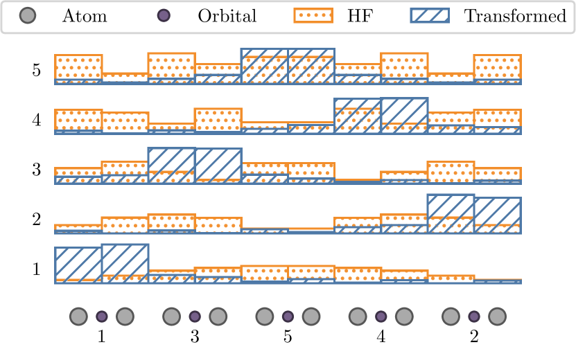
Figure 8: Illustration of our orbital canonicalization. The bottom row illustrates the hydrogen chain with our localized orbitals. Rows 1 to 5 illustrate the contribution of each atom to each of the five orbitals for the Hartree-Fock solution obtained via PySCF (Sun et al., 2018) and our transformed solution. We plot the sum of absolute values of $\Omega$ belonging to atom $i$ as the height of the $i$th bar. Our transformed solution (blue) localizes the contribution close to the nuclei closest to its location.

Algorithm 2 Mask construction

  Input: Atom pairs $(n_{i},m_{i})$, Orbital types $T_{i}\in\mathbb{N}_{+}$, Atomic orbitals $O_{m}$

  # ${\mathbb{P}}$ is a dictionary of dictionaries of lists where the first level is an atom, the second level are orbital types, and the list keeps track of the orbitals.

  Priority ${\mathbb{P}}:=\{\}$

  for $i=1;i\leq N_{\text{orb}}$ do

     ${\mathbb{P}}[n_{i}][T_{i}].\text{append}(i)$

     if $n_{i}\neq m_{i}$ then

        ${\mathbb{P}}[m_{i}][T_{i}].\text{append}(i)$

     end if

  end for

  Offsets $o_{i}:=\sum_{m=1}^{i-1}O_{m}$

  Result ${\bm{M}}:=\bm{0}^{\sum_{m=1}^{M}\times N}$

  # Iterate through all atoms.

  for $n,{\mathbb{T}}_{n}\in{\mathbb{P}}$ do

     # Offset that indicates the lowest free orbital.

     Offset $o:=o_{n}$

     # Iterate through all orbitals types of atom $n$.

     for $T,{\bm{m}}\in{\mathbb{T}}_{n}$ do

        # Iterate through the cardinality orbital type $T$.

        for $i=1;i\leq\dim({\bm{m}})$ do

           ${\bm{M}}_{o+i,m_{i}}:=1$

        end for

        # Since $\dim({\bm{m}})$ many orbitals have been assigned, we must increase the offset.

        $o:=o+\dim({\bm{m}})$

     end for

  end for

  return ${\bm{M}}$

As discussed in Section 4.3, the solution obtained from a Hartree-Fock calculation may not align with our assumptions about the locality of orbitals. Since learning global orbital functions based on our localized orbital embeddings presents a difficult challenge, we seek to canonicalize our Hartree-Fock solutions such that they align with our localized orbitals. As explained in Section 2, in Hartree-Fock one optimizes coefficients of linear combinations of atomic orbital functions to construct molecular orbital functions. Figure 8 shows these coefficients $\Omega^{T}$. Each Hartree-Fock molecular orbital, 1 to 5, exhibits a non-local structure. In the following, we will describe how we transform obtained Hartree-Fock solutions such that they obey a local structure and canonicalize their coefficients to avoid disagreements between similar molecules.

If one considers the HF electronic wave function $\psi({\mathbf{r}})=\det\Phi=\det\varPhi\Omega^{T}$, one can see that the wave function does not change if one multiplies the coefficient matrix $\Omega^{T}$ with a matrix with unit determinant ${\bm{A}}\in\mathbb{R}^{N\times N}$ on the right, i.e., $\psi({\mathbf{r}})=\det\varPhi\Omega^{T}{\bm{A}}$. As the sign of the wave function is arbitrary, ${\bm{A}}$ may also have a determinant of $-1$. Since we know the atoms involved in the localization of the $i$th molecular orbital, we can formulate an optimization problem as

$$\min_{\bm{A}} \|\Omega^{T}{\bm{A}}\circ(1-{\bm{M}})\|^{2}_{2}+\sum_{i=1}^{N}(1-\|(\Omega^{T}{\bm{A}}\circ{\bm{M}})_{i}\|_{2})^{2}$$ (46)

s.t. $$|\det{\bm{A}}|=1$$ (47)

where ${\bm{M}}\in\{0,1\}^{N\times\eta},\eta=\sum_{m=1}^{M}O_{m}$ is a binary mask indicating our desired relation between atomic and molecular orbitals. Note, that the first term in Equation (46) encourages zero interaction with non-involved atoms, and the second term aids in keeping the wave function normalized.

In our matching mask ${\bm{M}}$, we want to preserve the order of energy levels. Atomic orbitals are typically sorted by energy level, i.e., the $i$th orbital has lower energies than the $j$th atomic orbital iff $i<j$. To get a canonical ordering, we translate these energy levels to our localized orbitals. Specifically, we want our localized core orbitals to match the atomic orbitals in the same order, i.e., our $i$th core orbital of an atom should match the $i$th atomic orbital. For valence orbitals, we enforce the same for bonds of higher order (double bonds, triple bonds, …) where we match the first valence orbital of that bond to the lowest free orbitals of both atoms and the second bond to the second lowest free orbitals of both, etc. If an atom has bonds to $k$ different atoms, we cannot easily define an order between bonds and, thus, distribute the $k$ free orbitals of both atoms equally to the $k$ different bonds.

We illustrate this in an example of H₂O. Hydrogen has 1 atomic orbital and oxygen 5 (the number of atomic orbitals is determined by the period of the element), i.e., $\eta=6$. The number of molecular orbitals is $\lceil\frac{\sum_{m=1}^{M}Z_{m}}{2}\rceil=5$. Now, assuming an equilibrium structure, our molecular orbitals are distributed as follows: three core orbitals associated with oxygen and one valence orbital for each of the O-H bonds. Given our mask construction, we get the following mask

$${\bm{M}}_{\text{H2O}} =\left[\begin{array}[]{ccccc|c|c}1&0&0&0&0&0&0\\ 0&1&0&0&0&0&0\\ 0&0&1&0&0&0&0\\ \hline\cr 0&0&0&1&1&1&0\\ 0&0&0&1&1&0&1\\ \end{array}\right]$$ (53)

where the first three rows are core-orbitals and the last two rows are valence-orbitals. The vertical lines group the atomic orbitals by the associated atom, the first five columns belong to the oxygen atom while the last two belong to each of the hydrogen atoms. A formal definition of our mask construction is given in Algorithm 2.

Finally, we solve Equation (46) with an alternating optimization algorithm. In the first step, we optimize ${\bm{A}}$ with the Broyden-Fletcher-Goldfarb-Shannon (BFGS) algorithm (Nocedal & Wright, 2006) where we parametrize $\hat{{\bm{A}}}$ with real numbers but normalize it with ${\bm{A}}=\frac{1}{\sqrt[N]{|\det{\bm{A}}|}}\hat{{\bm{A}}}$ before computing the loss. Because this restriction cannot change the sign of the determinant ${\bm{A}}$ and permutation represent local minima, we use the Hungarian algorithm (Kuhn, 1955) to optimize over all permutations given a fixed ${\bm{A}}$. We compute the cost matrix for the Hungarian algorithm by evaluating the Equation (46) for all possible pairwise permutations. After finding the optimal permutation matrix ${\bm{P}}^{(t)}$, we merge it into ${\bm{A}}^{(t+1)}={\bm{A}}^{(t)}{\bm{P}}^{(t)}$. We either stop after a fixed number of iterations or after the loss does not change. Typically, this method converges within 2 iterations. Since we have to do this only once as preprocessing before pretraining, one can neglect the computational cost, which is in the order of a second per molecule.

As the sign of the wave function is arbitrary, we should decide on a canonical sign for each molecular orbital to avoid mismatches between different Hartree-Fock solutions of similar structures. We implement this by multiplying ${\bm{M}}$ with a diagonal matrix ${\bm{D}}$ where the diagonal elements are defined as

$${\bm{D}}_{ii}=\begin{cases}-1&\text{ if }\sum_{j=1}^{\eta}(\Omega^{T}A\circ{\bm{M}})_{ij}<0,\\ 1&\text{else}.\end{cases}$$ (54)

Appendix E Pretraining regularization

Since we found the output of the reparametrization network to be unstable during pretraining, we add a small regularization to its output. Specifically, we define for each parameter matrix it outputs a target normal distribution, i.e., a mean and variance. For instance, for weight matrices $\bar{{\bm{W}}}\in\mathbb{R}^{d_{\text{in}}\times d_{\text{out}}}$, such the ones in Equation (42) or Equation (19), we follow the standard initialization and define the mean to be zero and the standard deviation to be $\frac{1}{\sqrt{d_{\text{in}}}}$ (LeCun et al., 2012). In our regularization loss, we then enforce that the outputted distribution follows our target normal distribution by matching the first $p_{\text{max}}$ moments of the output distribution with the moments of the target distribution. Concretely, for the $i$th outputted parameters we add the following loss

$$\mathcal{L}_{\text{pre}}(\theta_{i})= \sum_{p=1}^{p_{\text{max}}}\left(\frac{1}{|\hat{\theta}_{i}|}\left(\sum_{j=1}^{|\hat{\theta}_{i}|}\hat{\theta}_{ij}^{p}\right)-m_{p}\right)^{2},$$ (55)

$$\hat{\theta}_{i}= \frac{(\theta_{i}-\mu_{i})}{s_{i}},$$ (56)

$$m_{p}= \begin{cases}0&\text{if }$p$\text{ is odd},\\ (p-1)!!&\text{if }$p$\text{ is even}\end{cases}$$ (57)

where $\theta_{i}$ is $i$th outputted parameter, $\mu_{i}$ is its target mean, $s_{i}$ its target standard deviation, $!!$ the double factorial and $m_{p}$ is the $p$th central moment of a standard normal distribution.

Appendix F Rescaling gradients

In the following, we discuss a gradient rescaling technique on a per-molecule basis to obtain a stable optimization if one optimizes molecules of different sizes jointly. As the norm of gradients in Equation (10) is proportional to the expected deviation from the mean, the standard deviation of the energy functions as a proxy for the gradient's norm. We rescale the gradients based on this proxy rather than the actual gradient norm as acquiring the latter is inherently expensive as it requires one to compute the full Jacobian of the network rather than a Jacobian vector product. Given the standard deviations $s_{i}=\sqrt{\mathbb{E}_{x\sim\psi_{\theta_{i}}^{2}}\left[E_{\theta_{i}}(x)-\mathbb{E}_{x\sim\psi_{\theta_{i}}^{2}}\left[E_{\theta_{i}}(x)\right]\right]^{2}}$ where $\theta_{i}$ indicates the parameters outputted by the reparametrization network for the $i$th molecule. We rescale the gradients of the $i$th molecule with $\min\left(1,\frac{1}{s_{i}}\right)$. This way small gradients are not scaled up but large gradients are scaled down.

Appendix G VMC optimization

A VMC step consists of three substeps: 1) sampling the square of the wave function $\psi_{\theta}^{2}$, 2) Computing the local energy $E_{\theta}({\mathbf{r}})$ and gradients $\nabla_{\theta}E$ and 3) preconditioning the gradient with natural gradient descent ${\bm{F}}^{-1}\nabla_{\theta}E$. To sample the electronic wave function $\psi_{\theta}$, we use Metropolis-Hastings, i.e., in multiple iterations we perturb the electron positions from the last step with gaussian noise and perform rejection sampling based on the square of the wave function $\psi_{\theta}$. Next, we compute the local energies for each electron configuration as in Equation (9) and use these samples to approximate the gradients with Equation (10). Finally, we precondition the gradient with the inverse of the Fisher information matrix (FIM). As the FIM scales quadratically with the number of parameters, realizing it and computing its inverse is infeasible. Instead, we use the conjugate-gradient (CG) method to approximate its inverse (Neuscamman et al., 2012). For efficiency reasons, we compute the output of the reparametrization network once for the first two steps as it's constant throughout sampling and energy calculations. Before applying the update, we clip the norm of the gradient to 1 (Pascanu et al., 2013) such that different system sizes do not require different choices of learning rates (Gao & Günnemann, 2022).

Appendix H Experimental setup

Table 2: Default hyperparameters.

	Hyperparameter	Value
Pretraining	Steps	1e4
	Basis	STO-6G
	Method	RHF
Optimization	Steps	6e4
	Learning rate	$\frac{0.1}{1+\frac{t}{100}}$
	Batch size	4096
	Damping	1e-4 $\sigma[E_{L}]$
	Local energy clipping	5
	Max grad norm	1
	CG max steps	100
MCMC	Target pmove	0.5
	# Steps	40
Moon	Hidden dim	256
	E-E int dim	32
	Layers	4
	Activation	SiLU
	Determinants	16
	Jastrow layers	3
	Filter hidden dims	[16, 8]
Reparametrization	Embedding dim	128
	MLP layers	4
	Message dim	64
	Layers	3
	Activation	SiLU
	Filter hidden dims	[64, 16]

We implemented all experiments and methods in JAX (Bradbury et al., 2018). As we cannot rely on fixed tensor shapes like in previous work where only the spatial arrangements varied within a batch, we implemented everything with masking operations. We generally parallelize all operations where possible over all molecules within a batch. Exceptions are determinant calculations and the computation of the local energy. While one can parallelize the determinant operation if one pads smaller matrices, we found this parallelization to be slower than performing the determinant calculations sequentially. For computing the local energy, one needs to compute the Laplacian, i.e., the trace of the Hessian, of the log wave function. This is a computationally demanding task where higher memory efficiency can be achieved by serializing across molecules and electrons.

For pretraining, we use the LAMB optimizer (You et al., 2020) while for VMC we use gradient descent with a maximal gradient norm of 1. During VMC, we apply the gradient clipping from von Glehn et al. (2023), i.e., we clip all deviations from the median larger than 5 times the mean absolute deviation before computing the mean of the local energies.

All experiments ran on 1 to 4 Nvidia A100 GPUs depending on the system size. If not otherwise specified, we use the hyperparameters from Table 2.

Appendix I Molecular structures

Here, we list for each of our experiments the molecular structures and reference calculations.

For testing training on similar structures, we use the hydrogen rectangle from Pfau et al. (2020). For the six-element hydrogen chain, we use the pretraining geometries from Scherbela et al. (2022), and for the ten-element hydrogen chain, we use the geometries from Motta et al. (2017).

The extended hydrogen chains for the extensivity experiment are generated by having a $n$-element chain of hydrogen atoms with interatomic distances of $1.8\text{\,}\mathrm{a_{0}}$.

For testing dissimilar structures, we use the same distances for nitrogen as in Pfau et al. (2020). As reference energy, we use twice the atomic energy of nitrogen from Chakravorty et al. (1993) plus the experimental dissociation energy from Le Roy et al. (2006). For the additional hydrogen chain, we reuse the geometries from Motta et al. (2017). For ethene, we use the evaluation structures from Scherbela et al. (2022).

In our transferability experiment, we take the six-element and ten-element hydrogen chain as well as the methane, and ethene structures and energies from Scherbela et al. (2022). The cyclobutadiene structures are from Lyakh et al. (2012) with the final VMC energies of Gao & Günnemann (2023) as reference.

For benzene, we reuse the same geometry from Ren et al. (2022) as previous works.

Appendix J Timings

Table 3: Forward pass timings of FermiNet, Moon, and Globe.

(# nuclei / #electrons)	FermiNet	Moon	Globe
1 / 10	$1.8\text{\,}\mathrm{\SIUnitSymbolMicro s}$	$1.6\text{\,}\mathrm{\SIUnitSymbolMicro s}$	$1.1\text{\,}\mathrm{ms}$
1 / 40	$10.1\text{\,}\mathrm{\SIUnitSymbolMicro s}$	$8.2\text{\,}\mathrm{\SIUnitSymbolMicro s}$	$1.2\text{\,}\mathrm{ms}$
1 / 80	$32.0\text{\,}\mathrm{\SIUnitSymbolMicro s}$	$25.5\text{\,}\mathrm{\SIUnitSymbolMicro s}$	$1.4\text{\,}\mathrm{ms}$
10 / 10	$2.2\text{\,}\mathrm{\SIUnitSymbolMicro s}$	$4.5\text{\,}\mathrm{\SIUnitSymbolMicro s}$	$2.3\text{\,}\mathrm{ms}$
10 / 40	$12.1\text{\,}\mathrm{\SIUnitSymbolMicro s}$	$14.7\text{\,}\mathrm{\SIUnitSymbolMicro s}$	$2.5\text{\,}\mathrm{ms}$
10 / 80	$36.7\text{\,}\mathrm{\SIUnitSymbolMicro s}$	$39.0\text{\,}\mathrm{\SIUnitSymbolMicro s}$	$2.6\text{\,}\mathrm{ms}$
20 / 40	$15.2\text{\,}\mathrm{\SIUnitSymbolMicro s}$	$21.7\text{\,}\mathrm{\SIUnitSymbolMicro s}$	$3.1\text{\,}\mathrm{ms}$
20 / 80	$44.3\text{\,}\mathrm{\SIUnitSymbolMicro s}$	$55.6\text{\,}\mathrm{\SIUnitSymbolMicro s}$	$3.1\text{\,}\mathrm{ms}$

Table 3 lists the timings for the forward pass of FermiNet, Moon, and Globe. For systems with few nuclei, we find Moon to perform faster than FermiNet while reaching higher accuracies. Though, this advantage reverses with an increasing number of nuclei due to the focus on electron-nuclei interactions.

While Globe's forward pass is significantly slower than FermiNet's or Moon's it must only be executed once per step, i.e., sampling and energy computations do not require the reparametrization network but just the wave function.

Appendix K Parameters

Table 4: Parameter counts for FermiNet, PsiFormer, Moon, and Globe.

FermiNet	PsiFormer	Moon	Globe
0.7M	1.6M	1M	13M

In Table 4, we list the number of parameters for FermiNet (Pfau et al., 2020), PsiFormer (von Glehn et al., 2023), Moon, and Globe. With its 300k more parameters, we found Moon to outperform FermiNet significantly in various benchmarks. Compared to PsiFormer, we find Moon to perform similarly with 600k fewer parameters.

Globe's large number of parameters is mostly due to the lage output space, e.g., 10M are concentrated in a dense layer to predict the 8192-dimensional output space for the 32 $\tilde{w}_{i}^{k\delta}\in\mathbb{R}^{256}$ orbital embeddings, see Equation 25.

Appendix L Moon size ablation

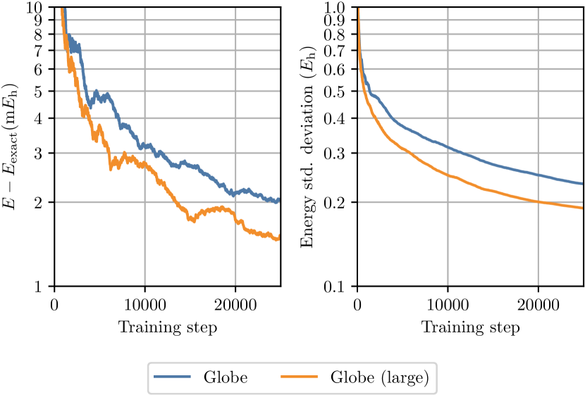
Figure 9: Abalation of Moon where the hidden dimension has been increased to 512 and the number of determinants to 32. In agreement with previous work, we find that increasing the size of the wave function improves variational results accordingly (Spencer et al., 2020; von Glehn et al., 2023).

While jointly training on diverse molecules seems to decrease the accuracy of neural wave functions, here we want to investigate the effect of the size of the network on training. We perform the common augmentation of increasing the hidden dimension to 512 and the number of determinants to 32 (Spencer et al., 2020; von Glehn et al., 2023) and compare the average energy on the diverse small molecule dataset from Section 5.

The energy during training in Figure 9 agrees with previous results on neural network wave functions that increasing the network size increases accuracy (Spencer et al., 2020; von Glehn et al., 2023). As learning diverse molecular wave functions within a single neural network may require more parameters than learning a single wave function, we already see such improvements in small molecules.

Appendix M Standard deviation on hydrogen systems

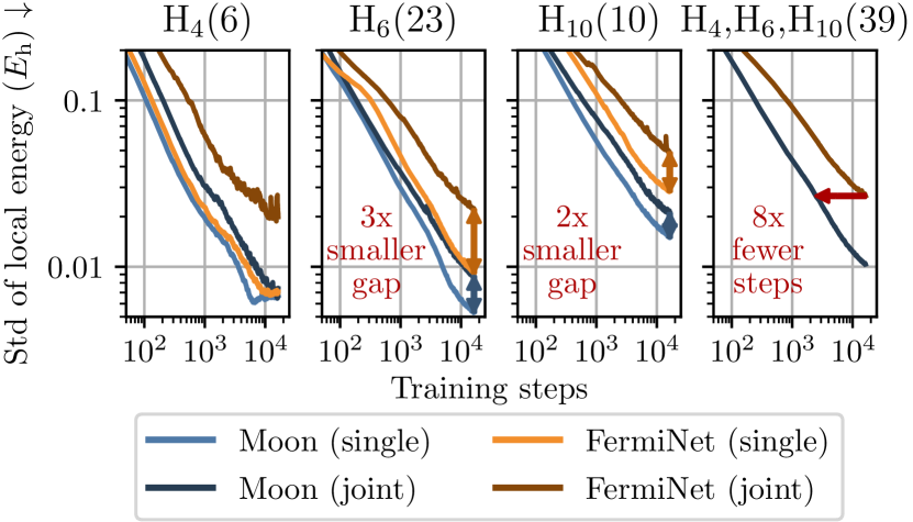
Figure 10: Convergence plots of Globe with Moon and FermiNet. Numbers in brackets show the number of geometries per molecule. In joint training, Moon converges 8 times faster and closes the gap to individual training by a factor of at least 2.

While the energy of a system is a good indicator of convergence, any ground-state wave function will have no standard deviation in its local energy. Thus, we can take a look at the standard deviation of the local energy as a proxy for the convergence of a wave function. In Figure 10, we plot the standard deviation during the training on similar hydrogen systems. We observe that Moon converges 8 times faster in joint training while also closing the gap to the individual trainings by a factor of at least 2.

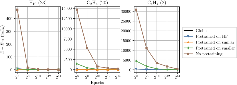
Figure 11: Extended view of Figure 6 without a limit on the y-axis. Convergence of Globe suffers

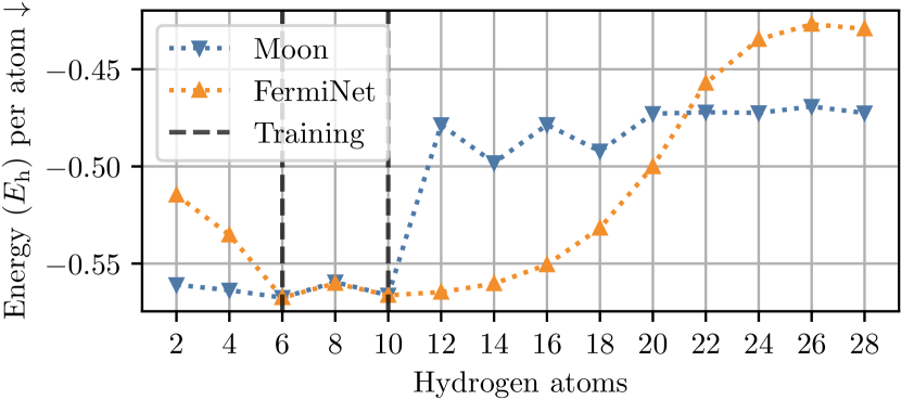
Figure 12: Evaluation of Globe with Moon and FermiNet, trained on small hydrogen clusters, on $n$-elment hydrogen chains. Thanks to Globe's localized orbitals, the energy per atom converges to a constant value for longer chains.

Appendix N Extensivity

We analyze the behavior of Globe with Moon and FermiNet on increasing lengthy hydrogen chains. We first train Globe on the same hydrogen structures as in the previous experiment, i.e., H₄, H₆, and H₁₀. After training, we evaluate Globe on smaller and larger $n$-element hydrogen chains.

Figure 12 depicts the scaling behavior of Moon and FermiNet depending on the system size. As both are upper bounds to the true energy, lower energies are better. Considering that no finetuning is done, neither FermiNet nor Moon diverges far from the trained energies per atom. Interestingly, Moon performs better to smaller substructures like the hydrogen dimer H₂ but results in higher energies for moderately larger chains. Thanks to its locality, Moon's energy per atom is lower than FermiNet's with further increasing system sizes.

Appendix O Extended view on transferibility

As Figure 6 in Section 5 does not include the training curves for ethene and cyclobutadiene without pretraining, we present an extended version in Figure 11. One can see that dropping pretraining impedes convergences. Meanwhile, thanks to its graph-learned approach to molecular orbitals, Globe, with pretraining on smaller molecules, is the first method to reach convergence on larger structures without performing a SCF calculation first.

References

- Ba et al. (2016) Ba, J. L., Kiros, J. R., and Hinton, G. E. Layer Normalization, July 2016.
- Bradbury et al. (2018) Bradbury, J., Frostig, R., Hawkins, P., Johnson, M. J., Leary, C., Maclaurin, D., Necula, G., Paszke, A., VanderPlas, J., Wanderman-Milne, S., and Zhang, Q. JAX: Composable transformations of Python+NumPy programs, 2018.
- Carleo & Troyer (2017) Carleo, G. and Troyer, M. Solving the Quantum Many-Body Problem with Artificial Neural Networks. Science, 355(6325):602–606, February 2017. ISSN 0036-8075, 1095-9203. doi: 10.1126/science.aag2302.
- Cassella et al. (2023) Cassella, G., Sutterud, H., Azadi, S., Drummond, N. D., Pfau, D., Spencer, J. S., and Foulkes, W. M. C. Discovering Quantum Phase Transitions with Fermionic Neural Networks. Physical Review Letters, 130(3):036401, January 2023. doi: 10.1103/PhysRevLett.130.036401.
- Ceperley et al. (1977) Ceperley, D., Chester, G. V., and Kalos, M. H. Monte Carlo simulation of a many-fermion study. Physical Review B, 16(7):3081–3099, October 1977. doi: 10.1103/PhysRevB.16.3081.
- Chakravorty et al. (1993) Chakravorty, S. J., Gwaltney, S. R., Davidson, E. R., Parpia, F. A., and p Fischer, C. F. Ground-state correlation energies for atomic ions with 3 to 18 electrons. Physical Review A, 47(5):3649–3670, May 1993. doi: 10.1103/PhysRevA.47.3649.
- Feynman & Cohen (1956) Feynman, R. P. and Cohen, M. Energy Spectrum of the Excitations in Liquid Helium. Physical Review, 102(5):1189–1204, June 1956. ISSN 0031-899X. doi: 10.1103/PhysRev.102.1189.
- Foulkes et al. (2001) Foulkes, W. M. C., Mitas, L., Needs, R. J., and Rajagopal, G. Quantum Monte Carlo simulations of solids. Reviews of Modern Physics, 73(1):33–83, January 2001. doi: 10.1103/RevModPhys.73.33.
- Gao & Günnemann (2022) Gao, N. and Günnemann, S. Ab-Initio Potential Energy Surfaces by Pairing GNNs with Neural Wave Functions. In International Conference on Learning Representations, April 2022.
- Gao & Günnemann (2023) Gao, N. and Günnemann, S. Sampling-free Inference for Ab-Initio Potential Energy Surface Networks. In The Eleventh International Conference on Learning Representations, February 2023.
- Gasteiger et al. (2021) Gasteiger, J., Becker, F., and Günnemann, S. GemNet: Universal Directional Graph Neural Networks for Molecules. In Advances in Neural Information Processing Systems, May 2021.
- Gerard et al. (2022) Gerard, L., Scherbela, M., Marquetand, P., and Grohs, P. Gold-standard solutions to the Schrödinger equation using deep learning: How much physics do we need? Advances in Neural Information Processing Systems, May 2022.
- Han et al. (2019) Han, J., Zhang, L., and E, W. Solving many-electron Schrödinger equation using deep neural networks. Journal of Computational Physics, 399:108929, December 2019. ISSN 0021-9991. doi: 10.1016/j.jcp.2019.108929.
- Hermann et al. (2020) Hermann, J., Schätzle, Z., and Noé, F. Deep-neural-network solution of the electronic Schrödinger equation. Nature Chemistry, 12(10):891–897, October 2020. ISSN 1755-4330, 1755-4349. doi: 10.1038/s41557-020-0544-y.
- Hermann et al. (2022) Hermann, J., Spencer, J., Choo, K., Mezzacapo, A., Foulkes, W. M. C., Pfau, D., Carleo, G., and Noé, F. Ab-initio quantum chemistry with neural-network wavefunctions, August 2022.
- Hoja et al. (2021) Hoja, J., Medrano Sandonas, L., Ernst, B. G., Vazquez-Mayagoitia, A., DiStasio Jr., R. A., and Tkatchenko, A. QM7-X, a comprehensive dataset of quantum-mechanical properties spanning the chemical space of small organic molecules. Scientific Data, 8:43, February 2021. ISSN 2052-4463. doi: 10.1038/s41597-021-00812-2.
- Jastrow (1955) Jastrow, R. Many-body problem with strong forces. Physical Review, 98(5):1479, 1955.
- Kirkpatrick et al. (2021) Kirkpatrick, J., McMorrow, B., Turban, D. H. P., Gaunt, A. L., Spencer, J. S., Matthews, A. G. D. G., Obika, A., Thiry, L., Fortunato, M., Pfau, D., Castellanos, L. R., Petersen, S., Nelson, A. W. R., Kohli, P., Mori-Sánchez, P., Hassabis, D., and Cohen, A. J. Pushing the frontiers of density functionals by solving the fractional electron problem. Science, 374(6573):1385–1389, December 2021. doi: 10.1126/science.abj6511.
- Kuhn (1955) Kuhn, H. W. The Hungarian method for the assignment problem. Naval research logistics quarterly, 2(1-2):83–97, 1955.
- Le Roy et al. (2006) Le Roy, R. J., Huang, Y., and Jary, C. An accurate analytic potential function for ground-state N2 from a direct-potential-fit analysis of spectroscopic data. The Journal of Chemical Physics, 125(16):164310, October 2006. ISSN 0021-9606, 1089-7690. doi: 10.1063/1.2354502.
- LeCun et al. (2012) LeCun, Y. A., Bottou, L., Orr, G. B., and Müller, K.-R. Efficient backprop. In Neural Networks: Tricks of the Trade, pp. 9–48. Springer, 2012.
- Lennard-Jones (1929) Lennard-Jones, J. E. The electronic structure of some diatomic molecules. Transactions of the Faraday Society, 25(0):668–686, January 1929. ISSN 0014-7672. doi: 10.1039/TF9292500668.
- Li et al. (2022a) Li, X., Fan, C., Ren, W., and Chen, J. Fermionic neural network with effective core potential. Physical Review Research, 4(1):013021, January 2022a. ISSN 2643-1564. doi: 10.1103/PhysRevResearch.4.013021.
- Li et al. (2022b) Li, X., Li, Z., and Chen, J. Ab initio calculation of real solids via neural network ansatz, March 2022b.
- Lyakh et al. (2012) Lyakh, D. I., Musiał, M., Lotrich, V. F., and Bartlett, R. J. Multireference Nature of Chemistry: The Coupled-Cluster View. Chemical Reviews, 112(1):182–243, January 2012. ISSN 0009-2665, 1520-6890. doi: 10.1021/cr2001417.
- Martens & Grosse (2015) Martens, J. and Grosse, R. Optimizing neural networks with Kronecker-factored approximate curvature. In Proceedings of the 32nd International Conference on International Conference on Machine Learning-Volume 37, pp. 2408–2417, 2015.
- Motta et al. (2017) Motta, M., Ceperley, D. M., Chan, G. K.-L., Gomez, J. A., Gull, E., Guo, S., Jiménez-Hoyos, C. A., Lan, T. N., Li, J., Ma, F., Millis, A. J., Prokof'ev, N. V., Ray, U., Scuseria, G. E., Sorella, S., Stoudenmire, E. M., Sun, Q., Tupitsyn, I. S., White, S. R., Zgid, D., Zhang, S., and Simons Collaboration on the Many-Electron Problem. Towards the Solution of the Many-Electron Problem in Real Materials: Equation of State of the Hydrogen Chain with State-of-the-Art Many-Body Methods. Physical Review X, 7(3):031059, September 2017. ISSN 2160-3308. doi: 10.1103/PhysRevX.7.031059.
- Neuscamman et al. (2012) Neuscamman, E., Umrigar, C. J., and Chan, G. K.-L. Optimizing large parameter sets in variational quantum Monte Carlo. Physical Review B, 85(4):045103, January 2012. ISSN 1098-0121, 1550-235X. doi: 10.1103/PhysRevB.85.045103.
- Nocedal & Wright (2006) Nocedal, J. and Wright, S. J. Numerical Optimization 2nd Edition. Springer, 2006.
- Pascanu et al. (2013) Pascanu, R., Mikolov, T., and Bengio, Y. On the difficulty of training recurrent neural networks. In International Conference on Machine Learning, pp. 1310–1318. PMLR, 2013.
- Pfau et al. (2020) Pfau, D., Spencer, J. S., Matthews, A. G. D. G., and Foulkes, W. M. C. Ab initio solution of the many-electron Schrödinger equation with deep neural networks. Physical Review Research, 2(3):033429, September 2020. doi: 10.1103/PhysRevResearch.2.033429.
- Ren et al. (2022) Ren, W., Fu, W., and Chen, J. Towards the ground state of molecules via diffusion Monte Carlo on neural networks, April 2022.
- Scherbela et al. (2022) Scherbela, M., Reisenhofer, R., Gerard, L., Marquetand, P., and Grohs, P. Solving the electronic Schrödinger equation for multiple nuclear geometries with weight-sharing deep neural networks. Nature Computational Science, 2(5):331–341, May 2022. ISSN 2662-8457. doi: 10.1038/s43588-022-00228-x.
- Schütt et al. (2018) Schütt, K. T., Sauceda, H. E., Kindermans, P.-J., Tkatchenko, A., and Müller, K.-R. SchNet – A deep learning architecture for molecules and materials. The Journal of Chemical Physics, 148(24):241722, June 2018. ISSN 0021-9606, 1089-7690. doi: 10.1063/1.5019779.
- Slater (1929) Slater, J. C. The Theory of Complex Spectra. Physical Review, 34(10):1293–1322, November 1929. doi: 10.1103/PhysRev.34.1293.
- Snyder et al. (2012) Snyder, J. C., Rupp, M., Hansen, K., Müller, K.-R., and Burke, K. Finding Density Functionals with Machine Learning. Physical Review Letters, 108(25):253002, June 2012. ISSN 0031-9007, 1079-7114. doi: 10.1103/PhysRevLett.108.253002.
- Spencer et al. (2020) Spencer, J. S., Pfau, D., Botev, A., and Foulkes, W. M. C. Better, Faster Fermionic Neural Networks. 3rd NeurIPS Workshop on Machine Learning and Physical Science, November 2020.
- Sun et al. (2018) Sun, Q., Berkelbach, T. C., Blunt, N. S., Booth, G. H., Guo, S., Li, Z., Liu, J., McClain, J. D., Sayfutyarova, E. R., Sharma, S., Wouters, S., and Chan, G. K.-L. PySCF: The Python-based simulations of chemistry framework. WIREs Computational Molecular Science, 8(1):e1340, 2018. ISSN 1759-0884. doi: 10.1002/wcms.1340.
- Trogolo et al. (2019) Trogolo, D., Arey, J. S., and Tentscher, P. R. Gas-Phase Ozone Reactions with a Structurally Diverse Set of Molecules: Barrier Heights and Reaction Energies Evaluated by Coupled Cluster and Density Functional Theory Calculations. The Journal of Physical Chemistry A, 123(2):517–536, January 2019. ISSN 1089-5639, 1520-5215. doi: 10.1021/acs.jpca.8b10323.
- von Glehn et al. (2023) von Glehn, I., Spencer, J. S., and Pfau, D. A Self-Attention Ansatz for Ab-initio Quantum Chemistry. In The Eleventh International Conference on Learning Representations, February 2023.
- Wilson et al. (2021) Wilson, M., Gao, N., Wudarski, F., Rieffel, E., and Tubman, N. M. Simulations of state-of-the-art fermionic neural network wave functions with diffusion Monte Carlo, March 2021.
- Wilson et al. (2022) Wilson, M., Moroni, S., Holzmann, M., Gao, N., Wudarski, F., Vegge, T., and Bhowmik, A. Wave function Ansatz (but Periodic) Networks and the Homogeneous Electron Gas, February 2022.
- You et al. (2020) You, Y., Li, J., Reddi, S., Hseu, J., Kumar, S., Bhojanapalli, S., Song, X., Demmel, J., Keutzer, K., and Hsieh, C.-J. Large Batch Optimization for Deep Learning: Training BERT in 76 minutes. In Eighth International Conference on Learning Representations, April 2020.
- Zitnick et al. (2022) Zitnick, C. L., Das, A., Kolluru, A., Lan, J., Shuaibi, M., Sriram, A., Ulissi, Z. W., and Wood, B. M. Spherical Channels for Modeling Atomic Interactions. In Advances in Neural Information Processing Systems, October 2022.