Probing the Higgs trilinear self-coupling through Higgs+jet production

Abstract

We present the calculation of the next-to-leading order (NLO) electroweak (EW) corrections proportional to the Higgs trilinear self-coupling ($\lambda_{HHH}$) for Higgs boson plus one jet production at the Large Hadron Collider (LHC). We use the method of large top quark mass expansion to tackle the most challenging two-loop virtual amplitude, and apply the Padé approximation to extend the region of convergence of the expansion. We find that the NLO EW corrections is $0.66\%$ for the total cross section. For the invariant mass distribution and Higgs boson transverse momentum distribution, the NLO corrections are almost flat with their values similar in size. Our results can be used to set extra constraints on $\lambda_{HHH}$ at the LHC.

I Introduction

After the discovery of the Higgs boson 1207.7214; 1207.7235, accurately measuring its properties including various couplings becomes one of the top priorities of the Large Hadron Collider (LHC). The most important reason is that the Higgs boson is related to the spontaneous breaking of electroweak symmetry and is believed to be responsible for the masses of all elementary particles. Also, the Higgs boson may provide the leading portal to possible Hidden sectors beyond the Standard Model (SM). In particular, the Higgs trilinear self-coupling ($\lambda_{HHH}$) is the key parameter in the Higgs potential. The precise determination of its value would give us a better chance to understand electroweak symmetry breaking as well as possible new physics (NP) beyond SM.

The $\lambda_{HHH}$ coupling can be measured directly via the double-Higgs boson production. The very recent observed constraints by direct measurements are $-0.6<\kappa_{\lambda}=\lambda_{HHH}/\lambda_{HHH}^{\rm SM}<6.6$ at $95\%$ confidence level (CL) ATLAS:2022jtk, where $\lambda_{HHH}^{\rm SM}$ is the Higgs trilinear self-coupling in the SM. However, only including the double-Higgs production is not enough to get precise constraints. On the one hand, due to the accidental cancellation between the triangle- and box-type Feynman diagrams at LO in the gluon fusion channel, the total cross section of double Higgs production is heavily suppressed Glover:1987nx; Plehn:1996wb. On the other hand, when using the double-Higgs production to set the constraints, we need strong assumptions on the Higgs coupling modifiers to other SM particles.

Apart from the double-Higgs production processes, $\lambda_{HHH}$ can also appear as loop effects in higher-order electroweak corrections. The observed constraints on $\lambda_{HHH}$ by using the combined single- and double- Higgs production are $-0.4<\kappa_{\lambda}<6.3$ at $95\%$ CL ATLAS:2022jtk, which is better than the constraints from only double-Higgs production. More importantly, using the single-Higgs production allows us to relax the assumptions on the coupling modifiers to other SM particles, e.g. the coupling modifier between the Higgs boson and the top quark ATLAS:2022jtk. In order to investigate this kind of loop effect, the so-called $C$-parameters are introduced in the literature Degrassi:2016wml; Maltoni:2017ims, where different single-Higgs production channels, including VBF, VH, $t\mathrm{bar}{t}H$ and $tHj$ production processes, are analyzed. The authors of Maltoni:2017ims have found that the differential distributions of those single-Higgs production processes can provide extra sensitivity to determine $\lambda_{HHH}$. However, the impacts of differential distributions in the $gg\rightarrow H+j$ process have not been considered in Ref. Maltoni:2017ims because of the highly non-trivial two-loop Feynman integrals.

Recently, a class of two-loop mixed QCD-EW corrections to $gg\rightarrow H+g$ through a loop of light quarks is investigated Bonetti:2020hqh, which doesn’t include the contribution from $\lambda_{HHH}$. In order to include the effect of $\lambda_{HHH}$, we need to consider the contribution from a class of two-loop mixed QCD-EW corrections with a massive top quark loop. The calculation would be quite challenging, due to the appearance of two-loop Feynman integrals with two different internal masses $m_{t}$ and $m_{H}$, and two Mandelstam variables $\hat{s}$ and $\hat{t}$. These integrals are still unknown analytically so far. In this case, approximations can be used to give reliable predictions in certain kinematic regions. For example, the analytic expressions up to $\mathcal{O}[1/(m_{t}^{2})^{3}]$ based on the method of large top quark mass expansion for the two-loop scattering amplitudes of $H\rightarrow ggg$ and $H\rightarrow q\mathrm{bar}{q}g$ are given in Gorbahn:2019lwq, which are used to present the effect of $\kappa_{\lambda}$ corrections on the Higgs boson transverse momentum ($p_{T}$) distribution in DiMicco:2019ngk.

In this work, we focus on the calculation of the $\lambda_{HHH}$ related NLO EW corrections to $pp\rightarrow H+j$ at the LHC and extract the $C$-parameter for the total cross section as well as differential cross sections. We use the method of large top quark mass expansion to tackle the challenging multi-scale two-loop Feynman integrals, which has been proved to be quite reliable for $H+j$ production Chen:2016zka; Chen:2021azt and double-Higgs production below the $2m_{t}$ region Grigo:2015dia; Grazzini:2018bsd. In order to extend the range of validity of the large top quark mass expansion, we adopt the Padé approximation hep-ph/9403230; hep-ph/9605392; hep-ph/0102266; 1605.01380; 1611.05881. This enable us to get reliable predictions in high energy regions, which may be sensitive to NP beyond SM.

This paper is organized as follows. In Sec. II we briefly introduce our notations and present the NLO EW corrections to $pp\rightarrow H+j$ related to $\lambda_{HHH}$ at the LHC. In Sec. III, we show our numerical results and give the $C$-parameter at the levels of total cross section and differential cross sections. The conclusion comes in Sec. LABEL:sec:Conclusion. And we leave the expressions of the form factors to Appendix LABEL:appendix:formfactor.

II Methods

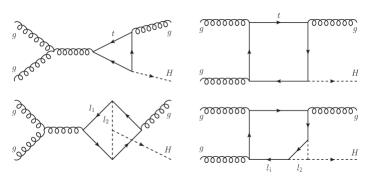
Figure 1: The typical Feynman diagrams for the gluon fusion channel at LO (upper) and NLO (lower) where dashed lines represent the Higgs bosons, solid lines for the top quarks, and curly lines for the gluons. $l_{1}$ and $l_{2}$ are the loop momenta.

We need to consider four partonic processes, $g_{a}(p_{1})+g_{b}(p_{2})\to g_{c}(p_{3})+H(p_{4})$, $q_{a}(p_{1})+\mathrm{bar}{q}_{b}(p_{2})\to g_{c}(p_{3})+H(p_{4})$, $q_{a}(p_{1})+g_{b}(p_{2})\to q_{c}(p_{3})+H(p_{4})$ and $\mathrm{bar}{q}_{a}(p_{1})+g_{b}(p_{2})\to\mathrm{bar}{q}_{c}(p_{3})+H(p_{4})$, where $a,b$ and $c$ are color indices, $q(\mathrm{bar}{q})$ only refer to light (anti-)quark, and $p_{i}$ are the external momenta with $p_{1}^{2}=p_{2}^{2}=p_{3}^{2}=0$ and $p_{4}^{2}=m_{H}^{2}$. We will neglect masses of all light fermions except that of the top quark in our calculation. Take $gg$ channel as an example, therefore at LO, there are only the diagrams including top quark loop. Two typical Feynman diagrams at LO are shown in the upper plots of Fig. 1. At NLO, we only include the diagrams with a top quark loop and the Higgs trilinear self-coupling $\lambda_{HHH}$ vertex. With these considerations, there are 21 Feynman diagrams for the gluon fusion channel at NLO and two of them are showed in the lower plots of Fig. 1.

Before describing the calculation procedures, we first review the definition of the $C$-parameter mentioned in the introduction. Following Ref. Degrassi:2016wml, we consider a beyond SM scenario where the only modification is $\lambda_{HHH}^{\rm SM}$ which can be parameterized via a single parameter $\kappa_{\lambda}$. Therefore, the Lagrangian containing $\lambda_{HHH}^{\rm SM}$ in the Higgs potential after electroweak-symmetry-breaking can be written as $\kappa_{\lambda}\,\lambda_{HHH}^{\rm SM}\,v\,H^{3}$, where $v$ is the vacuum expectation value and $H$ is the physical Higgs field. In presence of the modified trilinear coupling, a generic NLO observable $\Sigma_{\rm NLO}$ (e.g., total or differential cross sections) for single Higgs production can be written as

$$\Sigma_{\rm NLO}=Z_{H}\Sigma_{\rm LO}(1+\kappa_{\lambda}C_{1})\,,$$ (1)

where $Z_{H}$ is the Higgs field renormalization constant, $\Sigma_{\rm LO}$ is the LO observable which is not modified with respect to the SM, and $C_{1}$ is the process- and kinematic-dependent component. Note that the contribution coming from $Z_{H}$ is universal and common to all single-Higgs production processes, whose effect can be considered by introducing $C_{2}$ parameter in Degrassi:2016wml. In this paper, we focus on the process-dependent $C_{1}$ parameter. In the limit $\kappa_{\lambda}\to 1$, $Z_{H}=1+\delta Z_{H}$, and $\Sigma_{\rm NLO}$ goes to its SM value

$$\Sigma_{\rm NLO}^{\rm SM}=\Sigma_{\rm LO}(1+C_{1}+\delta Z_{H})\,,$$ (2)

where we have neglected higher order EW corrections on the right-hand side, and $\delta Z_{H}$ is

$$\delta Z_{H}=-\frac{9}{16\sqrt{2}\pi^{2}}\left(\frac{2\pi}{3\sqrt{3}}-1\right)G_{F}m_{H}^{2}\,,$$ (3)

with $G_{F}$ being the Fermi constant. Therefore, $C_{1}$ can be given by

$$C_{1} =\frac{\Sigma_{\rm NLO}^{\rm SM}-\Sigma_{\rm LO}-\delta Z_{H}\,\Sigma_{\rm LO}}{\Sigma_{\rm LO}}$$

$$=\frac{\sum_{i,j}\int dx_{1}dx_{2}f_{i}(x_{1})f_{j}(x_{2})\,2\Re\left(\mathcal{M}_{\rm LO}^{*}\delta\mathcal{M}_{\rm NLO}^{\rm bare}\right)d\Phi_{2}}{\sum_{i,j}\int dx_{1}dx_{2}f_{i}(x_{1})f_{j}(x_{2})\,|\mathcal{M}_{\rm LO}|^{2}d\Phi_{2}}\,,$$ (4)

where the sum is over all the possible $i$, $j$ partonic initial states of the process, $f_{j}(x_{k})$ is the parton distribution function (PDF) of the parton $j$ with a fraction $x_{k}$ of the initial proton momentum, $d\Phi_{2}$ is the two-body phase-space measure, $\mathcal{M}_{\rm LO}$ is the LO amplitude and $\delta\mathcal{M}_{\rm NLO}^{\rm bare}$ is the NLO amplitude without Higgs field renormalization.

We now turn to the calculation of $\mathcal{M}_{\rm LO}$ and $\delta\mathcal{M}_{\rm NLO}^{\rm bare}$. The amplitudes for the $gg$ and $q\mathrm{bar}{q}$ channels are given by

$$\mathcal{M}^{gg}_{abc} =\sqrt[4]{2}\sqrt{G_{F}}\sqrt{4\pi\alpha_{s}}\,\mathcal{M}_{abc}^{\mu\nu\rho}\epsilon_{\mu}(p_{1})\epsilon_{\nu}(p_{2})\epsilon^{*}_{\rho}(p_{3})\,,$$

$$\mathcal{M}^{q\mathrm{bar}{q}}_{abc} =\sqrt[4]{2}\sqrt{G_{F}}\sqrt{4\pi\alpha_{s}}\,\mathcal{M}_{abc}^{\rho}\,\epsilon^{*}_{\rho}(p_{3})\,,$$ (5)

where $\alpha_{s}$ is the strong coupling constant. Note that the amplitudes $\mathcal{M}^{qg}_{abc}$ for $qg$ channel and $\mathcal{M}^{\mathrm{bar}{q}g}_{abc}$ for $\mathrm{bar}{q}g$ channel can be obtained by applying the crossing symmetry to $\mathcal{M}^{q\mathrm{bar}{q}}_{abc}$. $\mathcal{M}_{abc}^{\mu\nu\rho}$ and $\mathcal{M}_{abc}^{\rho}$ can be written as a linear combinations of independent tensor structures respectively:

$$\mathcal{M}_{abc}^{\mu\nu\rho}= f_{abc}\sum_{i=1}^{4}\mathcal{T}_{gg,i}^{\mu\nu\rho}A_{gg,i}(\hat{s},\hat{t},m_{H},m_{t})\,,$$ (6)

$$\mathcal{M}_{abc}^{\rho}= it_{ab}^{c}\sum_{i=1}^{2}\mathcal{T}_{q\mathrm{bar}{q},i}^{\rho}A_{q\mathrm{bar}{q},i}(\hat{s},\hat{t},m_{H},m_{t})\,,$$ (7)

where the Mandelstam variables are defined as

$$\hat{s}=(p_{1}+p_{2})^{2}\,,\quad\hat{t}=(p_{1}-p_{3})^{2}\,,\quad\hat{u}=(p_{2}-p_{3})^{2}\,,$$ (8)

which satisfy $\hat{s}+\hat{t}+\hat{u}=m_{H}^{2}$. The four tensor structures in Eq. (6) are given by

$$\mathcal{T}^{\mu\nu\rho}_{gg,1} =-\frac{1}{2}\hat{s}p_{1}^{\rho}g^{\mu\nu}+p_{2}^{\mu}p_{1}^{\nu}p_{1}^{\rho}+\frac{\hat{s}\hat{t}p_{2}^{\rho}g^{\mu\nu}}{2\hat{u}}-\frac{\hat{t}p_{2}^{\mu}p_{1}^{\nu}p_{2}^{\rho}}{\hat{u}}\,,$$

$$\mathcal{T}^{\mu\nu\rho}_{gg,2} =\frac{1}{2}\hat{t}p_{1}^{\nu}g^{\mu\rho}+p_{3}^{\mu}p_{1}^{\nu}p_{1}^{\rho}+\frac{\hat{s}\hat{t}p_{3}^{\nu}g^{\mu\rho}}{2\hat{u}}+\frac{\hat{s}p_{3}^{\mu}p_{3}^{\nu}p_{1}^{\rho}}{\hat{u}}\,,$$

$$\mathcal{T}^{\mu\nu\rho}_{gg,3} =\frac{1}{2}\hat{u}p_{2}^{\mu}g^{\nu\rho}+p_{2}^{\mu}p_{3}^{\nu}p_{2}^{\rho}+\frac{\hat{s}p_{3}^{\mu}p_{3}^{\nu}p_{2}^{\rho}}{\hat{t}}+\frac{\hat{s}\hat{u}p_{3}^{\mu}g^{\nu\rho}}{2\hat{t}}\,,$$

$$\mathcal{T}^{\mu\nu\rho}_{gg,4} =-\frac{1}{2}\hat{s}p_{3}^{\mu}g^{\nu\rho}+\frac{1}{2}\hat{s}p_{3}^{\nu}g^{\mu\rho}-\frac{1}{2}\hat{t}p_{2}^{\mu}g^{\nu\rho}+\frac{1}{2}\hat{t}p_{2}^{\rho}g^{\mu\nu}$$

$$+\frac{1}{2}\hat{u}p_{1}^{\nu}g^{\mu\rho}-\frac{1}{2}\hat{u}p_{1}^{\rho}g^{\mu\nu}-p_{2}^{\mu}p_{3}^{\nu}p_{1}^{\rho}+p_{3}^{\mu}p_{1}^{\nu}p_{2}^{\rho}\,.$$ (9)

And the two tensor structures in Eq. (7) are given by

$$\mathcal{T}^{\rho}_{q\mathrm{bar}{q},1} =\left[\frac{\hat{t}}{2}\,\mathrm{bar}{v}(p_{2})\gamma^{\rho}u(p_{1})+\mathrm{bar}{v}(p_{2})\not{p}_{3}u(p_{1})\,p_{1}^{\rho}\right]\,,$$

$$\mathcal{T}^{\rho}_{q\mathrm{bar}{q},2} =\left[\frac{\hat{u}}{2}\,\mathrm{bar}{v}(p_{2})\gamma^{\rho}u(p_{1})+\mathrm{bar}{v}(p_{2})\not{p}_{3}u(p_{1})\,p_{2}^{\rho}\right]\,.$$ (10)

Note that these tensor structures are organized such that the form factors $A_{gg,i}$ and $A_{q\mathrm{bar}{q},i}$ are gauge invariant. To calculate the form factors, we generate the relevant Feynman diagrams using FeynArts Hahn:2000kx. The resulting amplitudes are further manipulated with FeynCalc Mertig:1990an; Shtabovenko:2016sxi; Shtabovenko:2020gxv. Finally, two sets of projection operators constructed from Eq. (9) and Eq. (10) are used to extract $A_{gg,i}$ and $A_{q\mathrm{bar}{q},i}$ from the amplitudes $\mathcal{M}_{abc}^{\mu\nu\rho}$ and $\mathcal{M}_{abc}^{\rho}$ respectively, which can be found in Ref. Gehrmann:2011aa. The form factors can be perturbatively expanded according to

$$A_{gg\,(q\mathrm{bar}{q}),i}=\frac{\alpha_{s}}{4\pi}\left[A_{gg\,(q\mathrm{bar}{q}),i}^{(0)}+\frac{G_{F}}{2\sqrt{2}\pi^{2}}A_{gg\,(q\mathrm{bar}{q}),i}^{(1)}+\mathcal{O}\left(G_{F}^{2}\right)\right]\,,$$ (11)

where $A_{gg\,(q\mathrm{bar}{q}),i}^{(0)}$ are the LO contributions and $A_{gg\,(q\mathrm{bar}{q}),i}^{(1)}$ are the NLO contributions which involve the two-loop Feynman integrals with four independent scales $\hat{s},\hat{t},m^{2}_{t}$ and $m_{H}^{2}$. For $A_{gg\,(q\mathrm{bar}{q}),i}^{(1)}$, we only calculate the contributions coming from the two-loop Feynman diagrams with a $\lambda_{HHH}$ vertex, denoted by $A_{gg\,(q\mathrm{bar}{q}),i}^{(1),\rm bare}$. A straightforward calculation of these two-loop Feynman diagrams is very challenging for two reasons. Firstly, it is very difficult to perform Integration-by-Parts (IBP) reduction for the non-planar integral family. Secondly, the analytic results of relevant master integrals are by far unknown. In order to tackle these challenging calculations, we apply the large top quark mass expansion to $A_{gg\,(q\mathrm{bar}{q}),i}^{(1),\rm bare}$. Based on the method of expansion by regions, the integration domains of loop momenta $(l_{1},l_{2})$ are divided into four regions: hard-hard, hard-soft, soft-hard and soft-soft. According to the definition of $l_{1}$ and $l_{2}$ shown in Fig. 1, only hard-hard and hard-soft regions contribute. Combining the contribution from these two regions, we obtain the final results of the Feynman integrals in the limit $m_{t}^{2}\gg\hat{s},|\hat{t}|,m_{H}^{2}$.

In our work, $A_{gg\,(q\mathrm{bar}{q}),i}^{(1),\rm bare}$ are expanded up to $\mathcal{O}[1/(m_{t}^{2})^{6}]$ (N⁶LP). The most time consuming part is the IBP reduction of huge number of Feynman integrals after expansion by regions. At N⁶LP, there are about 5 million Feynman integrals before IBP reduction. In the large top quark mass limit, the structures of the form factors $A_{gg\,(q\mathrm{bar}{q}),i}^{(1),\rm bare}$ are very simple. Schematically, we present the $\mathcal{O}[1/(m_{t}^{2})^{0}]$ (LP) contributions of the $A_{gg,i}^{(1),\rm bare}$.

$$\vec{A}_{gg}^{(1),\rm bare} =\frac{m_{H}^{2}}{12}\left(-12L_{m}+4\sqrt{3}\pi-23\right)$$

$$\times\left(\frac{1}{\hat{t}},\frac{1}{\hat{s}},-\frac{1}{\hat{s}},\frac{1}{\hat{s}}+\frac{1}{\hat{t}}+\frac{1}{\hat{u}}\right)\,,$$ (12)

where $L_{m}=\ln(m_{t}^{2}/m_{H}^{2})$ and $\sqrt{3}\pi$ terms come from the hard-soft region of the two-loop integrals and $A_{gg,i}^{(1),\rm bare}$ is the $i$-th element of $\vec{A}_{gg}^{(1),\rm bare}$. Note that, there are no ultraviolet (UV) and infrared (IR) divergences in the form factors.

To investigate the validity of large top quark mass expansion, we also expand the LO amplitudes up to $\mathcal{O}[1/(m_{t}^{2})^{12}]$. We will compare the approximate results with the exact results at LO in the next section. For the exact results at LO, we evaluate the one-loop scalar Feynman integrals using program libraries LoopTools Hahn:1998yk and QCDLoop Carrazza:2016gav. We have checked that our LO results are in good agreement with those of MadGraph5_aMC@NLO Alwall:2014hca.

At NLO, the form factors $A_{gg\,(q\mathrm{bar}{q}),i}^{(1),\rm bare}$ have been given up to N³LP in Ref. Gorbahn:2019lwq. It should be noted that the conventions for the form factors are different between Ref. Gorbahn:2019lwq and our work, because of the different choices of tensor structures and normalization factors. After the necessary transformation to arrive at their convention, we find that our results agree with those given in Ref. Gorbahn:2019lwq. For reference, we show the analytic results of $A_{gg\,(q\mathrm{bar}{q}),i}^{(1),\rm bare}$ up to N⁴LP in the Appendix LABEL:appendix:formfactor and give $A_{gg\,(q\mathrm{bar}{q}),i}^{(1),\rm bare}$ up to N⁶LP in an electronic file attached to the arXiv submission, together with $A_{gg\,(q\mathrm{bar}{q}),i}^{(0)}$ up to N¹²LP used in our work.

Note that the approximation in large top quark mass limit is valid only for kinematic region where $\hat{s}<4m_{t}^{2}$. In order to get reliable predictions beyond that region, we adopt the Padé approximation hep-ph/9403230; hep-ph/9605392; hep-ph/0102266; 1605.01380; 1611.05881. Following Ref. hep-ph/9403230, we apply Padé approximation to the expansion series in

$$w\equiv\frac{1-\sqrt{1-s^{\prime}/(4m_{t}^{2})}}{1+\sqrt{1-s^{\prime}/(4m_{t}^{2})}}\,,$$ (13)

instead of in $1/m_{t}^{2}$. Note that $s^{\prime}=\hat{s}$ for $gg$ channel and $q\mathrm{bar}{q}$ channel, and $s^{\prime}=\hat{t}$ for $qg$ channel. With the above knowledge, we can give our numerical predictions for $C_{1}$ parameter defined in Eq. (II).

III Numerical results

In this section we present our numerical predictions for the total cross section, the $m_{jh}$ distribution and the $p_{T}$ distribution, where $m_{jh}=\sqrt{(p_{3}+p_{4})^{2}}$=$\sqrt{\hat{s}}$ is the invariant mass of the Higgs boson and the final state jet, and $p_{T}$ is the transverse momentum of the Higgs boson. We choose the input parameters as $m_{t}=$172.5\text{\,}\mathrm{GeV}$$, $m_{H}=$125.25\text{\,}\mathrm{GeV}$$ and $G_{F}=$$\cite[cite]{\@@bibref{Authors Phrase1YearPhrase2}{ParticleDataGroup:2022pth}{\@@citephrase{(}}{\@@citephrase{)}}}.Ifnotstatedotherwisewechoose$s=$13.6\text{\,}\mathrm{TeV}$$forthehadroniccenter-of-massenergy.OurdefaultPDFsetis\texttt{CT18NNLO\_as\_0118}\cite[cite]{\@@bibref{Authors Phrase1YearPhrase2}{Hou:2019efy}{\@@citephrase{(}}{\@@citephrase{)}}}fortheevaluationofbothLOandNLOcrosssections.Forthestrongcouplingconstantweusethevalueprovidedby\texttt{CT18NNLO\_as\_0118}:$α_s(m_Z)=0.118$.Thedefaultfactorizationscale$μ_f$andrenormalizationscale$μ_r$arechosenas$μ_f=μ_r=(p_T^2+m_H^2+p_T)/2$.Lastbutnotleast,wechoosethecut$p_T ≥$20\text{\,}\mathrm{GeV}$$togetfinitepredictionsforthetotalcrosssectionaswellasthe$m_jh$distribution.\par\begin{figure}[h!]\centering\raisebox{0.0pt}{\includegraphics[width=227.62204pt,height=227.62204pt]{mhj-LO-pp-S.pdf}}\\ \@@toccaption{{\lx@tag[ ]{{2}}{TheLOdifferentialcrosssectionsof$pp\to H+j$withrespecttotheinvariantmass$m_{jh}$oftheHiggsbosonandthejet.ThelowerplotshowstheratiostotheLOexactvalues.}}}\@@caption{{\lx@tag[: ]{{Figure 2}}{TheLOdifferentialcrosssectionsof$pp\to H+j$withrespecttotheinvariantmass$m_{jh}$oftheHiggsbosonandthejet.ThelowerplotshowstheratiostotheLOexactvalues.}}}\@add@centering\end{figure}\par WefirstpresentLOresults.WeshowinFig.~{}\ref{fig:mhj-LO}theLOdifferentialcrosssectionsfor$m_jh$.Inordertoseetheperformanceoflargetopquarkmassexpansionclearly,wepresenttheexactdistributionandthedistributionupto$O[1/(m_t^2)^n]$(N$^n$LP).Theupperplotemploysalogarithmicscalefortheverticalaxistogivethedistributionsinthebroadrange$$140\text{\,}\mathrm{GeV}$ ≤m_jh ≤$2000\text{\,}\mathrm{GeV}$$.ThelowerplotshowstheratiostotheexactvaluesoftheLOdifferentialcrosssection.Asweexpected,thedistributionsintheregion$m_jh≤2m_t$showexcellentconvergenceofthelargetopquarkmassexpansion.TherelativeerrorsofN$^3$LPisalreadysmallerthan$0.3%$.However,thedistributionsatN$^3$LPandN$^6$LPblowupbeyondthetopquarkpairthresholdregion,whichareclearinthelowerplotofFig.~{}\ref{fig:mhj-LO}.Inordertogetreliableestimationsinthe$m_jh≥2m_t$region,weapplythePad\'{e}approximationtotheexpansionseriesin$w$.UsingtheexpansionseriesuptoN$