Controlled nonautonomous matter-wave solitons in spinor Bose-Einstein condensates with spatiotemporal modulation

Abstract

To study controlled evolution of nonautonomous matter-wave solitons in spinor Bose-Einstein condensates with spatiotemporal modulation, we focus on a system of three coupled Gross-Pitaevskii (GP) equations with space-time-dependent external potentials and temporally modulated gain/loss distributions. An integrability condition and a nonisospectral Lax pair for the coupled GP equations are obtained. Using it, we derive an infinite set of dynamical invariants, the first two of which are the mass and momentum. The Darboux transform is used to generate one- and two-soliton solutions. Under the action of different external potentials and gain/loss distributions, various solutions for controlled nonautonomous matter-wave solitons of both ferromagnetic and polar types are obtained, such as self-compressed, snake-like and stepwise solitons, and as well as breathers. In particular, the formation of states resembling rogue waves, under the action of a sign-reversible gain-loss distribution, is demonstrated too. Shape-preserving and changing interactions between two nonautonomous matter-wave solitons and bound states of solitons are addressed too. In this context, spin switching arises in the polar-ferromagnetic interaction. Stability of the nonautonomous matter-wave solitons is verified by means of systematic simulations of their perturbed evolution.

Keywords: Spinor Bose-Einstein condensates; Nonautonomous matter-wave solitons; Darboux transformation; Soliton interactions

I Introduction

For decades, Bose-Einstein condensates (BECs) of ultracold atoms have been studied extensively since their creation in the first experiments [1, 2, 3, 4, 5, 6, 7, 8, 9]. The great interest in this topic has been driven, in particular, by two beneficial features: (1) intrinsic properties of the system, such as the strength of the interatomic interactions, can be manipulated by dint of magnetic fields and lasers; (2) the mean-field theory provides very accurate description of BEC in dilute atomic gases [4, 10, 6, 7, 8, 9].

In particular, broad attention has been attracted to spinor (multi-component) BECs maintained by optical traps [11, 12, 13, 14, 15, 16, 17, 18, 19, 20], as their internal spin degrees of freedom give rise to abundant phenomena, including magnetic crystallization, spin textures and fractional vortices, which have no counterparts in the magnetically trapped condensates with the spin degree being frozen [19, 20, 21]. Many experimental and theoretical studies of spinor BECs have revealed a variety of interesting phenomena, such as polar-to-ferromagnetic phase transitions, quantum knots, condensation of magnon excitations, and various kinds of nonlinear excitations consisting of dark/bright solitons, soliton complexes, rogue waves, vortices, etc. [22, 23]. Matter-wave solitons in atom optics may be used in the design of atom lasers, atom interferometry and coherent atom transport [24, 26, 25]. Matter-wave solitons with internal spin degrees of freedom may find still more diverse application [27, 28]. In the mean-field approximation, the spinor BEC can be described by a set of multicomponent Gross-Pitaevskii (GP) equations [11].

Recently, there has been increased interest in studying spatiotemporally modulated BEC system with time-space-dependent external potentials [29, 30, 31], time-variable gain-loss distribution provided by optical pumping or depletion [32], and time-dependent nonlinearity manipulated by dint of the Feshbach-resonance technique [33, 35, 34, 36]. In particular, the time-dependent terms in the corresponding GP equations can generate various results in the framework of the dynamical management of solitons [37]. The celebrated instances are the dispersion management in fiber optics [37, 38] and nonlinearity management in BEC through the Feshbach resonance technique [33, 34, 35].

In spatiotemporally modulated systems, nonautonomous solitons, which propagate with varying amplitudes and velocities, can be obtained in various physical settings, including hydrodynamics, nonlinear optics, matter waves, etc. [36, 39, 6]. In particular, nonautonomous matter waves in spatiotemporally modulated spinor BECs feature properties different from those of classical matter waves [39, 40, 41, 42].

This paper addresses two aspects. First, we consider integrability conditions for the nonautonomous spin-1 BEC system with a spatiotemporally modulated external potential and time-varying gain-loss distribution, and then derive the respective Lax pair and an infinite set of conservation laws. Second, we construct an $N$-th-order Darboux transformation and study the dynamics of nonautonomous matter-wave solitons of both the ferromagnetic and polar states for the nonautonomous spin-1 BEC system with several different kinds of space-time-dependent external potentials and time-varying gain-loss patterns. Bound states of solitons, and shape-preserving and shape-changing interactions between them are addressed too.

The paper is organized as follows. In Sec. II, the model is formulated for the spinor BEC with the spatiotemporal modulation. In Sec. III, we first derive the integrability condition and nonisospectral Lax pair for the coupled GP equations. Then we derive the infinitely set of conservation laws and put forward the physical meaning of the two lowest-order ones. The $N$-th-order Darboux transform is also derived. In Sec. IV, various controlled nonautonomous matter-wave solitons of both ferromagnetic and polar types are obtained for different external potentials and gain-loss profiles. We also analyze stability of the nonautonomous matter-wave solitons by means of numerical simulations. In Sec. V, shape-preserving and shape-changing interactions between two nonautonomous matter-wave solitons and bound-states of the solitons are addressed. Conclusions are formulated in Sec. VI.

II The model

In the present work, we focus on the dynamics of the spinor BEC with a spatiotemporally-dependent external harmonic-oscillator (HO) potential and time-variable atom gain-loss distributions. Here, we consider the quasi-one dimensional regime: the cigar-shaped trap is elongated in the $x$ direction and strongly confined in the transverse directions $y$ and $z$, which is available to the experiment [43, 44]. In the $F=1$ state, the distribution of atoms is presented by the three-component macroscopic BEC wave function: $\mathbf{\Phi}(x,t)\equiv[\Phi_{+1}(x,t),\Phi_{0}(x,t),\Phi_{-1}(x,t)]$, with the three components pertaining to the three internal states $m_{F}=+1,0,-1$, where $m_{F}$ is the magnetic quantum number. The dynamics of the spinor BEC under the action of spatiotemporally-dependent HO potentials and time-variable gain-loss distributions is governed by the following coupled GP equations within the mean field approximation [11, 45, 17, 18]:

$$\text{i}\hbar\Phi_{\pm 1,t} =-\frac{\hbar^{2}}{2M}\Phi_{\pm 1,xx}+(c_{0}+c_{2})(|\Phi_{\pm 1}|^{2}+|\Phi_{0}|^{2})\Phi_{\pm 1}+(c_{0}-c_{2})|\Phi_{\mp 1}|^{2}\Phi_{\pm 1}+c_{2}\Phi_{0}^{2}\Phi_{\mp 1}^{*}+V_{\text{ext}}(x,t)\Phi_{\pm 1},$$ (1a)

$$\text{i}\hbar\Phi_{0,t} =-\frac{\hbar^{2}}{2M}\Phi_{0,xx}+(c_{0}+c_{2})(|\Phi_{+1}|^{2}+|\Phi_{-1}|^{2})\Phi_{0}+c_{0}|\Phi_{0}|^{2}\Phi_{0}+2c_{2}\Phi_{0}^{*}\Phi_{+1}\Phi_{-1}+V_{\text{ext}}(x,t)\Phi_{0},$$ (1b)

where $V_{\text{ext}}(x,t)$ represents the spatiotemporally modulated external potential and time-dependent gain-loss distribution, $\ast$ stands for the complex conjugate, and $M$ is the atomic mass. Further, $c_{0}=\left(g_{0}+2g_{2}\right)/3$ and $c_{2}=\left(g_{2}-g_{0}\right)/3$ stand, respectively, for the effective constants of the spin-preserving and spin-exchange interaction,

$$g_{f}=\frac{4\hbar^{2}a_{f}}{Ma_{\bot}^{2}(1-Ca_{f}/a_{\bot})}$$ (2)

$(f=0,2)$ denote effective coupling constants, and $a_{f}$ is the $s$-wave scattering length in the channel with the total hyperfine spin $f$. Next, $a_{\bot}$ is the transverse size of the ground state. In the present work, we address the case of $c_{0}=c_{2}=-c<0$, hence $2g_{0}=-g_{2}>0$, which represents the attractive spin-preserving and ferromagnetic spin-exchange interactions. Then, through rescaling $\mathbf{\Phi}\rightarrow(\phi_{+1},\sqrt{2}\phi_{0},\phi_{-1})$ casts system (1) in the form of

$$\text{i}\phi_{\pm 1,t} = -\phi_{\pm 1,xx}-2(|\phi_{\pm 1}|^{2}+2|\phi_{0}|^{2})\phi_{\pm 1}$$ (3a)

$$-2\phi_{0}^{2}\phi_{\mp 1}^{\ast}-v_{\text{ext}}(x,t)\phi_{\pm 1},$$

$$\text{i}\phi_{0,t} = -\phi_{0,xx}-2(|\phi_{+1}|^{2}+|\phi_{0}|^{2}+|\phi_{-1}|^{2})\phi_{0}$$ (3b)

$$-2\phi_{-1}\phi_{0}^{\ast}\phi_{+1}-v_{\text{ext}}(x,t)\phi_{0},$$

where the coordinates and time are, measured, respectively, in units of $$\hbar\sqrt{a_{\bot}/\left(2Mc\right)} \hbar a_{\bot}/c$$ and ,, and

$$v_{\text{ext}}(x,t)\equiv U_{\text{trap}}(x,t)+\text{i}\Gamma(t).$$ (4)

Here

$$U_{\text{trap}}(x,t)=U_{p}(t)x^{2}+\gamma(t)x$$ (5)

is the temporally modulated trapping potential [39, 46], and $\Gamma(t)$ stands for the time-dependent coefficient of the atomic gain and loss, which can be implemented, severally, by loading atoms into the BEC with the optical pump and an electron beam or a strongly focused resonant blast laser in the BEC [47, 48, 49].

III The Lax pair, Darboux transform, and the infinite set of conservation laws

In this section, we aim to derive an integrability condition for system (3) and construct the respective Lax pair and infinite set of dynamical invariants (conservation laws). As system (3) is nonautonomous with the spatiotemporal modulation, to derive the Lax pair, we utilize the generalized Ablowitz-Kaup-Newell-Segur formalism [50] and attempt to construct a nonisospectral Lax pair for system (3) as

$$\Psi_{x}=\mathbf{U}\Psi,~{}~{}\Psi_{t}=\mathbf{V}\Psi$$ (6)

where $\mathbf{U}=\text{i}\lambda(t)J+P$ and $\mathbf{V}=2\text{i}\lambda(t)^{2}J+2\lambda(t)V_{1}+\text{i}V_{0}$, $\lambda(t)$ is a complex nonisospectral parameter,

$$\Psi=(\mathcal{H},\mathcal{Y})^{T}$$ (7)

is the matrix Jost function, $\mathcal{H}$ and $\mathcal{Y}$ are $2\times 2$ matrices, and other matrices are expressed as

$$J =\begin{pmatrix}-I&O\\ O&I\end{pmatrix},~{}~{}P=\begin{pmatrix}O&Q\\ -Q^{{\dagger}}&O\end{pmatrix},$$ (8)

$$V_{0} =\begin{pmatrix}QQ^{{\dagger}}&Q_{x}+2\text{i}\Gamma(t)xQ\\ Q^{{\dagger}}_{x}-2\text{i}\Gamma(t)xQ^{{\dagger}}&-Q^{{\dagger}}Q\end{pmatrix},$$

$$V_{1} =-\text{i}\Lambda(x,t)J+P,~{}\Lambda(x,t)=\left[\Gamma(t)+\frac{\gamma(t)}{4\lambda(t)}\right]x,$$

$$\lambda(t) =\xi e^{-2\int\Gamma(t)\,dt}-\frac{1}{2}e^{-2\int\Gamma(t)\,dt}\int\gamma(t)e^{2\int\Gamma(t)\,dt}\,dt,$$

$$Q =e^{-\frac{\text{i}\Gamma(t)x^{2}}{2}}\begin{pmatrix}\phi_{+1}&\phi_{0}\\ \phi_{0}&\phi_{-1}\end{pmatrix}.$$

Here $I$ and $O$ are the $2\times 2$ unity and zero matrices, “${\dagger}$” stands for the Hermitian conjugate, and $\xi$ is a complex constant. The Lax pair (6) is valid under the following integrability condition imposed on the time-dependent coefficients in potentials (4) and (5):

$$U_{p}(t)=(1/2)\Gamma_{t}(t)+\Gamma^{2}(t),$$ (9)

while $\gamma(t)$ remains an arbitrary real function of $t$. Here, we directly find the integrability condition (9) for the nonautonomous system (3), and then solve the integrable system (3) analytically, by dint of the Darboux transformation. Alternatively, it may be possible to transform the integrable version of the nonautonomous system into the autonomous integrable one discovered in Ref. [45] through an appropriate transformation of $\Phi$ and $x,t$ (as it could be done with many other models [6]), although the latter approach appears to be quite cumbersome for the present system, therefore it is not pursued here.

As mentioned above, in the case of the time-modulated system spectral parameter $\lambda(t)$ is not a constant but a function of $t$, which is determined by coefficients $\Gamma(t)$ and $\gamma(t)$ that, respectively, account for the gain-loss term and linear potential in the system, and complex constant $\xi$. The time-dependent spectral parameter has a significant impact on the nonautonomous matter-wave solitons, which is considered in detail in the following sections.

An important consequence of the integrability of system (3) with Lax pair (6) is that it possesses an infinite set of conservation laws. To derive them, we define an auxiliary matrix function $\Upsilon=\mathcal{H}\mathcal{Y}^{-1}$, in terms of components of the Jost function (7). By substituting $\Upsilon$ it into the Lax pair (6), the following Riccati-type equation can be obtained:

$$\Upsilon_{x}=Q-2\text{i}\lambda(t)\Upsilon+\Upsilon Q^{{\dagger}}\Upsilon,$$ (10)

where $Q$ is given by Eq. (8). Taking the expansion

$$Q^{{\dagger}}\Upsilon=\sum_{k=1}^{\infty}\frac{\Upsilon_{k}}{\lambda(t)^{k}},$$ (11)

where $\Upsilon_{k}$ ($k=1,2,3,\ldots$) are $2\times 2$ matrix functions of $x$ and $t$. Substituting Eq. (11) in Eq. (10) and equating the respective net coefficients in front of each power of $\lambda(t)$ to zero, one derives the following recurrence relations:

$$\Upsilon_{1}= -\frac{\text{i}}{2}Q^{{\dagger}}Q,$$ (12a)

$$\Upsilon_{2}= -\frac{\text{i}}{2}\left[Q_{x}^{{\dagger}}(Q^{{\dagger}})^{-1}\Upsilon_{1}-\Upsilon_{1,x}\right]=\frac{1}{4}Q^{{\dagger}}Q_{x},$$ (12b)

$$\Upsilon_{3}= -\frac{\text{i}}{2}\left[Q_{x}^{{\dagger}}(Q^{{\dagger}})^{-1}\Upsilon_{2}-\Upsilon_{2,x}+\Upsilon_{1}\Upsilon_{1}\right],$$

$$= \frac{\text{i}}{8}(Q^{{\dagger}}Q_{xx}+Q^{{\dagger}}QQ^{{\dagger}}Q),$$ (12c)

$$\vdots$$

$$\Upsilon_{k+1}= -\frac{\text{i}}{2}\left[Q_{x}^{{\dagger}}(Q^{{\dagger}})^{-1}\Upsilon_{k}-\Upsilon_{k,x}+\sum_{j=1}^{k-1}\Upsilon_{j}\Upsilon_{k-j}\right].$$ (12d)

$$(k=2,3,4,\ldots)$$

Then, taking into account the compatibility condition $$(\ln\mathcal{Y})_{xt}=(\ln\mathcal{Y})_{tx}$$, and utilizing Eqs. (11) and (12), we derive the infinite set of conservation laws for system (3) in the form of

$$\frac{\partial U_{j}}{\partial t}=\frac{\partial F_{j}}{\partial x},~{}~{}(j=1,2,3,\ldots)$$ (13)

with

$$U_{1}= ~{}2\text{i}\Upsilon_{1}=Q^{{\dagger}}Q,$$ (14)

$$F_{1}= -2\text{i}\left[-2\Upsilon_{2}+2\Gamma(t)x\Upsilon_{1}+\text{i}Q^{{\dagger}}_{x}(Q^{{\dagger}})^{-1}\Upsilon_{1}\right],$$

$$U_{2}= ~{}4\Upsilon_{2}=Q^{{\dagger}}Q_{x},$$

$$F_{2}= ~{}(-2\text{i})^{2}\left[-2\Upsilon_{3}+2\Gamma(t)x\Upsilon_{2}+\text{i}Q^{{\dagger}}_{x}(Q^{{\dagger}})^{-1}\Upsilon_{2}\right],$$

$$\vdots$$

$$U_{j}= -(-2\text{i})^{j}\Upsilon_{j},$$

$$U_{j}= (-2\text{i})^{j}\left[-2\Upsilon_{j+1}+2\Gamma(t)x\Upsilon_{j}+\text{i}Q^{{\dagger}}_{x}(Q^{{\dagger}})^{-1}\Upsilon_{j}\right],$$

where $U_{j}$ and $F_{j}$ denote the conserved densities and respective fluxes, respectively.

The integrable form of system (3) without the external potential, $v_{\text{ext}}(x,t)=0$, and with constant coefficients has been investigated in Ref. [45], where dynamical invariants were derived. Here, we identify the physical purport of the first few conservation laws obtained here and put forward relations between conservation laws (13) and those derived in Ref. [45] for the integrable system with constant coefficients. According to Eqs. (13), we have the following conserved quantities for system (3):

$$I_{1}= \int dx\,\text{tr}(U_{1})=\int dx\,\text{tr}\{Q^{{\dagger}}Q\},$$ (15a)

$$I_{2}= \int dx\,\text{tr}(U_{2})=\int dx\,\text{tr}\{Q^{{\dagger}}Q_{x}\},$$ (15b)

which are related to the conserved quantities including total number of atoms in the condensate and its total momentum, derived in Ref. [45]:

$$\mathbf{total~{}number:}~{}~{}N_{T}= \int dx\,\mathbf{\Phi^{{\dagger}}}\cdot\mathbf{\Phi}$$

$$= \int dx\,\text{tr}\{Q^{{\dagger}}Q\}=I_{1},$$ (16a)

$$\mathbf{total~{}momentum:}~{}~{}P_{T}= \int dx\,(-\text{i}\hbar\,\mathbf{\Phi^{{\dagger}}}\cdot\partial_{x}\mathbf{\Phi})$$

$$= \int dx\,[-\text{i}\hbar\,\text{tr}\{Q^{{\dagger}}Q_{x}\}]$$

$$= -\text{i}\hbar\,I_{2}$$ (16b)

where “tr” represents the matrix trace. These relations offer the physical identification of the first two dynamical invariants in Eq. (13) as the mass and momentum, respectively. As well as in other integrable systems, the physical interpretation of the higher conserved quantities is not straightforward.

The Darboux transform (DT) is an effective method to construct analytical solutions for the nonlinear evolution equations [51]. We have derived the DT for system (3) based on Lax pair (6) and adopted the obtained DT to construct exact solutions of system (3) for nonautonomous matter-wave solitons. Let $\Psi_{1}=(\mathcal{H}_{1}^{[0]},\mathcal{Y}_{1}^{[0]})^{T}$ be a zero-order complex matrix solution of Lax pair (6) with $Q=Q[0]$ and $\lambda(t)=\lambda_{1}(t)$. Then the DT is used to construct the first-order solution as

$$\Psi[1]= T[1]\Psi,~{}~{}T[1]=\tau_{1}(\lambda)[\lambda I-H[0]\Lambda_{1}H[0]^{-1}],$$ (17a)

$$Q[1]= Q[0]-2\text{i}(\lambda_{1}-\lambda_{1}^{\ast})(\mathcal{Y}_{1}^{[0]}{\mathcal{H}_{1}^{[0]}}^{-1}+\mathcal{H}_{1}^{[0]\ast}{\mathcal{Y}_{1}^{[0]\ast}}^{-1})^{-1},$$ (17b)

with

$$\tau_{1}(\lambda)= [\text{det}(\lambda(t)I-H[0]\Lambda_{1}H[0]^{-1})]^{-\frac{1}{2}}$$ (18)

$$= [(\lambda(t)-\lambda_{1}(t))(\lambda(t)-\lambda_{1}^{*}(t))]^{-\frac{1}{2}},$$

$$H[0]= \begin{pmatrix}\mathcal{H}_{1}^{[0]}&-\mathcal{Y}_{1}^{[0]}\\ \mathcal{Y}_{1}^{[0]}&\mathcal{H}_{1}^{[0]}\end{pmatrix},~{}~{}\Lambda_{1}=\begin{pmatrix}\lambda_{1}(t)I&O\\ O&\lambda_{1}^{*}(t)I\end{pmatrix}.$$

The above results take advantage of the Hermitian-symmetric profile of matrix $Q$ (i.e., $Q^{{\dagger}}=Q^{\ast}$). Making use of this profile, it can be verified that if $\Psi_{1}=(\mathcal{H}_{1}^{[0]},\mathcal{Y}_{1}^{[0]})^{T}$ is a complex matrix solution of Lax pair (6) with $\lambda(t)=\lambda_{1}(t)$, then $\Psi_{1}=(-\mathcal{Y}_{1}^{[0]\ast},\mathcal{H}_{1}^{[0]\ast})^{T}$ is a solution of Lax pair (6) with $\lambda(t)=\lambda_{1}^{\ast}(t)$. The validity of the above DT is established when the following conditions hold: $T[1]_{x}+T[1]U=U[1]T[1]$ and $T[1]_{t}+T[1]V=V[1]T[1]$, where $U[1]$ and $V[1]$ have the same form as $U$ and $V$, except that $Q[0]$ is replaced by $Q[1]$.

In the same way, taking $\Psi_{j}=(\mathcal{H}_{j}^{[0]},\mathcal{Y}_{j}^{[0]})^{T}$ ($j=1,2,3,\ldots$) to be complex matrix solutions of Lax pair (6) with $Q=Q[0]$ and $\lambda(t)=\lambda_{j}(t)$, and iterating the first-order DT $N$ times, we construct the $N$-th-order DT for system (3) as

$$\Psi[N]= T[N]T[N-1]\cdots T[1]\Psi,~{}~{}T[j]=\tau_{j}(\lambda)[\lambda I-H[j-1]\Lambda_{j}H[j-1]^{-1}],$$ (19a)

$$Q[N]= Q[0]-\sum_{j=1}^{N}2\text{i}(\lambda_{j}-\lambda_{j}^{*})\left(\mathcal{Y}_{j}^{[j-1]}{\mathcal{H}_{j}^{[j-1]}}^{-1}+\mathcal{H}_{j}^{[j-1]}{\mathcal{Y}_{j}^{[j-1]}}^{-1}\right)^{-1},$$ (19b)

where

$$\Psi_{j}[j-1]= (\mathcal{H}_{j}^{[j-1]},\mathcal{Y}_{j}^{[j-1]})^{T}$$ (20)

$$= T[j-1]|_{\lambda=\lambda_{j}}T[j-2]|_{\lambda=\lambda_{j-1}}\cdots T[1]|_{\lambda=\lambda_{2}}\Psi_{j},$$

$$\tau_{j}(\lambda)= [(\lambda(t)-\lambda_{j}(t))(\lambda(t)-\lambda_{j}^{*}(t))]^{-\frac{1}{2}},$$

$$H[j-1]= \begin{pmatrix}\mathcal{H}_{j}^{[j-1]}&-\mathcal{Y}_{j}^{[j-1]}\\ \mathcal{Y}_{j}^{[j-1]}&\mathcal{H}_{j}^{[j-1]}\end{pmatrix},\Lambda_{j}=\begin{pmatrix}\lambda_{j}I&O\\ O&\lambda_{j}^{*}I\end{pmatrix}.$$

For the above $N$-th-order DT (19), the following remarks are relevant. (1) As system (3) is nonautonomous with the temporal modulation, the Lax pair (6) is nonisospectral with the time-dependent spectral parameter $\lambda(t)$, which further makes the DT different from that for the spinor BEC system without the external potential, $v_{\text{ext}}(x,t)=0$. (2) $\tau_{j}(\lambda)$ is essential in the DT matrix to make the $t$-part of Lax pair (6) to be satisfied. (3) Because the occurrence of $\tau_{j}(\lambda)$ in the DT matrix, the determinant representation of the above DT (19) can not be expressed directly via Cramer’s rule [52].

IV Nonlinear dynamics of nonautonomous matter-wave solitons with the spatiotemporal modulation

In this section, utilizing the $N$-th-order DT (19) derived in the previous Section, we construct nonautonomous matter-wave-soliton solutions for system (3). To this end, taking the zero seed solution $Q[0]=O$, and substituting $Q[0]$ into Lax pair (6), we derive the matrix Jost function, $\Psi_{1}=(\mathcal{H}_{1}^{[0]},\mathcal{Y}_{1}^{[0]})^{T}$, as

$$\mathcal{H}_{1}^{[0]}=e^{-\theta}I,~{}~{}\mathcal{Y}_{1}^{[0]}=e^{\theta}\Pi^{\ast},$$ (21)

where $\theta=\text{i}\left(\lambda_{1}(t)x+2\int\lambda_{1}^{2}(t)\,dt\right)+\theta_{0}$,

$$\Pi=\begin{pmatrix}a&b\\ b&c\end{pmatrix},$$ (22)

$$\lambda_{1}(t)= \left[\xi_{1}-\frac{1}{2}\int\exp\left(2\int\Gamma(t)\,dt\right)\,\gamma(t)dt\right]\times$$ (23)

$$\exp\left(-2\int\Gamma(t)\,dt\right),$$

$\xi_{1}$, $a$, $b$ and $c$ are complex constants, and $\theta_{0}$ is a real constant which can be used to adjust the initial position of the solitons. We normalize the complex matrix $\Pi$ so that

$$\text{tr}\{\Pi^{{\dagger}}\cdot\Pi\}=|a|^{2}+2|b|^{2}+|c|^{2}=1.$$ (24)

Combining DT (17) and the above matrix Jost function (21), we obtain the one-soliton solutions

$$Q[1]=\frac{4\lambda_{1I}e^{2\theta^{\ast}}}{\Delta}\begin{pmatrix}a+c^{\ast}e^{4\theta_{R}}\text{det}\Pi&b-b^{\ast}e^{4\theta_{R}}\text{det}\Pi\\ b-b^{\ast}e^{4\theta_{R}}\text{det}\Pi&c+a^{\ast}e^{4\theta_{R}}\text{det}\Pi\end{pmatrix}$$ (25)

where

$$\lambda_{1R}= \left[\xi_{1R}-\frac{1}{2}\int\exp\left(2\int\Gamma(t)\,dt\right)\,\gamma(t)dt\right]\times$$ (26)

$$\exp\left(-2\int\Gamma(t)\,dt\right),$$

$$\lambda_{1I}= ~{}\xi_{1I}\exp\left(-2\int\Gamma(t)\,dt\right),$$

$$\theta_{I}= ~{}\lambda_{1R}x+2\int(\lambda_{1R}^{2}-\lambda_{1I}^{2})\,dt,$$

$$\theta_{R}= ~{}\theta_{0}-\left(\lambda_{1I}x+4\int\lambda_{1R}\lambda_{1I}\,dt\right),$$

$$\Delta= ~{}1+e^{4\theta_{R}}+e^{8\theta_{R}}|\text{det}\Pi|^{2},$$

the subscripts $R$ and $I$ representing the real and imaginary parts, respectively. A more compact form of the one-soliton solutions (25) can be written as

$$Q[1]=4\lambda_{1I}\frac{e^{-2\theta_{R}}\left[\Pi+(\sigma_{2}\Pi^{{\dagger}}\sigma_{2})e^{4\theta_{R}}\text{det}\Pi\right]}{e^{-4\theta_{R}}+1+e^{4\theta_{R}}|\text{det}\Pi|^{2}}e^{-2\text{i}\theta_{I}},$$ (27)

where $\sigma_{2}$ is the Pauli matrix. According to the above expressions, we point out the relevance of each parameter for the solitons as follows: $\lambda_{1I}$, the imaginary part of the spectral parameter, is proportional to the amplitude of soliton; its trajectory is determined by $\theta_{R}=0$; and $\Pi$ is the soliton’s polarization matrix. Further, we can conclude that the gain-loss strength $\Gamma(t)$ amplifies or attenuates the soliton’s amplitude, while $\gamma(t)$ has no effect on the amplitude. The trajectory and velocity of the soliton are directly affected by $\Gamma(t)$ and $\gamma(t)$. As for the polarization matrix $\Pi$, it affects spin states of the the soliton. Accordingly, the one-soliton solution may be divided in two types, viz., those for which $\text{det}\Pi$ is zero or not, as first proposed in Ref. [45].

The local spin density of the one-soliton state is

$$\mathbf{f}(x,t)=\mathbf{\Phi^{{\dagger}}}\cdot\mathbf{f}\cdot\mathbf{\Phi}=\text{tr}\{Q^{{\dagger}}\boldsymbol{\sigma}Q\}$$ (28)

[45], where $\mathbf{f}=(f^{x},f^{y},f^{z})^{T}$, with $f^{x,y,z}$ being the $3\times 3$ spin-1 matrices and $\boldsymbol{\sigma}$ the vector of the Pauli matrices. Then, the spin density is derived as

$$\mathbf{f}(x,t)=\frac{16\lambda_{1I}^{2}e^{4\theta_{R}}(1-e^{8\theta_{R}}|\text{det}\Pi|^{2})}{(1+e^{4\theta_{R}}+e^{8\theta_{R}}|\text{det}\Pi|^{2})^{2}}\text{tr}\{\Pi^{{\dagger}}\boldsymbol{\sigma}\Pi\}.$$ (29)

The explicit form for the density of the number of atoms can also be obtained from Eq. (16)

$$n(x,t)=\frac{16\lambda_{1I}^{2}e^{4\theta_{R}}[1+(4e^{4\theta_{R}}+e^{8\theta_{R}})|\text{det}\Pi|^{2}]}{(1+e^{4\theta_{R}}+e^{8\theta_{R}}|\text{det}\Pi|^{2})^{2}}.$$ (30)

The above expressions for the nonautonomous one-soliton solution and its spin and number-of-atoms densities are similar to those for the exact solutions for autonomous solitons derived in Ref. [45]. However, due to the influence of the external potential, characteristics of the nonautonomous solitons for system (3), such as the amplitude, velocity, width, etc., are significantly different from their counterparts in the case of the autonomous solitons. Next, we analyze the dynamics of the nonautonomous solitons under the action of various external potentials.

IV.1 Time-independent external potential and gain-loss distribution

First, we consider the simplest case of the external potential with a constant gain-loss coefficient, $\Gamma(t)\equiv\Omega$, where $\Omega$ is the real constant. In this case, integrability condition (9) determines the time-independent HO potential in Eq. (5) with strength $U_{p}=\Omega^{2}$.

IV.1.1 The nonautonomous ferromagnetic soliton

To separately analyze the influence of the gain-loss coefficient $\Omega$ and linear-potential’s coefficient $\gamma(t)$ (see Eq. (5)) on the dynamics of solitons, we first set $\Omega\neq 0$ and $\gamma(t)=0$. Then the external potential (4) is $v_{\text{ext}}(x,t)=\Omega^{2}x^{2}+\text{i}\Omega$ and we set $\text{det}\Pi=0$. Then, the one-soliton solution (27) reduces

$$Q[1]=2\lambda_{1I}\,\text{sech}(2\theta_{R})e^{-2\text{i}\theta_{I}}\Pi,$$ (31)

where

$$\lambda_{1I}= ~{}\xi_{1I}\,e^{-2\Omega t},~{}~{}\lambda_{1R}=\xi_{1R}\,e^{-2\Omega t},$$ (32)

$$\theta_{I}= ~{}\lambda_{1R}x+2\int(\lambda_{1R}^{2}-\lambda_{1I}^{2})\,dt,$$

$$\theta_{R}= ~{}\theta_{0}-\left(\lambda_{1I}x+4\int\lambda_{1R}\lambda_{1I}\,dt\right).$$

It can be seen that the three components $\{\phi_{+1},\phi_{0},\phi_{-1}\}$ share the same bell-like shape. Solutions (31) yields the amplitude of the soliton as $A=2|\lambda_{1I}|(|a|,|b|,|c|)^{T}$ for the three components $\{\phi_{+1},\phi_{0},\phi_{-1}\}$, velocity $v=-2\xi_{1R}\,e^{-2\Omega t}+2\Omega\theta_{0}\,e^{2\Omega t}/\xi_{1I}$, and the width which is proportional to $e^{2\Omega t}/|\xi_{1I}|$. These results indicate that the amplitude, velocity and width vary with time under the action of the gain-loss term $\sim\Omega$.

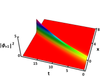
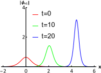
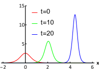
Figure 1: (Top) The 3D plot of the nonautonomous FS soliton of component $\phi_{+1}$. (Middle) The profile of the soliton at different times. (Bottom) The atomic number density $n(x,t)$ at different times. The external potential is $v_{\text{ext}}(x,t)=\Omega^{2}x^{2}+\text{i}\Omega$ and parameters are $\xi_{1}=-0.05+0.8\text{i}$, $\text{det}\Pi=0$, $\Omega=-0.02$, $\theta_{0}=-2$.

The atomic-number density for this solution is $n(x,t)=4\lambda_{1I}^{2}\,\text{sech}^{2}(2\theta_{R})$, and respective total number of atoms is $N_{T}=4\xi_{1I}\,\exp\left(-2\Omega t\right)\equiv N_{T0}\,\exp\left(-2\Omega t\right)$, where $N_{T0}=4\xi_{1I}$ is the initial value of the total number. The spin density of the solution is $\mathbf{f}(x,t)=4\lambda_{1I}^{2}\,\text{sech}^{2}(2\theta_{R})\text{tr}\{\Pi^{{\dagger}}\boldsymbol{\sigma}\Pi\}=n(x,t)\text{tr}\{\Pi^{{\dagger}}\boldsymbol{\sigma}\Pi\}$. Then, the total spin can be calculated as $\mathbf{F}_{T}=4\xi_{1I}\,\exp\left(-2\Omega t\right)\text{tr}\{\Pi^{{\dagger}}\boldsymbol{\sigma}\Pi\}$, and $|\mathbf{F}_{T}|=N_{T}$ for $\text{det}\Pi=0$. Note that the spin density has the same profile as the atomic-number density. With a nonzero total spin, this solution is referred to as the ferromagnetic-state (FS) soliton [45]. As it moves with varying amplitude and velocity, it is also classified as a nonautonomous soliton [39].

In Fig. 1, we show the density profile of the nonautonomous FS soliton for component $\phi_{+1}$ (the other two components $\phi_{0}$ and $\phi_{-1}$ have similar shapes) and the atomic-number density distribution, $n(x,t)$. It is seen that the width of the soliton decreases and its amplitude increases in the course of the evolution at $\Omega<0$ (the case of the gain), as seen in Fig. 1. On the contrary, if $\Omega>0$ (the loss), the width of the soliton increases and amplitude decreases.

IV.1.2 The nonautonomous polar soliton

In this case, we set $\text{det}\Pi\neq 0$ and take the same external potential as above, $v_{\text{ext}}(x,t)=\Omega^{2}x^{2}+\text{i}\Omega$. The expression for the spin density (29) shows that the total spin is always nonzero, i.e., $|\mathbf{F}_{T}|\neq 0$, unless $\Omega=0$ or $2\,|\text{det}\Pi|=1$. Because of the presence of $\lambda_{1I}=\xi_{1I}\,e^{-2\Omega t}$ in spin density (29), which is a time-dependent function, the total spin cannot be zero, which is strongly different from the solution of the integrable spinor BEC system with constant coefficients [45]. There are two special cases that make the total spin to be zero, viz., $\Omega=0$ or $2\,|\text{det}\Pi|=1$. In the case of $\Omega=0$, $\lambda_{1I}$ is time-independent, and a coordinate transformation makes it possible to make the spin density function $\mathbf{f}(x,t)$ an odd function, so the total spin $|\mathbf{F}_{T}|$ is zero. In latter case, the constrain $2\,|\text{det}\Pi|=1$, along with the normalization condition $\text{tr}\{\Pi^{{\dagger}}\cdot\Pi\}=1$, leads to a result $\text{tr}\{\Pi^{{\dagger}}\boldsymbol{\sigma}\Pi\}\equiv(0,0,0)^{T}$. From the expression for the spin density (29), it then follows that the spin density vanishes everywhere, i.e., $\mathbf{f}(x,t)\equiv(0,0,0)^{T}$. Solitons in this state hold the local symmetry of the polar state. Therefore, the solutions given by Eq. (27) with $2\,|\text{det}\Pi|=1$ are referred to the polar-state (PS) solitons, which feature the bell-shaped profile, similar to the FS solitons.

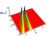
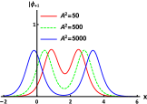
($a$)                                ($b$)

Figure 2: (a) The 3D plot of the nonautonomous PS soliton in component $\phi_{+1}$ with $A^{2}=5000$. (b) The profile of the soliton at $t=0$ with a different polarization matrix $\Pi$. The external potential is $v_{\text{ext}}(x,t)=\Omega^{2}x^{2}+\text{i}\Omega$, and the parameters are $\xi_{1}=-0.05+0.8\text{i}$ and $\Omega=-0.02$.

When polarization matrix is constrained by $2\,|\text{det}\Pi|<1$, the spin density is nonzero. In this case, the single peak of the density split in two for the three components $\{\phi_{+1},\phi_{0},\phi_{-1}\}$, which is different from the FS soliton with $\text{det}\Pi=0$ and PS soliton with $2\,|\text{det}\Pi|=1$. Further, as $|\text{det}\Pi|$ decreases, the twin peaks gradually separate, and behave like two nonautonomous FS solitons. Such solutions are referred to as nonautonomous split solitons. According to solutions (27), three components $\{\phi_{+1},\phi_{0},\phi_{-1}\}$ have similar profiles. In Fig. 2 we display the density profile of the nonautonomous PS soliton in component $\phi_{+1}$ with $A^{2}=5000$, where $A^{-1}=2|\text{det}\Pi|$. As said above, the twin peaks of the PS soliton gradually separate with the increase of $A$, as illustrated in Fig. 2(b). Due to the effect of the gain-loss term, the twin peaks of the split soliton slowly approach, rather than staying parallel, which is different from the case of autonomous integrable system [45]. Parameter $\theta_{0}$ has been used to adjust the positions of the twin peaks with different $A$ in Fig. 2(b).

IV.1.3 Numerical simulations of the evolution of the nonautonomous matter-wave solitons

Next, we use numerical simulations to analyze the stability of the nonautonomous matter-wave solitons. The split-step Fourier method has been applied to analyze the stability in the case of the time-independent external potential, $v_{\text{ext}}=\Omega^{2}x^{2}+\text{i}\Omega$, and constant gain-loss coefficient, $\Gamma(t)\equiv\Omega$. In the simulations, random noise is added to the input taken as the one-soliton solution (27). The stability of the nonautonomous matter-wave solitons is verified for both the ferromagnetic and polar states, as shown in Fig. 3. It is seen that both the FS and PS solitons are indeed dynamically stable in the presence of the random noise.

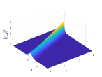
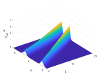
($a$) $A=0$                           ($b$) $A^{2}=5000$

Figure 3: Numerical simulations of the FS and PS solitons. Inputs for the numerical simulations are taken as the one-soliton solution (27) with a random noise level added to it at the $2\%$ level. The other parameters are taken the same as in Figs. 1 and 2.

IV.1.4 Nonautonomous solitons without the gain-loss term

In this case, we set $\Omega=0$ with $\gamma(t)\neq 0$ to analyze the effects of the external potential (4), which reduces to $v_{\text{ext}}(x,t)=\gamma(t)x$. In this condition, the velocity of the soliton is $v=2\int\gamma(t)\,dt-4\xi_{1R}$, its width is inversely proportional to $|\xi_{1I}|$, and the amplitude of the soliton is $A=2|\xi_{1I}|(|a|,|b|,|c|)^{T}$ for the three components $\{\phi_{+1},\phi_{0},\phi_{-1}\}$.

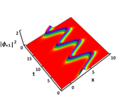
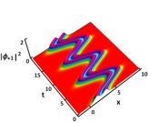
($a$)                                           ($b$)

Figure 4: (a) The 3D plot of the nonautonomous FS soliton in component $\phi_{+1}$ with $A=0$. (b) The 3D plot of the nonautonomous split soliton in component $\phi_{+1}$ with $A^{2}=50$. The external potential is $v_{\text{ext}}(x,t)=(\cos t)x$ and the parameters are $\xi_{1}=0.8\text{i}$ and $\theta_{0}=4$.

It is seen that $\gamma(t)$ has no effect on the amplitude of the soliton, but notably affect the velocity of the soliton. In Fig. 4, by choosing a $\gamma(t)=\cos(t)$, snakelike FS and PS solitons are obtained with a constant amplitude and periodically varying velocity.

As the gain-loss term is absent, the total number of atoms $N_{T}=4\xi_{1I}=N_{T0}$ remains constant, whether $\text{det}\Pi=0$ or not, i.e., the total number of atoms in system (3) is conserved even in the presence of the time-dependent coefficient $\gamma(t)$ in the linear potential. As for the spin density and total spin, it is found that $|\mathbf{F}_{T}|=N_{T}$ for $\text{det}\Pi=0$. When $2|\text{det}\Pi|=1$, spin density $\mathbf{f}(x,t)$ vanishes everywhere and, naturally, the total spin vanishes too, $|\mathbf{F}_{T}|=0$. On the other hand, for $2|\text{det}\Pi|<1$ the spin density $\mathbf{f}(x,t)$ remains nonzero, even though the total spin is again zero, $|\mathbf{F}_{T}|=0$.

IV.2 The time-dependent external potential and gain-loss distribution

Next, we consider the case when the HO potential $U_{p}(t)$ in Eq. (5) is time-dependent and can be attractive or expulsive (inverted HO). Various potential functions $U_{p}(t)$ and gain-loss coefficients $\Gamma(t)$ can be used to generate different nonautonomous matter-wave solitons. We here choose certain physically relevant forms of the external potential to investigate the evolution of several kinds of nonautonomous solitons. In this case, we set $\gamma(t)=0$ in Eq. (5).

IV.2.1 Nonautonomous solitons with a step-wise time-modulated gain-loss coefficient

To amplify a soliton with a small amplitude into one with an appropriate amplitude, the following step-wise gain-loss coefficient can be used:

$$\Gamma(t)=\rho[1+\tanh(2\rho t)],$$ (33)

where $\rho$ determined the steepness of the step and $\delta$ is the initial phase of the step. Then, according to the integrability condition (9), the time-dependent external potential $U_{p}(t)$ (5) is

$$U_{p}(t)\equiv\frac{1}{2}\Omega^{2}(t)=2\rho^{2}[1+\tanh(2\rho t)].$$ (34)

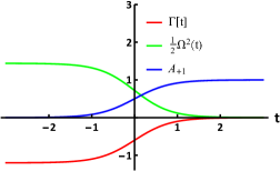
Figure 5: The kink-like shape of the gain-loss coefficient $\Gamma(t)$ (the red line), HO potential strength $(1/2)\Omega^{2}(t)$ (the green line), and amplitude $A_{+1}$ for component $\phi_{+1}$ (the blue line). The parameters are $\rho=-0.6$, $\delta=0$, $a=0.5$ and $\xi_{1I}=-0.5$.

In this case, solution (27), yields the amplitude of the nonautonomous soliton for the three components, $A=2|\lambda_{1I}|(|a|,|b|,|c|)^{T}$ where

$$\lambda_{1I}=\xi_{1I}\,\exp\left(-2\int\Gamma(t)\,dt\right)=\xi_{1I}\,e^{\delta}[1-\tanh(2\rho t)].$$ (35)

In Fig. 5, we show the kink-like shape of the gain-loss coefficient $\Gamma(t)$, HO potential strength $(1/2)\Omega^{2}(t)$, and amplitude $A_{+1}$ of component $\phi_{+1}$. Obviously, $\rho<0$ and $\rho>0$ in Eq. (33) correspond to $\Gamma(t)\leq 0$ and $\Gamma(t)\geq 0$ (the gain and loss), respectively. Accordingly, the parabolic potential and amplitude of the soliton are always non-negative, with the former and latter step-wise decreasing to zero or increasing from zero to a finite value, respectively.

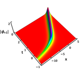
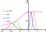
($a_{1}$)                                           ($a_{2}$)
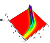
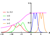
  ($b_{1}$)                                           ($b_{2}$)

Figure 6: Density profiles of ($a_{1}$) the nonautonomous FS soliton with $A=0$ and ($b_{1}$) nonautonomous split soliton with $A^{2}=50$ in component $\phi_{+1}$. ($a_{2}$) and ($b_{2}$) are soliton profiles at different times and peak values (the magenta line) of the soliton fields. The parameters are $\rho=-0.5$, $\delta=0$, $\xi=-0.4-0.5\text{i, }$and $\theta_{0}=5$.

Density profiles of the two kinds of nonautonomous solitons, FS and PS ones, are displayed in Fig. 6. Under the step-wise gain effect ($\Gamma(t)<0$), the nonautonomous solitons are amplified into states with finite constant amplitudes both for the FS and PS solitons. Unlike the previous solitons whose amplitudes increase exponentially with time, the amplitudes of these solitons in Fig. 6 grow to a finite value and remain unchanged, as shown by the magenta curves in Figs. 6($a_{2}$) and ($b_{2}$). To explain this, we find from Eqs. (33), (35) and Fig. 5 that, when the amplitude of the soliton attains the maximum, the gain coefficient $\Gamma(t)$ falls to zero. Furthermore, we find that the PS soliton is asymmetric at the amplitude amplification stage, but when the amplitude reaches the maximum, the double-hump soliton becomes symmetric.

In this case, we find the atom-number density $n(x,t)=4\lambda_{1I}^{2}\text{sech}^{2}(2\theta_{R})$ and total number of atoms $N_{T}=4\xi_{1I}e^{\delta}[1-\tanh(2\rho t)]$ when $\text{det}\Pi=0$, where $\lambda_{1I}$ is given by Eq. (35). It is found that the time dependence of the total number of atoms $N_{T}$ is also kink-like, similar to the amplitude of soliton shown in Fig. 5. When $2|\text{det}\Pi|=1$, the number density is derived as $n(x,t)=8\lambda_{1I}^{2}$sech${}^{2}(2\theta_{R}-(1/2)\ln 2)$, and the total number of atoms is $N_{T}=8\xi_{1I}e^{\delta}[1-\tanh(2\rho t)]$, which is two times larger than in the case of $\text{det}\Pi=0$. As for the spin density and total spin under the condition $\text{det}\Pi=0$, it is found that the spin density is $\mathbf{f}(x,t)=4\lambda_{1I}^{2}\text{sech}^{2}(2\theta_{R})\text{tr}\{\Pi^{{\dagger}}\boldsymbol{\sigma}\Pi\}$, and the total spin is $\mathbf{F}_{T}=4\xi_{1I}e^{\delta}[1-\tanh(2\rho t)]\text{tr}\{\Pi^{{\dagger}}\boldsymbol{\sigma}\Pi\}$ with $|\mathbf{F}_{T}|=4\xi_{1I}e^{\delta}[1-\tanh(2\rho t)]$. We point out that both the total number of atoms and total spin exhibit the same kink-like shape time dependence as the amplitude of the soliton. When $2|\text{det}\Pi|=1$, we find that the spin density vanishes everywhere, i.e., $\mathbf{f}(x,t)\equiv(0,0,0)^{T}$, which is a characteristic of the polar state. When the polarization matrix is constrained by $2|\text{det}\Pi|<1$, the spin density $\mathbf{f}(x,t)$ is not zero but the total spin vanishes, $|\mathbf{F}_{T}|=0$, as shown by the direct calculation.

IV.2.2 Nonautonomous solitons with a double-modulated periodic potential

Above, we have analyzed the effects of the periodic modulation of the coefficient $\gamma(t)$ in front of the linear potential in Eq. (5) on the soliton speed. Here we modulate the amplitude of the soliton by applying the time-periodic modulation to the gain-loss coefficient $\Gamma(t)$ and HO-potential strength $U_{p}(t)$. Namely, we set $\gamma(t)=0$ and

$$\Gamma(t)=\Omega_{0}\sin(\omega t),$$ (36)

where $\Omega_{0}$ and $\omega$ are the intensity and frequency of the periodic modulation. Then, according to the integrability condition (9), we obtain the following double-harmonic modulation format,

$$U_{p}(t)\equiv\frac{1}{2}\Omega^{2}(t)=\frac{1}{2}\Omega_{0}\{\Omega_{0}[1-\cos(2\omega t)]+\omega\cos(\omega t)\}.$$ (37)

Under the action of this modulation, the amplitude of the nonautonomous soliton is $A=2|\lambda_{1I}|(|a|,|b|,|c|)^{T}$ for the three components, where

$$\lambda_{1I}=\xi_{1I}\,\exp\left(-2\int\Gamma(t)\,dt\right)=\xi_{1I}\,\exp\left(2\frac{\Omega_{0}}{\omega}\cos(\omega t)\right).$$ (38)

In Eqs. (36)-(38), the gain-loss coefficient $\Gamma(t)$ periodically varies between $-\Omega_{0}$ to $+\Omega_{0}$ with period $2\pi/\omega$, while $U_{p}(t)$ attains the minimum $-\omega\Omega_{0}/2$ at $t=(2k+1)\pi/\omega$ and maximum $\left(\omega/4\right)^{2}+\Omega_{0}^{2}$ at $t=\left[\arctan\left(\omega/\Omega_{0},\pm\sqrt{16\Omega_{0}^{2}-\omega^{2}}/\Omega_{0}\right)+2k\pi\right]/\omega$, where $k$ is an integer. The fluctuation range of the amplitude of the nonautonomous soliton is $2\xi_{1I}|a|\left[\exp\left(-2\Omega_{0}/\omega\right),\exp\left(-2\Omega_{0}/\omega\right)\right]$ for component $\phi_{+1}$, with period $2\pi/\omega$. We display the gain-loss coefficient $\Gamma(t)$, HO-potential strength $(1/2)\Omega^{2}(t)$, and amplitude $A_{+1}$ in Fig. 7. It is seen that the $\Gamma(t)$ and $(1/2)\Omega^{2}(t)$ perform sign-changing oscillations. We also show the periodic sign-changing oscillations of the trapping HO potential, $U_{\text{trap}}(x,t)=(1/2)\Omega^{2}(t)x^{2}$ in Fig. 8. Nonautonomous solitons, including the FS and PS, ones are stably maintained by the attractive-expulsive sign-changing potential $U_{\text{trap}}(x,t)$, cf. a similar result recently reported for 2D solitons in Ref. [53].

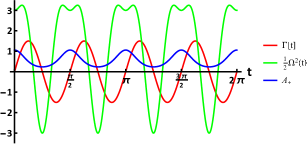
Figure 7: The periodically modulated gain-loss coefficient $\Gamma(t)$ (the red line), HO-potential strength$\ (1/2)\Omega^{2}(t)$ (the green line) and amplitude $A_{+1}$ for component $\phi_{+1}$ (the blue line). The parameters are $\omega=4$, $\Omega_{0}=1.5$, $a=0.5$, and $\xi_{1I}=0.5$.

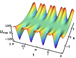
Figure 8: Periodic sign-changing oscillations of the trapping HO potential $U_{\text{trap}}(x,t)=(1/2)\Omega^{2}(t)x^{2}$, cf. a similar time-modulated potential which may maintain stable 2D solitons [53]. The parameters are $\omega=4$ and $\Omega_{0}=1.5$.

Two kinds of breather solitons supported by the periodic modulation of the potential are shown in Fig. 9. Analysis of effects of frequency $\omega$ and scaled amplitude $\Omega_{0}/\omega$ of the modulation (see Eqs. (36) and (37) demonstrates that the breathing amplitude is proportion to $\Omega_{0}/\omega$, as shown in Fig. 9($a_{2}$). Similarly, when $A\neq 0$, i.e., the polarization matrix has $\text{det}\Pi\neq 0$, the PS solitons are obtained, as shown in Figs. 9($b_{1}$) and ($b_{2}$). The twin peaks of the PS soliton gradually separate with the increase of $A$.

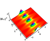
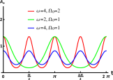
($a_{1}$) $A=0$                                ($a_{2}$)
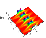
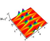
  ($b_{1}$) $A^{2}=50$                      ($b_{2}$) $A^{2}=1000$

Figure 9: Density profiles of ($a_{1}$) the nonautonomous FS soliton with $\theta_{0}=0$, and ($b_{1}$) nonautonomous PS soliton with $\theta_{0}=0.6$ in component $\phi_{+1}$. ($a_{2}$) The effect of frequency $\omega$ and ratio $\Omega_{0}/\omega$ on the breathing dynamics. ($b_{2}$) Nonautonomous PS soliton with $\theta_{0}=1$. The parameters are $\omega=4$, $\Omega_{0}=1.5$ and $\xi_{1}=0.5\text{i}$.

In this case, the number density is $n(x,t)=4\lambda_{1I}^{2}\text{sech}^{2}(2\theta_{R})$ and the total number of atoms is $N_{T}=4\xi_{1I}\,\exp\left(2\left(\Omega_{0}/\omega\right)\cos(\omega t)\right)$ when $\text{det}\Pi=0$, where $\lambda_{1I}$ is given in Eq. (38). The total number of atoms $N_{T}$ and soliton’s amplitude are periodic functions of time with period $2\pi/\omega$, as seen in Fig. 9. When $2|\text{det}\Pi|=1$, the number density is $n(x,t)=8\lambda_{1I}^{2}\text{sech}^{2}(2\theta_{R}-\frac{\ln 2}{2})$ and the total number of atoms is $N_{T}=8\xi_{1I}\,\exp\left(2\left(\Omega_{0}/\omega\right)\cos(\omega t)\right)$, which is twice as large as in the case of $\text{det}\Pi=0$. In the same case, the spin density is $\mathbf{f}(x,t)=4\lambda_{1I}^{2}\text{sech}^{2}(2\theta_{R})\text{tr}\{\Pi^{{\dagger}}\boldsymbol{\sigma}\Pi\}$, and the total spin $\mathbf{F}_{T}=4\xi_{1I}\,\exp\left(2\left(\Omega_{0}/\omega\right)\cos(\omega t)\right)\text{tr}\{\Pi^{{\dagger}}\boldsymbol{\sigma}\Pi\}$ with $|\mathbf{F}_{T}|=4\xi_{1I}\,\exp\left(2\left(\Omega_{0}/\omega\right)\cos(\omega t)\right)$. It is seen that the total number of atoms $N_{T}$ and total spin $|\mathbf{F}_{T}|$ exhibit the same periodic periodic time dependence as the soliton’s amplitude. When $2|\text{det}\Pi|=1$, the spin density vanishes everywhere, i.e., $\mathbf{f}(x,t)\equiv(0,0,0)^{T}$, as it should be in the polar state. When the polarization matrix is constrained by $2|\text{det}\Pi|<1$, the spin density $n(x,t)$ is not zero but the total spin still vanished, $\mathbf{F}_{T}\equiv(0,0,0)^{T}$, as shown by the direct calculation.

IV.2.3 Nonautonomous solitons under the action of sign-reversible gain-loss distribution

Considering the evolution of the solitons under the action of the time-dependent gain-loss term, it is natural to address the case when the gain and loss are globally balanced, so that the respective coefficient $\Gamma(t)$ in Eq. (4) is a localized odd function of time, $\Gamma(-t)=-\Gamma(t)$. The explore this option, we adopt

$$\Gamma(t)=W_{0}\mathrm{sech}(\kappa t)\tanh(\kappa t),$$ (39)

where $W_{0}$ is a real constant and $\kappa>0$ is the temporal-modulation parameter. This form of variable coefficient $\Gamma(t)$ resembles the $\mathcal{PT}$ symmetry [54], but “rotated” in the $\left(x,t\right)$ plane. According to Eq. (9), the respective time-dependent attractive/expulsive HO-potential strength in the integrable system is

$$U_{p}(t) \equiv \frac{1}{2}\Omega^{2}(t)=\frac{1}{2}W_{0}\mathrm{sech}(\kappa t)\{k\,\mathrm{sech}^{2}(\kappa t)$$ (40)

$$-[\kappa-2W_{0}\mathrm{sech}(\kappa t)]\tanh^{2}(\kappa t)\}.$$

In this case, we obtain amplitudes of the three components of the nonautonomous soliton as $A=2|\lambda_{1I}|(|a|,|b|,|c|)^{T}$, where

$$\lambda_{1I}= \,\xi_{1I}\,\exp\left(-2\int_{0}^{t}\Gamma(t^{\prime})\,dt^{\prime}\right)$$ (41)

$$\equiv \,\xi_{1I}\,\exp\left[2\left(W_{0}/\kappa\right)\text{sech}(\kappa t)\right].$$

According to Eq. (39), the gain-loss coefficient $\Gamma(t)$ varies from $-|W_{0}|/2$ to $+|W_{0}|/2$, attaining these values at $t=\mp\mathrm{\ln}\left(\sqrt{2}+1\right)/\kappa$, depending on the sign of $W_{0}$, as shown by red curves in Fig. 10. In this solution, the soliton’s amplitude first grows to $2|\xi_{1I}\,a|\exp\left(2W_{0}/\kappa\right)$ and then returns to the initial value, $2|\xi_{1I}\,a|$, when $W_{0}>0$, or it first decreases to $2|\xi_{1I}\,a|\exp\left(2W_{0}/\kappa\right)$ and then returns to the same initial value, $2|\xi_{1I}\,a|$, when $W_{0}<0$, as shown by blue curves in Fig. 10. Since the total gain-loss distribution $\int\Gamma(t)\,dt=0$. In either case, the soliton recovers to its initial value due to the balance condition, $\int_{-\infty}^{+\infty}\Gamma(t)dt=0$.

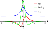
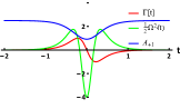
($a$) $W_{0}=2$                                ($b$) $W_{0}=-2$

Figure 10: The sign-reversible gain-loss coefficient $\Gamma(t)$ given by Eq. (39) (the red lines), strength of the HO potential given by Eq. (40) (the green lines) and amplitude $A_{+1}$ for component $\phi_{+1}$ (the blue lines), with $W_{0}>0$ and $W_{0}<0$ in $(a)$ and $(b)$, respectively. Other parameters are $\kappa=4$, $a=0.5$, $\xi_{1I}=1$ for $(a)$ and $\xi_{1I}=2.5$ for $(b)$.

The evolution of the exact soliton solution produced by the present setting is displayed by Fig. 11, for $W_{0}>0$. It is seen from this figure and Eq. (41) that the temporal-modulation parameter $\kappa$ affects the steepness of the arising modulated state and its scaled amplitude, $W_{0}/\kappa$. These states are similar to rogue waves which have been widely studied in nonlinear optics, BEC and fluid mechanics [55]. In particular, the PS soliton is obtained if the polarization matrix is restricted to $2|\text{det}\Pi|\leq 1$, as shown in Figs. 11($b_{1}$) and ($b_{2}$). Note that the single-peak states shown in Figs. 11($a_{1}$) and ($a_{2}$) splits into double-peak ones with the increase of $A$.

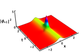
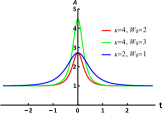
($a_{1}$) $A=0$                                ($a_{2}$)
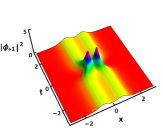
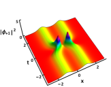
  ($b_{1}$) $A^{2}=50$                      ($b_{2}$) $A^{2}=1000$

Figure 11: Density profiles of the exact solutions corresponding to Eqs. (39) and (40). ($a_{1}$) The nonautonomous FS soliton with $\theta_{0}=0$. ($b_{1}$) and ($b_{2}$): Nonautonomous double-peak solitons with $\theta_{0}=0.6$ and $\theta_{0}=1$, respectively. ($a_{2}$) Effects of the modulation parameter $\kappa$ and amplitude $W_{0}$ on the steepness and amplitude of the solitons. Other parameters are $\kappa=4$, $W_{0}=1.5$ [except for panel ($a_{2}$)], and $\xi_{1}=\text{i}$.

In the case of $W_{0}<0$ in Eq. (39), the exact solution produces, instead of the single- and double-peak states in Fig. 11, ones with dips, as shown, for the solutions of both the FS and PS types, as shown in Fig. 12.

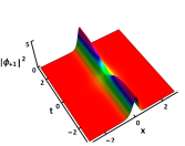
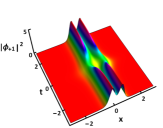
($a$) $A=0$                                ($b$) $A^{2}=50$

Figure 12: Density profiles of solutions of the FS and PS types corresponding to Eqs. (39) and (40). The parameters are $\kappa=2$, $W_{0}=-0.5$, and $\xi_{1}=2\text{i}$.

In this case, we can derive the number density $n(x,t)=4\lambda_{1I}^{2}\text{sech}^{2}(2\theta_{R})$ and the respective total number of atoms $N_{T}=4\xi_{1I}\exp\left[2(W_{0}/\kappa)\mathrm{sech}(\kappa t)\right]$ when $\text{det}\Pi=0$, where $\lambda_{1I}$ is given by Eq. (41). For $2|\text{det}\Pi|=1$, the atomic-number density is $n(x,t)=8\lambda_{1I}^{2}$sech${}^{2}\left[2\theta_{R}-(/2)\ln 2\right]$, and the total number of atoms is $N_{T}=8\xi_{1I}\,\exp\left[2(W_{0}/\kappa)\mathrm{sech}(\kappa t)\right]$, which is twice that in the case of $\text{det}\Pi=0$. The spin density of this solution is $\mathbf{f}(x,t)=4\lambda_{1I}^{2}\text{sech}^{2}(2\theta_{R})\text{tr}\{\Pi^{{\dagger}}\boldsymbol{\sigma}\Pi\}$, and the total spin is $\mathbf{F}_{T}=4\xi_{1I}\,\exp\left[2(W_{0}/\kappa)\mathrm{sech}(\kappa t)\right]\text{tr}\{\Pi^{{\dagger}}\boldsymbol{\sigma}\Pi\}$ with $|\mathbf{F}_{T}|=4\xi_{1I}\,\exp\left[2(W_{0}/\kappa)\mathrm{sech}(\kappa t)\right]$. When $2|\text{det}\Pi|=1$, the spin density vanishes like in the cases considered in the above section, therefore the present solution is also referred to as the PS. When the polarization matrix is restricted to $2|\text{det}\Pi|<1$, the spin density $n(x,t)$ does not vanish, but the direct calculation demonstrates that the total spin of the solution is $\mathbf{F}_{T}(x,t)=0$.

V Interaction between nonautonomous matter-wave solitons with spatiotemporal modulation

To analyze interactions and collisions between two nonautonomous matter-wave solitons, one can derive, from the zero seed solution $Q[0]=O$, two matrix eigenfunctions, $\Psi_{j}=(\mathcal{H}_{j}^{[0]},\mathcal{Y}_{j}^{[0]})^{T}$ ($j=1,2$) with

$$\mathcal{H}_{j}^{[0]}=e^{-\theta_{j}}I,~{}~{}\mathcal{Y}_{j}^{[0]}=e^{\theta_{j}}\Pi_{j}^{\ast},$$ (42)

where $\theta_{j}=\text{i}\left(\lambda_{j}(t)x+2\int\lambda_{j}^{2}(t)\,dt\right)+\theta_{0j}$,

$$\Pi_{j}=\begin{pmatrix}a_{j}&b_{j}\\ b_{j}&c_{j}\end{pmatrix},$$ (43)

$$\lambda_{j}(t)= \left[\xi_{j}-\frac{1}{2}\int\exp\left(2\int\Gamma(t)\,dt\right)\,\gamma(t)dt\right]\times$$ (44)

$$\exp\left(-2\int\Gamma(t)\,dt\right)$$

(cf. Eq. (23)), $\xi_{j}$ are complex constants, and $\theta_{0j}$ are real constants which can be used, as in the case of the single soliton, to adjust initial positions of the solitons. We also normalize the matrix $\Pi_{j}$ so that

$$\text{tr}\{\Pi_{j}^{{\dagger}}\cdot\Pi_{j}\}=|a_{j}|^{2}+2|b_{j}|^{2}+|c_{j}|^{2}=1.$$ (45)

Two-soliton solutions were obtained utilizing the $N$-th-order DT (19) with $N=2$. The results for collisions displayed below are based on these solutions. We do not write here the full analytical form of the solutions, as they are quite ponderous.

To investigate the interactions between two solitons, we first address their velocities. To this end, we consider the time-independent external potential $v_{\text{ext}}=\Omega^{2}x^{2}+\text{i}\Omega$ (see Eq. (4)), with the constant gain-loss coefficient $\Gamma(t)\equiv\Omega$. In this case, the trajectory of the soliton is determined by equation

$$\xi_{jI}\,e^{-4\Omega t}(\xi_{jR}-\Omega x\,e^{2\Omega t})+\Omega\theta_{0j}=0.$$ (46)

Then the velocity of the soliton is derived as $v_{j}=-2\xi_{jR}\,e^{-2\Omega t}+2\Omega\theta_{0j}\,e^{2\Omega t}/\xi_{jI}$. Through different choices of polarization matrix $\Pi_{j}$, different types of solitons can be obtained, such as FS soliton or PS soliton. Two solitons with different velocities may demonstrate elastic or inelastic interaction, or form a bound state. Various interaction outcomes can be produced by altering the polarization matrix $\Pi_{j}$ and velocities of the solitons.

To begin with, we consider the interaction between two FS solitons with $\text{det}\Pi_{j}=0$. When they have different velocities, i.e., $v_{1}\neq v_{2}$, shape-preserving interaction between them is observed, as shown in Fig. 13($a$). The only effect of the collision are phase shifts of the two solitons, which is a typical property of integrable systems.

Then, we address the interaction between two FS solitons possessing the same velocity $v_{1}=v_{2}$, to generate their bound states. In particular, we set $v_{1}=v_{2}=0$ by taking $\xi_{jR}=\theta_{0j}=0$, to form the quiescent bound states of soliton, as shown in Fig. 13($b$). It is seen seen that the peak amplitude of the solution exponentially grows under the action of the gain, $\Gamma(t)\equiv\Omega<0$. At the same time, period of intrinsic oscillations of the bound state decreases.

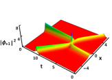
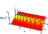
($a$)                                           ($b$)

Figure 13: ($a$) The elastic collision between two FS solitons with $\xi_{1}=0.2+\text{i}$, $\xi_{2}=-\text{i}$, $\Omega=-0.02$, $\theta_{01}=16$ and $\theta_{02}=0$. ($b$) The bound state of two nonautonomous FS solitons with $\xi_{1}=0.8\text{i}$, $\xi_{2}=0.4\text{i}$, $\Omega=-0.02$ and $\theta_{01}=\theta_{02}=0$.

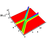
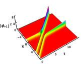
($a$) $A_{1}^{2}=50$                           ($b$) $A_{1}^{2}=500$

Figure 14: ($a$) The elastic collision between FS and PS solitons. ($b$) The inelastic collision between FS and PS solitons. The parameters are $\xi_{1}=0.2+\text{i}$, $\xi_{2}=\text{i}$, $\Omega=-0.02$, $\theta_{01}=16$, and $\theta_{02}=0$.

Next, we consider the interaction between FS and PS solitons with $\text{det}\Pi_{1}\neq 0$ and $\text{det}\Pi_{2}=0$, respectively, i.e., with different polarization matrices. For instance, with $A_{1}^{2}=4|\text{det}\Pi_{1}|^{2}=50$ the interaction is fully elastic, as seen in Fig. 14($a$). As it should be, under the action of the gain the amplitudes of the solitons grow exponentially. Interestingly, when the determinant of the polarization matrix $|\text{det}\Pi_{1}|$ decreases, that is, $A_{1}$ increases, inelastic interaction between the PS soliton and FS soliton occurs. For $A_{1}^{2}=500$, an example is shown in Fig. 14($b$). It is seen that the PS soliton changes into a single-hump soliton after the interaction with a FS soliton. In either case, the FS soliton remains unchanged after the collision.

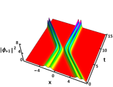
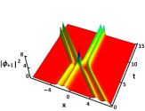
($a$) $A_{1}^{2}=50$                           ($b$) $A_{1}^{2}=500$

Figure 15: Shape-preserved interactions between two PS solitons with ($a$) $A_{2}^{2}=50$ ($b$) $A_{2}^{2}=500$. The parameters are chosen as $\xi_{1}=0.2+\text{i}$, $\xi_{2}=\text{i}$, $\Omega=-0.02$, $\theta_{01}=16$ and $\theta_{02}=0$.

Finally, we display the elastic collisions between two PS solitons in Fig. 15. It is seen that the two PS solitons keep their double-peak shapes intact after the interaction. Different from the interaction in Fig. 13($a$), no tall peak is observed in the interaction region in Fig. 15($a$). A general conclusion is that the polarization matrix $\Pi$ can control the strength of the inter-soliton interactions.

VI Conclusions

We have investigated the dynamics of nonautonomous matter-wave solitons in the spinor Bose-Einstein condensate subject to the spatiotemporal modulation. The model is based on the system of three nonlinearly coupled GP (Gross-Pitaevskii) equations with the time-dependent potential and gain-loss coefficient. We have derived the nonisospectral Lax pair with the time-dependent spectral parameter for this system, provided that the special integrability condition holds, given by Eq. (9). An infinite set of conservation laws is derived for the integrable system. Based on the Lax pair, the DT (Darboux transform) has been constructed and applied to generate one- and two-soliton solutions. By choosing several different external potentials and gain-loss coefficients, we have obtained various solutions for nonautonomous matter-wave solitons of both the ferromagnetic and polar types (with nonzero and zero total spin, respectively). These include the compressed, snakelike, and step-wise solitons, as well as breathers. We have utilized numerical simulation to analyze stability of the nonautonomous matter-wave solitons against random perturbations and found that both the ferromagnetic and polar solitons are stable. In particular, the evolution of the matter-wave solitons, resembling the creation of rogue waves, has been investigated under the action of the sign-reversible gain-loss distribution. We have also investigated elastic and inelastic collisions between nonautonomous matter-wave solitons, including ferromagnetic-ferromagnetic, ferromagnetic-polar, and polar-polar collisions. In particular, spin switching has been observed in the inelastic ferromagnetic-polar collisions. When the two solitons move at the same velocity, bound states of solitons have been obtained. The outcome of the interactions can be controlled by the solitons’ polarization matrices. Since the integrability condition of system (3) have been obtained, the dark non-autonomous solitons of system (3) with the repulsive interactions can also be derived via certain analytical method, and the results will be published elsewhere.

- [1] Anderson M. H., Ensher J. R., Matthews M. R., Wieman C. E., Cornell E. A., Observation of Bose-Einstein condensation in a dilute atomic vapor, Science 1995; 269:198.
- [2] Bradley C. C., Sackett C. A., Tollett J. J., Hulet R. G., Evidence of Bose-Einstein condensation in an atomic gas with attractive interactions, Phys. Rev. Lett. 1997;79:1170.
- [3] Mewes M. O., Andrews M. R., Druten N. J., Kurn D. M., Durfee D. S., Townsend C. G., Ketterle W., Collective Excitations of a Bose-Einstein Condensate in a Magnetic Trap, Phys. Rev. Lett. 1996;77:988.
- [4] Pitaevskii L., Stringari S., Bose-Einstein Condensation, Oxford University Press; 2016.
- [5] Malomed B. A., Multidimensional Solitons, AIP Publishing; 2022.
- [6] Kengne E., Liu W. M., Malomed B. A., Spatiotemporal engineering of matter-wave solitons in Bose–Einstein condensates, Phys. Rep. 2021;899:1.
- [7] Zhang Z., Chen L., Yao K. X., Chin C., Transition from an atomic to a molecular Bose–Einstein condensate, Nature 2021;592:708.
- [8] Musolino S., Kurkjian H., Van Regemortel M., Wouters M., Kokkelmans S., Colussi V. E., Bose-Einstein condensation of Efimovian triples in the unitary Bose gas, Phys. Rev. Lett. 2022;128:020401.
- [9] Henderson G. W., Robb G. R. M., Oppo G. L., Alison M. Yao, Control of light-atom solitons and atomic transport by optical vortex beams propagating through a Bose-Einstein Condensate, Phys. Rev. Lett. 2022;129:073902.
- [10] Pethick C. J., Smith H., Bose-Einstein Condensation in Dilute Gases, Cambridge University Press; 2008.
- [11] Kawaguchi Y., Ueda M., Spinor bose–einstein condensates, Phys. Rep. 2012;520:253.
- [12] Kartashov Y. V., Astrakharchik G. E., Malomed B. A., Torner L., Frontiers in multidimensional self-trapping of nonlinear fields and matter, Nat. Rev. Phys. 2019;1:185.
- [13] Malomed B. A., Mihalache D., Nonlinear waves in optical and matter-wave media: a topical survey of recent theoretical and experimental results, Rom. J. Phys. 2019;64:106.
- [14] Mihalache D., Localized structures in optical and matter-wave media: a selection of recent studies, Rom. Rep. Phys. 2021;73:403.
- [15] Li L., Li Z., Malomed B. A., Mihalache D., Liu W. M., Exact soliton solutions and nonlinear modulation instability in spinor Bose-Einstein condensates, Phys. Rev. A 2005;72:033611.
- [16] Li H., Zhu X., Malomed B. A., Mihalache D., He Y. J., Shi Z. W., Emulation of spin-orbit coupling for solitons in nonlinear optical media, Phys. Rev. A 2020;101:053816.
- [17] Stamper-Kurn D. M., Ueda M., Spinor Bose gases: Symmetries, magnetism, and quantum dynamics, Rev. Mod. Phys. 2013;85:1191.
- [18] Bersano T. M., Gokhroo V., Khamehchi M. A., D’Ambroise J., Frantzeskakis D. J., Engels P., and Kevrekidis P. G., Three-Component Soliton States in Spinor Bose-Einstein Condensates, Phys. Rev. Lett. 2018;120:063202.
- [19] Evrard B., Qu A., Dalibard J., Gerbier F., Observation of fragmentation of a spinor Bose-Einstein condensate, Science 2021;373:1340.
- [20] Kim K., Hur J., Huh S. J., Choi S., Choi J., Emission of spin-correlated matter-wave jets from spinor Bose-Einstein condensates, Phys. Rev. Lett. 2021;127:043401.
- [21] Vengalattore M., Leslie S. R., Guzman J., Stamper-Kurn D. M., Spontaneously modulated spin textures in a dipolar spinor Bose-Einstein condensate, Phys. Rev. Lett. 2008;100:170403.
- [22] Borgh M. O., Lovegrove J., Ruostekoski J., Internal structure and stability of vortices in a dipolar spinor Bose-Einstein condensate, Phys. Rev. A 2017;95:053601.
- [23] Ollikainen T., Masuda S., Mottonen M., Nakahara M., Counterdiabatic vortex pump in spinor Bose-Einstein condensates, Phys. Rev. A 2017;95:013615.
- [24] Meystre P., Atom Optics, Springer-Verlag; 2001.
- [25] Chen P. Y. P., Malomed B. A., Stable circulation modes in a dual-core matter-wave soliton laser, J. Phys. B: At. Mol. Opt. Phys. 2006;39:2803.
- [26] Sekh G. A., Pepe F. V., Facchi P., Pascazio S., Salerno M., Split and overlapped binary solitons in optical lattices, Phys. Rev. A 2015;92:013639.
- [27] Chai X., Lao D., Fujimoto K., Hamazaki R., Ueda M., Raman C., Magnetic solitons in a spin-1 Bose-Einstein condensate, Phys. Rev. Lett. 2020;125:030402.
- [28] Chai X., Lao D., Fujimoto K., Raman C., Magnetic soliton: From two to three components with SO(3) symmetry, Phys. Rev. Res. 2021;3:L012003.
- [29] Zhang X. F., Hu X. H., Liu X. X., Liu W. M., Vector solitons in two-component Bose-Einstein condensates with tunable interactions and harmonic potential, Phys. Rev, A 2009;79:033630.
- [30] Rajendran S., Muruganandam P., Lakshmanan M., Bright and dark solitons in a quasi-1D Bose–Einstein condensates modelled by 1D Gross–Pitaevskii equation with time-dependent parameters, Physica D 2010;239:366.
- [31] Yao Y. Q., Han W., Li J., Liu W. M., Localized nonlinear waves and dynamical stability in spinor Bose–Einstein condensates with time–space modulation, J. Phys. B 2018;51:105001.
- [32] Atre R., Panigrahi P. K., Agarwal G. S., Class of solitary wave solutions of the one-dimensional Gross-Pitaevskii equation, Phys. Rev. E 2006;73:056611.
- [33] Kevrekidis P. G., Theocharis G., Frantzeskakis D. J. Malomed B. A., Feshbach resonance management for Bose-Einstein condensates, Phys. Rev. Lett. 2003;90:230401.
- [34] Yan M., DeSalvo B. J., Ramachandhran B., Pu H., Killian T. C., Controlling condensate collapse and expansion with an optical Feshbach resonance, Phys. Rev. Lett. 2013;110:123201.
- [35] Enomoto K., Kasa K., Kitagawa M., Takahashi Y., Optical Feshbach resonance using the intercombination transition, Phys. Rev. Lett. 2008;101:203201.
- [36] Shen Y. J., Gao Y. T., Zuo D. W., Sun Y. H., Feng Y. J., Xue L., Nonautonomous matter waves in a spin-1 Bose-Einstein condensate, Phys. Rev. E 2014;89:062915.
- [37] Malomed B. A., Soliton Management in Periodic Systems, Springer; 2006.
- [38] Turitsyn S. K., Bale B. G., Fedoruk M. P., Dispersion-managed solitons in fibre systems and lasers, Phys. Rep. 2012;521:135.
- [39] Serkin V. N., Hasegawa A., Belyaeva T. L., Nonautonomous solitons in external potentials, Phys. Rev. Lett. 2007;98:074102.
- [40] Rajendran S., Lakshmanan M., Muruganandam P., Matter wave switching in Bose–Einstein condensates via intensity redistribution soliton interactions, J. Math. Phys. 2011;52:023515.
- [41] Yang Z. Y., Zhao L. C., Zhang T., Feng X. Q., Yue R. H., Dynamics of a nonautonomous soliton in a generalized nonlinear Schrödinger equation, Phys. Rev. E 2011;83:066602.
- [42] Wang D. S., Shi Y. R., Chow K. W., Yu Z. X., Li X. G., Matter-wave solitons in a spin-1 Bose-Einstein condensate with time-modulated external potential and scattering lengths, The Eur. Phys. J. D 2013;67:1.
- [43] Carr L. D., Brand J., Spontaneous soliton formation and modulational instability in Bose-Einstein condensates, Phys. Rev. Lett. 2004;92:040401.
- [44] Rowen E. E., Bar-Gill N., Pugatch R., Davidson N., Energy-dependent damping of excitations over an elongated Bose-Einstein condensate, Phys. Rev. A 2008;77:033602.
- [45] Ieda J., Miyakawa T. Wadati M., Exact analysis of soliton dynamics in spinor Bose-Einstein condensates, Phys. Rev. Lett. 2004;93:194102.
- [46] Serkin V. N., Hasegawa A., Belyaeva T. L., Nonautonomous matter-wave solitons near the Feshbach resonance, Phys. Rev. A 2010;81:023610.
- [47] Janis J., Banks M., Bigelow N. P., rf-induced Sisyphus cooling in a magnetic trap, Phys. Rev. A 2005;71:013422.
- [48] Gericke T., Würtz P., Reitz D., Langen T., Ott H., High-resolution scanning electron microscopy of an ultracold quantum gas, Nature Phys. 2008; 4(12): 949.
- [49] Würtz P., Langen T., Gericke T., Koglbauer A., Ott H., Experimental demonstration of single-site addressability in a two-dimensional optical lattice, Phys. Rev. Lett. 2009; 103(8): 080404.
- [50] Ablowitz M. J., Kaup D. J., Newell A. C., Segur H., Nonlinear-evolution equations of physical significance, Phys. Rev. Lett. 1973;31:125.
- [51] Rogers C. and Schief W. K.,Bäcklund and Darboux transformations, Cambridge University Press; 2002.
- [52] Chen Y. L., Representations and Cramer rules for the solution of a restricted matrix equation, Linear and Multilinear Algebra 1993;35:339.
- [53] Luo Z., Liu Y., Li Y., Batle J., Malomed B. A., Stability limits for modes held in alternating trapping-expulsive potentials, Phys. Rev. E 2022;106:014201.
- [54] El-Ganainy R., Makris K. G., Khajavikhan M., Musslimani Z. H., Rotter S., Christodoulides D. N., Non-Hermitian physics and PT symmetry, Nature Phys. 2018;14:11.
- [55] Dudley J. M., Genty G., Mussot A., Chabchoub A., Dias F., Rogue waves and analogies in optics and oceanography, Nature Rev. Phys. 2019;1:675.