EDEN Survey: Small Transiting Planet Detection Limits and Constraints on the Occurrence Rates for Late M Dwarfs within 15 pc

Abstract

Earth-sized exoplanets that transit nearby, late spectral type red dwarfs will be prime targets for atmospheric characterization in the coming decade. Such systems, however, are difficult to find via wide-field transit surveys like Kepler or TESS. Consequently, the presence of such transiting planets is unexplored and the occurrence rates of short-period Earth-sized planets around late M dwarfs remain poorly constrained. Here, we present the deepest photometric monitoring campaign of 22 nearby late M dwarf stars, using data from over 500 nights on seven 1-2 meter class telescopes. Our survey includes all known single quiescent northern late M dwarfs within 15 pc. We use transit-injection-and-recovery tests to quantify the completeness of our survey, successfully identify most ($>80\%$) transiting short-period (0.5-1 d) super-Earths (R $>1.9R_{\oplus}$), and are sensitive ($\sim$50%) to transiting Earth-sized planets (1.0–1.2 $R_{\oplus}$). Our high sensitivity to transits with a near-zero false positive rate demonstrates an efficient survey strategy. Our survey does not yield a transiting planet detection, yet it provides the most sensitive upper limits on transiting planets orbiting our target stars. Finally, we explore multiple hypotheses about the occurrence rates of short-period planets (from Earth-sized planets to giant planets) around late M dwarfs. We show, for example, that giant planets at short periods ($<$ 1 day) are uncommon around our target stars. Our dataset provides some insight into occurrence rates of short-period planets around TRAPPIST-1-like stars, and our results can help test planetary formation and system evolution models, as well as guide future observations of nearby late M dwarfs.

1 Introduction

Due to their intrinsic faintness, the in-depth characterization (beyond transit spectroscopy) of Earth-sized exoplanets will remain, for the foreseeable future, limited to the closest of planets – those that are within approximately 15 pc (e.g., Gaudi et al., 2020; The LUVOIR Team, 2019; Quanz, 2019; Apai et al., 2019). Although there are about 1000 stars in that volume (Gaia Collaboration et al., 2021) and likely at least 1 planet per star (e.g., Hardegree-Ullman et al., 2019), as of July 2022 only 175 planets have been confirmed, mostly via radial velocity (RV) measurements. Even in this small volume of the Milky Way surrounding us, a large fraction of planets remains undiscovered. Of the planets known, a rarely found type stands out: small planets ($R_{p}<1.8R_{\oplus}$) transiting small host stars ($R_{*}<0.4R_{\odot}$), which are ideal targets for transmission spectroscopic studies due to the deeper transits and generally higher signal-to-noise ratio (SNR) than planets around larger host stars.

Arguably, the best-suited terrestrial planets for in-depth spectroscopic studies, both due to their number and transit observability, are currently in the TRAPPIST-1 planetary system (Gillon et al., 2016, 2017). These seven approximately Earth-sized planets with similar or slightly lower densities than that of Earth (Agol et al., 2021) are orbiting a very late spectral type M dwarf (M8), near the stellar-substellar boundary. However, such low-mass stars are intrinsically very faint, limiting the feasibility of transit spectroscopy to systems that are very close to us (typically d $<15$ pc). Identifying a greater number of broadly TRAPPIST-1-like planetary systems would provide important opportunities for in-depth characterization of Earth-sized planets. Furthermore, a better understanding of the formation and evolution of these planets can provide context for the interpretation of incomplete data on their present-day atmospheres (e.g., Apai et al., 2018).

Yet, the occurrence rates and even the formation and evolution of these planetary systems remains poorly understood. Important population-level constraints emerged from the analysis of planetary systems around earlier spectral type stars that can be more readily studied via wide area transit surveys like Kepler (Borucki et al., 2010) and TESS (Ricker et al., 2015). With a small set of detected planets around mid-M dwarfs from Kepler data, Hardegree-Ullman et al. (2019) showed evidence for a higher occurrence rate of short-period (0.5–10 days) small planets (0.5–2.5 $R_{\oplus}$) for mid-M dwarfs ($1.19^{+0.70}_{-0.49}$ planets per star) than for early M dwarfs ($0.63^{+0.08}_{-0.06}$ planets per star), suggesting that the trend continues to the lowest mass stars, consistent with the lower limit on planet occurrence around late-M dwarfs implied by the detection of TRAPPIST-1 (Lienhard et al., 2020).

However, most current surveys studying planets around M dwarfs have some level of biases. Only 1% of the 186000 stars in the main Kepler sample, for example, are M dwarfs (Berger et al., 2020), so studies of transiting M dwarfs from Kepler (e.g., Dressing & Charbonneau, 2015; Mulders et al., 2015) are a biased sample, as these are likely only the brightest and earliest M dwarfs at a relatively far distance. The K2 stellar catalog had a larger sample of M dwarfs with $\sim 17\%$ of 220000 stars (Hardegree-Ullman et al., 2020), but this is still underrepresented as compared to the $\sim 70\%$ of stars in the galaxy that are M dwarfs (Henry et al., 2006) and again biased towards the larger, brighter M dwarfs. K2 studies of M dwarfs (e.g., Sagear et al., 2020; Sestovic & Demory, 2020) found no planets in a targeted sample list of $\sim 800-900$ stars, but this was not a blind volume-limited search, as it was guest-observer driven and therefore biased. RV surveys like CARMENES and HADES (Sabotta et al., 2021; Pinamonti et al., 2022, Ribas et al. (accepted)) are simply not sensitive to later M dwarfs with the current technological limits, as is also seen with the current TESS sample (see Figure 1).

Therefore, targeted surveys to detect exoplanets around mid-to-late-M dwarfs and early-L dwarfs like EDEN, MEarth (Irwin et al., 2009), SPECULOOS (Delrez et al., 2018; Sebastian et al., 2021) and PINES (Tamburo et al., 2022) are necessary to better understand planet occurrence near the substellar boundary. Even though their current detection numbers are low (less than 10 currently), these blind, volume-limited surveys still provide the least biased study of mid- to late-M dwarfs. Improved occurrence rate estimates are an important feedback for planet formation theories, which can be constrained by comparing synthesized planet populations to observed samples (e.g., Ida & Lin, 2004; Thommes et al., 2008; Mordasini et al., 2009; Ndugu et al., 2018; Izidoro et al., 2021; Schlecker et al., 2021a, b; Bitsch et al., 2021; Mulders et al., 2021; Kimura & Ikoma, 2022)

The Exoearths Discovery and Exploration Network (EDEN) is a global network of professional telescopes that works toward increasing our understanding of potentially habitable exoplanetary systems targeting the detection of, in particular, planetary systems within 15 pc. EDEN is led by four Co-PIs (D. Apai, P. Gabor, Th. Henning, W-P. Chen) on behalf of four institutions (Univ. Arizona, Vatican Observatory, Max Planck Institute for Astronomy in Heidelberg, and National Central University in Taiwan). A complementary, major survey component using research telescopes in Italy was led by L. Mancini (University of Rome “Tor Vergata”). EDEN began its full survey with seven research telescopes (diameters between 0.8–2.3 m) surveying nearby stars in 2018 for transiting planets. EDEN’s primary targets are late M dwarf stars beyond the reach of TESS (see Figure 1), and for these targets EDEN demonstrated sensitivity down to Earth-sized exoplanets (Gibbs et al., 2020). In this study, we observed over 500 nights on the northern late M dwarf population within 15 pc (with at least 25 hours per target) looking for transiting planets. In addition to its core transit search mission, EDEN also published studies of stellar flares and their impact on the habitability of the nearby star Wolf 359 (catalog ) (Lin et al., 2021), and contributed to many follow-up observations of TESS-identified planet candidates (Wells et al., 2021, Peterson et al., submitted; Pozuelos et al., submitted).

This paper is organized as follows. In Section 2 we describe the Project EDEN observing strategy, with the data reduction and detrending procedures shown in Section 3. We explain our analysis for the transit search and sensitivity in Section 4, and Section 5 contains the results of these analyses. Section 6 contains the implementation and results of our planet population hypothesis testing. Finally, in Section 7 we discuss our results from a population statistics perspective, as well as an unconfirmed signal, before summarizing our study in Section 8.

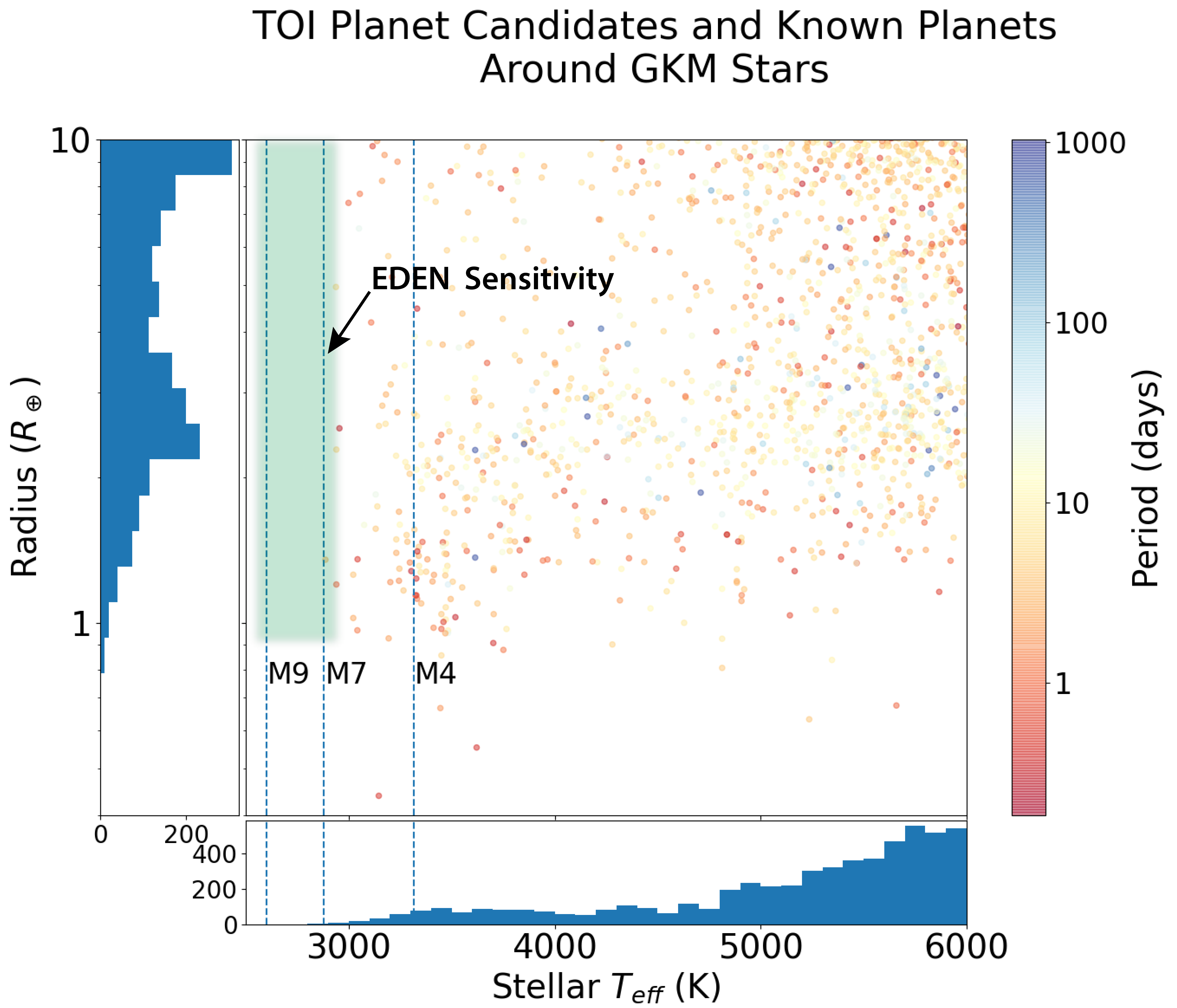
Figure 1: TESS objects of interest (TOIs) by stellar effective temperature and planet candidate radius. The temperature and planet radius distributions of the TOIs show a marked drop toward late spectral types ($>$M4–M6) and for small planets ($R_{p}<2$ $R_{\oplus}$). The green shaded region represents the sensitivity of our EDEN survey, which is complementary to that of TESS.

2 Observations

We continued EDEN observations as laid out in Gibbs et al. (2020). This section describes the key points of the observing strategy, including the procedure and the target stars for our survey.

2.1 Observing Process

We observed with seven telescopes across the northern hemisphere: four located in Arizona, two in Europe, and one in Taiwan (see Table 1 in Gibbs et al., 2020). Under ideal scheduling and weather conditions, this longitudinal coverage allows for continuous observations of target stars visible from all EDEN sites. The telescope apertures range in size from 0.8 m to 2.3 m. The Schulman 0.8 m telescope is robotically operated, while the CAHA 1.2 m is remotely operated. The rest require an on-site operator/observer each night. We took sky flat or dome flats, as well as bias frames, whenever possible. Dark frames are no longer acquired as we found no difference between data calibrated with or without darks, as the dark current is near zero at all telescopes and the targets have high SNR (Gibbs et al., 2020). We tried to observe a given target star for at least three hours per night, which is roughly three times the expected transit duration of a planet on a close-in orbit. This strategy allows us to observe multiple targets in one night if we cannot spend the entire night on one star (e.g., if the star is relatively southern and is only visible for half the night).

We used the GG495 filter from Schott, which is a long-pass filter that reaches 50% transparency at $\sim$500 nm and extends into the near-infrared, due to its greater transmission ($>90$%) than narrowband filters across visible and near-IR wavelengths. Some observations required a narrowband filter, usually due to moon brightness or for TESS transit follow-up. We usually used 60-s exposures unless the target was too bright/faint, or if higher time precision was required (e.g., transit timing variation (TTV) analysis of transit follow-up targets). In certain cases, we slightly defocused the star to both mitigate inter- and intra-pixel sensitivity differences and to avoid saturation for longer exposures on brighter targets (for further information see, e.g., Southworth et al., 2009; Gibbs et al., 2020).

Our detectors enter a non-linear regime of photon-electron counts at about 2/3 of the well limit; we thus aimed to stay below 60% of the full well level for bright targets. Our data reduction pipeline adjusts for saturation in the target and best reference stars, with brighter reference stars discarded if they are saturated. For most of our CCDs, the field-of-view is on the order of 10 arcmin, but the plate pixel scale differs, and in many cases the observations were binned in order to decrease readout time. We built our data reduction pipeline to be robust and agnostic to different plate scales, and only run photometry for one given night from one given telescope at a time.

2.2 Target Stars

The Project EDEN target list is comprised of all known single non-variable stars of spectral type M7–L0 within 15 pc and with declinations > -20^∘. At the beginning of our survey, we removed known binaries and active flare stars as indicated by SIMBAD from the 15 pc sample because they are likely to contaminate the light curve, making it more difficult to find a transiting planet. Once we removed the stars that do not fit the above criteria, we were left with 22 stars that became the focus of the survey.

It has been shown that the removal of binary stars from samples of demographic studies can introduce biases, mainly in the form of overestimating giant planet occurrence rates (Moe & Kratter, 2021). While close binaries may pose a threat to M dwarf planetary systems, they are relatively rare around low-mass stars (e.g., Shan et al., 2015; Susemiehl & Meyer, 2022). M dwarf binaries also tend to have 10$\times$ higher flare activity than single M dwarfs (Huang et al., 2020). The close binary fraction is also relatively constant across the M dwarf range, which suggests that there is no introduction of a systematic error with their removal (Offner et al., 2022). Additionally, M dwarf binary systems with planets or planet candidates tend to have wide separations between the stellar components (e.g., Clark et al., 2022a). To identify multiple stars in our sample, we searched the RECONS M dwarf binary catalogs (Winters et al., 2019; Vrijmoet et al., 2020), the Gaia EDR3 binary catalog (El-Badry et al., 2021), the recent results from Robo-AO (Salama et al., 2021, 2022), the M dwarf TESS objects of interest companion catalog (Clark et al., 2022a), and the POKEMON speckle catalog (Clark et al., 2022b). We found two binaries within our sample, EDEN Input Catalog (EIC) 10 and EIC 14.

Reiners & Basri (2009) identified EIC 10 (LP 775-031/Gaia DR3 3171631420210205056) as a double-lined spectroscopic binary (SB2) consisting of two nearly equal brightness components. Recent high-resolution imaging efforts have been unable to resolve the companion (Winters et al., 2019; Vrijmoet et al., 2020). Clark et al. (in prep) observed EIC 10 using speckle imaging, but were not able to resolve a companion. Speckle imaging is sensitive to separations $>0\farcs 1$, constraining the binary separation to $\lesssim 1$ au at a system distance of 10.6 pc. Indeed, Gaia DR3 revealed this target to have an orbital astrometric solution with a period of 105.56 days (Gaia Collaboration et al., 2022b). Assuming EIC 10 consists of two equal mass M7 stars ($0.09M_{\odot}$), Kepler’s third law places the component separation at 0.25 au, corresponding to $0\farcs 023$, below the sensitivity of speckle imaging.

Salama et al. (2022) identified EIC 14 (Gaia DR3 1097353325107339776) as a binary with an angular separation of $0\farcs 4$ and a $\Delta i^{\prime}$ magnitude of $2.28$, but the observation was conducted in 2012. Clark et al. (in prep) more recently resolved EIC 14 as a binary with an angular separation of $0\farcs 29$ and $\Delta 880$ nm magnitude of $1.62$. The angular separations at two different epochs place the binary companion between 3.5 and 5 au at a system distance of 12.3 pc. We kept this target in our sample due to the wide separation of the binary and implemented a flux correction factor (see 4.1).

Table 1: EDEN Observations of survey targets

EIC	Gaia DR3	RA (J2000)	Dec (J2000)	PM RA	PM Dec	Distance	Spectral	SpT	Hours
ID	ID	h:m:s	d:m:s	mas/yr	mas/yr	pc	Type	Ref.	Obs.
1	2091177593123254016	18:35:37.88	32:59:53.3	$-72.65\pm 0.05$	$-755.15\pm 0.05$	$5.689\pm 0.002$	M8.5V	[1]	204.0
2	56252256123908096	3:20:59.71	18:54:22.8	$352.29\pm 0.09$	$-257.07\pm 0.08$	$14.648\pm 0.017$	M8V	[2]	324.8
4	2531195858721613056	1:09:51.20	-3:43:26.4	$372.17\pm 0.27$	$8.65\pm 0.16$	$10.568\pm 0.023$	M9Ve	[3]	176.2
5	31235033696866688	3:14:03.44	16:03:05.5	$-242.96\pm 0.19$	$-54.85\pm 0.16$	$13.768\pm 0.036$	L0	[4]	100.0
6	445100418805396608	3:30:48.89	54:13:55.2	$-151.99\pm 0.04$	$3.42\pm 0.04$	$10.502\pm 0.004$	M7V	[5]	47.9
7	3257243312560240000	3:51:00.03	-0:52:44.9	$10.99\pm 0.06$	$-469.97\pm 0.05$	$14.678\pm 0.015$	M8.0V	[6]	47.5
8	230171768457140736	3:57:19.98	41:07:42.6	$-204.37\pm 0.06$	$-24.74\pm 0.05$	$14.183\pm 0.012$	M7V	[5]	106.4
9	229155579195699456	4:19:52.13	42:33:30.4	$528.67\pm 0.08$	$-1441.61\pm 0.06$	$10.262\pm 0.010$	M8.5V	[1]	411.3
11	3200303384927512960	4:40:23.27	-5:30:08.1	$334.53\pm 0.06$	$127.91\pm 0.06$	$9.747\pm 0.006$	M7	[8]	49.1
12	3421840993510952192	5:10:20.09	27:14:01.9	$-213.27\pm 0.08$	$-630.81\pm 0.06$	$10.276\pm 0.007$	M7V	[5]	213.0
13	191109281417914880	5:39:24.80	40:38:42.8	$646.15\pm 0.09$	$-834.49\pm 0.05$	$11.367\pm 0.010$	M8.0	[1]	49.4
14	1097353325107339776	8:25:52.82	69:02:01.1	$-691.17\pm 0.29$	$-1276.32\pm 0.39$	$12.289\pm 0.059$	M7V	[5]	57.0
15	5761985432616501376	8:53:36.16	-3:29:32.2	$-516.61\pm 0.08$	$-199.65\pm 0.05$	$8.659\pm 0.005$	M9.0	[1]	65.1
16	1227705135863076864	14:28:04.16	13:56:13.3	$-365.42\pm 0.06$	$-495.51\pm 0.06$	$13.230\pm 0.010$	M7V	[5]	57.3
17	1287312100751643776	14:28:43.23	33:10:39.3	$-346.96\pm 0.04$	$-710.99\pm 0.09$	$10.969\pm 0.012$	L0	[9]	219.8
18	1282632682337912832	14:44:17.18	30:02:14.2	$-94.39\pm 0.07$	$-340.33\pm 0.07$	$14.781\pm 0.015$	M8e	[10]	80.2
19	1262763648230973440	15:01:08.19	22:50:02.1	$-43.12\pm 0.11$	$-65.14\pm 0.14$	$10.734\pm 0.016$	L0	[9]	64.5
20	1272178319624018816	15:24:24.76	29:25:31.5	$-56.77\pm 0.03$	$-629.24\pm 0.04$	$13.078\pm 0.008$	M7.5V	[2]	95.7
21	6265453524968112640	15:34:56.93	-14:18:49.3	$-918.81\pm 0.14$	$-330.23\pm 0.10$	$10.938\pm 0.013$	M8.6V	[7]	45.4
22	4588438567346043776	18:26:11.00	30:14:18.9	$-2290.75\pm 0.09$	$-683.27\pm 0.09$	$11.101\pm 0.010$	M8.5V	[11]	80.2
23	1762523981210977664	20:44:37.48	15:17:34.8	$303.68\pm 0.06$	$-155.49\pm 0.05$	$10.395\pm 0.006$	M8	[12]	27.4

Notes: TRAPPIST-1 observed in follow-up program. Distance and proper motion values from Gaia DR3 (Gaia Collaboration et al., 2022a). Spectral type references are [1]: Reiners et al. (2018), [2]: Kirkpatrick et al. (2011), [3]: Henry et al. (2018), [4]: Smart et al. (2017), [5]: Newton et al. (2014), [6]: Deshpande et al. (2012), [7]: Bardalez Gagliuffi et al. (2014), [8]: Faherty et al. (2009), [9]: Kiman et al. (2019), [10]: Gizis et al. (2000), [11]: Lépine et al. (2002), [12] Photometric type from Reylé (2018).

Table 2: Apparent magnitudes of the EDEN targets presented in this study.

EIC	G	eG	J	eJ	H	eH	K	eK
ID	$\mathrm{mag}$	$\mathrm{mag}$	$\mathrm{mag}$	$\mathrm{mag}$	$\mathrm{mag}$	$\mathrm{mag}$	$\mathrm{mag}$	$\mathrm{mag}$
1	14.8510	0.0029	10.270	0.022	9.617	0.021	9.171	0.018
2	16.1048	0.0032	11.759	0.021	11.066	0.022	10.639	0.018
4	16.3750	0.0031	11.694	0.021	10.931	0.026	10.428	0.025
5	17.2427	0.0035	12.526	0.024	11.823	0.036	11.238	0.021
6	13.7143	0.0028	10.173	0.021	9.595	0.016	9.284	0.018
7	15.3131	0.0028	11.302	0.024	10.609	0.022	10.232	0.024
8	14.6381	0.0029	10.903	0.023	10.299	0.020	9.949	0.019
9	15.5551	0.0028	11.094	0.022	10.383	0.028	9.900	0.022
11	14.9043	0.0029	10.658	0.024	9.986	0.022	9.545	0.019
12	14.9257	0.0030	10.698	0.020	9.965	0.022	9.560	0.018
13	15.2733	0.0029	11.109	0.021	10.446	0.021	10.044	0.018
14	13.7621	0.0038	10.078	0.021	9.496	0.019	9.161	0.014
15	15.8889	0.0030	11.212	0.026	10.469	0.026	9.942	0.024
16	14.8963	0.0029	11.014	0.021	10.390	0.015	10.026	0.020
17	16.6346	0.0028	11.990	0.021	11.225	0.029	10.744	0.024
18	15.9061	0.0029	11.671	0.020	11.017	0.021	10.616	0.018
19	16.5353	0.0030	11.866	0.022	11.181	0.030	10.706	0.024
20	15.2801	0.0028	11.206	0.022	10.535	0.021	10.155	0.015
21	15.7637	0.0029	11.380	0.023	10.732	0.022	10.305	0.023
22	15.9470	0.0030	11.659	0.020	11.175	0.016	10.811	0.019
23	15.2678	0.0028	11.025	0.022	10.490	0.016	10.061	0.018

Notes: Gaia magnitudes from DR3 (Gaia Collaboration et al., 2022a), JHK magnitudes from 2MASS (Skrutskie et al., 2006)

The sample of stars matching our criteria (including the wide-separation binary) is shown in Tables 1 and 2. As the completeness of our targets within 15 pc neared 100% during the survey, we extended our observations to stars in the 15–21 pc range, as well as many targets outside the criteria (either in distance or in spectral type) as interesting candidates during the time when no $<$15 pc target was seasonally observable, as well as interesting candidates for other scientific purposes (e.g., the high-frequency flare star Wolf 359; Lin et al., 2021). These targets are shown in Table 3. In addition, we performed targeted follow-up observations of exoplanet candidate stars found by TESS (see Table 4).

3 Data Reduction

Here we provide a summary of our photometric pipeline edenAP and additional post-processing steps we took to prepare the data for our transit search.

3.1 Photometric Pipeline

We began our photometric process by calibrating the target frames using combined flats and biases. This step is coded to be optional in case of bad or unavailable calibration files, which only rarely occurs ($<5\%$ of nights) and does not significantly reduce the quality of our light curves. We then performed aperture photometry using photutils (Bradley et al., 2019), including calculating an astrometric solution using astrometry.net (Lang et al., 2010). We selected the aperture size between 5-50 pixels in steps of 1 pixel that minimizes the RMS scatter in the light curve of the target and a sky background median value of a 60x60 pixel box around the target after other sources are removed. Finally, we ran a simple comparison detrending of the light curve. The six reference stars in the field (or as many as possible in the rare cases where there are few reference stars) with the lowest average deviation within bins of 20 exposures across the light curve were median-combined into a single unbinned light curve, which was then divided out from the target light curve (see e.g., Gibbs et al., 2020, Section 3.4). Further detrending was performed as part of the transit search, as described in the following section.

3.2 Light Curve Detrending

As is usual for ground-based, high-precision photometry, our data are impacted by relatively slowly changing systematics, usually arising from airmass changes, telescope positional drift, and seeing variations. In order to correct for these systematics, we performed detailed detrending analysis similar to that laid out in Section 4.2 of Gibbs et al. (2020). Specifically, we followed these steps:

• We divided the normalized light curve by a 2nd-order polynomial that we fit to the original data.

• We performed a median filter over a 2 hour window.

• We removed any data points 2$\sigma$ above the median but not below to avoid removing transits much shorter (1-2 hours) than the length of the overall light curve ($>$3 hours).

• We fit a 2nd-order multivariate polynomial, based on the airmass, background level, and pixel x-y positions and divided it out.

Although we adopted steps from Gibbs et al. (2020), we also explored whether alternative detrending approaches may yield better results. Specifically, we tested multiple detrending procedures from the Wōtan package (Hippke et al., 2019), including combinations of biweight filtering, median filtering, spline fitting, and Savitsky-Golay polynomial fitting. For injected planet transit tests, none of the above versions of detrending procedures provided a lower scatter in the out-of-injected-transit baselines without also overfitting and at least partially removing the injected transit from the dataset. Specifically, the biweight filtering is best at removing signals from the raw dataset that have much longer timescales than the transit signal. For short-timescale signals across the duration of one observing night, biweight filtering did not improve the results. Therefore, our tests did not demonstrate that alternative approaches result in significant improvement, and we thus decided to continue using our original detrending procedure.

3.3 Variable Precipitable Water Vapor

A potential source for false positive detections are variations of precipitable water vapor (PWV) in Earth’s atmosphere, in particular for red target stars such as the ones in our survey (e.g., Bailer-Jones & Lamm, 2003; Blake et al., 2008). These variations may affect the accuracy of photometric time series in magnitudes and time scales that could be comparable to transit signals (Berta et al., 2012).

The filter bands in which EDEN observations are done are sometimes affected by PWV, as they overlap with several water vapor bands. The magnitude of the light curve impairment due to PWV depends on the spectral energy distributions of the target and comparison stars, the amount of water vapor in the atmospheric column along the line of sight of the telescope and its variation in time, and the bandwidth and wavelength of the used filters. Mitigation strategies have been put forward, such as evaluating the contribution of PWV across global, all-sky light curves and/or monitoring using local environmental sensors (Pedersen et al., 2023), as well as concurrent satellite remote sensing observations to drive a correction (Meier Valdés et al., 2021).

Given the above, PWV — if it affects LCs significantly – is expected to introduce false positives. However, there is no evidence for such effect in our dataset: the fact that we only detected one transit candidate (see Sect. 7.2) in $>2450$ hours of photometry shows that PWV is not a major source of false positives for the combination of filter choice and telescope locations of the EDEN survey. However, in the case of a signal that survives initial validation steps, we will need to evaluate the possibility of a false positive scenario caused by PWV.

4 Analysis

4.1 Transit search

We first analyzed all the data we had on each target by eye via the EDEN Interactive Viewer, which shows the light curve for the night along with airmass, moon altitude, sky background, reference and target star flux, and x-y pixel positions. Transit-like features were manually flagged for potential follow-up, but most variations in the data can be attributed to observing conditions or stellar activity. We account for the dilution of potential transit depths from the binary star EIC 14 by implementing a correction factor following Equation 4 from Furlan et al. (2017), with $\Delta m=1.62$). We note that our GG495 long-pass filter is not the same as the narrow-band 880 nm of the speckle observations, making this $\Delta m$ value an approximation. Assuming a planet orbits the primary, brighter star in the system, the correction factor is $\sim$1.1.

To more thoroughly search for signatures of planetary transits in EDEN photometry, we used the Transit Least Squares (TLS; Hippke & Heller, 2019) search algorithm, which is based on a template signal shape informed by small-planet detections of the Kepler mission. We applied the algorithm on all stars in our sample with data cuts at 0.3%, 0.6%, 0.9%, and 10% precision levels. Each of these runs returns a periodogram, model light curve (including phase folding), and best-fit parameters (period, duration, depth/radius ratio, mid-transit time for first transit in our data, and false alarm probability) for the expected transits. We note that TLS always attempts to fit a transit model, and that many of the output parameters are likely not actual transits but instead false positives that are the result of attempting to fit a transit to short-period and short-duration noise residuals in the light curves. We vetted all the signals and discarded any transit models with high false alarm probability ($>0.01$) as well as those signals with low false alarm probabilities but with parameters for planets that are unlikely to exist and be detected with our observations: transit durations $\lesssim$15 minutes, orbital periods $<0.25$ days, transit depths corresponding to planets $<0.1R_{\oplus}$.

4.2 Detection sensitivity

In order to probe the underlying planet population through our detection statistics, a thorough understanding of our survey completeness is necessary. Besides the geometric probability of a planet to transit given our line of sight to its host star, the completeness of our survey is limited by our ability to detect transit signatures. Our sensitivity is mostly limited by the photometric precision of our light curves and by the performance of our detection pipeline.

For close-to-ideal surveys not suffering from non-uniform sampling and significant data gaps, analytic expressions exist to estimate the sensitivity for transit signals (e.g., Pepper et al., 2003). In the case of our ground-based survey with its inevitable irregularities, we instead employed injection-and-retrieval simulations. Our approach was to inject planet signatures on a grid in the orbital period and planet radius and recover them. We used a log-spaced grid of 20 orbital period bins from 0.5-10 days, but if we had less than 10 nights of data on a target we truncated the grid to the number of nights we had. We also used a log-spaced grid of 12 planet radius bins from $0.6-3.5\,R_{\oplus}$. For the targets with data covering less than 10 nights, we artificially cut off the injections to periods where we would see at least two transits of the injected planet.

We created 250 planets with a random orbital period, orbital phase, and planet radius within each of the given grid bins, where the random values were drawn from a uniform distribution within each bin. This differs from the process in Gibbs et al. 2020, where they injected enough planets to retrieve 10 observable transiting planets per bin. This is due to increased noise levels generated by the previous method (see Figure 5 in Gibbs et al. 2020). In addition, we assumed the orbits to be circular, we randomly drew the impact parameter from a uniform distribution between 0 and 0.7 to avoid grazing transits, and we used the Claret (1998) limb-darkening law with coefficients $u_{1}=0.84$ and $u_{2}=0.125$. We injected the transit signals of each artificial planet into our observed photometric time series, detrended the resulting light curve, and ran the TLS algorithm to attempt to recover the injected planets. An example detrended light curve with an injected transit is shown in Figure 2. The results of our transit search are described in Section 5.2.

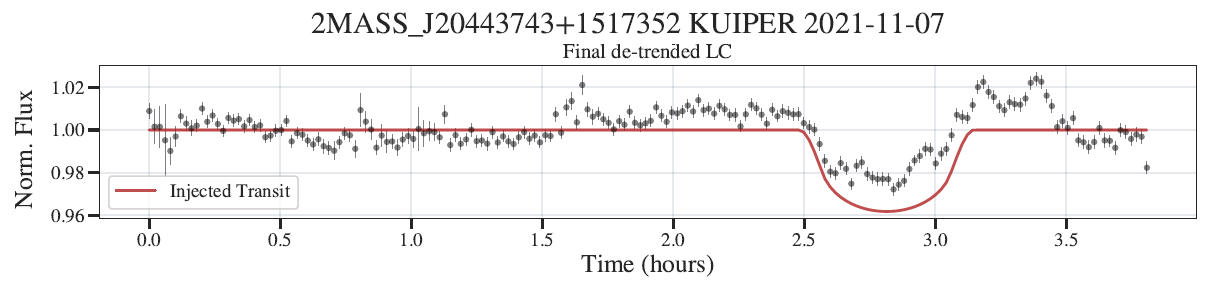
Figure 2: A detrended light curve with an injected transit from the Kuiper 61” telescope on 07 Nov 2021 UT. The transit is deep enough that the detrending raises the baseline pre- and post-transit slightly compared to the rest of the light curve, but this does not affect our ability to recover the injected planet because it is such a strong signal (SNR $\sim$ 6).

We considered our injected planets to be detected and positively recovered if the period was within 0.02 days (or 24 minutes) of the injected period, which corresponds to a fractional difference $\leq 4\%$ based on the actual given period. We also accounted for undersampled periods due to the scarcity of our data by looking at light curves with at least 2 transits found and checking to see if the given period for the injected planet still matched the injected transits recovered. We created a separate detection filter for single transits found and discarded those, as we cannot place our desired constraint on the orbital period of a planet with only one transit recovered.

5 Results

5.1 High-precision light curves for the EDEN Targets

Our survey yielded a rich dataset of detrended light curves with $\sim 1-10\,\mathrm{mmag}$ scatter for 22 EDEN target stars ranging in spectral types from M7V to L0, and in distance from 5.7 pc to 14.8 pc. For most target stars, our dataset provides the highest quality photometric monitoring to date, often with a unique combination of relatively high cadence ($\sim$60 seconds), sensitivity, and monitoring baseline. The light curves were used in this study to search for transiting exoplanets and place upper limits on their occurrence rates, but they can also be exploited for studies of stellar activity and stellar rotation, among other uses (see e.g., Lin et al., 2021; Murray et al., 2022). Although not included here, our dataset also provides similar photometric monitoring information for typically a dozen other stars in the same field of view of our target stars.

5.2 Transit Search

Our careful manual and algorithmic analyses of the light curves resulted in no convincing transit detections. Roughly 20 potential transit signals were flagged in all of our data, and there was one repeating, transit-like signal, which we followed up with additional observations and found no further evidence of a transit (see Section 7.2). Many TLS results were discarded as being unphysical false positives via the vetting procedure mentioned in Section 4.1. Therefore, we conclude that TLS found no real transit signals in the data from any of our targets. The fact that our light curves did not show many false positives — yet remained very sensitive to exoplanets down to Earth-radii — demonstrates the efficiency of our data reduction and analysis approach.

5.3 Detection sensitivity

We report the percentage of planets recovered with properties similar to the injected ones and created a map of the recovery probability in our sensitivity maps (see Figure 3 for the average map and full detection probability from the EDEN survey and Appendix A for the full set of 22 sensitivity maps).

Our average sensitivity to approximately Neptune-sized planets ($R\sim 3.5R_{\oplus}$) on very short ($P\sim 0.5$ days) orbits for most of our target stars is $\sim 85-90\%$ (see the top left corner of the top panel of Figure 3), which can be extended as a conservative estimate to larger planets as well. Due to the nightly cadence of observations, we tend to see a higher sensitivity for our targets at periods that are integer multiples of one day. Overall, our light curves are very sensitive to short-period ($P<1.5$ days) super-Earths and larger ($R>1.5R_{\oplus}$) exoplanets and, for most of our targets, we can exclude that such transiting planets orbit our targets.

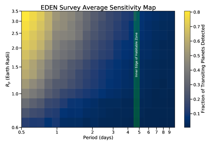
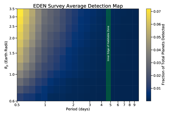
Figure 3: The average sensitivity (top) and full detection probability including geometric transit likelihood (bottom) of the EDEN survey for planets with periods between 0.5 and 10 days and sizes between 0.6 and 3.5 Earth radii. For ultra-short-period planets ($<$ 1 day), we reach 50% sensitivity for planets with radius $1.5R_{\oplus}$ or larger. Due to the low geometric transit probability, the overall completeness is much lower and drops sharply with the orbital period. The inner edge of the habitable zone is defined using the Kopparapu et al. (2013) model based on the temperature and insolation (assuming a stellar effective temperature of 2600 K and a planetary albedo of 0.3).

We note that EIC 7 (2MASS J05310004-0052452) and EIC 21 (2MASS J15345704-1418486) have significantly lower sensitivity than the other targets, which occurs due to a combination of low overall time observed (<50 hours), a southern declination, and relatively high light curve scatter for more observations than other targets. However, these two targets do not significantly affect the overall average sensitvity map, and we include them here for completeness.

6 Population-Level Insights

Our well-characterized sensitivity and relatively large sample size allow us not only to provide robust upper limits in a previously poorly explored region of the parameter space, but also to contrast the outcome of our survey (no planet detection) to different hypothetical planet populations. In the following analysis, we explored two demographic features: First, we analyzed the occurrence rate of TRAPPIST-1 b analogs and TRAPPIST-1-like planetary systems. Second, we analyzed the occurrence rate of close-in ($P\lesssim 1$ day) giant planets.

In both cases, we used the survey completeness described in Section 4.2 to compare our results to a hypothetical planet population. This approach follows the Monte Carlo assessment method introduced in Kasper et al. (2007) to contrast non-detections from a direct imaging survey with possible extrapolations of the exoplanet population detected by radial velocity surveys to larger separations. Since then, this method has been used for a variety of similar applications (e.g., Mulders et al., 2018).

This approach – forward-modeling and quantitative comparison to the predictions – is generally preferable to the inversion of sensitivity maps to occurrence rates for two reasons: (1) it allows for a more accurate consideration of sensitivity differences between individual targets and for a better handling of the subtleties of the observational biases; and (2) it provides more robust results for parameter ranges with only a few detections. For a detailed discussion of the advantages of this approach, see Mulders et al. (2018).

In this implementation of the Monte Carlo assessment, we simulated observations of synthetic planets in the measured EDEN light curves, with the planet parameters drawn from model distributions corresponding to the specific hypothesis tested - for example, a TRAPPIST-1 b-like planet would be a 1.1 $R_{\oplus}$ planet orbiting at P = 1.5 days with a random inclination. We then determined in what fraction of the simulated surveys the number of detections would be consistent (at $2\sigma$) with the outcome of the EDEN survey. For example, if our survey resulted in zero planet detections, but our hypothesis would lead to planet detections in 95% of the simulated surveys, we would be able to exclude that hypothesis at a 95% confidence level.

We also performed an upper-limit analysis for the occurrence rates following the procedure by Sagear et al. (2020). We set the probability of detecting zero planets to a given value (here 0.05) and then calculated the occurrence rate necessary to reach that null detection probability, given our detection sensitivities for each target star (see Equation 3 in Sagear et al., 2020). The results from our analysis are shown in Figure 4. We find that we have similar results to the upper limits from Sagear et al. (2020) when adjusting for their different bin sizes and types (log-linear vs log-log in orbital period and planet radius) for, e.g., mini-Neptune planets with orbital periods just greater than 1 day. We also provide detailed upper limits for short-period ($<1$ day) planets down to 0.6 $R_{\oplus}$. These values are also similar to the occurrence rates from Sestovic & Demory (2020). While the K2 occurrence rates were indeed slightly more limiting, they came from a biased sample of M dwarfs chosen by users instead of a volume-complete sample, so our work complements and extends that of previous studies to this nearby sample.

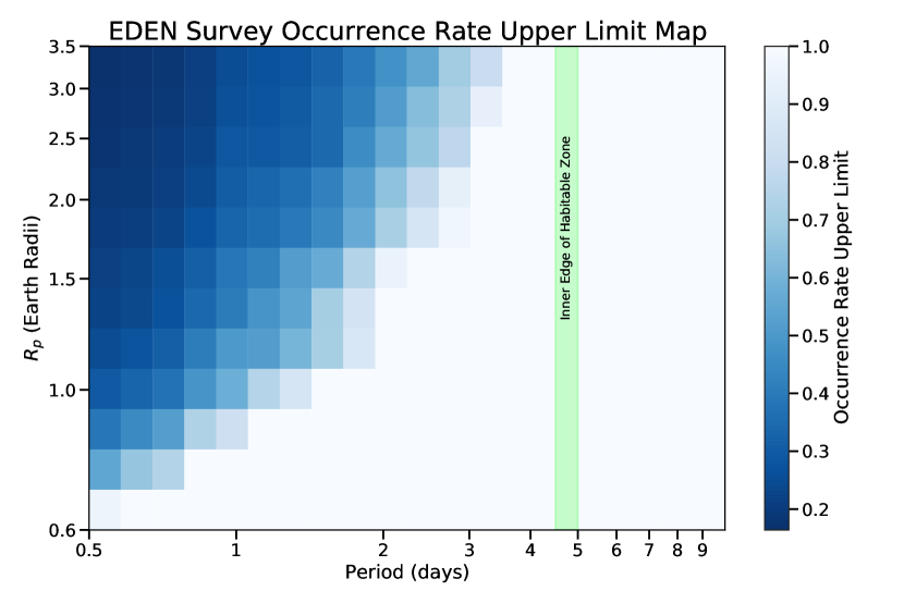
Figure 4: The upper limit on the occurrence rate from our analysis that follows the procedure from Sagear et al. (2020), assuming $P_{null}=0.05$. We find similar occurrence rates when adjusting for bin size and type (log-linear vs log-log in orbital period and planet radius) for, e.g., mini-Neptune planets with orbital periods just greater than 1 day.

6.1 The Occurrence Rate of TRAPPIST-1 b Analogs and TRAPPIST-1-like Planetary Systems

Using the above-described Monte Carlo method to statistically compare the results of simulated surveys of hypothetical exoplanet populations to the actual results of our survey, we first tested the hypothesis that “TRAPPIST-1 b analogs orbit every late M dwarf star”, or $f_{\mathrm{Trb}}=100\%$. Although simplistic, this hypothesis is a sensible starting point for the exploration of the exoplanet population around late M dwarfs, since short-period planets like TRAPPIST-1 b are among the easiest to detect in the known late M dwarf population.

In order to do so, we simulated our EDEN transit survey 10,000 times to determine in what fraction of these surveys would the predicted results be consistent with our actual survey. Assuming isotropic orbit orientations, we injected a planet with a probability $P_{\mathrm{geom}}=(R_{\star}+R_{p})/a$, which approximates the geometric transit probability for a planet with radius $R_{p}$ on a circular orbit with semi-major axis $a$ around a star with radius $R_{\star}$. In the case of a transit occurring, we injected the photometric signature of a planet with random orbital phase and TRAPPIST-1 b’s orbital period and planet radius (P=1.511 days, R=1.116 $R_{\oplus}$; Agol et al., 2021) and tested its detection by our pipeline. In 15% of our simulated surveys, we would have seen at least one planet out of our sample of 22 stars. Our sensitivity (probability to detect a transiting TRAPPIST-1 b) is $\sim 18\%$, whereas the completeness (probability of detecting a planet, so the sensitivity multiplied by the geometric transit probability) is $\sim 0.8\%$.

We also tested the hypothesis that “TRAPPIST-1-like planetary systems orbit every late M dwarf star” ($f_{\mathrm{Tr}}<100\%$) as an extension to the TRAPPIST-1 b hypothesis. The additional planets in the full TRAPPIST-1 system make the system as a whole more likely to be discovered, even with individual planets decreasing in detection likelihood going outwards in the system. We took all of the planet period and radius values from Agol et al. (2021), and set a random system inclination and a Rayleigh distribution for mutual inclinations around $2^{\circ}$ (e.g., Fabrycky et al., 2014, although Luger et al. 2017 measured the TRAPPIST-1 mutual orbital inclinations to be around 0.3^∘). Planets g and h were included, but with the survey sensitivity as if they were at an orbital period of 10 days because their orbital periods are beyond 10 days. Again the EDEN transit survey was simulated 10,000 times, and in 21% of the surveys we would have detected at least one planet.

6.2 Giant Planet Occurrence Rates

In the following, we provide an estimate of the occurrence rate of close-in giant planets around late M dwarfs based on our survey’s completeness in this parameter domain. Our constraint is based on the same numerical Monte Carlo experiment as above for TRAPPIST-1 b analogs. As a conservative approximation, we assumed for these planets the sensitivity we found for the largest artificial planets that we injected in our sensitivity analysis ($3.5\text{\,}\mathrm{R}_{\oplus}$, see Section 4.2). For a host star radius representative of an M8V dwarf ($R_{\star}=0.114\,R_{\odot}$; Pecaut & Mamajek, 2013), the geometric transit probability $P_{geom}\approx$11\text{\,}\mathrm{\char 37\relax}$$ for a planet on a $1.05\text{\,}\mathrm{d}$ orbit. Even assuming such close orbits, $98\text{\,}\mathrm{\char 37\relax}$ of our mock surveys yield zero detections if giant planets occur around $2\text{\,}\mathrm{\char 37\relax}$ of late M dwarfs (Ghezzi et al., 2018). If instead every such star hosts a giant planet, we would expect to detect at least one giant planet in our survey in $73\text{\,}\mathrm{\char 37\relax}$ of the cases. If we decrease the orbital period down to $0.5\text{\,}\mathrm{d}$ orbital periods, the average sensitivity to a transiting planet increases by a factor of $\sim 1.6$, and we can constrain the giant planet occurrence rate down to $75\text{\,}\mathrm{\char 37\relax}$ with 95% confidence.

7 Discussion

7.1 Light curves

Our EDEN observations provide the most extensive set of light curves for the majority of our 22 target stars. Table 1 summarizes our targets and the total length of observations for each. Even though our targets are close to the Solar System ($d<$15 pc), the majority of the target stars are too faint for wide-array or all-sky surveys – such as HAT (Bakos et al., 2002), MEarth (Irwin et al., 2009), or TESS (Ricker et al., 2015) – to search for planets. For example, a comparison of our targets (with typical spectral types of M7–M9) to the stellar effective temperature and planet radius distribution of TESS Objects of Interest (TOI) as of April 2022 (see Figure. 1) illustrates how well our observations complement the TESS survey: there are currently no TOIs with spectral types beyond M7. This paucity of TOIs for late spectral types is primarily due to the fact that TESS’s sensitivity – in spite of extreme photometric stability – is limited to brighter stars by its small collecting area. The MEarth project, which utilized arrays of small robotic telescopes to search for transiting planets around bright mid-to-late M dwarfs (Nutzman & Charbonneau, 2008), reports photometric precisions of $0.2\text{\,}\mathrm{\char 37\relax}1.0\text{\,}\mathrm{\char 37\relax}$ at a typical cadence of $\sim$25\text{\,}\mathrm{min}$$ (Berta et al., 2013).

In comparison to these other current M dwarf surveys, the EDEN survey, due to the large apertures and uniform observing and data reduction strategy, accomplishes both uniquely long monitoring with high cadence and high sensitivity. Specifically, our targets are observed for at least 25 hours (the equivalent of about four typical, clear nights) and 1/3 of our targets were observed for over 100 hours (the equivalent of about 15 typical, clear nights) with $\sim$60 second cadence. As the light curves collected in our EDEN survey will likely be of use for a variety of future studies (e.g., stellar activity and rotation measurements), we make the reduced and calibrated light curves available to the community as an online data set accompanying this paper. The non-EDEN targets observed in our survey (Tables 3 and 4) represent a less homogeneous dataset. Those light curves and the ensemble of images obtained are available on a collaborative basis and will be made fully available in the near future.

7.2 A possible signal on EIC 9 (2MASS J04195212+4233304)

During observation runs in fall-winter 2020, we identified transit-like features in light curves of EIC 9 (2MASS J04195212+4233304), a 0.5-1% dip with a duration of $\sim$45 minutes. Similar features occurred twice on the same day of 18 Nov 2020 (UT), once observed by the Lulin One-meter Telescope (LOT) in Taiwan and again about 14 hours later by the Kuiper 61" Telescope in Arizona. The Vatican Advanced Technology Telescope (VATT) in Arizona observed another feature on 22 Dec 2020 (UT). The VATT and Kuiper features were both 1% depths, whereas the LOT feature was 0.5%, and the LOT and Kuiper features were both $\sim 40-45$ minutes in duration, whereas the VATT feature was $~{}\sim 60$ minutes (see Figures 5 and  6). The weather at the site for all three events was nominal - no clouds during the LOT and VATT events, and light cirrus at the Kuiper in the east as the target was setting. Our observations are done with intra-exposure guiding every few seconds on a bright star near the target, and there were no guiding errors during the observations so the target and reference star centroids remained consistent.

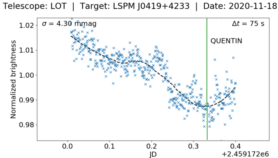
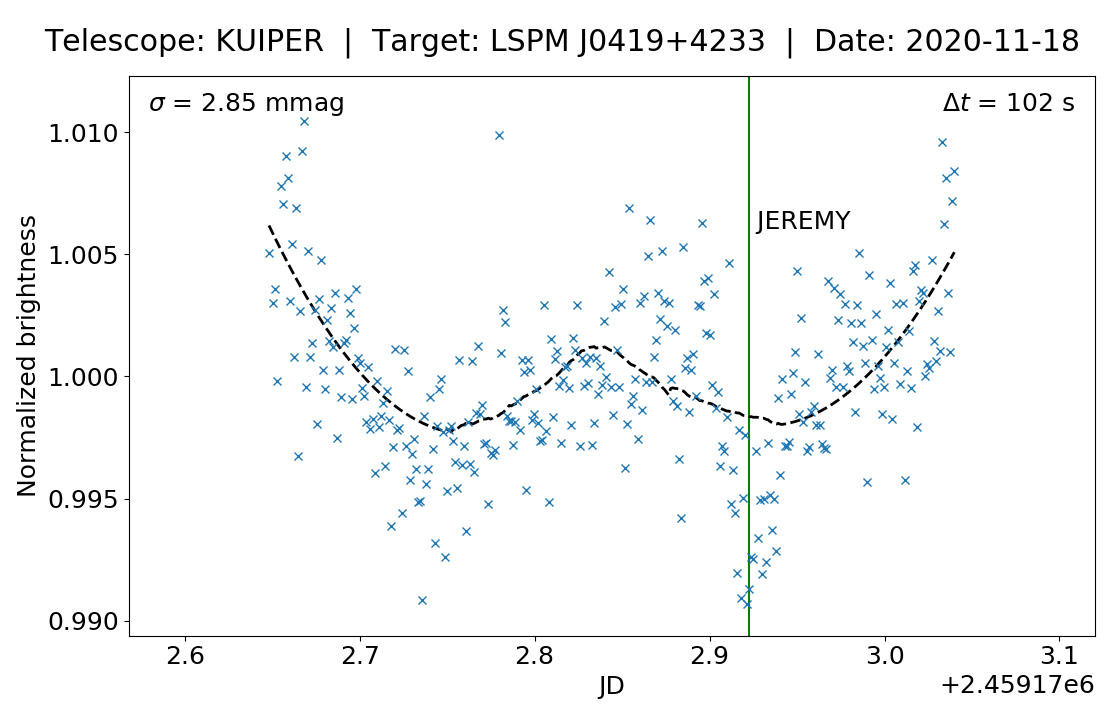
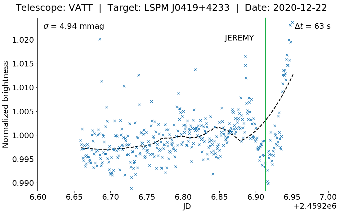
Figure 5: The first look at the non-detrended light curves from a simple reference star calibration of each potential transit event, before full detrending is done. The transit-like features are marked with green lines and the name of the Project EDEN member who analyzed the quick look data.

This star was also observed by TESS in Sector 19, and was found to have stellar variability with an amplitude of $\sim$1% on a 0.99 day period. Once that trend was removed, a low-confidence recurring event (SNR = 4.9, Signal Detection Efficiency (SDE)$\sim$6.5) was found with a period of 2.883 days and a transit depth of 0.7%. Notably, the ephemerides aligned with both the LOT and VATT detections – 12 orbits of separation with a period of 2.883 days between the two sets of data. However, additional observations from Lulin and Calar Alto ruled out additional transits during those observation windows, casting doubt on the veracity of the original transit observations.

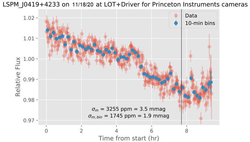
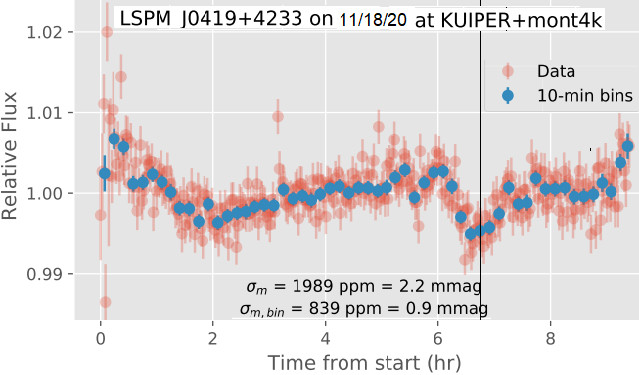
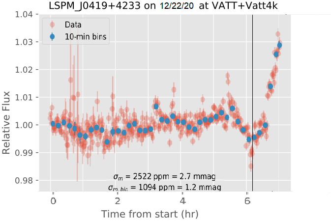
Figure 6: The three light curves (both full and 10-minute binned data) with errorbars for EIC 9 where we identified transit-like features (noted by black vertical lines in each panel). Top: Light curve from LOT on 18 Nov 2020 (UT); transit event originally identified (see Figure 5) centered at 7.8 hours (2459172.33 JD). Middle: Light curve from Kuiper on 18 Nov 2020 (UT) with transit event centered at 6.8 hours (2459172.91 JD). Bottom: Light curve from VATT on 22 Dec 2020 (UT); transit event centered at 6.1 hours (2459206.91 JD.)

Additional analysis of the light curves from the LOT and VATT events found both to be highly dependent on systematics, as the VATT event was at high airmass and the LOT event is cancelled out by the detrending procedure (compare the top panel of Figure 5 with the top panel of Figure 6 and the middle panel of Figure  7). The event in the Kuiper telescope light curve remained even through additional detrending. Previous observations from the Bok telescope in 2019 weren’t sensitive enough to rule out a transit of the given depth, but new data from the Calar Alto $1.23\,\mathrm{m}$ telescope in January 2021 ruled out the $\sim 2.883$-day period for the candidate (see Figure 7). Transit fitting of the signal from the Kuiper event put the period at 3.003 days with a 68% confidence interval of [1.735, 3.781] days. Based on our observing coverage of the target, we likely would have seen multiple transits of any planets within a 5-day period.

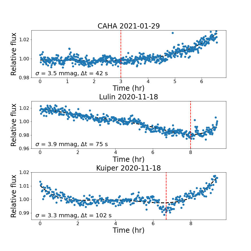
Figure 7: Additionally detrended light curves for EIC 9. Top: Follow-up light curve from Calar Alto in January 2021 with no transit feature near the expected mid-transit time from the TESS period (red dashed line). Middle: LOT light curve from November 2020 with the expected mid-transit time from TESS marked. No transit-like signal is visible. Bottom: Kuiper telescope light curve from November 2020, with the expected mid-transit time from a 2.886-day period. Here, a transit-like feature is visible.

Eventually, we determined that our effective phase coverage was providing diminishing returns on continued observations beyond $\sim$40 nights of data, so with no further transit signals we suspended the follow-up of this target and returned to the standard survey monitoring procedures. The event could be a transit, but we would likely have seen an additional transit in our observations unless the data quality was consistently poor. At this point the origin of the detected signal remains unexplained. It may have been caused by telluric contamination such as variable precipitable water vapor (see discussion in Sect. 3.3), which we shall estimate qualitatively here. Typical amounts of water vapor in the Santa Catalina Mountains of $2\text{\,}\mathrm{mm}$ have been measured (Warner, 1977). For a bandpass similar to GG495, this was estimated to cause a $\sim 3\text{\,}\mathrm{\char 37\relax}$ flux difference due to PWV for an M8 target star (Murray et al., 2020; Pedersen et al., 2023). According to these data, a PWV variation on the order of $1\text{\,}\mathrm{mm}$ would be consistent with a $1\text{\,}\mathrm{\char 37\relax}$-level flux change, making PWV variations a potentially viable source of the observed signal.

The TLS results from the full set of light curves of this target confirm our analysis of the potential signal. There was no strong event matching the period or any multiples of the expected transit from the TESS data, and the best transit model that TLS found had too short of a duration to be a physical transit of an exoplanet. In addition, none of the best-fit models from any of the precision cuts included the Kuiper event as a possible transit match.

7.3 Light curve analysis

Our observations were collected with seven telescopes located on three different continents. We developed a uniform observing protocol and data reduction and analysis approach that provided uniform final products, where differences are primarily due to the sensitivity of the instrument (a combination of the telescopes’ light-collecting area and the quantum efficiency of the detectors). Our data reduction and analysis approach was developed to simultaneously maximize sensitivity (finding many possible transit candidates and following up on them) and efficiency (observing many targets where follow-up monitoring requires a substantial amount of telescope time).

The EDEN survey’s sensitivity is demonstrated by the injection-and-retrieval tests we performed (see Section 4.2). Its efficiency is, perhaps counter-intuitively, reflected in the overall scarcity of possible detections: our sensitivity analysis shows that our observations can very efficiently detect short-period planets (P $<$1.5 d), even if they are relatively small (R${}_{p}<1.5R_{\oplus}$). Yet, during our survey of over 2,450 hours, we detected only one target with a potential single transit (see Section 7.2). The combination of high sensitivity and the very low number of false positives demonstrates high efficiency and reliability, as well as a robust approach for data reduction and analysis, which are particularly important for any targeted survey. In order to support future surveys, we commit to making the complete EDEN data analysis package available on a collaborative basis.

7.4 No planets detected

Project EDEN survey’s extensive dataset yielded multiple possible detections, but only EIC 9 was not identified immediately as a false positive. Further observations successfully eliminated it as a potential planet candidate, leaving no detected transit in our survey. Translating non-detections into constraints on the exoplanet demographics and occurrence rates is non-trivial, and requires a careful sensitivity analysis (see, e.g., Obermeier et al. 2016; Kunimoto & Matthews 2020; Sagear et al. 2020).

We performed injection-and-recovery based Monte Carlo sensitivity assessments for our targets and datasets, which mimic signals which would have been introduced by planets. In the initial EDEN survey paper (Gibbs et al., 2020), where our method was initially introduced, the efficiency was compared to (blind) injection and recovery by four team members. We found that the human team’s ability to identify randomly injected planets is comparable to the algorithmic identification. Therefore, the automatic injection-and-recovery sensitivity maps presented in Appendix A can be considered as a highly reliable assessment of the sensitivity of our dataset for each planet as a function of planet period and radius. The non-detection, in combination with the carefully characterized sensitivity limits, provides an important opportunity to place constraints on the occurrence rates of exoplanets around late M dwarfs.

7.5 Occurrence rates for different categories of planets

While we obtain a sensitivity of $\sim 30\%$ to transiting TRAPPIST-1b-like planets, the completeness with regard to these planets is low due to the small transit probabilities. Our Monte Carlo assessment of 10,000 mock surveys showed that even if every star had a TRAPPIST-1b-like planet or TRAPPIST-1 planetary system analog, we would detect planets either $15\text{\,}\mathrm{\char 37\relax}$ or $21\text{\,}\mathrm{\char 37\relax}$ of the time. In addition, Burn et al. (2021) found in planet formation models that occurrence rates of planets of all sizes drop from early M dwarfs to late M dwarfs. Based on a pebble accretion formation model, Mulders et al. (2021) suggest a drop in rocky planets toward the substellar boundary.

We can compare our results to other measurements from ultra-cool dwarf (UCD) surveys. The full TRAPPIST survey analysis (Lienhard et al., 2020) found that their expected number of detections, given every UCD had a TRAPPIST-1 b-like planet in the system, is 0.52. Thus, the detection of TRAPPIST-1 b in the survey sample of 40 UCDs implies a lower limit for the occurrence rate of TRAPPIST-1 b-like planets of 10% at 95% confidence. Sestovic & Demory (2020) examined the K2 light curves of 702 UCDs and were able to rule out TRAPPIST-1-like planetary systems around every UCD with 96% confidence, while Sagear et al. (2020) examined 827 K2 UCD light curves and found that the occurrence rate of TRAPPIST-1b analogs was limited to $<57\%$. The EDEN survey, with roughly half the number of targets as the full TRAPPIST survey analysis, shows a similar expected number of detections. Thus, even a targeted EDEN-like survey expanded out to >100 UCDs would still have at least a 50% chance of detecting no planets.

The case of giant planets is a separate consideration. Compared to FGK stars, M dwarfs host fewer giant planets (Endl et al., 2006; Johnson et al., 2010; Bonfils et al., 2013; Sabotta et al., 2021), which is in line with predictions of current planet formation models (e.g., Miguel & Ida, 2016; Liu et al., 2019; Mulders et al., 2021; Burn et al., 2021). The giant planet occurrence appears to decline linearly with decreasing stellar mass (Johnson et al., 2010; Ghezzi et al., 2018), although the continuation of this trend into the less explored late M dwarf regime has recently been questioned (Jordán et al., 2022; Schlecker et al., 2022). Under the optimistic assumption of a short-period ($P\sim 1$ day) giant planet around every star, $27\text{\,}\mathrm{\char 37\relax}$ of simulated EDEN surveys would still yield zero detections. Our data thus allows us to reject the hypothesis of one giant planet per star at a $73\text{\,}\mathrm{\char 37\relax}$ significance level. For ultra-short-period giant planets ($P=0.5$ days), our constraint on the occurrence rate at 95% confidence is $f_{\mathrm{large}}<$ $75\text{\,}\mathrm{\char 37\relax}$. We conclude that our non-detection is consistent with previous giant planet occurrence rates while not ruling out a moderate increase around late M dwarfs as recently suggested by Schlecker et al. (2022). A larger sample will be needed to provide stronger constraints. Assuming a comparable completeness for an extension of the survey, we find that a sample with at least $\sim 50$ stars is needed to exclude the hypothesis that every star hosts a (hot) giant planet with $95\text{\,}\mathrm{\char 37\relax}$ confidence.

8 Summary

The occurrence rate of TRAPPIST-like planets is not well constrained, as well as the occurrence rate of small planets around earlier M dwarfs and its dependency on spectral subtype (e.g., Hardegree-Ullman et al., 2019; Mulders et al., 2021). We have performed a northern-visible volume-complete survey out to 15 pc of the late (M7–L0) single and quiescent northern M dwarfs searching for transiting planets to test this hypothesis. The key findings of our study are as follows:

• We observed $>$ 25 hours for 22 target stars observable for $>$ 3 hours per night from the northern hemisphere and present high-precision light curves and data sets for all targets.

• We provided an improved planet-injection-based sensitivity analysis to remove low-sample-size noise.

• We carefully analyzed the data and found no convincing periodic planetary transit signals that held up to advanced scrutiny. We found one possible candidate in EDEN and TESS data, but further observations and analysis ruled out the origin of the signals as a repeating transit feature.

• The combination of high sensitivity and very low number of false positives demonstrated the high efficiency of our data analysis and planet identification process.

• We tested the fraction $f_{\mathrm{Trb}}$ of late M dwarfs hosting a TRAPPIST-1 b analog planet and $f_{\mathrm{Tr}}$ of a TRAPPIST-1 analog system. Given no detections in our survey, and the well-characterized sensitivity, we cannot exclude $f_{\mathrm{Trb}}<100\%$ (15% of surveys would detect a planet) nor an $f_{\mathrm{Tr}}<100\%$ (21% of surveys would detect a planet).

• Additionally, we tested the fraction $f_{\mathrm{large}}$ of late M dwarfs hosting a giant planet at a short orbital period $P=1.05$ days. We found that we cannot exclude $f_{\mathrm{large}}<100\%$ with 73% of simulated surveys detecting a planet. However, at 0.5 day orbital periods, we can constrain $f_{\mathrm{large}}<75\%$ at a 95% confidence level.

Our EDEN observations provide the most sensitive volume-complete photometric monitoring of late M dwarf stars to date and upper limits on the short-period planet population around TRAPPIST-1-like hosts. The observations presented here can guide future studies of the targeted systems and be used to test models of planet formation and evolution around the smallest stars.

The authors would like to thank Néstor Espinoza and José Pérez Angel Chávez for major contributions to the EDEN data processing pipeline, Allie Mousseau for creating the EDEN target catalog, Quentin J. Socia for observations at the Kuiper 61" and the VATT 1.8 m telescopes, and Roberto Gualandi for his technical assistance at the Cassini telescope. The results reported herein benefited from collaborations and/or information exchange within NASA’s Nexus for Exoplanet System Science (NExSS) research coordination network sponsored by NASAs Science Mission Directorate. This material is based upon work supported by the National Aeronautics and Space Administration under Agreements No. NNX15AD94G (Earths in Other Solar Systems, PI: Apai) and No. 80NSSC21K0593 (Alien Earths, PI: Apai). This research has made use of the NASA Exoplanet Archive, which is operated by the California Institute of Technology, under contract with the National Aeronautics and Space Administration under the Exoplanet Exploration Program. This research made use of Photutils, an Astropy package for detection and photometry of astronomical sources (Bradley et al., 2019). This research made use of the Cassini 1.52 m telescope, which is operated by INAF-OAS “Osservatorio di Astrofisica e Scienza dello Spazio” of Bologna in Loiano, Italy. This publication has made use of data collected at Lulin Observatory, partly supported by MoST grant 109-2112-M-008-001. We thank the mountain operations staff at University of Arizona, Mt. Lemmon Sky Center, Lulin Observatory, Calar Alto Observatory, Loiano Telescopes, Mt. Graham International Observatory, Vatican Advanced Technology Telescope, and Kitt Peak National Observatory. BVR thanks the Heising-Simons Foundation for support. LM acknowledges support from the “Fondi di Ricerca Scientifica d’Ateneo 2021” of the University of Rome “Tor Vergata”. TND acknowledges support provided by the Alexander von Humboldt Foundation in the framework of the Sofja Kovalevskaja Award endowed by the Federal Ministry of Education and Research. An allocation of computer time from the UA Research Computing High Performance Computing (HPC) at the University of Arizona is gratefully acknowledged.

Author contributions: JD coordinated the observations of the EDEN target list, performed the sensitivity analysis, and drafted the manuscript. DA, TH, PG, and W-PC are the Co-PIs who founded EDEN, defined its scope, goals, and methods, led proposals to fund the project and led the research groups performing the observations at the University of Arizona, the Max Planck Institute for Astronomy, the Vatican Observatory, and National Central University in Taiwan. LM led an additional major component out of Italy and the University of Rome “Tor Vergata”. DA, KKH-U, MS, KM, and NK provided important assistance for the light curve processing and sensitivity analysis and made major contributions to the manuscript as part of the EDEN “Tiger Team”. KKH-U assisted in EDEN Survey and Follow-up Observation Program target selection. DA, AG, BVR, and AB created the EDEN data processing pipeline and assisted with the sensitivity analysis. PG, RPB, AB, AG, JD, and MS observed with the VATT 1.8 m telescope. AB, AG, and JD observed with the Bok 2.3 m telescope. AB, JD, KKH-U, and MS observed with the Kuiper 61" telescope. MS and NK coordinated the observing program at MPIA. MS, KM, NK, SB-S, Re.Bu., TND, LF, RF, GP, SS, and JS observed with the Calar Alto 1.23 m telescope. LM and IB observed with the Loiano Cassini 152 cm telescope. C-CN and A-LT coordinated the observing program at NCU. H-CL, C-SL, H-YH, and W-JH observed with the Lulin One-meter Telescope. W-HI and C-LL provided Lulin light curve analysis. Ri.Ba. processed light curves and assisted with Kuiper 61" observations.

, Wōtan (Hippke et al., 2019)

Appendix A Sensitivity Maps

Here in Figures 8-10 we show the sensitivity maps for the volume-complete 22 EDEN survey targets we observed. The targets that were found to be binaries after the beginning of observations are shown separately in Figure 11 at the end.

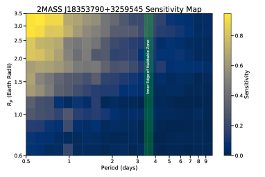
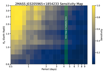
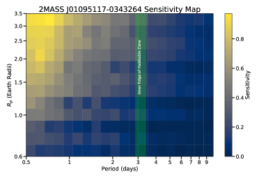
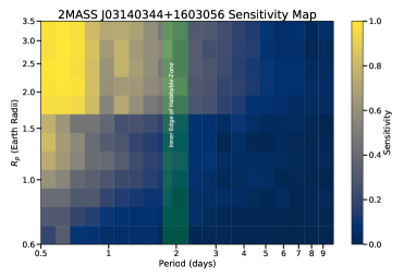
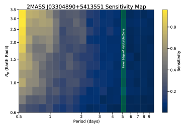
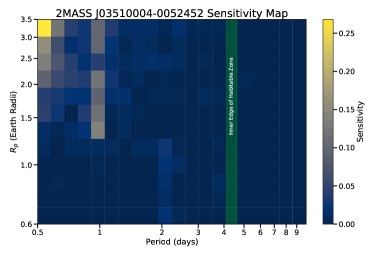
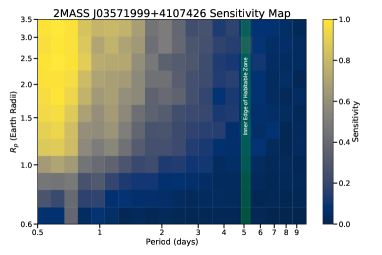
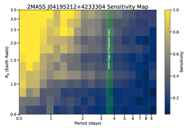
Figure 8: Sensitivity maps for EIC 1, 2, 4, 5, 6, 7, 8, 9

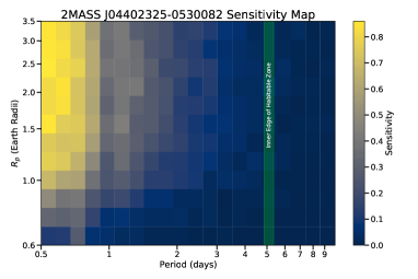
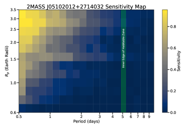
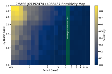
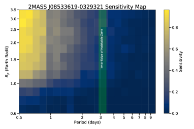
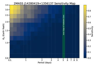
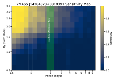
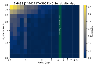
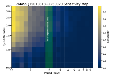
Figure 9: Sensitivity maps for EIC 11, 12, 13, 15, 16, 17, 18, 19

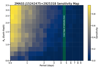
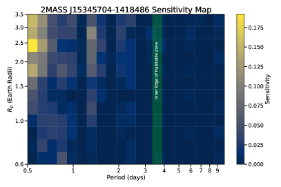
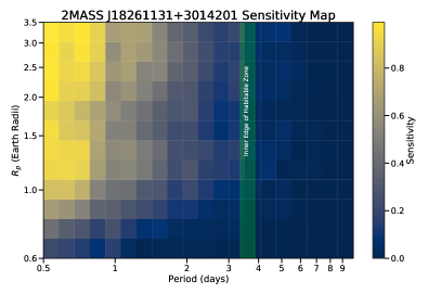
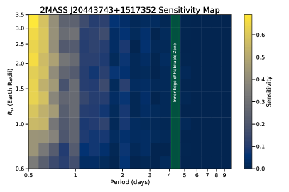
Figure 10: Sensitivity maps for EIC 20, 21, 22, 23

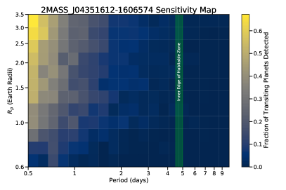
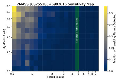
Figure 11: Sensitivity maps for the targets found to be binary stars, EIC 10 and 14

Appendix B Other EDEN Observations

Here we show a table of the other observations taken by Project EDEN on targets at distances of 15-37 pc, earlier spectral types from M2-M6, and for targeted follow-up observations with the TESS Follow-up Observing Program (TFOP).

Table 3: EDEN Observations of non-survey and non-follow-up targets

2MASS ID	Distance (pc)	Spectral Type	Hours Observed
Observed Targets from 15-21 pc
J00194579+5213179	19.96	M9	314.6
J01242326+6819312	20.78	M7V	124.3
J01400263+2701505	18.99	M8.5V	25.3
J03395284+2457273	19.27	M7.7V	18.1
J05153094+5911184	15.22	M7V	122.0
J07140394+3702459	15.61	M8	294.1
J07410681+1738459	15.67	M7V	10.0
J08072607+3213101	18.88	M8	101.2
J09032096+0540145	17.48	M7V	111.3
J10163470+2751497	17.24	M8V	276.5
J10554733+0808427	18.75	M9V	165.7
J13564148+4342587	19.98	M8V	189.2
J14032232+3007547	19.81	M9V	4.5
J15512179+2931062	18.48	M7	48.1
J22254853+6421479	16.50	M9.5	12.2
Observed non-EDEN Survey Targets
J00192626+4614078	38.34	M8	87.1
J02170993+3526330∗	10.37	M7V	235.6
J02530084+1652532	3.83	dM6	5.9
J04351612-16065742	10.604	M8Ve	32.9
J05402570+2448090∗	10.25	M7V	51.0
J06083043+4902063	37.52	M5V	0.7
J07464256+2000321	12.36	L0+L2	1.4
J07590587+1523294	29.45	M2V	3.4
J08022287+0320196	27.39	M4V	20.9
J08402975+1824091∗	13.56	M6V	6.3
J10022184+4805209	14.96	M1V	21.0
J10471382+4026493	25.73	M8	3.2
J10562886+0700527∗	2.42	M6	103.8
J11224274+3755484	17.69	M6V	1.0
J11505787+4822394	7.66	M4.5Ve	16.4
J12003292+2048513	24.62	M8V	1.8
J12030930+1701230	36.88	M6V	1.4
J12555681+5055219	21.56	M4V	24.4
J13481341+2336486	11.88	M5V	3.5
J16005083+4019441	21.14	M3	0.6
J17151894+0457496	14.65	M4.5V	68.4
J17351296+2634475	15.55	M7.5+L0	91.4
J18393308+2952164	12.17	M6.5Ve	73.0
J18432213+4040209∗	14.40	M7.5V	171.2
J20450403+4429562	12.05	M2V	15.7
J23415498+4410407	3.16	M5V	24.9

Notes: ^∗: Eruptive or cataclysmic variable star. ² Unresolved binary star EIC 10.

Table 4: EDEN Observations of non-survey targets

TIC ID	Distance (pc)	Spectral Type	Hours Observed
Observed TESS Follow-up Observation Program (TFOP) Targets
8348911	51.60	$\sim$M4V	3.6
9032367	586.30	$\sim$K3V	4.5
29918916	354.96	G2IV[1]	7.8
43064903	24.54	M4.5	5.4
66783360	254.19	$\sim$F5.5V	6.3
98720702	99.15	M3V	3.2
104208182	142.04	$\sim$K7V	7.1
142748283	48.48	$\sim$M4V	4.6
144401492	119.24	K0III	2.9
175194958	190.21	M1V	0.6
175241416	13.55	M6V	4.8
180652891	314.98	Am	1.7
181804572	26.49	M6V	25.7
198212955	109.52	$\sim$K6V	5.1
212957629	55.60	$\sim$M5V	3.4
232608943	216.06	$\sim$K1V	6.0
233211762	152.00	$\sim$K7V	3.8
235678745	41.92	$\sim$M1.5V	5.3
233602827	99.42	$\sim$M0V	16.1
237808867	967.77	G0III[1]	2.4
240968774	37.48	$\sim$M1V	1.9
243185500	24.76	$\sim$M3V	37.8
267561446	110.60	$\sim$M0V	3.2
269701147	53.69	G0	0.9
278892590+	12.43	M7.5e	11.0
284441182	51.74	$\sim$M1V	3.5
288185138	233.77	$\sim$F8V	0.9
357972447	256.25	$\sim$F1V	1.8
363445338	245.53	K7V	4.7
368287008	47.32	$\sim$M3.5V	4.4
377909730	440.12	$\sim$K3V	4.1
399860444	216.67	G0V	5.9
408203452†	N/A	N/A	12.1
408203470	74.80	$\sim$M3V	8.2
435931205	326.41	G8IV[1]	37.1
436584697	52.10	$\sim$M3V	3.2
439867639	48.65	$\sim$M4V	2.7
441738827	114.93	$\sim$M1.5V	6.0

Notes: ^†: Star had zero/negative parallax in Gaia and no stellar parameters in TIC v8.1. ⁺: TRAPPIST-1. Spectral type taken from SIMBAD unless otherwise noted here. $\sim$ indicates value gathered from TIC v8.1 temperature and mass/radius measurements and utilizing the main sequence relations from Pecaut & Mamajek (2013). [1]: No spectral type in SIMBAD, TIC v8.1 temperature and radius measurements are very similar to stars of these types.

References

- Agol et al. (2021) Agol, E., Dorn, C., Grimm, S. L., et al. 2021, \psj, 2, 1, doi: 10.3847/PSJ/abd022
- Apai et al. (2019) Apai, D., Milster, T. D., Kim, D. W., et al. 2019, AJ, 158, 83, doi: 10.3847/1538-3881/ab2631
- Apai et al. (2018) Apai, D., Ciesla, F., Mulders, G. D., et al. 2018, arXiv e-prints, arXiv:1803.08682. https://arxiv.org/abs/1803.08682
- Bailer-Jones & Lamm (2003) Bailer-Jones, C., & Lamm, M. 2003, Monthly Notices of the Royal Astronomical Society, 339, 477, doi: 10.1046/j.1365-8711.2003.06189.x
- Bakos et al. (2002) Bakos, G. Á., Lázár, J., Papp, I., Sári, P., & Green, E. M. 2002, PASP, 114, 974, doi: 10.1086/342382
- Bardalez Gagliuffi et al. (2014) Bardalez Gagliuffi, D. C., Burgasser, A. J., Gelino, C. R., et al. 2014, ApJ, 794, 143, doi: 10.1088/0004-637X/794/2/143
- Berger et al. (2020) Berger, T. A., Huber, D., van Saders, J. L., et al. 2020, AJ, 159, 280, doi: 10.3847/1538-3881/159/6/280
- Berta et al. (2013) Berta, Z. K., Irwin, J., & Charbonneau, D. 2013, The Astrophysical Journal, 775, 91, doi: 10.1088/0004-637X/775/2/91
- Berta et al. (2012) Berta, Z. K., Irwin, J., Charbonneau, D., Burke, C. J., & Falco, E. E. 2012, The Astronomical Journal, 144, 145, doi: 10.1088/0004-6256/144/5/145
- Bitsch et al. (2021) Bitsch, B., Raymond, S. N., Buchhave, L. A., et al. 2021, Astronomy & Astrophysics, 649, L5, doi: 10.1051/0004-6361/202140793
- Blake et al. (2008) Blake, C. H., Bloom, J. S., Latham, D. W., et al. 2008, Publications of the Astronomical Society of the Pacific, 120, 860, doi: 10.1086/590506
- Bonfils et al. (2013) Bonfils, X., Delfosse, X., Udry, S., et al. 2013, Astronomy & Astrophysics, 549, A109, doi: 10.1051/0004-6361/201014704
- Borucki et al. (2010) Borucki, W. J., Koch, D., Basri, G., et al. 2010, Science, 327, 977, doi: 10.1126/science.1185402
- Bradley et al. (2019) Bradley, L., Sipőcz, B., Robitaille, T., et al. 2019, astropy/photutils: v0.7.2, v0.7.2, Zenodo, doi: 10.5281/zenodo.3568287
- Buchner et al. (2014) Buchner, J., Georgakakis, A., Nandra, K., et al. 2014, A&A, 564, A125, doi: 10.1051/0004-6361/201322971
- Burn et al. (2021) Burn, R., Schlecker, M., Mordasini, C., et al. 2021, Astronomy & Astrophysics, 656, A72, doi: 10.1051/0004-6361/202140390
- Claret (1998) Claret, A. 1998, A&A, 335, 647
- Clark et al. (2022a) Clark, C. A., van Belle, G. T., Ciardi, D. R., et al. 2022a, AJ, 163, 232, doi: 10.3847/1538-3881/ac6101
- Clark et al. (2022b) Clark, C. A., van Belle, G. T., Horch, E. P., et al. 2022b, arXiv e-prints, arXiv:2205.12922. https://arxiv.org/abs/2205.12922
- Delrez et al. (2018) Delrez, L., Gillon, M., Queloz, D., et al. 2018, in Society of Photo-Optical Instrumentation Engineers (SPIE) Conference Series, Vol. 10700, Ground-based and Airborne Telescopes VII, ed. H. K. Marshall & J. Spyromilio, 107001I, doi: 10.1117/12.2312475
- Deshpande et al. (2012) Deshpande, R., Martín, E. L., Montgomery, M. M., et al. 2012, AJ, 144, 99, doi: 10.1088/0004-6256/144/4/99
- Dressing & Charbonneau (2015) Dressing, C. D., & Charbonneau, D. 2015, ApJ, 807, 45, doi: 10.1088/0004-637X/807/1/45
- El-Badry et al. (2021) El-Badry, K., Rix, H.-W., & Heintz, T. M. 2021, MNRAS, 506, 2269, doi: 10.1093/mnras/stab323
- Endl et al. (2006) Endl, M., Cochran, W. D., Kurster, M., et al. 2006, The Astrophysical Journal, 649, 436, doi: 10.1086/506465
- Fabrycky et al. (2014) Fabrycky, D. C., Lissauer, J. J., Ragozzine, D., et al. 2014, ApJ, 790, 146, doi: 10.1088/0004-637X/790/2/146
- Faherty et al. (2009) Faherty, J. K., Burgasser, A. J., Cruz, K. L., et al. 2009, AJ, 137, 1, doi: 10.1088/0004-6256/137/1/1
- Furlan et al. (2017) Furlan, E., Ciardi, D. R., Everett, M. E., et al. 2017, AJ, 153, 71, doi: 10.3847/1538-3881/153/2/71
- Gaia Collaboration et al. (2022a) Gaia Collaboration, Vallenari, A., Brown, A., Prusti, T., & et al. 2022a, Astronomy & Astrophysics
- Gaia Collaboration et al. (2021) Gaia Collaboration, Smart, R. L., Sarro, L. M., et al. 2021, A&A, 649, A6, doi: 10.1051/0004-6361/202039498
- Gaia Collaboration et al. (2022b) Gaia Collaboration, Arenou, F., Babusiaux, C., et al. 2022b, arXiv e-prints, arXiv:2206.05595. https://arxiv.org/abs/2206.05595
- Gaudi et al. (2020) Gaudi, B. S., Seager, S., Mennesson, B., et al. 2020, arXiv e-prints, arXiv:2001.06683. https://arxiv.org/abs/2001.06683
- Ghezzi et al. (2018) Ghezzi, L., Montet, B. T., & Johnson, J. A. 2018, The Astrophysical Journal, 860, 109, doi: 10.3847/1538-4357/aac37c
- Gibbs et al. (2020) Gibbs, A., Bixel, A., Rackham, B. V., et al. 2020, AJ, 159, 169, doi: 10.3847/1538-3881/ab7926
- Gillon et al. (2016) Gillon, M., Jehin, E., Lederer, S. M., et al. 2016, Nature, 533, 221, doi: 10.1038/nature17448
- Gillon et al. (2017) Gillon, M., Triaud, A. H. M. J., Demory, B.-O., et al. 2017, Nature, 542, 456, doi: 10.1038/nature21360
- Gizis et al. (2000) Gizis, J. E., Monet, D. G., Reid, I. N., et al. 2000, AJ, 120, 1085, doi: 10.1086/301456
- Hardegree-Ullman et al. (2019) Hardegree-Ullman, K. K., Cushing, M. C., Muirhead, P. S., & Christiansen, J. L. 2019, AJ, 158, 75, doi: 10.3847/1538-3881/ab21d2
- Hardegree-Ullman et al. (2020) Hardegree-Ullman, K. K., Zink, J. K., Christiansen, J. L., et al. 2020, ApJS, 247, 28, doi: 10.3847/1538-4365/ab7230
- Harris et al. (2020) Harris, C. R., Millman, K. J., van der Walt, S. J., et al. 2020, Nature, 585, 357, doi: 10.1038/s41586-020-2649-2
- Henry et al. (2006) Henry, T. J., Jao, W.-C., Subasavage, J. P., et al. 2006, AJ, 132, 2360, doi: 10.1086/508233
- Henry et al. (2018) Henry, T. J., Jao, W.-C., Winters, J. G., et al. 2018, AJ, 155, 265, doi: 10.3847/1538-3881/aac262
- Hippke et al. (2019) Hippke, M., David, T. J., Mulders, G. D., & Heller, R. 2019, AJ, 158, 143, doi: 10.3847/1538-3881/ab3984
- Hippke & Heller (2019) Hippke, M., & Heller, R. 2019, TLS: Transit Least Squares. http://ascl.net/1910.007
- Huang et al. (2020) Huang, L. C., Ip, W. H., Lin, C. L., et al. 2020, ApJ, 892, 58, doi: 10.3847/1538-4357/ab774a
- Ida & Lin (2004) Ida, S., & Lin, D. N. C. 2004, The Astrophysical Journal, 616, 567, doi: 10.1086/424830
- Irwin et al. (2009) Irwin, J., Charbonneau, D., Nutzman, P., & Falco, E. 2009, in Transiting Planets, ed. F. Pont, D. Sasselov, & M. J. Holman, Vol. 253, 37–43, doi: 10.1017/S1743921308026215
- Izidoro et al. (2021) Izidoro, A., Bitsch, B., Raymond, S. N., et al. 2021, Astronomy & Astrophysics, 650, A152, doi: 10.1051/0004-6361/201935336
- Johnson et al. (2010) Johnson, J. A., Aller, K. M., Howard, A. W., & Crepp, J. R. 2010, Publications of the Astronomical Society of the Pacific, 122, 905, doi: 10.1086/655775
- Jordán et al. (2022) Jordán, A., Hartman, J. D., Bayliss, D., et al. 2022, The Astronomical Journal, 163, 125, doi: 10.3847/1538-3881/ac4a77
- Kasper et al. (2007) Kasper, M., Apai, D., Janson, M., & Brandner, W. 2007, A&A, 472, 321, doi: 10.1051/0004-6361:20077646
- Kiman et al. (2019) Kiman, R., Schmidt, S. J., Angus, R., et al. 2019, AJ, 157, 231, doi: 10.3847/1538-3881/ab1753
- Kimura & Ikoma (2022) Kimura, T., & Ikoma, M. 2022, Nature Astronomy, 1, doi: 10.1038/s41550-022-01781-1
- Kirkpatrick et al. (2011) Kirkpatrick, J. D., Cushing, M. C., Gelino, C. R., et al. 2011, ApJS, 197, 19, doi: 10.1088/0067-0049/197/2/19
- Kopparapu et al. (2013) Kopparapu, R. K., Ramirez, R., Kasting, J. F., et al. 2013, ApJ, 765, 131, doi: 10.1088/0004-637X/765/2/131
- Kreidberg (2015) Kreidberg, L. 2015, PASP, 127, 1161, doi: 10.1086/683602
- Kunimoto & Matthews (2020) Kunimoto, M., & Matthews, J. M. 2020, AJ, 159, 248, doi: 10.3847/1538-3881/ab88b0
- Lang et al. (2010) Lang, D., Hogg, D. W., Mierle, K., Blanton, M., & Roweis, S. 2010, AJ, 139, 1782, doi: 10.1088/0004-6256/139/5/1782
- Lépine et al. (2002) Lépine, S., Rich, R. M., Neill, J. D., Caulet, A., & Shara, M. M. 2002, ApJ, 581, L47, doi: 10.1086/345943
- Lienhard et al. (2020) Lienhard, F., Queloz, D., Gillon, M., et al. 2020, MNRAS, 497, 3790, doi: 10.1093/mnras/staa2054
- Lin et al. (2021) Lin, C.-L., Chen, W.-P., Ip, W.-H., et al. 2021, AJ, 162, 11, doi: 10.3847/1538-3881/abf933
- Liu et al. (2019) Liu, B., Lambrechts, M., Johansen, A., & Liu, F. 2019, Astronomy & Astrophysics, 632, A7, doi: 10.1051/0004-6361/201936309
- Luger et al. (2017) Luger, R., Lustig-Yaeger, J., & Agol, E. 2017, ApJ, 851, 94, doi: 10.3847/1538-4357/aa9c43
- Meier Valdés et al. (2021) Meier Valdés, E. A., Morris, B. M., & Demory, B. O. 2021, A&A, 649, A132, doi: 10.1051/0004-6361/202039629
- Miguel & Ida (2016) Miguel, Y., & Ida, S. 2016, Icarus, 266, 1, doi: 10.1016/j.icarus.2015.10.030
- Moe & Kratter (2021) Moe, M., & Kratter, K. M. 2021, Monthly Notices of the Royal Astronomical Society, 507, 3593, doi: 10.1093/mnras/stab2328
- Mordasini et al. (2009) Mordasini, C., Alibert, Y., Benz, W., & Naef, D. 2009, Astronomy and Astrophysics, 501, 1161, doi: 10.1051/0004-6361/200810697
- Mulders et al. (2021) Mulders, G. D., Drążkowska, J., van der Marel, N., Ciesla, F. J., & Pascucci, I. 2021, ApJ, 920, L1, doi: 10.3847/2041-8213/ac2947
- Mulders et al. (2015) Mulders, G. D., Pascucci, I., & Apai, D. 2015, ApJ, 798, 112, doi: 10.1088/0004-637X/798/2/112
- Mulders et al. (2018) Mulders, G. D., Pascucci, I., Apai, D., & Ciesla, F. J. 2018, AJ, 156, 24, doi: 10.3847/1538-3881/aac5ea
- Murray et al. (2020) Murray, C. A., Delrez, L., Pedersen, P. P., et al. 2020, Monthly Notices of the Royal Astronomical Society, 495, 2446, doi: 10.1093/mnras/staa1283
- Murray et al. (2022) Murray, C. A., Queloz, D., Gillon, M., et al. 2022, MNRAS, 513, 2615, doi: 10.1093/mnras/stac1078
- Ndugu et al. (2018) Ndugu, N., Bitsch, B., & Jurua, E. 2018, Monthly Notices of the Royal Astronomical Society, 474, 886, doi: 10.1093/mnras/stx2815
- Newton et al. (2014) Newton, E. R., Charbonneau, D., Irwin, J., et al. 2014, AJ, 147, 20, doi: 10.1088/0004-6256/147/1/20
- Nutzman & Charbonneau (2008) Nutzman, P., & Charbonneau, D. 2008, Publications of the Astronomical Society of the Pacific, 120, 317, doi: 10.1086/533420
- Obermeier et al. (2016) Obermeier, C., Koppenhoefer, J., Saglia, R. P., et al. 2016, Astronomy & Astrophysics, 587, A49, doi: 10.1051/0004-6361/201527633
- Offner et al. (2022) Offner, S. S. R., Moe, M., Kratter, K. M., et al. 2022, The Origin and Evolution of Multiple Star Systems
- Pecaut & Mamajek (2013) Pecaut, M. J., & Mamajek, E. E. 2013, ApJS, 208, 9, doi: 10.1088/0067-0049/208/1/9
- Pedersen et al. (2023) Pedersen, P. P., Murray, C. A., Queloz, D., et al. 2023, Monthly Notices of the Royal Astronomical Society, 518, 2661, doi: 10.1093/mnras/stac3154
- Pepper et al. (2003) Pepper, J., Gould, A., & Depoy, D. L. 2003, Acta Astron., 53, 213. https://arxiv.org/abs/astro-ph/0208042
- Pinamonti et al. (2022) Pinamonti, M., Sozzetti, A., Maldonado, J., et al. 2022, arXiv e-prints, arXiv:2203.04648. https://arxiv.org/abs/2203.04648
- Price-Whelan et al. (2018) Price-Whelan, A., Crawford, S., Sipocz, B., et al. 2018, Astropy/Astropy-V2.0-Paper: Final Draft, final draft, Zenodo, doi: 10.5281/zenodo.1211397
- Quanz (2019) Quanz, S. 2019, in EPSC-DPS Joint Meeting 2019, Vol. 2019, EPSC–DPS2019–327
- Reiners & Basri (2009) Reiners, A., & Basri, G. 2009, ApJ, 705, 1416, doi: 10.1088/0004-637X/705/2/1416
- Reiners et al. (2018) Reiners, A., Zechmeister, M., Caballero, J. A., et al. 2018, A&A, 612, A49, doi: 10.1051/0004-6361/201732054
- Reylé (2018) Reylé, C. 2018, A&A, 619, L8, doi: 10.1051/0004-6361/201834082
- Ricker et al. (2015) Ricker, G. R., Winn, J. N., Vanderspek, R., et al. 2015, Journal of Astronomical Telescopes, Instruments, and Systems, 1, 014003, doi: 10.1117/1.JATIS.1.1.014003
- Sabotta et al. (2021) Sabotta, S., Schlecker, M., Chaturvedi, P., et al. 2021, Astronomy & Astrophysics, 653, A114, doi: 10.1051/0004-6361/202140968
- Sagear et al. (2020) Sagear, S. A., Skinner, J. N., & Muirhead, P. S. 2020, The Astronomical Journal, 160, 19, doi: 10.3847/1538-3881/ab9224
- Salama et al. (2021) Salama, M., Ou, J., Baranec, C., et al. 2021, AJ, 162, 102, doi: 10.3847/1538-3881/ac0445
- Salama et al. (2022) Salama, M., Ziegler, C., Baranec, C., et al. 2022, AJ, 163, 200, doi: 10.3847/1538-3881/ac53fc
- Schlecker et al. (2021a) Schlecker, M., Mordasini, C., Emsenhuber, A., et al. 2021a, Astronomy & Astrophysics, 656, A71, doi: 10.1051/0004-6361/202038554
- Schlecker et al. (2021b) Schlecker, M., Pham, D., Burn, R., et al. 2021b, Astronomy & Astrophysics, 656, A73, doi: 10.1051/0004-6361/202140551
- Schlecker et al. (2022) Schlecker, M., Burn, R., Sabotta, S., et al. 2022, RV-detected Planets around M Dwarfs: Challenges for Core Accretion Models, doi: 10.48550/arXiv.2205.12971
- Sebastian et al. (2021) Sebastian, D., Gillon, M., Ducrot, E., et al. 2021, A&A, 645, A100, doi: 10.1051/0004-6361/202038827
- Sestovic & Demory (2020) Sestovic, M., & Demory, B.-O. 2020, A&A, 641, A170, doi: 10.1051/0004-6361/202037732
- Shan et al. (2015) Shan, Y., Johnson, J. A., & Morton, T. D. 2015, ApJ, 813, 75, doi: 10.1088/0004-637X/813/1/75
- Skrutskie et al. (2006) Skrutskie, M. F., Cutri, R. M., Stiening, R., et al. 2006, AJ, 131, 1163, doi: 10.1086/498708
- Smart et al. (2017) Smart, R. L., Marocco, F., Caballero, J. A., et al. 2017, MNRAS, 469, 401, doi: 10.1093/mnras/stx800
- Southworth et al. (2009) Southworth, J., Hinse, T. C., Jørgensen, U. G., et al. 2009, MNRAS, 396, 1023, doi: 10.1111/j.1365-2966.2009.14767.x
- Susemiehl & Meyer (2022) Susemiehl, N., & Meyer, M. R. 2022, A&A, 657, A48, doi: 10.1051/0004-6361/202038582
- Tamburo et al. (2022) Tamburo, P., Muirhead, P. S., McCarthy, A. M., et al. 2022, AJ, 163, 253, doi: 10.3847/1538-3881/ac64aa
- The LUVOIR Team (2019) The LUVOIR Team. 2019, arXiv e-prints, arXiv:1912.06219. https://arxiv.org/abs/1912.06219
- Thommes et al. (2008) Thommes, E. W., Matsumura, S., & Rasio, F. A. 2008, Science, 321, 814, doi: 10.1126/science.1159723
- Virtanen et al. (2020) Virtanen, P., Gommers, R., Oliphant, T. E., et al. 2020, Nature Methods, 17, 261, doi: 10.1038/s41592-019-0686-2
- Vrijmoet et al. (2020) Vrijmoet, E. H., Henry, T. J., Jao, W.-C., & Dieterich, S. B. 2020, AJ, 160, 215, doi: 10.3847/1538-3881/abb4e9
- Warner (1977) Warner, J. W. 1977, PASP, 89, 724, doi: 10.1086/130217
- Wells et al. (2021) Wells, R. D., Rackham, B. V., Schanche, N., et al. 2021, A&A, 653, A97, doi: 10.1051/0004-6361/202141277
- Winters et al. (2019) Winters, J. G., Henry, T. J., Jao, W.-C., et al. 2019, AJ, 157, 216, doi: 10.3847/1538-3881/ab05dc