Robustness to Spurious Correlations Improves Semantic Out-of-Distribution Detection

Abstract

Methods which utilize the outputs or feature representations of predictive models have emerged as promising approaches for out-of-distribution (ood) detection of image inputs. However, these methods struggle to detect ood inputs that share nuisance values (e.g. background) with in-distribution inputs. The detection of shared-nuisance out-of-distribution (sn-ood) inputs is particularly relevant in real-world applications, as anomalies and in-distribution inputs tend to be captured in the same settings during deployment. In this work, we provide a possible explanation for sn-ood detection failures and propose nuisance-aware ood detection to address them. Nuisance-aware ood detection substitutes a classifier trained via Empirical Risk Minimization (erm) and cross-entropy loss with one that 1. is trained under a distribution where the nuisance-label relationship is broken and 2. yields representations that are independent of the nuisance under this distribution, both marginally and conditioned on the label. We can train a classifier to achieve these objectives using Nuisance-Randomized Distillation (nurd), an algorithm developed for ood generalization under spurious correlations. Output- and feature-based nuisance-aware ood detection perform substantially better than their original counterparts, succeeding even when detection based on domain generalization algorithms fails to improve performance.

1 Introduction

Out-of-distribution (ood) detection is the task of identifying inputs that fall outside the training distribution. A natural approach is to estimate the training distribution via a generative model and flag low-density inputs as ood (Bishop 1994), but such an approach has been shown to perform worse than random chance on several image tasks (Nalisnick et al. 2019), likely due to model estimation error (Zhang, Goldstein, and Ranganath 2021). Instead, many detection methods utilize either the outputs or feature representations of a learned classifier, yielding results much better than those of deep generative models on many tasks (Lee et al. 2018; Salehi et al. 2021)

However, classifier-based ood detection has been shown to struggle when ood and in-distribution (id) inputs share the same values of a nuisance variable that is of no inherent interest to the semantic task, e.g. the background of an image (Ming, Yin, and Li 2022). We call such ood inputs shared-nuisance ood (sn-ood) examples. For example, in the Waterbirds dataset (Sagawa et al. 2020), the image background (water or land) is a nuisance in the task of classifying bird type (waterbird vs. landbird), and an image of a boat on water is an sn-ood input, given the familiar background nuisance value but novel object label. Detection of sn-ood images is worse than detection of ood images with novel nuisance values. Moreover, the stronger the correlation between the nuisance and label in the training distribution, the worse the detection of sn-ood inputs. Even when classifiers are trained via domain generalization algorithms intended for generalizing to new test domains, detection does not improve (Ming, Yin, and Li 2022).

This failure mode is far from a rare edge case, given the relevance of sn-ood inputs in real-world applications. While an instance can be ood with respect to labels (e.g. new object) or nuisances (e.g. new background), in most cases, the goal is semantic ood detection, or detecting out-of-scope inputs (Yang et al. 2021). For instance, manufacturing plants are interested in product defects on the factory floor, not working products in new settings.

In this work, we introduce nuisance-aware ood detection to address sn-ood detection failures detection. Our contributions:

1. We present explanations for output- and feature-based sn-ood detection failures based on the role of nuisances in the learned predictor and its representations (Section 3).

2. We illustrate why models that are robust to spurious correlations can yield better output-based sn-ood detection and identify a predictor with such robustness guarantees to use for ood detection (Section 4).

3. We explain why removing nuisance information from representations can improve feature-based sn-ood detection and propose a joint independence constraint to achieve this end (Section 4).

4. We describe how domain generalization algorithms can fail to improve sn-ood detection, providing insight into the empirical failures seen previously (Section 5).

5. We show empirically that nuisance-aware ood detection improves detection on sn-ood inputs while maintaining performance on non-sn-ood ones (Section 7).

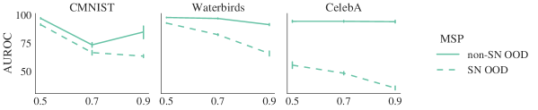
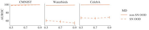
Figure 1: Output- and feature-based detection methods perform worse on shared-nuisance out-of-distribution inputs (see Section 7 for task details). The performance of output-based shared-nuisance ood detection (MSP, top) degrades under increasing spurious correlation strength (x-axis). Figure 7 shows the same trend for other output-based methods. The performance of feature-based ood detection (MD, bottom) is more stable but poor. See Appendix for plots of other common ood detection methods, which follow a similar trend.

2 Background

Most methods which employ predictive models for out-of-distribution detection can be categorized as either output-based or feature-based. Output-based methods utilize some function of the logits as an anomaly, while feature-based methods utilize internal representations of the learned model.

Output-based Out-of-distribution Detection

Let $f:\mathbb{R}^{D}\rightarrow\mathbb{R}^{K}$ be the learned function mapping an $D$-dimensional input to $K$ logits for the $K$ id classes. Output-based methods utilize some function of the logits $f(\textbf{x})\in\mathbb{R}^{K}$ as an anomaly score. Letting $\sigma$ denote the softmax function, relevant methods include maximum softmax probability (msp) or $\max_{k}\sigma(f(\textbf{x}))_{k}$ (Hendrycks and Gimpel 2017), max logit or $\max_{k}f_{k}(\textbf{x})$ (Hendrycks et al. 2022), the energy score or $\scalebox{0.75}[1.0]{$-$}\log\sum_{k}\exp{f_{k}(\textbf{x})}$ (Liu et al. 2020), and out-of-distribution detector for neural networks (odin) or $\max_{k}\sigma(f_{k}(\widetilde{\textbf{x}})/T)$, where $T$ is a learned temperature parameter and $\widetilde{\textbf{x}}$ is an input perturbed in the direction of the gradient of the maximum softmax probability (Liang, Li, and Srikant 2018).

Feature-based Out-of-distribution Detection

Feature-based methods utilize internal representations of the learned classifier. Following prior work (Kamoi and Kobayashi 2020; Ren et al. 2021; Fort, Ren, and Lakshminarayanan 2021), we consider the penultimate feature activations $r(\textbf{x})$. The most widely used feature-based method is the Mahalanobis distance (md) (Lee et al. 2018), which models the feature representations of in-distribution data as class-conditional Gaussians with means $\mu_{k}$ and shared covariance $\Sigma$. At test time, the anomaly score is the minimum Mahalanobis distance from a new input’s feature representations to each of these class distributions, $\min_{k}\sqrt{(r(\textbf{x})-\mu_{k})\Sigma^{-1}(r(\textbf{x})-\mu_{k})^{\top}}=\max_{k}p(r(\textbf{x})|\textbf{y}=k)$. Assuming minimal overlap in probability mass across each class-conditional Gaussian (e.g. tight and separated clusters), this method can approximate detection based on density estimation on the representations: $\max_{k}p(r(\textbf{x})|\textbf{y}=k)\propto\max_{k}p(r(\textbf{x})|\textbf{y}=k)p(\textbf{y}=k)\approx\sum_{k}p(r(\textbf{x})|\textbf{y}=k)p(\textbf{y}=k)=p(r(\textbf{x}))$. Other functions can also be computed on top of the representations (Sastry and Oore 2020), and we can generalize feature-based methods to $\phi_{\text{feature}}=h(r(\textbf{x})),h:\mathbb{R}^{M}\rightarrow\mathbb{R}$.

Failures in Shared-Nuisance OOD Detection

Ming, Yin, and Li (2022) find that output- and feature-based detection show worse performance on shared-nuisance ood inputs than non-sn-ood inputs, and that the performance of output-based methods degrades as the strength of the correlation between nuisance and label in the training data increases. Figure 1 corroborates and extends their findings, illustrating that across several datasets, performance is generally worse on shared nuisance inputs. Output-based detection of such inputs degrades under stronger spurious correlations and is sometimes comparable to or worse than random chance (AUROC $<$ 50). Feature-based detection tends to be more stable across varying spurious correlations but can perform worse than output-based detection even under strong spurious correlations (e.g. Waterbirds). Our absolute numbers differ from those of Ming, Yin, and Li (2022) for the following reasons: First, our CelebA results are based on the blond/non-blond in-distribution task in (Sagawa et al. 2020) rather than gray/non-gray. Next, the Waterbirds results are sensitive data generation seed (see Figure 10 in Appendix for details). Finally, our feature-based results use the penultimate activations while Ming, Yin, and Li (2022) aggregate features over all layers, which requires additional validation ood data. Even so, our results show the same trends.

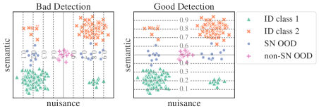
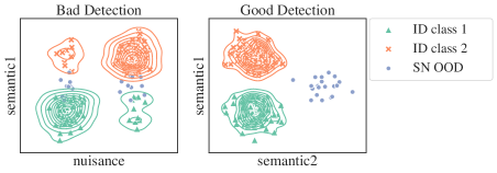
Figure 2: Top: Output-based ood detection will perform poorly on shared-nuisance out-of-distribution inputs when the prediction output relies on nuisance (left) rather than semantics (right), even if non-sn-ood inputs can be detected well in either case. Bottom: Feature-based ood detection is easier when representations focus on semantics (right) rather than both semantics and nuisance (left). Nuisance-aware ood detection encourages the top and bottom right scenarios to improve sn-ood detection.

3 Understanding Shared-Nuisance Out-of-Distribution Detection Failures

To understand sn-ood failures, first note that the success of a classifier for detection depends on the classifier assigning different feature representations or outputs to ood and id inputs. Poor detection of sn-ood inputs relative to non-sn-ood inputs implies that the classifier fails to map sn-ood inputs to outputs or representations sufficiently distinct from those expected of id inputs. Given that both sn-ood and non-sn-ood inputs have unseen semantics, we hypothesize that the difference in performance can be largely explained by how the learned classifier utilizes nuisances. We walk through an output-based and feature-based example below.

To establish notation, let z and y be the nuisance and label which together generate input x. Let $\mathcal{Z}_{tr},\mathcal{Y}_{tr}$ be the values of z and y which appear during training. In semantic ood detection, an input is out-of-distribution if its semantic label was not seen in the training data, i.e. $\textbf{y}\not\in\mathcal{Y}_{tr}$. Then, the difference between shared-nuisance out-of-distribution inputs and non-shared-nuisance out-of-distribution inputs lies in z: sn-ood inputs have nuisances $\textbf{z}\in\mathcal{Z}_{tr}$, while non-sn-ood inputs do not. For instance, for the Waterbirds dataset, a non-bird image over a water background would be a shared-nuisance ood input, while a non-bird image taken indoors would be a non-sn-ood input.

Explaining Poor MSP Performance.

Perfect msp performance requires that all ood inputs have less confident output probabilities than id inputs. Worse detection on sn-ood over non-sn-ood inputs suggests that the former get more peaked confidences in their outputs, making them more similar to id inputs. Since the difference between sn-ood and non-sn-ood inputs is whether $\textbf{z}\in\mathcal{Z}_{tr}$, this worse performance can be attributed to the model’s behavior on $\textbf{z}\in\mathcal{Z}_{tr}$ vs. $\textbf{z}\not\in\mathcal{Z}_{tr}$. Poor sn-ood results suggest that predictive models assign peaked output probabilities to inputs where $\textbf{z}\in\mathcal{Z}_{tr}$ even if $\textbf{y}\not\in\mathcal{Y}_{tr}$. Such a phenomenon is possible if the learned function $f$ is primarily a function of the nuisance, e.g. $f(\textbf{x})\approx g(\textbf{z})$ (Figure 2, top left). Then, sn-ood and id inputs would yield similar outputs, whereas non-sn-ood inputs could yield different outputs and still be detected.

Explaining Poor Mahalanobis Distance Performance.

Mahalanobis distance performs well when ood inputs have representations that are sufficiently different from id ones, enough so to be assigned low density under a model estimating id representations via class-conditional Gaussians. Detection is worse for sn-ood inputs than non-sn-ood ones, suggesting that ood representations are assigned higher density when inputs have nuisance values $\textbf{z}\in\mathcal{Z}_{tr}$. Such a scenario can only occur if nuisance information is present in the representations; otherwise, detection performance of sn-ood and non-sn-ood inputs should be similar, assuming their semantics are similarly different from id semantics.

It is worth noting that, if all the semantic information needed to distinguish id and ood is present in the representations, then a detection method based on perfect density estimation of the id representation distribution would successfully detect ood inputs, regardless of whether the representations additionally contain nuisance information or not. However, in the absence of perfect estimation, representations with more dimensions related to nuisance can be more sensitive to estimation error since they have fewer dimensions dedicated to semantics where id and sn-ood are non-overlapping; for instance, when representations only differ over one dimension, accurate detection requires very accurate modeling of the single relevant dimension, unknown a priori (Figure 2, bottom left). In contrast, representations where id and sn-ood inputs differ over more dimensions are more robust to misestimation over any one dimension (Figure 2, bottom right).

4 Nuisance-Aware OOD Detection

We summarize above observations and explanations below:

1. Observation: Output-based ood detection is worse on sn-ood inputs and degrades with increasing correlation between the nuisance and label in the training distribution. Explanation: The learned predictor adjusts its output based on the nuisance, particularly when there is a strong spurious correlation between nuisance and label in the training data. The result is that sn-ood outputs look like id outputs.

2. Observation: Feature-based ood detection is worse on sn-ood inputs even though its performance is fairly stable across different correlations. Explanation: Regardless of the nuisance-label correlation, the learned representations contain information about the nuisance in addition to semantics, making sn-ood representations look more similar to id ones.

To address both issues, we propose nuisance-aware out-of-distribution detection, utilizing knowledge of nuisances to improve detection. Concretely, to improve output-based detection, we propose substituting a classifier trained via empirical risk minimization with one that is robust to spurious correlations, defined by good classification performance on all distributions that differ from the training distribution in nuisance-label relationship only. Then, to improve feature-based detection, we train a classifier such that its penultimate representation cannot predict the nuisance by itself or conditioned on the label. We motivate and describe our approach below.

Addressing Spurious Correlations via Reweighting

To improve output-based sn-ood detection, we recall that poor output-based sn-ood detection can occur when the learned function $f$ can be approximated by a function of only the nuisance, i.e. $f(\textbf{x})\approx g(\textbf{z})$. Is there a way to avoid learning such functions given only in-distribution data?

First, if a predictor behaves like a function of the nuisance in order to predict the label well on a given data distribution, then it can perform arbitrarily poorly on a new distribution where the relationship between the nuisance and label has changed. Given a data distribution $p_{D}$, let $\mathcal{F}$ be a family of distributions that differ from $p_{D}$ only in the nuisance-label relationship: $\mathcal{F}=\{p_{D^{\prime}}=p_{D}(\textbf{x}\,|\,\textbf{y},\textbf{z})p_{D^{\prime}}(\textbf{z}\,|\,\textbf{y})p_{D}(\textbf{y})\}$, $\text{supp}(p_{D^{\prime}}(\textbf{z}\,|\,\textbf{y}))=\text{supp}(p_{D}(\textbf{z}\,|\,\textbf{y}))$ for all $\textbf{y}\in\text{supp}(p_{D}(\textbf{y}))$. We call the nuisance-label relationship a spurious correlation because it changes across relevant distributions. A predictor that performs well across all distributions in $\mathcal{F}$, i.e. is robust to the spurious correlation between nuisance and label, cannot rely on a function of only nuisance to make its prediction and thus is more likely to succeed at sn-ood detection. In other words, models that are robust to spurious correlations are also likely to be better for output-based sn-ood detection.

Theoretical Motivation.

We propose to improve output-based detection by training models that are robust to spurious correlations. Let ${p_{\scaleto{\perp\!\!\!\perp}{4pt}}}$ be a distribution in $\mathcal{F}$ where the label is independent of the nuisance: $\textbf{z}\perp\!\!\!\perp_{p_{\scaleto{\perp\!\!\!\perp}{4pt}}}\textbf{y}$. Puli et al. (2022a) prove that for all representation functions $r\in\mathcal{R}$ such that $\textbf{z}\perp\!\!\!\perp_{p_{\scaleto{\perp\!\!\!\perp}{4pt}}}\textbf{y}|r(\textbf{x})$, the predictor ${p_{\scaleto{\perp\!\!\!\perp}{4pt}}}(\textbf{y}\,|\,r(\textbf{x}))$ is guaranteed to perform as well as marginal label prediction on any distribution in $\mathcal{F}$, a guarantee that does not always hold outside the set $\mathcal{R}$ where $\textbf{z}\perp\!\!\!\perp_{p_{\scaleto{\perp\!\!\!\perp}{4pt}}}\textbf{y}|r(\textbf{x})$. Moreover, when the identity function is in $\mathcal{R}$, i.e. $\textbf{z}\perp\!\!\!\perp_{p_{\scaleto{\perp\!\!\!\perp}{4pt}}}\textbf{y}|\textbf{x}$, then the predictor ${p_{\scaleto{\perp\!\!\!\perp}{4pt}}}(\textbf{y}\,|\,\textbf{x})$ yields simultaneously optimal performance across all distributions in $\mathcal{F}$ relative to any representation $r\in\mathcal{R}$ and is minimax optimal for a sufficiently diverse $\mathcal{F}$ among all predictors $p_{D}(\textbf{y}\,|\,\textbf{x})$. In other words, ${p_{\scaleto{\perp\!\!\!\perp}{4pt}}}(\textbf{y}\,|\,\textbf{x})$ enjoys substantial performance guarantees when $\textbf{z}\perp\!\!\!\perp_{p_{\scaleto{\perp\!\!\!\perp}{4pt}}}\textbf{y}|\textbf{x}$.

When the input x determines the nuisance z (e.g., looking at an image tells you its background), then $\textbf{z}\perp\!\!\!\perp_{{p_{\scaleto{\perp\!\!\!\perp}{4pt}}}}\textbf{y}\,|\,\textbf{x}$ holds trivially. Consequently, ${p_{\scaleto{\perp\!\!\!\perp}{4pt}}}(\textbf{y}\,|\,\textbf{x})$ has the robustness guarantees summarized above.

Method: Reweighting.

We can estimate ${p_{\scaleto{\perp\!\!\!\perp}{4pt}}}(\textbf{y}\,|\,\textbf{x})$ by reweighting: given $p_{D}(\textbf{x},\textbf{y},\textbf{z})=p_{D}(\textbf{x}\,|\,\textbf{y},\textbf{z})p_{D}(\textbf{y}\,|\,\textbf{z})p_{D}(\textbf{z})$, we can construct ${p_{\scaleto{\perp\!\!\!\perp}{4pt}}}(\textbf{x},\textbf{y},\textbf{z})=p_{D}(\textbf{x}\,|\,\textbf{y},\textbf{z})p_{D}(\textbf{y})p_{D}(\textbf{z})$ as follows (Puli et al. 2022a):

$${p_{\scaleto{\perp\!\!\!\perp}{4pt}}}(\textbf{x},\textbf{y},\textbf{z})=p_{D}(\textbf{x},\textbf{y},\textbf{z})\frac{p_{D}(\textbf{y})}{p_{D}(\textbf{y}\,|\,\textbf{z})}.$$ (1)

We reweight both the training and validation loss using Equation 1 and perform model selection based on the best reweighted validation loss.

Reweighting when Group Labels are Unavailable.

When nuisance values are present as metadata, reweighting based on Equation 1 is straightforward. When we do not have access to exact group labels, following Puli et al. (2022b), we can use functions of the input as nuisance values, e.g. via masking. For instance, for images with centered objects, the outer border of the image can be used as a proxy for background overall. Then, the reweighting mechanism is the same, where a well-calibrated classifier predicting the label from the masked input can approximate $p_{D}(\textbf{y}\,|\,\textbf{z})$.

Addressing Nuisance Features via Independence Constraints

Can we improve feature-based methods on sn-ood inputs, even if they are stable in performance regardless of spurious correlation strength? We hypothesize that removing nuisance information from the learned representations makes id and sn-ood inputs easier to distinguish. First, shared nuisance information is not helpful for distinguishing id and sn-ood inputs by definition, so removing it should not hurt detection performance. Furthermore, when representations contain this information, sn-ood inputs can more easily go undetected, e.g. by looking like id inputs over more of the principal components of variation in the representation. More generally, nuisance information can be additional modeling burden for a downstream feature-based method by introducing additional entropy; for instance, given a discrete representation $r(\textbf{x})$ that is independent of a discrete nuisance, a representation $r^{\prime}(\textbf{x})$ which additionally includes nuisance information (i.e. $p(r^{\prime}(\textbf{x}))=p(r(\textbf{x}),g(\textbf{z}))$) has strictly higher entropy H: $\text{H}(r^{\prime}(\textbf{x}))=\text{H}(r(\textbf{x}))+\text{H}(g(\textbf{z})\,|\,r(\textbf{x}))>\text{H}(r(\textbf{x}))$.

Theoretical Motivation.

To remove nuisance information, we propose enforcing $r(\textbf{x})\perp\!\!\!\perp_{p_{\scaleto{\perp\!\!\!\perp}{4pt}}}\textbf{z}$ and $r(\textbf{x})\perp\!\!\!\perp_{p_{\scaleto{\perp\!\!\!\perp}{4pt}}}\textbf{z}\,|\,\textbf{y}$. The former ensures that the representations cannot predict nuisance on their own, while the latter ensures that within each label class, the representations do not provide information about the nuisance. Without the latter condition, the representations can be a function of nuisance within the id classes such that marginal independence is enforced but sn-ood representations overlap with id ones (see the Appendix A for an example). To avoid this situation and encourage disjoint representations, we enforce marginal and conditional independence, equivalent to joint independence $\textbf{z}\perp\!\!\!\perp_{p_{\scaleto{\perp\!\!\!\perp}{4pt}}}\textbf{y},r(\textbf{x})$.

Method: Joint Independence.

To enforce joint independence, we penalize the estimated mutual information between the nuisance z and the combined representations $r(\textbf{x})$ and label y. When z is high-dimensional, e.g. a masked image, we estimate the mutual information via the density-ratio estimation trick (Sugiyama, Suzuki, and Kanamori 2012), following Puli et al. (2022a). Concretely, we use a binary classifier distinguishing between samples from ${p_{\scaleto{\perp\!\!\!\perp}{4pt}}}(r(\textbf{x}),\textbf{y},\textbf{z})$ and ${p_{\scaleto{\perp\!\!\!\perp}{4pt}}}(r(\textbf{x}),\textbf{y}){p_{\scaleto{\perp\!\!\!\perp}{4pt}}}(\textbf{z})$ to estimate the ratio $\frac{{p_{\scaleto{\perp\!\!\!\perp}{4pt}}}(r(\textbf{x}),\textbf{y},\textbf{z})}{{p_{\scaleto{\perp\!\!\!\perp}{4pt}}}(r(\textbf{x}),\textbf{y}){p_{\scaleto{\perp\!\!\!\perp}{4pt}}}(\textbf{z})}$. When z is low-dimensional, we estimate the mutual information by training a model to predict z from $r(\textbf{x}),\textbf{y}$ under the reweighted distribution ${p_{\scaleto{\perp\!\!\!\perp}{4pt}}}$:

$$\text{I}_{{p_{\scaleto{\perp\!\!\!\perp}{4pt}}}}(\textbf{z};r(\textbf{x}),\textbf{y})$$ (2)

$$=\int{p_{\scaleto{\perp\!\!\!\perp}{4pt}}}(r(\textbf{x}),\textbf{y},\textbf{z})\log\frac{{p_{\scaleto{\perp\!\!\!\perp}{4pt}}}(r(\textbf{x}),\textbf{y},\textbf{z})}{{p_{\scaleto{\perp\!\!\!\perp}{4pt}}}(r(\textbf{x}),\textbf{y}){p_{\scaleto{\perp\!\!\!\perp}{4pt}}}(\textbf{z})}d\textbf{x}d\textbf{y}d\textbf{z}$$ (3)

$$=\mathbb{E}_{{p_{\scaleto{\perp\!\!\!\perp}{4pt}}}}\Big{[}\log\frac{{p_{\scaleto{\perp\!\!\!\perp}{4pt}}}(\textbf{z}\,|\,r(\textbf{x}),\textbf{y})}{{p_{\scaleto{\perp\!\!\!\perp}{4pt}}}(\textbf{z})}\Big{]}.$$ (4)

Other neural network-based mutual information estimators can also be used (Belghazi et al. 2018; Poole et al. 2019). Zero mutual information implies independence; otherwise, there is still dependence, and we add the mutual information as a penalty to the loss when training the main classifier.

Why Naive Independence Doesn’t Work.

Why must we ensure independence of $r(\textbf{x})$ and z under ${p_{\scaleto{\perp\!\!\!\perp}{4pt}}}$ instead of under the original training distribution $p_{D}$? In cases where the nuisance and label are strongly correlated, forcing independence of the penultimate representations and the nuisance will force the representation to ignore information that is predictive of the label, simply because it is also predictive of the nuisance. At one extreme, if the nuisance and label are nearly perfectly correlated under $p_{D}$, then $r(\textbf{x})\perp\!\!\!\perp_{p_{D}}\textbf{z}$ will force $r(\textbf{x})$ to contain almost no information which could predict y. This situation is avoided when label and nuisance are independent.

Summarizing Nuisance-Aware OOD Detection

We propose the following for nuisance-aware ood detection:

1. When performing output-based detection, train a classifier with reweighting: $\mathcal{L}_{{p_{\scaleto{\perp\!\!\!\perp}{4pt}}}}(f(\textbf{x});\textbf{y})$.

2. When performing feature-based detection, train a classifier with reweighting and a joint independence penalty: $\mathcal{L}_{{p_{\scaleto{\perp\!\!\!\perp}{4pt}}}}(f(\textbf{x});\textbf{y})+\lambda\text{I}_{p_{\scaleto{\perp\!\!\!\perp}{4pt}}}(\textbf{z};r(\textbf{x}),\textbf{y})$.

Reweighting is performed based on Equation 1 by estimating $p_{D}(\textbf{y})$ and $p_{D}(\textbf{y}\,|\,\textbf{z})$ from the data. When z is a discrete label, both terms can be estimated by counting the sizes of groups defined by y and z. When z is continuous or high-dimensional, as in a masked image, an additional reweighting model $p_{D}(\textbf{y}\,|\,\textbf{z})$ can be estimated prior to training the main model.

To implement the joint independence penalty, Equation 2 is estimated after every gradient step of the classifier. As described in the above section, one can fit a critic model ${p_{\scaleto{\perp\!\!\!\perp}{4pt}}}(\textbf{z}\,|\,r(\textbf{x}),\textbf{y})$ when z is low-dimensional or employ the density ratio trick when z is high-dimensional. We re-estimate the critic model after each step of the main model training.

5 Why Domain Generalization Methods Fail

Domain generalization algorithms utilize multiple training environments in order to generalize to new test environments. Using knowledge of nuisance to create environments, Ming, Yin, and Li (2022) do not see improved ood detection when training a classifier using domain generalization algorithms implemented in Gulrajani and Lopez-Paz (2021). Here, we explain how, despite taking into account nuisance information, these algorithms can fail to improve output-based sn-ood detection because the resulting models can fail to be robust to spurious correlations.

First, algorithms that rely on enforcing constraints across multiple environments (e.g. Invariant Risk Minimization (irm) (Arjovsky et al. 2019), Risk Extrapolation (rex) (Krueger et al. 2021)) can fail to achieve robustness to spurious correlations if the environments do not have common support, which is typically the case if environments are denoted by nuisance values. In such scenarios, predicting well in one environment does not restrict the model in another environment. The set up in Ming, Yin, and Li (2022) is an example of this scenario, which has also been discussed in Guo et al. (2021) for irm. Instead, to address spurious correlations, these algorithms rely on environments defined by different nuisance-label relationships. However, even then, an irm solution can still fail to generalize to relevant test environments if the training environments available are not sufficiently diverse, numerous, and overlapping (Rosenfeld, Ravikumar, and Risteski 2021). In contrast, nuisance-aware ood detection enables robustness across the family of distributions $\mathcal{F}$ given only one member in the family. Multi-environment objectives can also struggle with difficulty in optimization (Zhang, Lopez-Paz, and Bottou 2022), an additional challenge beyond that of training data availability.

Next, algorithms that enforce invariant representations (e.g. Domain-Adversarial Neural Networks (dann) (Ajakan et al. 2014), Conditional Domain Adversarial Neural Networks (cdann) (Li et al. 2018)) can hurt performance if the constraints imposed are too stringent. For instance, when environments are denoted by nuisance, the constraint posed by dann is equivalent to the naive independence constraint $\textbf{z}\perp\!\!\!\perp r(\textbf{x})$ discussed earlier, which can actively remove semantic information helpful for prediction just because it is correlated with z. cdann enforces the distribution of representations to be invariant across environments conditional on the class label. In Appendix B, we show that a predictor based on the cdann constraint is worse than the nuisance-aware predictor for certain distribution families $\mathcal{F}$. For such $\mathcal{F}$, a cdann predictor is less robust to spurious correlations as measured by performance across the distribution family. Such a predictor will also be worse for sn-ood detection that relies on strong performance over all regions of the in-distribution support in order for id and sn-ood outputs to be as distinct as possible.

Group Distributionally Robust Optimization (gdro) (Sagawa et al. 2020) aims to minimize the worst-case loss over some uncertainty set of distributions, defined by mixtures of pre-defined groups. When the label and nuisance combined define the groups, their mixtures can be seen as distributions with varying spurious correlation strengths. However, other ways of defining groups do not yield the same interpretation; for instance, when the groups are defined by nuisance only, the uncertainty set of distributions is one of varying mixtures of nuisance values while the nuisance-label relationship $p(\textbf{y}\,|\,\textbf{z})$ is held fixed. In other words, such a set up does not address robustness across varying spurious correlations. Even under an appropriate set up for robustness to spurious correlations, gdro may still not reach optimal performance. Concretely, as the loss only depends on the outputs of the worst-performing group, gdro does not favor solutions that continue to optimize performance on other groups if the loss for the worst-performing group is at an local optimum. As intuition, an example where such a situation could occur is one where the best losses possible across groups differs drastically. For an output-based detection method that relies on in-distribution outputs being as large or peaked as possible in order to separate them from ood ones, gdro’s consideration of only worst group performance can hinder detection performance, especially relative to the proposed method which considers all inputs in the reweighting.

6 Related Work

Our work is most closely related to Ming, Yin, and Li (2022) and Puli et al. (2022a). Ming, Yin, and Li (2022) first notice that ood detection is harder on shared-nuisance ood inputs; we expand on their analysis and provide a solution that makes progress on the issue where other approaches (e.g. domain generalization algorithms) do not. Our proposed solution for improving feature-based detection with high-dimensional nuisances, i.e. reweighting and enforcing joint independence, matches the algorithm proposed in Puli et al. (2022a) for ood generalization, though the motivations for each component of the solution are different. Our joint independence algorithm is different for low-dimensional nuisances.

Fort, Ren, and Lakshminarayanan (2021) also demonstrate that classifier choice matters for detection, but they focus on large pretrained transformers, while we consider models that utilize domain knowledge of nuisances. The idea of removing non-discriminative features in the representations of id and ood inputs has also been explored in Kamoi and Kobayashi (2020); Ren et al. (2021), who modify the Mahalanobis distance to consider only a subset of the eigenvectors of the computed covariance matrix. This partial Mahalanobis score focuses on non-sn-ood benchmarks and chooses principal components based on explained variation, whereas we remove shared-nuisance information to address sn-ood failures. More broadly, nuisance-aware ood detection changes the classifier used for detection and can be used alongside other detection methods which employ classifiers.

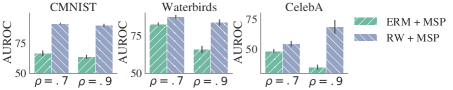
(a) Output-based Detection (msp)

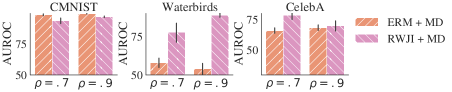
(b) Feature-based Detection (md)

Figure 3: Reweighting (RW) improves output-based sn-ood detection (top), while reweighting and joint independence (RWJI) generally improves feature-based sn-ood detection (bottom). $\rho$ is the strength of the spurious correlation. Results on other methods follow this trend (Appendix Figure 9).

7 Experiments

We consider the following three tasks:

1. CMNIST. $\mathcal{Y}_{tr}=\{0,1\},\mathcal{Z}_{tr}=\{\text{red},\text{green}\}$, $\mathcal{Y}_{\lx@glossaries@gls@link{acronym}{sno}{\leavevmode\textsc{sn-ood}}}=\{2,...,10\}.$

2. Waterbirds. $\mathcal{Y}_{tr}=\{\text{waterbird},\text{landbird}\},\mathcal{Z}_{tr}=\{\text{water},\text{land}\}$, $\mathcal{Y}_{\lx@glossaries@gls@link{acronym}{sno}{\leavevmode\textsc{sn-ood}}}=\{\text{no bird}\}.$

3. CelebA. $\mathcal{Y}_{tr}=\{\text{blond},\text{not blond}\},\mathcal{Z}_{tr}=\{\text{male},\text{female}\}$, $\mathcal{Y}_{\lx@glossaries@gls@link{acronym}{sno}{\leavevmode\textsc{sn-ood}}}=\{\text{bald}\}.$

The open-source datasets from which these tasks are derived all have nuisance metadata available for all examples (e.g. environment label for Waterbirds, attributes for CelebA (Liu et al. 2015)) as well as a way to identify or construct sn-ood examples, enabling us to control both the strength of the spurious correlation in the training set (we consider $\rho\in\{0.7,0.9\}$) while also testing ood detection. We ensure that the dataset sizes are the same across $\rho$. For non-sn-ood datasets, we use blue MNIST digits (Deng 2012) for CMNIST and SVHN (Netzer et al. 2011) for Waterbirds and CelebA. For model architecture, we utilize a 4-layer convolutional network for CMNIST and ResNet-18 pretrained on ImageNet for Waterbirds and CelebA. Unless otherwise noted, we average all results over 5 random seeds, and error bars denote one standard error. We use AUROC as the metric for all detection results following previous literature (Hendrycks and Gimpel 2017). All code, including the hyperparameter configurations for experiments, is available at https://github.com/rajesh-lab/nuisance-aware-ood-detection. See Appendix for more details.

Main Results.

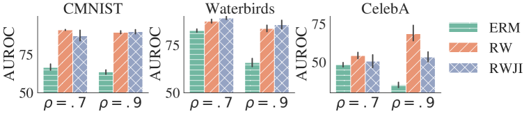
(a) Output-based Detection (msp)

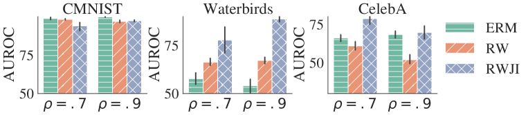
(b) Feature-based Detection (md)

Figure 8: Reweighting (RW) improves output-based sn-ood detection (top), while reweighting and joint independence combined (RWJI) generally improves feature-based sn-ood detection (bottom). This figure reports a larger set of results than Figure 3 in the main paper.

Reweighting substantially improves output-based sn-ood detection (Table 2 in Appendix), providing empirical evidence that increased robustness to spurious correlations (estimated by performance on a new distribution $p_{D^{\prime}}\neq p_{D}$) correlates with improved output-based detection. Reweighting plus joint independence improves feature-based detection with statistically significant results, with the exception of CMNIST, likely due to the task construction where digit is only partially predictive of class (see Appendix D for details), and CelebA at $\rho=0.9$, where joint independence results have high variance. Reversing training strategies and anomaly methods does not the same consistent positive benefit, highlighting the importance selecting the right nuisance-aware strategy for a given detection method (see Figure 8).

While Ming, Yin, and Li (2022) do not see success in combining nuisance information with domain generalization algorithms over their baseline erm solution, Table 1 shows that nuisance-aware ood detection succeeds over nuisance-unaware erm. On non-sn-ood inputs, reweighting yields consistent or better output-based detection performance, and reweighting plus joint independence generally yields comparable or better feature-based detection (Table 3 in Appendix).

	AUROC $\uparrow$
ERM (Ming)	80.98 $\pm$ 2.22
IRM	81.29 $\pm$ 2.62
GDRO	82.94 $\pm$ 2.29
REx	81.25 $\pm$ 2.49
DANN	81.11 $\pm$ 3.10
CDANN	82.13 $\pm$ 1.76
ERM (Ours)	82.14 $\pm$ 1.55
RW	86.86 $\pm$ 1.59

Table 1: On Waterbirds $\rho=0.7$, nuisance-aware ood detection (RW) yields statistically significant improvement over nuisance-unaware detection using erm (energy score, mean $\pm$ standard error over 4 seeds). In contrast, Ming, Yin, and Li (2022) do not see benefit using nuisance information with domain generalization algorithms.

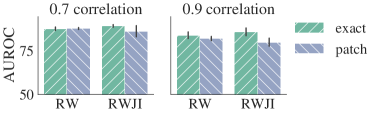
(a) Output-based Detection (msp)

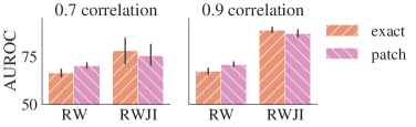
(b) Feature-based Detection (md)

Figure 4: On Waterbirds, using the outer patch as nuisance (patch) yields comparable results to utilizing the exact environment label (exact), which requires external information beyond the image.

Exact vs. User-generated Nuisances.

Unless otherwise specified, experiments use exact nuisances. Even so, Figure 4 shows that that ood detection and balanced id classification results are comparable for Waterbirds whether the nuisance is the exact metadata label or denoted by the outer border of the image. These results illustrate the applicability of nuisance-aware ood detection even when nuisance values are not provided as metadata. Other creative specifications of z are possible, e.g. an image with shuffled pixels if low-level pixel statistics are expected to be a nuisance (Puli et al. 2022b), the representations from a randomly initialized neural network if such representations are expected to be cluster based on nuisance (see Badgeley et al. (2019) for an example).

Other results.

We also consider alternatives to reweighting and joint independence, namely undersampling and marginal independence respectively. We find that undersampling achieves comparable output-based detection but worse feature-based detection and id classification accuracy, and marginal independence yields worse performance than joint independence (Figure 5). We also find that the independence penalty with coefficient $\lambda=1$ yields representations that are less predictive but not completely independent of the nuisance (Table 4 in Appendix) and suspect that removing nuisance information further can improve feature-based sn-ood detection results.

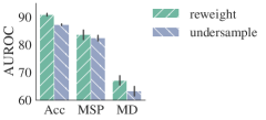
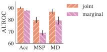
Figure 5: On Waterbirds $\rho=0.9$, undersampling achieves comparable detection results to reweighting but worse balanced accuracy (left). Marginal independence performs worse than joint independence (right).

8 Discussion

Out-of-distribution detection based on predictive models can suffer from poor performance on shared-nuisance ood inputs when the classifier relies on a spurious correlation or its feature representations encode nuisance information. To address these failures, we present nuisance-aware ood detection: to improve output-based detection, we train a classifier via reweighting to estimate ${p_{\scaleto{\perp\!\!\!\perp}{4pt}}}(\textbf{y}\,|\,\textbf{x})$, a distribution that is theoretically guaranteed to be robust to spurious correlations; to improve feature-based detection, we utilize reweighting and a joint independence constraint which encourages representations to be uninformative of the nuisance marginally or conditioned on the semantic class label. Nuisance-aware ood detection yields sn-ood performance benefits for a wide array of existing detection methods, while maintaining performance on non-sn-ood inputs.

However, nuisance-aware ood detection is not without its limitations. First, it requires a priori knowledge of nuisances and a way to specify them for a given task, though there are techniques that handle some missing values (Goldstein et al. 2022). In addition, implementing the joint independence penalty requires training a critic model for each gradient step of the main classifier, an expensive bi-level optimization. Fortunately, once the classifier is trained, prediction (and thus detection) time is no different from that of any other classifier, regardless of how it was trained. We also dox3 not consider feature-based ood detection methods which utilize all layers of a trained network, as such methods typically require validation ood data.

Our work draws a connection between ood generalization and ood detection: classifiers that generalize well across spurious correlations also yield good output-based detection of sn-ood inputs. We believe that future work exploring further connections between ood generalization and detection could be fruitful.

Ethical Statement

Ood detection is an important capability for reliable machine learning, spanning applications from robotics and transportation (e.g. novel object identification) to ecology and public health (e.g. novel species detection). Sn-ood detection focuses on a particularly difficult type of ood input, and improving detection of such inputs can enhance the capabilities of systems across these applications. However, improved ood detection also makes it easier for bad actors to deploy systems which detect anything that strays from the norm they define. Working towards intended applications while keeping in mind potential misuse can help usher in a future of more reliable machine learning systems with positive impact.

9 Acknowledgements

This work was generously funded by NIH/NHLBI Award R01HL148248, NSF Award 1922658 NRT-HDR: FUTURE Foundations, Translation, and Responsibility for Data Science, and NSF CAREER Award 2145542. We thank Aahlad Puli and the anonymous AAAI reviewers for their helpful comments and suggestions.

Appendix A Marginal Independence is Insufficient

Nuisance-aware ood detection proposes joint independence $\textbf{z}\perp\!\!\!\perp_{p_{\scaleto{\perp\!\!\!\perp}{4pt}}}r(\textbf{x}),\textbf{y}$ for feature-based detection rather than only marginal independence $\textbf{z}\perp\!\!\!\perp_{p_{\scaleto{\perp\!\!\!\perp}{4pt}}}r(\textbf{x})$. Below, we provide an example where marginal independence is insufficient to enforce separability between id and sn-ood representations.

Let in-distribution data be defined as the following: $\textbf{y},\textbf{z}\sim\text{Unif}(0,1)$, $\textbf{x}=[\textbf{y},\textbf{z}]$. Assume the representation is limited to be lower dimensional than the input, i.e. 1D representations for 2D input. Let the sn-ood data share the same nuisance values as the id data, i.e. $\textbf{z}\sim\text{Unif}(0,1),$ with out-of-distribution semantics $\textbf{y}\sim\text{Unif}(-1,0)$.

Then, the representation $r_{\text{bad}}(\textbf{x})=\mathbf{1}_{\textbf{z}+\textbf{y}>1}(\textbf{z}+\textbf{y}-1)+\mathbf{1}_{\textbf{z}+\textbf{y}\leq 1}(\textbf{z}+\textbf{y})$ is marginally independent of the nuisance but fails to fully separate id and ood inputs. Concretely, for id inputs, $r_{\text{bad}}(\textbf{x})\sim\text{Unif}(0,1)$, and $r_{\text{bad}}(\textbf{x})\,|\,\textbf{z}\sim\text{Unif}(0,1)$ making it independent from z under the distribution ${p_{\scaleto{\perp\!\!\!\perp}{4pt}}}$: $\textbf{z}\perp\!\!\!\perp_{p_{\scaleto{\perp\!\!\!\perp}{4pt}}}r_{\text{bad}}(\textbf{x})$. For ood inputs, $r_{\text{bad}}(\textbf{x})$ is a triangle distribution between -1 and 1, centered at zero. Because of the support overlap between $r_{\text{bad}}(\textbf{x})$ for id and ood inputs, the representation is unideal for feature-based detection, as perfect detection is impossible (Figure 6a). In contrast, a representation $r_{\text{good}}(\textbf{x})=\textbf{y}$ perfectly separates id and ood inputs (Figure 6b). Intuitively, even though the representations $r_{\text{bad}}(\textbf{x})$ are independent of the nuisance under the in-distribution, the presence of the nuisance in the representation $r_{\text{bad}}(\textbf{x})$ makes id and ood inputs more similar.

We can avoid representations such as $r_{\text{bad}}(\textbf{x})$ by additionally ensuring that $r(\textbf{x})\perp\!\!\!\perp_{p_{\scaleto{\perp\!\!\!\perp}{4pt}}}\textbf{z}\,|\,\textbf{y}$. Then, $r_{\text{bad}}(\textbf{x})=\mathbf{1}_{\textbf{z}+\textbf{y}>1}(\textbf{z}+\textbf{y}-1)+\mathbf{1}_{\textbf{z}+\textbf{y}\leq 1}(\textbf{z}+\textbf{y})$ does not satisfy this constraint, as $p(r_{\text{bad}}(\textbf{x})\,|\,\textbf{y},\textbf{z})\neq p(r_{\text{bad}}(\textbf{x})\,|\,\textbf{z})$; the left-hand side is a Dirac distribution as $r_{\text{bad}}(\textbf{x})$ is fully determined by y and z, whereas the right-hand side is a Uniform distribution.

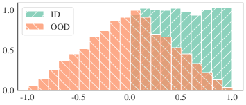
(a) $r_{\text{bad}}(\textbf{x})$

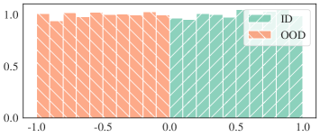
(b) $r(\textbf{x})=\textbf{y}$

Figure 6: The representation $r$ can be independent of z yet still not separate id and ood inputs (top), as the representation can still depend on z conditional on the label. Additionally enforcing independence conditional on y addresses such scenarios and yields to more desirable representations (bottom).

The example for $r_{\text{bad}}$ is inspired by Puli and Ranganath (2020), who also note that the construction can be generalized to other continuous distributions using the probability integral transform or universality of the uniform. The function that defines $r_{\text{bad}}$ is also used to establish challenges in conditional independence testing (Sudarshan et al. 2022).

Appendix B CDANN vs. Nuisance-Aware Predictor

Here we offer an explanation for why the cdann predictor performs worse than the nuisance-aware predictor on sn-ood detection by comparing both predictors with respect to their robustness to spurious correlations. While cdann was not developed specifically with generalization across spurious correlations in mind, first we translate the cdann objective into the framework proposed in Puli et al. (2022a). Then, we show that the cdann constraint results in a predictor that performs worse over certain distribution families $\mathcal{F}$ than the nuisance-aware predictor.

First, we show that the cdann predictor, i.e. $p_{D}(\textbf{y}\,|\,r(\textbf{x}))$ where $\textbf{z}\perp\!\!\!\perp r(\textbf{x})\,|\,\textbf{y}$, is equivalent to the predictor ${p_{\scaleto{\perp\!\!\!\perp}{4pt}}}(\textbf{y}\,|\,r(\textbf{x}))$ where $\textbf{z}\perp\!\!\!\perp_{p_{\scaleto{\perp\!\!\!\perp}{4pt}}}r(\textbf{x}),\textbf{y}$. Recall that all distributions in $\mathcal{F}$ share the same $p(r(\textbf{x})\,|\,\textbf{y},\textbf{z})$ and $p(\textbf{y})$, and that ${p_{\scaleto{\perp\!\!\!\perp}{4pt}}}(\textbf{z}\,|\,\textbf{y})=p_{D}(\textbf{z})$.

$$p_{D}(\textbf{y}\,|\,r(\textbf{x})) =\frac{p_{D}(\textbf{y},r(\textbf{x}))}{p_{D}(r(\textbf{x}))}$$

$$=\frac{\int p_{D}(\textbf{y},r(\textbf{x}),\textbf{z})d\textbf{z}}{\int\int p_{D}(\textbf{y},r(\textbf{x}),\textbf{z})d\textbf{z}d\textbf{y}}$$

$$=\frac{\int p_{D}(r(\textbf{x})\,|\,\textbf{y},\textbf{z})p_{D}(\textbf{z}\,|\,\textbf{y})p_{D}(\textbf{y})d\textbf{z}}{\int\int p_{D}(r(\textbf{x})\,|\,\textbf{y},\textbf{z})p_{D}(\textbf{z}\,|\,\textbf{y})p_{D}(\textbf{y})d\textbf{z}d\textbf{y}}$$

$$=\frac{\int p_{D}(r(\textbf{x})\,|\,\textbf{y})p_{D}(\textbf{z}\,|\,\textbf{y})p_{D}(\textbf{y})d\textbf{z}}{\int\int p_{D}(r(\textbf{x})\,|\,\textbf{y})p_{D}(\textbf{z}\,|\,\textbf{y})p_{D}(\textbf{y})d\textbf{z}d\textbf{y}}$$

$$=\frac{p_{D}(r(\textbf{x})\,|\,\textbf{y})p_{D}(\textbf{y})\int p_{D}(\textbf{z}\,|\,\textbf{y})d\textbf{z}}{\int\big{(}\int p_{D}(\textbf{z}\,|\,\textbf{y})d\textbf{z}\big{)}p_{D}(r(\textbf{x})\,|\,\textbf{y})p_{D}(\textbf{y})d\textbf{y}}$$

$$=\frac{p_{D}(r(\textbf{x})\,|\,\textbf{y})p_{D}(\textbf{y})}{\int p_{D}(r(\textbf{x})\,|\,\textbf{y})p_{D}(\textbf{y})d\textbf{y}}$$

$$=\frac{p_{D}(r(\textbf{x})\,|\,\textbf{y})p_{D}(\textbf{y})\int{p_{\scaleto{\perp\!\!\!\perp}{4pt}}}(\textbf{z}\,|\,\textbf{y})d\textbf{z}}{\int\big{(}\int{p_{\scaleto{\perp\!\!\!\perp}{4pt}}}(\textbf{z}\,|\,\textbf{y})d\textbf{z}\big{)}p_{D}(r(\textbf{x})\,|\,\textbf{y})p_{D}(\textbf{y})d\textbf{y}}$$

$$=\frac{\int p_{D}(r(\textbf{x})\,|\,\textbf{y}){p_{\scaleto{\perp\!\!\!\perp}{4pt}}}(\textbf{z}\,|\,\textbf{y})p_{D}(\textbf{y})d\textbf{z}}{\int\int p_{D}(r(\textbf{x})\,|\,\textbf{y}){p_{\scaleto{\perp\!\!\!\perp}{4pt}}}(\textbf{z}\,|\,\textbf{y})p_{D}(\textbf{y})d\textbf{z}d\textbf{y}}$$

$$=\frac{\int p_{D}(r(\textbf{x})\,|\,\textbf{y},\textbf{z}){p_{\scaleto{\perp\!\!\!\perp}{4pt}}}(\textbf{z}\,|\,\textbf{y})p_{D}(\textbf{y})d\textbf{z}}{\int\int p_{D}(r(\textbf{x})\,|\,\textbf{y},\textbf{z}){p_{\scaleto{\perp\!\!\!\perp}{4pt}}}(\textbf{z}\,|\,\textbf{y})p_{D}(\textbf{y})d\textbf{z}d\textbf{y}}$$

$$=\frac{{p_{\scaleto{\perp\!\!\!\perp}{4pt}}}(\textbf{y},r(\textbf{x}))}{{p_{\scaleto{\perp\!\!\!\perp}{4pt}}}(r(\textbf{x}))}$$

$$={p_{\scaleto{\perp\!\!\!\perp}{4pt}}}(\textbf{y}\,|\,r(\textbf{x})).$$

$$\textbf{z}\perp\!\!\!\perp r(\textbf{x})\,|\,\textbf{y} \implies\textbf{z}\perp\!\!\!\perp_{p_{\scaleto{\perp\!\!\!\perp}{4pt}}}r(\textbf{x})\,|\,\textbf{y}\implies\textbf{z}\perp\!\!\!\perp_{p_{\scaleto{\perp\!\!\!\perp}{4pt}}}r(\textbf{x}),\textbf{y}.$$ (5)

The first implication in Equation 5 follows from the fact that all distributions in $\mathcal{F}$ share the same $p(r(\textbf{x})\,|\,\textbf{y},\textbf{z})$, which in this case is equivalent to $p(r(\textbf{x})\,|\,\textbf{y})$.

Puli et al. (2022a) prove that there exist distribution families $\mathcal{F}$ where predictors using representations under the constraint $\textbf{z}\perp\!\!\!\perp_{p_{\scaleto{\perp\!\!\!\perp}{4pt}}}r(\textbf{x}),\textbf{y}$ are suboptimal relative to predictors which enforce representations to satisfy $\textbf{z}\perp\!\!\!\perp_{p_{\scaleto{\perp\!\!\!\perp}{4pt}}}\textbf{y}\,|\,r(\textbf{x})$. Concretely, for certain distribution families $\mathcal{F}$, the prediction performance of the former (i.e. the cdann predictor) is no better than that of the latter (i.e. the nuisance-aware predictor) on any distribution in $\mathcal{F}$ and strictly worse on at least one. The result implies that the cdann predictor is less robust to spurious correlations (based on performance over the distributions $p_{D}\in\mathcal{F}$), meaning such a predictor is worse for sn-ood detection which relies on strong classification performance over all $p_{D}\in\mathcal{F}$ in order to ensure that id outputs are distinct from ood ones.

Appendix C Experimental Set Up

Datasets

We generate the following three benchmark tasks from existing open-source datasets. In all datasets, the training and validation set have the same correlation between nuisance and label (specified by $\rho$), and the test set is balanced.

CMNIST.

Following Arjovsky et al. (2019), we generate different datasets of red and green MNIST digits; digit is correlated with label 75% of the time, and color is correlated with label differently for each dataset denoted by $\rho$ (i.e. 0.7, 0.9). Unlike Arjovsky et al. (2019), we use only the digits 0 and 1 as in-distribution inputs, leaving the other digits as out-of-distribution.

Waterbirds.

Following Ming, Yin, and Li (2022), we use the Waterbirds dataset generation code from Sagawa et al. (2020), generating a different dataset for each correlation strength. We give the validation set the same correlation as the training set, rather than balancing it as done in Sagawa et al. (2020). We use a subset of the land and water images from PlacesBG dataset (Zhou et al. 2018) for sn-ood inputs, also following (Ming, Yin, and Li 2022).

CelebA.

Following Sagawa et al. (2020), we use the CelebA dataset of celebrity attributes (Liu et al. 2015) and generate two datasets with different correlations of the blond hair and gender attributes. We set the train, validation, and test sets to 5548, 728, and 720 respectively for each dataset generated; these numbers are the maximum dataset sizes possible for each of the predefined splits while enabling all correlation strengths without duplicates. We note that our choice of label (i.e. blond hair) differs from Ming, Yin, and Li (2022) who use grey hair but matches that of Sagawa et al. (2020). Following Ming, Yin, and Li (2022), we use no hair images as sn-ood inputs.

To our knowledge, we are not aware of offensive content in the datasets used for this work, though the CelebA dataset does contain less appropriate attributes (i.e. attractive or not) which we do not make use of in our experiments. We also recognize the CelebA dataset is biased in the individuals represented.

Experiment Details

Models.

For Waterbirds and CelebA, we use a ResNet-18 (He et al. 2016) pretrained on ImageNet. For CMNIST we use a 4-layer neural network of 2D convolution-batch norm-relu blocks with 32 7x7 filters each, followed by a final linear layer. All models output two logits to perform binary classification rather than one. This choice makes it possible for output-based methods such as max logit, energy score, and maximum softmax probability to yield different rankings across inputs. When $p_{D}(\textbf{y}\,|\,\textbf{z})$ needs to be estimated given a high-dimensional nuisance z, we use the same architecture for the reweighting model as well. Otherwise, we estimate the weights for reweighting based on the group counts in the training data. For Waterbirds, where there is also label imbalance, our weights additionally balance the label marginals in addition to breaking the correlation between label and nuisance.

To estimate mutual information when encouraging joint independence, we also have an additional critic model. When z is low dimensional, the model ${p_{\scaleto{\perp\!\!\!\perp}{4pt}}}(\textbf{z}\,|\,\textbf{y},r(\textbf{x}))$ is a multilayer perceptron with 2 hidden layers, 256 and 128 hidden units respectively, and relu non-linearities. When z is high-dimensional, the model classifying between ${p_{\scaleto{\perp\!\!\!\perp}{4pt}}}(r(\textbf{x}),\textbf{y},\textbf{z})$ and ${p_{\scaleto{\perp\!\!\!\perp}{4pt}}}(r(\textbf{x}),\textbf{y}){p_{\scaleto{\perp\!\!\!\perp}{4pt}}}(\textbf{z})$ first maps y and z to representations of the same dimension as $r(\textbf{x})$, using a single fully connected layer with relu non-linearity for y and a network for z whose architecture matches that of the main classifier. Then, the representations are concatenated on the channel dimension and pass through two 1D convolution layers (single 3x3 filter each) with relu non-linearities before a final linear layer to the output.

Training.

We train CMNIST and Waterbirds for 30 epochs and CelebA for 100 epochs. We train a CMNIST and Waterbirds reweighting models for 20 epochs and CelebA reweighting models for 50. We checkpoint models at the end of every epoch and select the model with the best validation loss. We use reweighted validation loss for main models on nuisance-aware runs. We train the critic models for 2 epochs between every gradient step. All training runs utilize the Adam optimizer with a learning rate of 1e-5, weight decay of 5e-3, and momentum of 0.9. Following Ming, Yin, and Li (2022), we adjust the learning rate using a cosine annealing schedule for the main model and reweighting model. We utilize RTX8000 and V100 GPUs, with training runs lasting from several minutes to several days depending on the experiment.

Appendix D Additional Results & Analysis

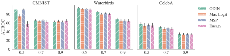
Figure 7: Output-based methods struggle to detect sn-ood inputs and get worse as the strength of the spurious correlation increases (x-axis is the nuisance-label correlation $\rho$). All methods perform similarly to MSP, pictured in the results of the main paper (Figure 1).

Exception to the trend that joint independence generally improves feature-based detection.

In the bottom row of Figure 3, we show that reweighting plus joint independence generally improves feature-based detection. One exception, CMNIST, is likely due to the task construction where digit is only partially predictive of label. Since both label classes contain instances of both digits, per-class representations based on digit information alone will be bimodal (one mode per digit). Then, for Mahalanobis distance-based detection, the estimated class-conditional Gaussians will place the highest density in between the clusters rather than where the data samples reside. Including nuisance information can improve detection by increasing the density assigned to in-distribution samples on average. Concretely, by allowing for more samples within a given class to be correctly classified, nuisance information enables the largest mode within a given class to be larger than it would be if nuisance were not present in the representations. As a result, class-conditional Gaussians fit to the representations will be closer to the largest mode and assign those samples higher density. Then, joint independence can hurt detection by removing nuisance information that would otherwise improve how well the representations adhere to the assumptions of Mahalanobis distance. When there are semantic features that can perfectly predict the label, on the other hand, we expect that joint independence will not hurt and will generally improve detection performance, as seen on the other datasets.

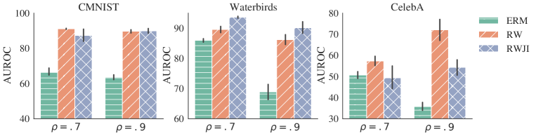
(a) ODIN

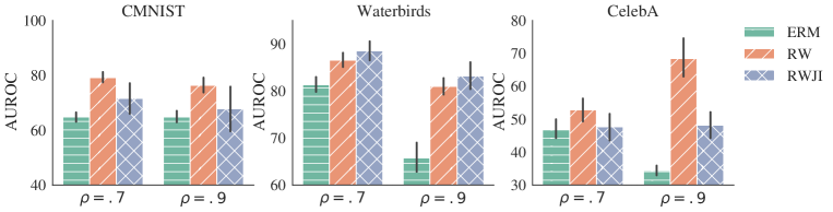
(b) Max Logit

(c) Energy

Figure 9: Reweighting improves performance across tasks and different output-based methods. Results follow a similar pattern to those of msp, shown in Figure 3 in the main paper. One exception is energy-based ood detection on CMNIST; as results improve for other methods on the same task and other tasks using the same method, this exception implies that for CMNIST in particular, the largest logits become more separable between id and ood but a sum aggregation of the logits does not.

		CMNIST	Waterbirds	CelebA
0.7	ERM	69.66 $\pm$ 2.13	93.12 $\pm$ 0.45	89.14 $\pm$ 0.63
	RW	73.93 $\pm$ 0.05	92.94 $\pm$ 0.40	90.16 $\pm$ 0.48
	RWJI	73.60 $\pm$ 0.47	88.82 $\pm$ 0.79	90.12 $\pm$ 0.64
0.9	ERM	48.89 $\pm$ 0.00	89.36 $\pm$ 0.84	84.65 $\pm$ 0.71
	RW	75.91 $\pm$ 0.35	90.92 $\pm$ 0.85	88.95 $\pm$ 0.74
	RWJI	76.12 $\pm$ 0.10	89.97 $\pm$ 1.47	88.59 $\pm$ 0.61

Table 2: Models trained with reweighting have better balanced test accuracy performance than models trained with erm. The fact that models trained with reweighting also have better output-based detection performance (see Figure 3) suggests that improved robustness of spurious correlations is correlated with improved output-based detection. Results are mean $\pm$ 2 standard errors.

			Maximum Softmax Probability	Mahalanobis Distance
CMNIST	0.7	ERM	73.5541 $\pm$ 2.1341	99.4762 $\pm$ 0.2364
		RW	96.3765 $\pm$ 1.0356	98.5469 $\pm$ 0.5968
		RWJI	94.2829 $\pm$ 2.3302	65.0447 $\pm$ 21.7247
	0.9	ERM	85.0077 $\pm$ 6.1215	99.8607 $\pm$ 0.0547
		RW	93.1736 $\pm$ 1.3446	99.0073 $\pm$ 0.3461
		RWJI	94.6013 $\pm$ 2.2847	92.3193 $\pm$ 3.7097
Waterbird	0.7	ERM	96.9957 $\pm$ 0.4732	98.4097 $\pm$ 0.2125
		RW	97.0512 $\pm$ 0.5570	97.2273 $\pm$ 0.3499
		RWJI	90.5908 $\pm$ 1.4941	100.0000 $\pm$ 0.0000
	0.9	ERM	91.5222 $\pm$ 0.9527	99.0138 $\pm$ 0.1265
		RW	96.3132 $\pm$ 0.4235	98.4988 $\pm$ 0.1844
		RWJI	69.7826 $\pm$ 5.3348	100.0000 $\pm$ 0.0000
CelebA	0.7	ERM	94.4956 $\pm$ 0.7544	99.6800 $\pm$ 0.0696
		RW	94.3586 $\pm$ 0.7463	99.6844 $\pm$ 0.0925
		RWJI	86.8020 $\pm$ 3.5929	100.0000 $\pm$ 0.0000
	0.9	ERM	94.1410 $\pm$ 1.1558	99.8080 $\pm$ 0.0651
		RW	93.2244 $\pm$ 1.8937	99.7184 $\pm$ 0.0752
		RWJI	86.5786 $\pm$ 4.1056	100.0000 $\pm$ 0.0000

Table 3: On a non-sn-ood dataset (blue MNIST 2-9 for CMNIST, SVHN for Waterbirds or CelebA), reweighting yields consistent or better output- and feature-based detection performance, and adding joint independence generally yields consistent or better feature-based detection. The exception to the latter is CMNIST, likely due to the synthetic set up where semantics (digit) are only partially predictive of the id labels; in this set up, the per-class representations based on semantics alone are likely less well-clustered (i.e. some zero digits are in the zero class and others are in the one class), breaking the assumption that semantics-only representations are sufficient. Thus, joint independence may be hurting detection performance by removing helpful color information, and high variance between seeds may be due to optimization. Joint independence also hurts output-based detection, likely due to optimization difficulties which lead to a suboptimal learned predictor function.

		CMNIST	Waterbirds	CelebA
0.7	ERM	0.9986 $\pm$ 0.0008	0.9210 $\pm$ 0.0035	0.8515 $\pm$ 0.0169
	RW	0.9991 $\pm$ 0.0008	0.9231 $\pm$ 0.0025	0.8459 $\pm$ 0.0157
	RWJI	0.9122 $\pm$ 0.0323	0.7398 $\pm$ 0.0138	0.6723 $\pm$ 0.0123
0.9	ERM	0.9995 $\pm$ 0.0004	0.9349 $\pm$ 0.0018	0.8753 $\pm$ 0.0090
	RW	0.9986 $\pm$ 0.0009	0.9265 $\pm$ 0.0014	0.8519 $\pm$ 0.0130
	RWJI	0.9588 $\pm$ 0.0169	0.7449 $\pm$ 0.0167	0.7205 $\pm$ 0.0127

Table 4: Joint independence makes representations less predictive of but not completely independent of the nuisance, i.e. representations from joint independence are worse at predicting nuisance than representations from erm or reweighting but better than random chance. Results are AUROC for the prediction of exact nuisance labels performed with 100 gradient-boosted trees optimizing log loss.

Different Waterbirds Generation Seeds Yield Datasets of Varying Difficulties

Waterbirds is a semi-synthetic dataset generated by placing birds in front of water and land backgrounds. Following Ming, Yin, and Li (2022), we use the generation script provided by Sagawa et al. (2020) to generate a separate dataset for each spurious correlation strength. However, after collecting the main results in the paper, we noticed that the failure mode numbers in Figure 1 were quite different from those of Ming, Yin, and Li (2022); subsequently, we tested various seeds to see whether we could reproduce the failure mode numbers. In doing so, we found that the stochasticity in the generation process resulted in datasets of varying difficulty; namely, Figure 10 below shows drastically different results for the baseline depending on the seed used to generate the data (i.e. different heights for green bars with horizontal stripes). We subsequently tested three additional seeds and found that while the absolute numbers vary significantly across seeds, the trend reported in the main paper remains consistent: reweighting improves output-based detection, and reweighting plus joint independence generally improves feature-based detection.

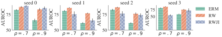
(a) Output-based Detection (msp)

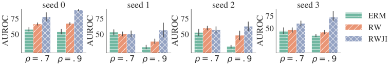
(b) Feature-based Detection (md)

Figure 10: While different generation seeds yield different absolute results, the trend reported in the paper is robust to this stochasticity: reweighting (RW) improves output-based sn-ood detection (top), while reweighting and joint independence combined (RWJI) generally improves feature-based sn-ood detection (bottom).

References

- Ajakan et al. (2014) Ajakan, H.; Germain, P.; Larochelle, H.; Laviolette, F.; and Marchand, M. 2014. Domain-Adversarial Neural Networks. arXiv preprint arXiv:1412.4446.
- Arjovsky et al. (2019) Arjovsky, M.; Bottou, L.; Gulrajani, I.; and Lopez-Paz, D. 2019. Invariant Risk Minimization. ArXiv, abs/1907.02893.
- Badgeley et al. (2019) Badgeley, M. A.; Zech, J. R.; Oakden-Rayner, L.; Glicksberg, B. S.; Liu, M.; Gale, W.; McConnell, M. V.; Percha, B. L.; Snyder, T. M.; and Dudley, J. T. 2019. Deep learning predicts hip fracture using confounding patient and healthcare variables. NPJ Digital Medicine, 2.
- Belghazi et al. (2018) Belghazi, M. I.; Baratin, A.; Rajeswar, S.; Ozair, S.; Bengio, Y.; Hjelm, R. D.; and Courville, A. C. 2018. Mutual Information Neural Estimation. In ICML.
- Bishop (1994) Bishop, C. M. 1994. Novelty detection and neural network validation. IEE Proceedings-Vision, Image and Signal processing, 141(4): 217–222.
- Deng (2012) Deng, L. 2012. The mnist database of handwritten digit images for machine learning research. IEEE Signal Processing Magazine, 29(6): 141–142.