Hyperspectral Image Compression Using Implicit Neural Representation

Abstract

Hyperspectral images, which record the electromagnetic spectrum for a pixel in the image of a scene, often store hundreds of channels per pixel and contain an order of magnitude more information than a typical similarly-sized color image. Consequently, concomitant with the decreasing cost of capturing these images, there is a need to develop efficient techniques for storing, transmitting, and analyzing hyperspectral images. This paper develops a method for hyperspectral image compression using implicit neural representations where a multilayer perceptron network $\Phi_{\theta}$ with sinusoidal activation functions “learns” to map pixel locations to pixel intensities for a given hyperspectral image $I$. $\Phi_{\theta}$ thus acts as a compressed encoding of this image. The original image is reconstructed by evaluating $\Phi_{\theta}$ at each pixel location. We have evaluated our method on four benchmarks—Indian Pines, Cuprite, Pavia University, and Jasper Ridge—and we show the proposed method achieves better compression than JPEG, JPEG2000, and PCA-DCT at low bitrates.

1 Introduction

Hyperspectral images capture electromagnetic spectrum for a pixel in the image of a scene  [31, 21]. These images offer many possibilities for object detection, material identification, and scene analysis. The costs associated with capturing high-resolution temporal, spatial, and spectral data continue to decrease, and it is no surprise that hyperspectral images have found widespread use in areas such as, remote sensing, biotechnology, crop analysis, environmental monitoring, food production, medical diagnosis, pharmaceutical industry, mining, and oil & gas exploration, etc. [20, 24, 2, 19, 33, 9, 3, 30, 48, 41, 17, 25, 18, 12]. Unlike color images that record red, green, and blue channels per pixel, hyperspectral images record 100s of channels per pixel, representing pixels’ spectra. This suggests that hyperspectral images require two orders of magnitude more space than what is needed to store similarly-sized color images. Consequently, there is a need to develop efficient schemes for capturing, storing, transmitting, and analyzing hyperspectral images. This work studies hyperspectral image compression which plays an important role in the storage and transmission of these images.

Recently, there has been a surge in interest in learning-based compression schemes. For example, autoencoders [1] and rate-distortion autoencoders [4, 5] have been used to learn compact representations of the input signals. Here network weights together with the signal signature—latent representation in the case of autoencoders—serve as the compressed representation of the input signal. Other concurrent works are exploring the use of Implicit Neural Representations (INRs) for signal compression. INRs are well-suited to represent data that lives on an underlying grid, and these offer a new paradigm for signal representation. The goal here is to learn a mapping between a location, say an $(x,y)$ pixel location for a 2D-image $I$, and the signal value at that location $I[x,y]$. This mapping is subsequently used to recreate the original signal. It is as simple as evaluating the INR at various locations. In the case of INRs, network weights serve as the learned representation of the input signal.

We investigate the use of INRs for hyperspectral image compression and show that it is possible to achieve high rates of compression while maintaining acceptable reconstruction quality. We evaluate the proposed approach on four benchmarks—Jasper Ridge, Indian Pines, Pavia University, and Cuprite—against three approaches—JPEG [23, 44], PCA-DCT [38], and JPEG2000 [14] —that others have used to compress hyperspectral data. The results confirm that our method achieves a better Peak Signal-to-Noise ratio (PSNR) at low compression rates than those obtained by other methods.

The rest of the paper is organized as follows. We discuss related works in the next section. Section Method describes the Image compression using implicit neural representation method and the pipeline of our proposed method. Next, we present the experimental setup and discuss the results. Section conclusions conclude a paper with a summary and possible directions for future work.

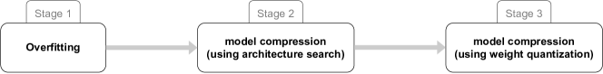
Figure 1: Overview of INR-based compression pipeline comprising overfitting, model compression using architecture search, and model compression using weight quantization.

2 Related work

Hyperspectral images exhibit both spatial and spectral redundancies that can be exploited to achieve compression. Lossless compression schemes—e.g., those that use quantization or rely upon entropy-coding or statistics-based schemes—where it is possible to recover the original signal precisely often do not yield large savings [35, 40]. Lossy compression schemes, on the other hand, promise large savings while maintaining acceptable reconstruction quality. Inter-band compression techniques aim to eliminate spectral redundancy [10], while intra-band compression techniques aim to exploit spatial correlations. Intra-band compression techniques often follow the ideas developed for typical color image compression. [56] exploit the fact that groups of pixels that are around the same location in two adjacent bands are strongly correlated and proposes schemes that perform both inter-band and intra-band compression. Principal Component Analysis (PCA) based techniques are frequently used for hyperspectral image compression. PCA offers strong spectral decorrelation and is used to reduce the number of channels in a hyperspectral image. The remaining channels are subsequently compressed using Joint Picture Expert Group (JPEG) or JPEG2000 standard [7, 15, 53, 43]. Along similar lines, tensor decomposition methods have also been applied to the problem of hyperspectral image compression [55]. Tensor decomposition achieves dimensionality reduction while maintaining the spatial structure. Transform coding schemes that achieve image compression by reducing spatial correlation have also been used to compress hyperspectral data. Discrete Cosine Transform (DCT) has been used to perform intra-band compression; however, it ignores iner-band (or spectral) redundancy. 3D-DCT that divides a 3-dimensional hyperspectral image into $8\times 8\times 8$ datacubes is proposed to achieve both inter-band and intra-band compression [45]. Similarly to JPEG, which uses $8\times 8$ blocks, 3D-DCT exhibits blocking effects in reconstructed hyperspectral images. The blocking effects can be removed to some extent by using wavelet transform instead [46, 22]. Video coding methods coupled with inter-band spectral prediction modeling have also been proposed to compress hyperspectral images.

3 Method

3.1 Background

In the 3D vision field, interest in using neural networks to represent data has recently increased [39, 42, 11], after the original proposal made by [50]. High-resolution signals can be compactly encoded via implicit representations, as suggested by studies [36, 49, 51].

Commonly, learned image compression techniques use hierarchical variational autoencoders [6, 32, 37], where the latent variables are discretized for entropy coding purpose. Paper [16] proposes a different approach for RGB image compression. Their method stores the weights of a neural network overfitted to the image.  Similar to previous research on latent variable models [27, 28, 29, 34], numerous studies [8, 26, 54] make an effort to close the amortization gap [13] by combining the usage of amortized inference networks with iterative gradient-based optimization procedures. Using inference time per instance optimization, [54] also identifies and makes an effort to bridge the discretization gap caused by quantizing the latent variables. The concept of per-instance model optimization is expanded upon in research [52], which fine-tunes the decoder for each instance and transmits updates to the quantized decoder’s parameters together with the latent code to provide better rate-distortion performance.

Figure 2: Compressed neuronal representations that are implicit. A neural network that maps pixel positions (x, y) to channel values are used to overfit an image. The weights of this neural network are then transmitted after being quantized to a smaller bit-width.

3.2 Image Compression using INRs

INRs represent data as a continuous function from coordinates to values, storing coordinate-based data like photos, videos, and 3D forms. For instance, hyperspectral image maps to a channel vector in a channel space based on the horizontal and vertical coordinates $(p_{x},p_{y})$:

$$I:(p_{x},p_{y})\rightarrow(ch_{0},ch_{1},...,ch_{n}),$$ (1)

In which ch refers to channels, and n equals the number of channels for each image. A neural network $f_{\Theta}$, often a Multi-Layer Perceptron (MLP) with parameters $\Theta$, can be used to approximate this mapping such that $I(p_{x},p_{y})\approx f_{\Theta}(p_{x},p_{y})$. INRs can be evaluated on any coordinates inside the normalized range [1, 1] since they are continuous functions.

INRs implicitly store all data in the network weights. The coordinate, which is used as the input to the INR, contains no information. The INR is trained through the encoding procedure. Decoding is the same as adding a set of weights to the network and assessing the results on a coordinate grid. This can be summed up as:

$$\arg\min_{\theta}L(x,f_{\theta}(p))=\theta^{*}\xrightarrow[transmit\theta^{*}]{}\widehat{X}=f_{\theta^{*}}(p).$$ (2)

In order to recreate a distorted replica of the original image X, we just need to store $\Theta^{\star}$. With our strategy, we are able to simultaneously accomplish compact storage and effective repair.

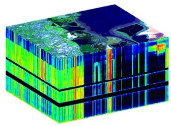
Figure 3: The JPL’s AVIRIS hyperspectral data cube provided on a NASA ER-2 plane over Moffett Field

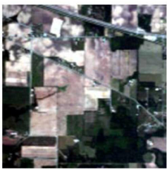
(a)

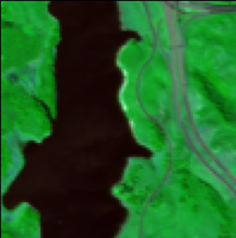
(b)

(c)

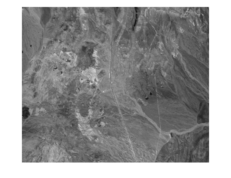
(d)

Figure 4: From left to right, datasets: Indian Pines, Jasper Ridge, Pavia University, and Cuprite.

3.3 Compression Pipeline for INRs

The pipeline for our INR-based compression is described in this section. Figure 1 represent the entire pipeline and figure 2 shows a higher-level overview.
Stage 1: Overfitting. We train an MLP to map pixel locations to pixel values in this work. In fact, at test time, we overfit the INR f to a data sample. This step is similar to calling the encoder in other learned techniques. To underline that the INR is trained only to represent one image, we refer to this stage as overfitting.

We save the weights of a neural network overfitted to the image rather than the pixel values for each pixel of a hyperspectral image. A general illustration of this work is proposed in Figure 2. To encode an image, we apply an MLP, which maps pixel locations to pixel values. We test the MLP at each pixel position to decode the image. While the extremely frequent data included in some hyperspectral images makes overfitting such multi-layer perceptrons, also known as implicit neural representations, challenging [47, 51], recent studies have demonstrated that this can be minimized by employing sinusoidal encodings and activations [51, 36, 49]. As a result, in this study, we use MLPs with sine activations, often known as SIRENs [49].
As a result, we first overfit an MLP to the hyperspectral image, then quantize and transmit its weights. To reconstruct the hyperspectral image, the transmitted MLP is then evaluated at all pixel positions. Let I represent the hyperspectral image we want to encode, and $I[x,y]$ gives the pixel values at that specific pixel position for the encoding part $(x,y)$. In the hyperspectral image, we build a function $f_{\Theta}$ with parameters $\Theta$ mapping pixel positions to pixel band values. The hyperspectral image can then be encoded by overfitting $f_{\Theta}$ to it under some distortion control. Given an image x and a coordinate grid p, we minimize the objective:

$$\arg\min_{\theta}L_{MSE}(x,f_{\theta}(p)).$$ (3)

The parameterization of $f_{\Theta}$ must be carefully chosen. Even when utilizing quite a few parameters, parameterizing $f_{\Theta}$ using an MLP with normal activation functions leads to underfitting [51, 49]. We choose the sine activation function for this work, according to [49].
Stage 2: Model Compression using Architecture Search. We run a hyperparameter tunning over the number of layers and layer size of the MLP and also quantize the weights from 32-bit to 16-bit precision to decrease the model size. As a result, we explore architecture search and weight quantization strategies to decrease model size.
Stage 3: Model Compression using Weight Quantization. Because the MLP parameters are stored as a compressed representation of the image, limiting the number of weights improves compression. The purpose is to fit $f_{\Theta}$ to I with the fewest parameters possible. The hyperspectral images are then compressed using model compression.
Decoding part is to just evaluate the function $f_{\Theta}$ at each pixel position to rebuild the image given the stored quantized weights. This decoding method provides several advantages, such as increased flexibility: we may decode the image in stages, for instance, by decoding portions of it or a low-resolution image initially, just by assessing $f_{\Theta}$ at different pixel positions. With autoencoder-based approaches, partly decoding images in this manner is challenging, demonstrating yet another benefit of this method.

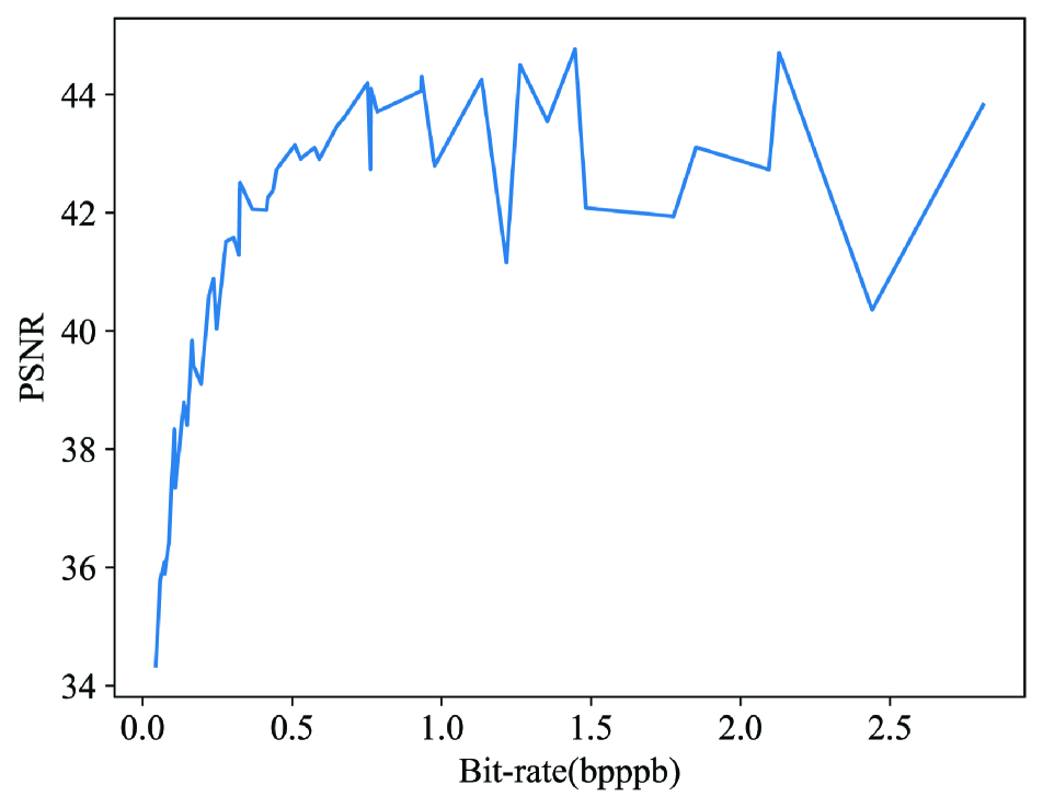
(a) Indian Pines dataset.

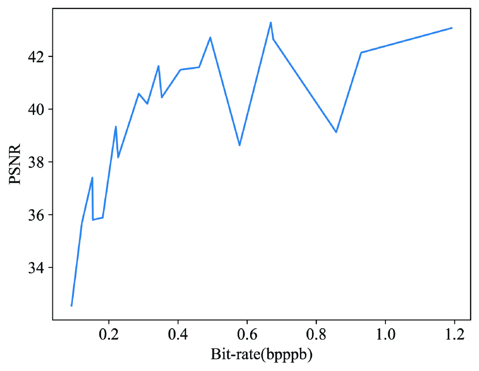
(b) Jasper Ridge dataset.

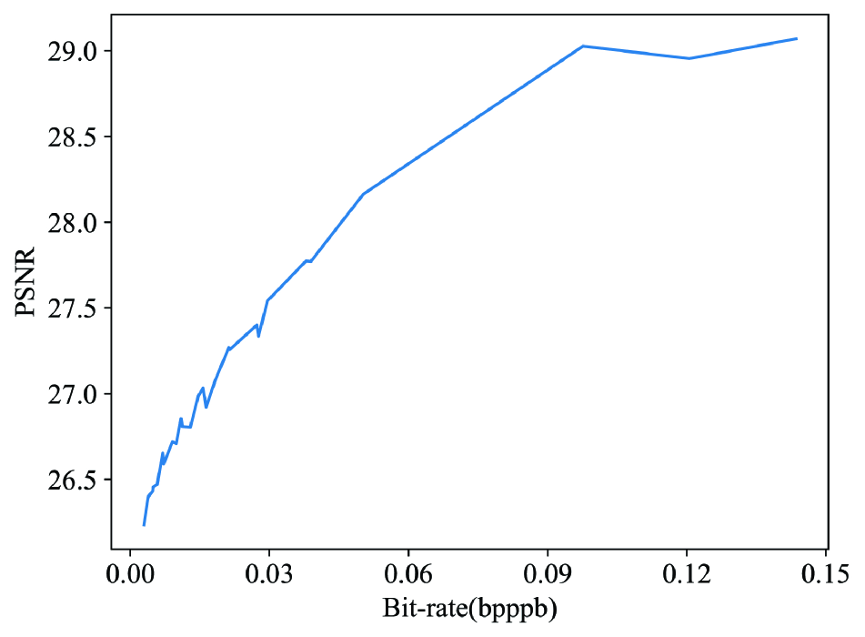
(c) Cuprite dataset.

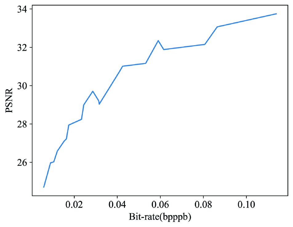
(d) Pavia University dataset.

Figure 5: Rate distortion plots on different datasets.

3.4 Datasets

We perform experiments on Indian Pines, Cuprite, Jasper Ridge, and Pavia University datasets. The AVIRIS instrument gathered the Indian Pines, Cuprite, and Jasper Ridge datasets. With the spatial dimensions in the face and the spectral dimension in the depth, respectively, the hyperspectral imaging sensors give a three-dimensional data structure known as a data cube. Figure 3 is a cube image taken by the AVIRIS satellite of the Jet Propulsion Laboratory (JPL) above Moffett Field in California. Figure 3’s false-color image on top of the cube depicts a complex structure in the water and evaporation ponds to the right. On the cube’s top, you can also see the Moffett Field airport.

The AVIRIS sensor gathers information from geometrically coherent spectroradiometric data that can be used to characterize the Earth’s surface and atmosphere. The studies of oceanography, environmental science, snow hydrology, geology, volcanology, soil and land management, atmospheric and aerosol studies, agriculture, and limnology can all benefit from the use of these data. Applications for assessing and monitoring environmental risks such as toxic waste, oil spills, and air, land, and water pollution are currently being developed. The observations can be transformed to ground reflectance data, which can subsequently be utilized for quantitative assessment of surface features, with the required calibration and adjustment for atmospheric factors.

3.4.1 Indian Pines

The Indian Pines dataset, which has 145 by 145 pixels and 16 ground-truth classes, was collected by the AVIRIS instrument in 1992. It was obtained in NW Indiana over a mixed agricultural and wooded area. There are 220 channels in this image. The Indian Pines setting is made up primarily of agriculture, with the remaining third being either forest or other types of perennial forest vegetation. Along with some low-density homes, other built objects, and minor roads, there are two significant dual-lane motorways, a rail line, and other built objects. Figure 4(a) shows an image of this dataset.

3.4.2 Jasper Ridge

One well-known hyperspectral image is Jasper Ridge. The Jet Propulsion Laboratory (JPL) captured it using the AVIRIS (Airborne Visible/Infrared Imaging Spectrometer) sensor. Its dimensions are 512 by 614 pixels. A total of 224 electromagnetic bands between 380 nm and 2,500 nm are recorded for each pixel. Figure 4(b) shows an image of this dataset.

3.4.3 Pavia University

The Pavia University dataset was captured by the ROSIS-03 aerial instrument above the Pavia University in Italy. The flight above Pavia, Italy, was conducted by the German Aerospace Centre (the German Aerospace Agency) as part of the HySens project, which is run and funded by the European Union. For Pavia Centre and Pavia University, there are 102 and 103 spectral bands, respectively. Pavia Centre is 1096 by 1096 pixel image, whereas Pavia University is 610 by 610 pixels. The Pavia University data set includes several classes, such as trees, asphalt, bitumen, gravel, metal sheet, shadow, bricks, meadow, and dirt, and it belongs to the Engineering School at the University of Pavia. Figure 4(c) shows an image of this dataset.

3.4.4 Cuprite

The Cuprite dataset covers the Cuprite in Las Vegas, Nevada, United States. There are 224 channels with wavelengths between 370 and 2480 nm. Figure 4(d) shows an image of this dataset.

(a) Jasper Ridge compression comparison plot. Our methods are compared with JPEG, JPEG2000, and PCA-DCT and outperform those benchmarks.

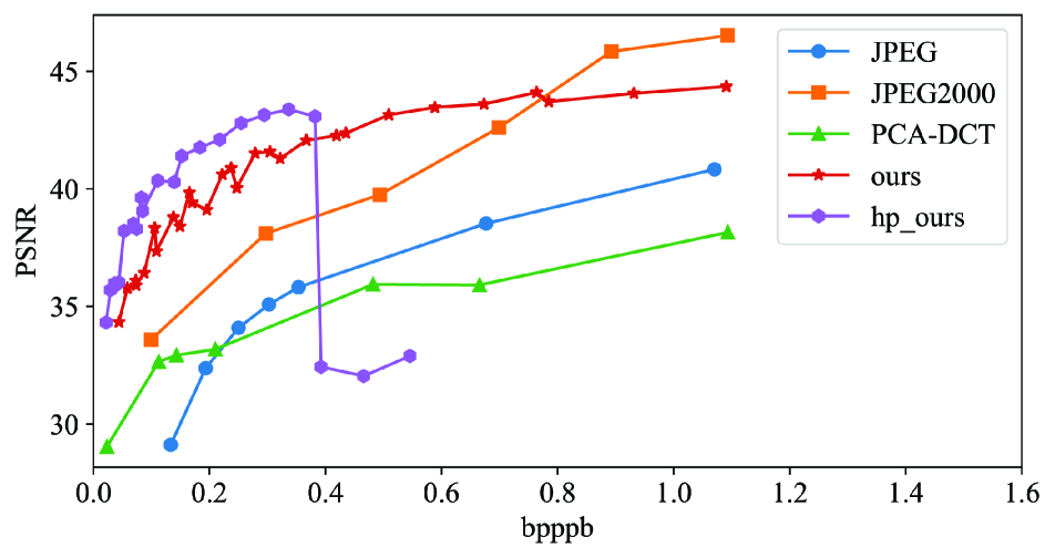
(b) Indian Pines compression comparison plot. Our methods are compared with JPEG, JPEG2000, and PCA-DCT and outperform those benchmarks in full precision.

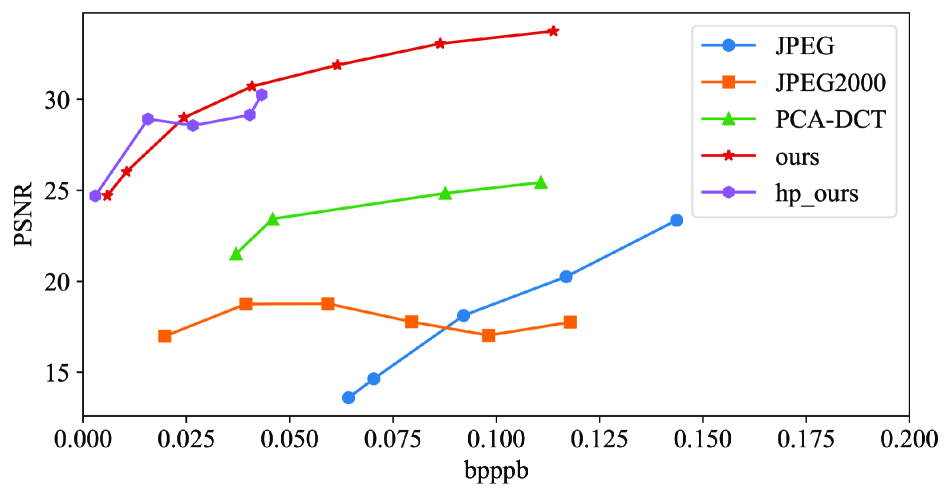
(c) Pavia University compression comparison plot. Our methods are compared with JPEG, JPEG2000, and PCA-DCT and outperform those benchmarks.

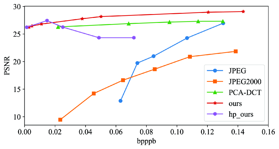
(d) Cuprite compression comparison plot. Our methods are compared with JPEG, JPEG2000, and PCA-DCT and outperform JPEG and JPEG2000 at every bit-rates and PCA-DCT at low bitrates.

Figure 6: Compression comparison plot for different datasets.

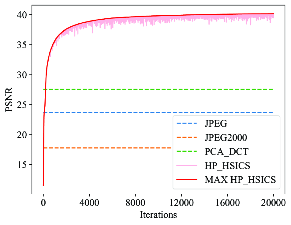
(a) Model training on Jasper Ridge dataset at 0.15 bpppb. Our method outperforms JPEG, JPEG2000, and PCA-DCT methods after some iterations and continues improving beyond that.

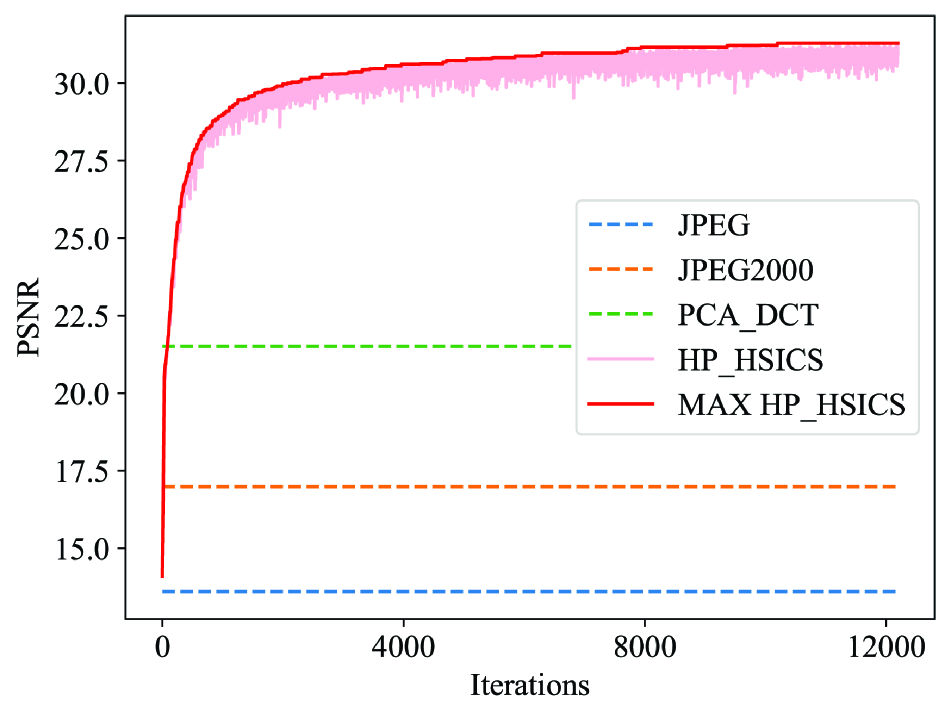
(b) Model training on Pavia University dataset at 0.025 bpppb. Our method outperforms JPEG, JPEG2000, and PCA-DCT methods after some iterations and continues improving beyond that.

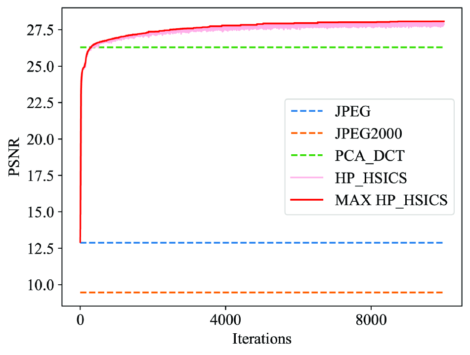
(c) Model training on Cuprite dataset at 0.02 bpppb. Our method outperforms JPEG, JPEG2000, and PCA-DCT methods after some iterations and continues improving beyond that.

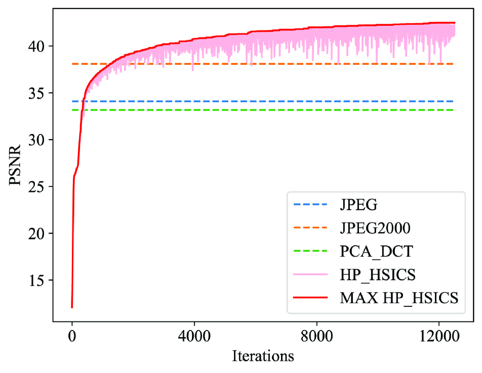
(d) Model training on Indian Pines dataset at 0.2 bpppb. Our method outperforms JPEG, JPEG2000, and PCA-DCT methods after some iterations and continues improving beyond that.

Figure 7: Model training on different datasets

4 Experiments

We compare our model against some benchmark encoders, such as JPEG [23, 44], PCA-DCT [38], and JPEG2000 [14]. JPEG 2000 uses the JPEG 2000 image compression standard and coding method to treat each band separately and encode each band independently. JPEG uses the same way to handle each band, but it uses the JPEG standard instead. PCA-DCT employs an orthogonal transformation to reconstruct a hyperspectral image into a lower-dimensional image. The first few PCs are often used, while the other components are usually discarded after compression. The PCA-DCT-based method alters the HS image’s physical composition by choosing fewer principal components. As a result, PCA-DCT was unable to achieve a higher PSNR. However, by evaluating the human vision system, PCA can still produce images with a respectable level of quality. It has been extensively utilized for HS image lossy compression uses throughout various application fields. We choose those encoders for comparison primarily because they are all known and reliable benchmark encoders.

We first identify valid depth and width configurations for the MLPs representing an image to select the optimum model designs for a particular parameter budget (measured in bits per pixel per band, or bpppb). The parameter bpppb is calculated as follows:

$$bpppb=\frac{\#parameters\times(bits\ per\ parameter)}{\#pixels\times\#bands}.$$ (4)

The optimum architecture is then chosen by doing a hyperparameter search on all viable designs and learning rates on a single image. Each image in the dataset is used to train the final model, which is then downscaled to 16-bit precision (for model compression purposes). We observe that after training, reducing the precision of weights from 32 to 16 bits caused essentially no increase in distortion, but reducing them further to 8 bits caused a large rise in distortion, outweighing the advantage of reducing the bpppb.

Peak signal-to-noise ratio (PSNR) metrics are used in the experiments to compare the accuracy of our model to JPEG, JPEG2000, and PCA-DCT. A key component of compression methods is image quality, which is determined by PSNR. The peak signal-to-noise ratio between two images is calculated using the PSNR, expressed in decibels. To contrast the level of quality of an original image compared to one that has been compressed, we utilize this ratio. As PSNR rises, the quality of the compressed or rebuilt image also rises. The efficiency of image compression is compared using the MSE and PSNR. While PSNR is a measure of the peak error, MSE is the cumulative squared error between the original and compressed image. The error decreases as the MSE value decreases. Using the following equation, we first determine the mean-squared error:

$$MSE=\frac{\Sigma_{M,N}(I_{1}(m,n)-I_{2}(m,n))^{2}}{M\times N},$$ (5)

where M and N in the previous equation stand for the input images’ respective rows and columns. The PSNR is then calculated using the following equation:

$$PSNR=10\ log_{10}\left(\frac{R^{2}}{MSE}\right),$$ (6)

where R is the largest variation in the input image in the previous equation. For instance, R is 1 if the input image is of the double-precision floating-point data. R is 255, for instance, if the data is an 8-bit unsigned integer.

Figure 5(a) for the Indian Pines dataset illustrates the outcomes of this technique for various bpppb values. As can be observed, raising the bpppb level will raise the compression quality, as determined by PSNR. We did these experiments for the other datasets, Jasper Ridge in Figure 5(b), Cuprite in figure 5(c), and Pavia University in figure 5(d), and as can be seen, the results are the same as we discussed.

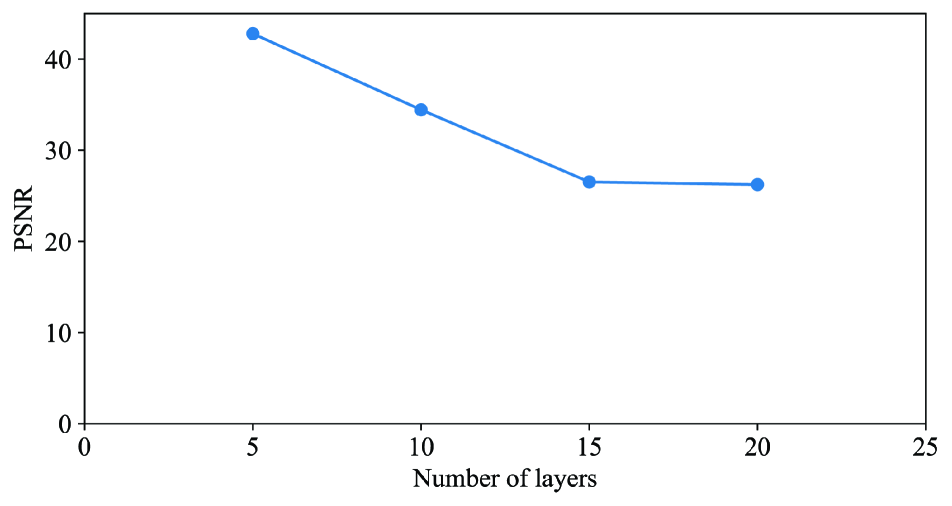
(a) Indian Pines dataset

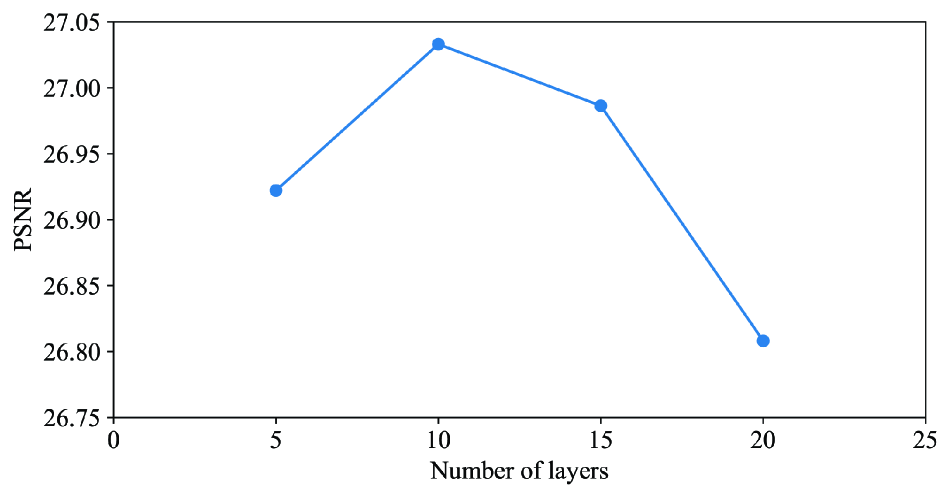
(b) Cuprite dataset

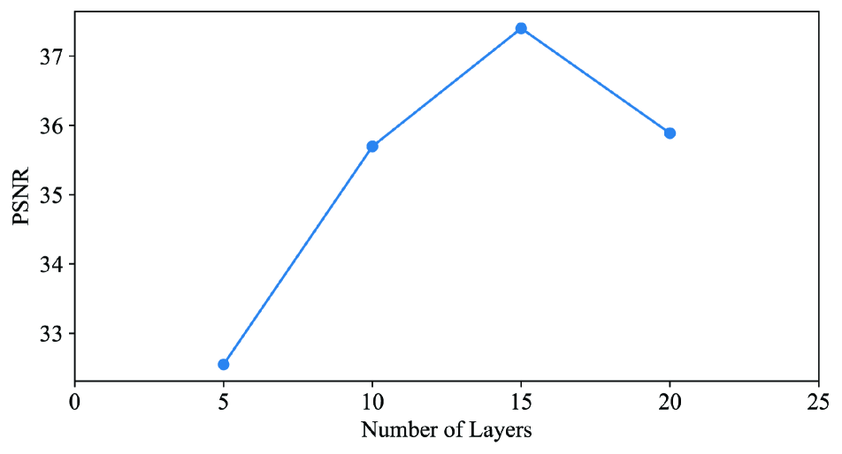
(c) Jasper Ridge dataset

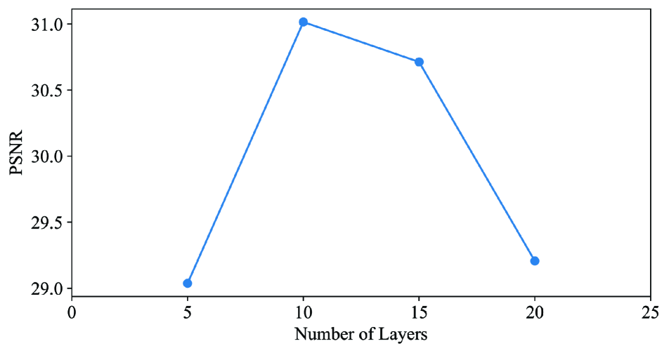
(d) Pavia University dataset

Figure 8: The performance of various valid architectures for different datasets.

4.1 Comparison with State-of-the-Art

As mentioned before, we compare our method against some benchmarks. Figure 6(a) shows this comparison for the Jasper Ridge dataset. We show the PSNRs achieved in different bpppbs for our method in two ways. We have the results with full precision (without using entropy coding), shown with HSICS; we also convert them to half-precision (using entropy coding), shown with HP_HSICS. We then compare these results with JPEG, JPEG2000, and PCA-DCT methods. As can be seen, our method outperforms JPEG, JPEG2000, and PCA-DCT at every bpppb that we do experiments with. We also conducted another experiment on Indian Pines datasets and compared its results with JPEG2000, JPEG, and PCA-DCT. As can be seen in figure 6(b), our method in full precision outperforms all other methods in this comparison at every bit-rates in bpppbs, but in half-precision, it just outperforms other methods in low bit rates (lower than 0.4 bpppb). Figures 6(c) and 6(d) shows this comparison for Pavia University and Cuprite datasets, respectively. As can be seen, our methods outperform JPEG, JPEG2000, and PCA-DCT for the experiments on the Pavia University dataset in 6(c). Figure 6(d) shows that our method outperforms JPEG, JPEG2000, and PCA-DCT, but when we want to compare the results of the half-precision method with the benchmarks, we can see that it outperforms JPEG and JPEG2000 at every bit-rates and PCA-DCT at bitrates lower than 0.02 bpppb.

Our approach does not need a decoder during testing, in contrast to the majority of previous neural data compression algorithms. In fact, the decoder model is enormous even though the latent code representing the compressed image in such systems is small. As a result, the decoding device also needs a lot of memory. In our situation, the decoder side memory requirements are orders of magnitude fewer because we only need the weights of a very small MLP. We show an example of the overfitting procedure in Figures 7(a), 7(b), 7(c), and 7(d). This experiment has been done on Jasper Ridge at 0.15 bpppb, Pavia University at 0.025 bpppb, Cuprite at 0.02 bpppb, and Indian Pines at 0.2 bpppb. We compare our model with JPEG, JPEG2000, and PCA-DCT methods. As can be seen, our method outperforms JPEG, JPEG2000, and PCA-DCT methods after some iterations and continues improving beyond that. While the optimization can be noisy, we simply save the model with the best PSNR. We just store the model with the best PSNR, given the fact that optimization can be noisy.

4.2 Experimental Details

In Figures 8(a), 8(b), 8(c), and 8(d), we show the performance of various valid architectures of size 0.2 bpppb for Indian Pines dataset, 0.01 bpppb for Cuprite dataset, 0.1 bpppb for Jasper Ridge dataset, and 0.03 bpppb for Pavia University dataset, respectively. As can be observed, the design choice affects the compression quality, with different optimal architectures for various bpppb values. In the following, we will explain the experimental detail of this work.

Adam was used to training all models. We employed MLPs with output dimensions related to the amount of dataset image bands and two input dimensions (equivalent to (x, y) coordinates). Except for the final layer, we used sine non-linearities and the initialization method given in [49]. A learning rate of 2e-4 was employed. In figures 9, 10, 11, 12, we include qualitative results comparing the compression artifacts from our proposed method and the original image on the Cuprite, Indian Pines, Jasper Ridge, and Pavia University datasets, respectively.

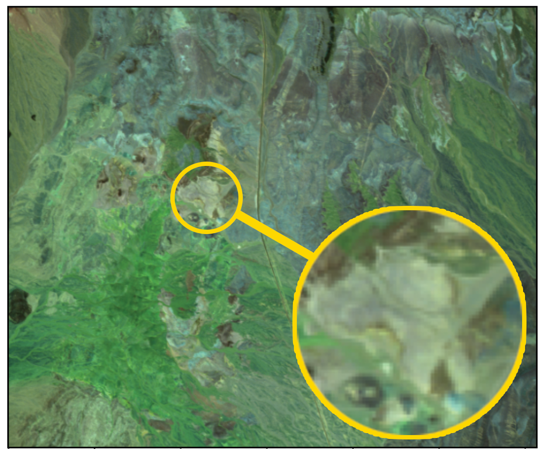
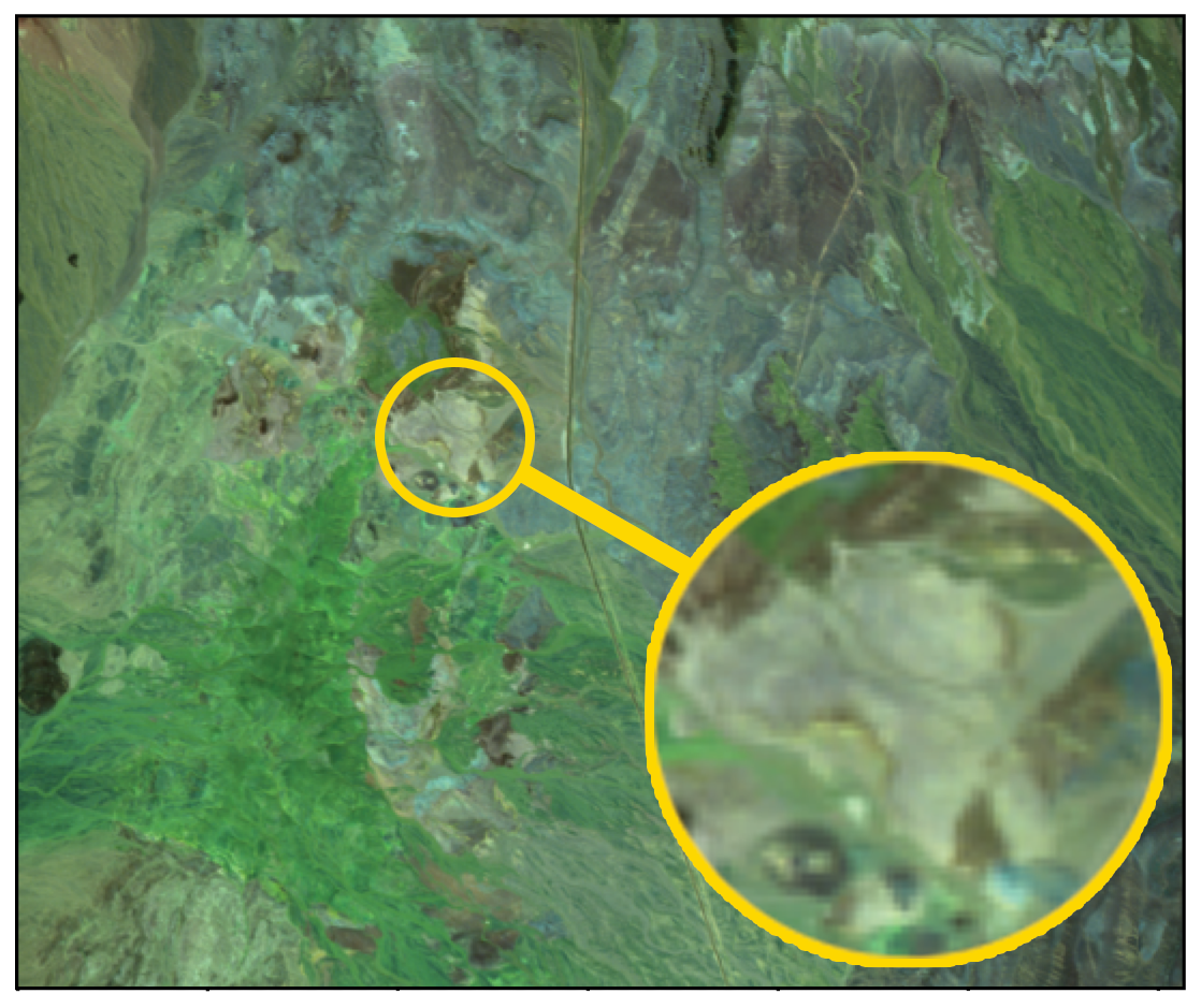
Figure 9: Cuprite original image in the left and the reconstructed image in the right.

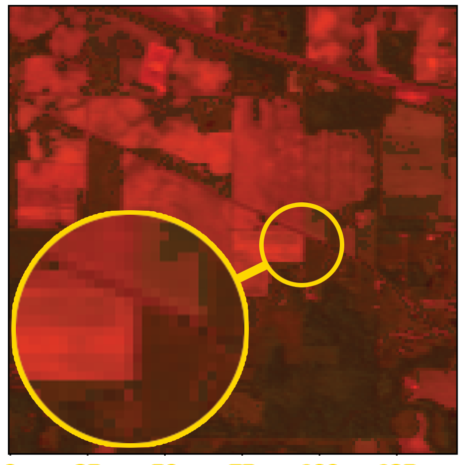
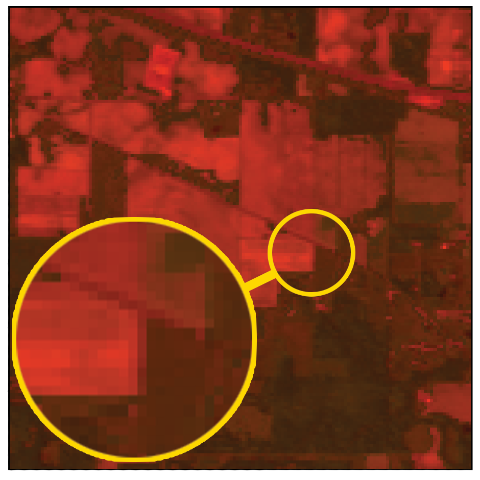
Figure 10: Indian Pines original image in the left and the reconstructed image in the right.

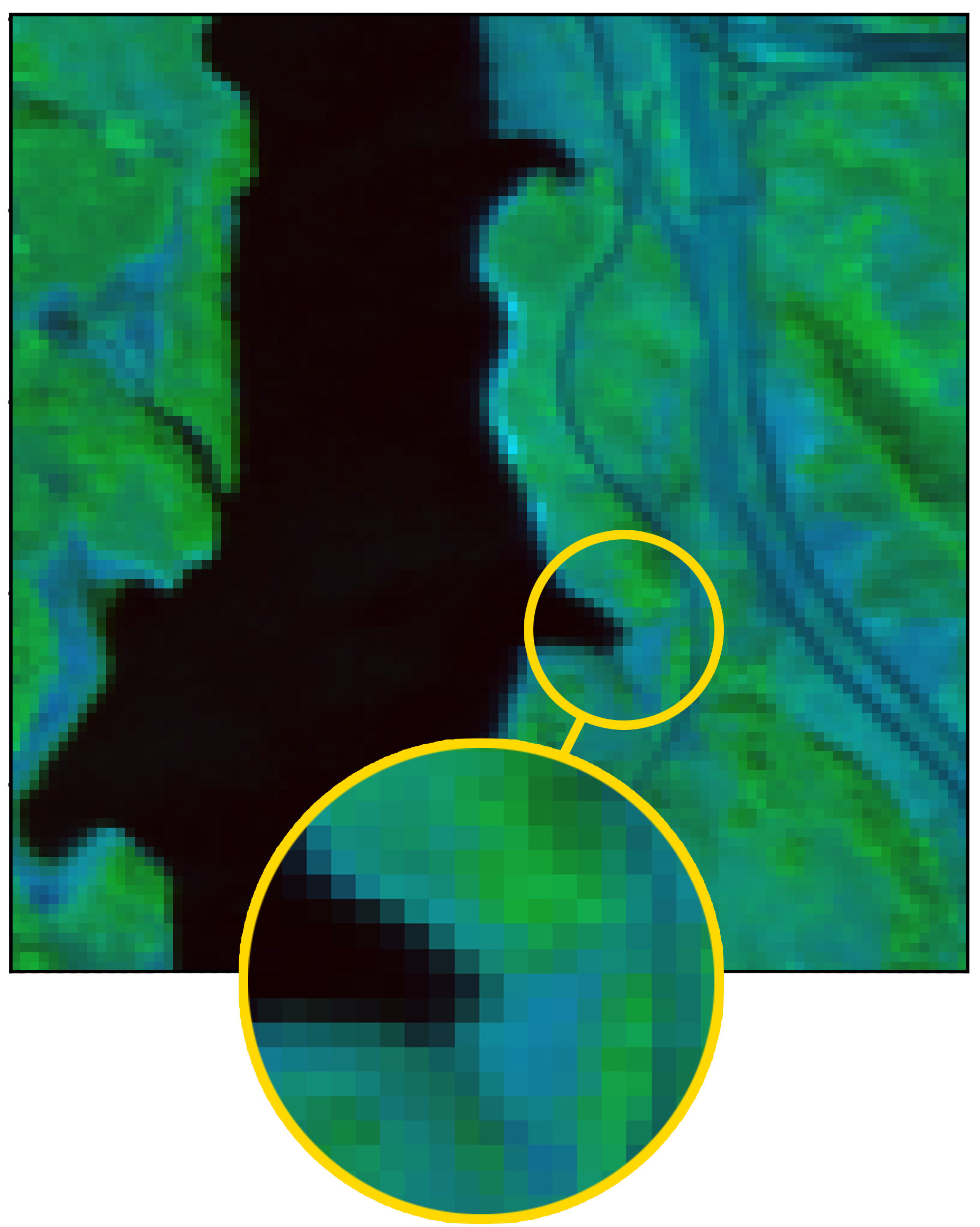
Figure 11: Jasper Ridge original image in the left and the reconstructed image in the right.

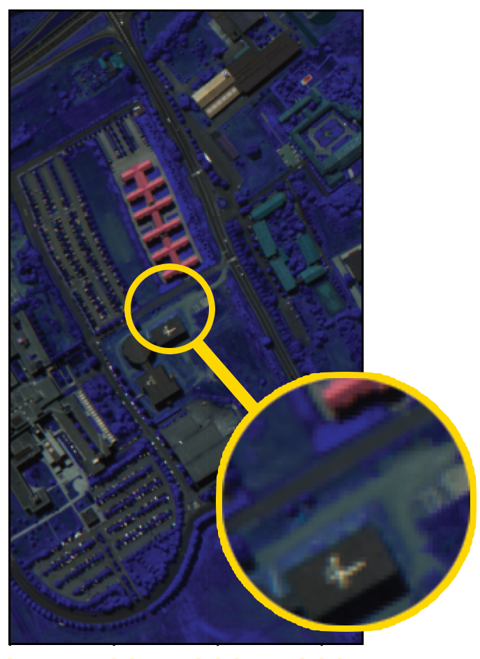
Figure 12: Pavia University original image in the left and the reconstructed image in the right.

5 Conclusion

In this work, we employ implicit neural representation to compress hyperspectral images by using neural networks to map pixel locations to band values and store the weights of the generated networks. We then assess the MLP at each pixel position to decode the image. Through experiments, we demonstrated that this method can outperform JPEG, JPEG2000, and PCA-DCT at low bit rates. For future work, we want to use meta-learned base networks, a new method for neural image compression, and then add PCA to that method to improve the results.

References

- [1] Autoencoders, minimum description length, and helmholtz free energy. In Advances in neural information processing systems, pages 3–10, 1994.
- [2] Elhadi Adam, Onisimo Mutanga, and Denis Rugege. Multispectral and hyperspectral remote sensing for identification and mapping of wetland vegetation: a review. Wetlands Ecology and Management, 18(3):281–296, 2010.
- [3] Martin A Afromowitz, James B Callis, David M Heimbach, Larry A DeSoto, and Mary K Norton. Multispectral imaging of burn wounds. In Medical Imaging II, volume 914, pages 500–504. SPIE, 1988.
- [4] A. Alemi, B. Poole, I. Fischer, J. Dillon, R.A. Saurous, and K. Murphy. Fixing a broken elbo. In Proc. 35th International Conference on Machine Learning, volume 80, pages 159–168, 2018.
- [5] J. Balle’, V. Laparra, and E.P. Simoncelli. End-to-end optimized image compression. In Proc. International Conference on Learning Representations (ICLR), June 2017.
- [6] Johannes Ballé, David Minnen, Saurabh Singh, Sung Jin Hwang, and Nick Johnston. Variational image compression with a scale hyperprior. arXiv preprint arXiv:1802.01436, 2018.
- [7] Ian Blanes and Joan Serra-Sagristà. Cost and scalability improvements to the karhunen–loêve transform for remote-sensing image coding. IEEE Transactions on Geoscience and Remote Sensing, 48(7):2854–2863, 2010.
- [8] Joaquim Campos, Simon Meierhans, Abdelaziz Djelouah, and Christopher Schroers. Content adaptive optimization for neural image compression. arXiv preprint arXiv:1906.01223, 2019.
- [9] Oscar Carrasco, Richard B Gomez, Arun Chainani, and William E Roper. Hyperspectral imaging applied to medical diagnoses and food safety. In Geo-Spatial and Temporal Image and Data Exploitation III, volume 5097, pages 215–221. SPIE, 2003.
- [10] C. I. Chang. Hyperspectral Data Processing: Algorithm Design and Analysis. Wiley, 2013.
- [11] Zhiqin Chen and Hao Zhang. Learning implicit fields for generative shape modeling. In Proceedings of the IEEE/CVF Conference on Computer Vision and Pattern Recognition, pages 5939–5948, 2019.
- [12] Roger N Clark and Gregg A Swayze. Mapping minerals, amorphous materials, environmental materials, vegetation, water, ice and snow, and other materials: the usgs tricorder algorithm. In JPL, Summaries of the Fifth Annual JPL Airborne Earth Science Workshop. Volume 1: AVIRIS Workshop, 1995.
- [13] Chris Cremer, Xuechen Li, and David Duvenaud. Inference suboptimality in variational autoencoders. In International Conference on Machine Learning, pages 1078–1086. PMLR, 2018.
- [14] Qian Du and James E Fowler. Hyperspectral image compression using jpeg2000 and principal component analysis. IEEE Geoscience and Remote sensing letters, 4(2):201–205, 2007.
- [15] Qian Du and James E Fowler. Hyperspectral image compression using jpeg2000 and principal component analysis. IEEE Geoscience and Remote sensing letters, 4(2):201–205, 2007.
- [16] Emilien Dupont, Adam Goliński, Milad Alizadeh, Yee Whye Teh, and Arnaud Doucet. Coin: Compression with implicit neural representations. arXiv preprint arXiv:2103.03123, 2021.
- [17] Gerda J Edelman, Edurne Gaston, Ton G Van Leeuwen, PJ Cullen, and Maurice CG Aalders. Hyperspectral imaging for non-contact analysis of forensic traces. Forensic science international, 223(1-3):28–39, 2012.
- [18] Yao-Ze Feng and Da-Wen Sun. Application of hyperspectral imaging in food safety inspection and control: a review. Critical reviews in food science and nutrition, 52(11):1039–1058, 2012.
- [19] Christian Fischer and Ioanna Kakoulli. Multispectral and hyperspectral imaging technologies in conservation: current research and potential applications. Studies in Conservation, 51(sup1):3–16, 2006.
- [20] Pedram Ghamisi, Naoto Yokoya, Jun Li, Wenzhi Liao, Sicong Liu, Javier Plaza, Behnood Rasti, and Antonio Plaza. Advances in hyperspectral image and signal processing: A comprehensive overview of the state of the art. IEEE Geoscience and Remote Sensing Magazine, 5(4):37–78, 2017.
- [21] Alexander FH Goetz, Gregg Vane, Jerry E Solomon, and Barrett N Rock. Imaging spectrometry for earth remote sensing. science, 228(4704):1147–1153, 1985.
- [22] Jorge González-Conejero, Joan Bartrina-Rapesta, and Joan Serra-Sagrista. Jpeg2000 encoding of remote sensing multispectral images with no-data regions. IEEE Geoscience and Remote Sensing Letters, 7(2):251–255, 2009.
- [23] Walter F Good, Glenn S Maitz, and David Gur. Joint photographic experts group (jpeg) compatible data compression of mammograms. Journal of Digital Imaging, 7(3):123–132, 1994.
- [24] Megandhren Govender, Kershani Chetty, and Hartley Bulcock. A review of hyperspectral remote sensing and its application in vegetation and water resource studies. Water Sa, 33(2):145–151, 2007.
- [25] Aoife A Gowen, Colm P O’Donnell, Patrick J Cullen, Gérard Downey, and Jesus M Frias. Hyperspectral imaging–an emerging process analytical tool for food quality and safety control. Trends in food science & technology, 18(12):590–598, 2007.
- [26] Tiansheng Guo, Jing Wang, Ze Cui, Yihui Feng, Yunying Ge, and Bo Bai. Variable rate image compression with content adaptive optimization. In Proceedings of the IEEE/CVF Conference on Computer Vision and Pattern Recognition Workshops, pages 122–123, 2020.
- [27] Devon Hjelm, Russ R Salakhutdinov, Kyunghyun Cho, Nebojsa Jojic, Vince Calhoun, and Junyoung Chung. Iterative refinement of the approximate posterior for directed belief networks. Advances in neural information processing systems, 29, 2016.
- [28] Yoon Kim, Sam Wiseman, Andrew Miller, David Sontag, and Alexander Rush. Semi-amortized variational autoencoders. In International Conference on Machine Learning, pages 2678–2687. PMLR, 2018.
- [29] Rahul Krishnan, Dawen Liang, and Matthew Hoffman. On the challenges of learning with inference networks on sparse, high-dimensional data. In International conference on artificial intelligence and statistics, pages 143–151. PMLR, 2018.
- [30] Jaana Kuula, Ilkka Pölönen, Hannu-Heikki Puupponen, Tuomas Selander, Tapani Reinikainen, Tapani Kalenius, and Heikki Saari. Using vis/nir and ir spectral cameras for detecting and separating crime scene details. In Sensors, and Command, Control, Communications, and Intelligence (C3I) Technologies for Homeland Security and Homeland Defense XI, volume 8359, page 83590P. International Society for Optics and Photonics, 2012.
- [31] MCJJ L EH. Lightness and retinex theory. J. Opt. Soc. Am., 61(1):1–11, 1971.
- [32] Jooyoung Lee, Seunghyun Cho, and Seung-Kwon Beack. Context-adaptive entropy model for end-to-end optimized image compression. arXiv preprint arXiv:1809.10452, 2018.
- [33] Haida Liang. Advances in multispectral and hyperspectral imaging for archaeology and art conservation. Applied Physics A, 106(2):309–323, 2012.
- [34] Joe Marino, Yisong Yue, and Stephan Mandt. Iterative amortized inference. In International Conference on Machine Learning, pages 3403–3412. PMLR, 2018.
- [35] J. Mielikainen and B. Huang. Lossless compression of hyperspectral images using clustered linear prediction with adaptive prediction length. IEEE Geosci. Remote Sens. Lett., (9):1118–1121, 2012.
- [36] Ben Mildenhall, Pratul P Srinivasan, Matthew Tancik, Jonathan T Barron, Ravi Ramamoorthi, and Ren Ng. Nerf: Representing scenes as neural radiance fields for view synthesis. In European conference on computer vision, pages 405–421. Springer, 2020.
- [37] David Minnen, Johannes Ballé, and George D Toderici. Joint autoregressive and hierarchical priors for learned image compression. Advances in neural information processing systems, 31, 2018.
- [38] Yongjian Nian, Yu Liu, and Zhen Ye. Pairwise klt-based compression for multispectral images. Sensing and Imaging, 17(1):1–15, 2016.
- [39] Michael Niemeyer, Lars Mescheder, Michael Oechsle, and Andreas Geiger. Occupancy flow: 4d reconstruction by learning particle dynamics. In Proceedings of the IEEE/CVF international conference on computer vision, pages 5379–5389, 2019.
- [40] N. R. Mat Noor and T. Vladimirova. Investigation into lossless hyperspectral image compression for satellite remote sensing. International Journal of Remote Sensing, 34:5072–5104, 2013.
- [41] R Padoan, TA Steemers, M Klein, B Aalderink, and G De Bruin. Quantitative hyperspectral imaging of historical documents: technique and applications. Art Proceedings, pages 25–30, 2008.
- [42] Jeong Joon Park, Peter Florence, Julian Straub, Richard Newcombe, and Steven Lovegrove. Deepsdf: Learning continuous signed distance functions for shape representation. In Proceedings of the IEEE/CVF Conference on Computer Vision and Pattern Recognition, pages 165–174, 2019.
- [43] Barbara Penna, Tammam Tillo, Enrico Magli, and Gabriella Olmo. Transform coding techniques for lossy hyperspectral data compression. IEEE Transactions on Geoscience and Remote Sensing, 45(5):1408–1421, 2007.
- [44] Tong Qiao, Jinchang Ren, Meijun Sun, Jiangbin Zheng, and Stephen Marshall. Effective compression of hyperspectral imagery using an improved 3d dct approach for land-cover analysis in remote-sensing applications. International Journal of Remote Sensing, 35(20):7316–7337, 2014.
- [45] Tong Qiao, Jinchang Ren, Meijun Sun, Jiangbin Zheng, and Stephen Marshall. Effective compression of hyperspectral imagery using an improved 3d dct approach for land-cover analysis in remote-sensing applications. International Journal of Remote Sensing, 35(20):7316–7337, 2014.
- [46] Behnood Rasti, Johannes R Sveinsson, Magnus O Ulfarsson, and Jon Atli Benediktsson. Hyperspectral image denoising using 3d wavelets. In 2012 IEEE International Geoscience and Remote Sensing Symposium, pages 1349–1352. IEEE, 2012.
- [47] Basri Ronen, David Jacobs, Yoni Kasten, and Shira Kritchman. The convergence rate of neural networks for learned functions of different frequencies. Advances in Neural Information Processing Systems, 32, 2019.
- [48] Rebecca L Schuler, Paul E Kish, and Cara A Plese. Preliminary observations on the ability of hyperspectral imaging to provide detection and visualization of bloodstain patterns on black fabrics. Journal of forensic sciences, 57(6):1562–1569, 2012.
- [49] Vincent Sitzmann, Julien Martel, Alexander Bergman, David Lindell, and Gordon Wetzstein. Implicit neural representations with periodic activation functions. Advances in Neural Information Processing Systems, 33:7462–7473, 2020.
- [50] Kenneth O Stanley. Compositional pattern producing networks: A novel abstraction of development. Genetic programming and evolvable machines, 8(2):131–162, 2007.
- [51] Matthew Tancik, Pratul Srinivasan, Ben Mildenhall, Sara Fridovich-Keil, Nithin Raghavan, Utkarsh Singhal, Ravi Ramamoorthi, Jonathan Barron, and Ren Ng. Fourier features let networks learn high frequency functions in low dimensional domains. Advances in Neural Information Processing Systems, 33:7537–7547, 2020.
- [52] Ties van Rozendaal, Iris AM Huijben, and Taco S Cohen. Overfitting for fun and profit: Instance-adaptive data compression. arXiv preprint arXiv:2101.08687, 2021.
- [53] Lei Wang, Jiaji Wu, Licheng Jiao, and Guangming Shi. Lossy-to-lossless hyperspectral image compression based on multiplierless reversible integer tdlt/klt. IEEE Geoscience and remote sensing letters, 6(3):587–591, 2009.
- [54] Yibo Yang, Robert Bamler, and Stephan Mandt. Improving inference for neural image compression. Advances in Neural Information Processing Systems, 33:573–584, 2020.
- [55] L. Zhang, L. Zhang, D. Tao, X. Huang, and B. Du. Compression of hyperspectral remote sensing images by tensor approach. Neurocomputing, (147):358–363, 2015.
- [56] Dongyu Zhao, Shiping Zhu, and Fengchao Wang. Lossy hyperspectral image compression based on intra-band prediction and inter-band fractal encoding. Computers & Electrical Engineering, 54:494–505, 2016.