Cliques in High-Dimensional Geometric Inhomogeneous Random Graphs

Abstract

A recent trend in the context of graph theory is to bring theoretical analyses closer to empirical observations, by focusing the studies on random graph models that are used to represent practical instances. There, it was observed that geometric inhomogeneous random graphs (GIRGs) yield good representations of complex real-world networks, by expressing edge probabilities as a function that depends on (heterogeneous) vertex weights and distances in some underlying geometric space that the vertices are distributed in. While most of the parameters of the model are understood well, it was unclear how the dimensionality of the ground space affects the structure of the graphs.

In this paper, we complement existing research into the dimension of geometric random graph models and the ongoing study of determining the dimensionality of real-world networks, by studying how the structure of GIRGs changes as the number of dimensions increases. We prove that, in the limit, GIRGs approach non-geometric inhomogeneous random graphs and present insights on how quickly the decay of the geometry impacts important graph structures. In particular, we study the expected number of cliques of a given size as well as the clique number and characterize phase transitions at which their behavior changes fundamentally. Finally, our insights help in better understanding previous results about the impact of the dimensionality on geometric random graphs.

1 Introduction

Networks are a powerful tool to model all kinds of processes that we interact with in our day-to-day lives. From connections between people in social networks, to the exchange of information on the internet, and on to how our brains are wired, networks are everywhere. Consequently, they have been in the focus of computer science for decades. There, one of the most fundamental techniques used to model and study networks are random graph models. Such a model defines a probability distribution over graphs, which is typically done by specifying a random experiment on how to construct the graph. By analyzing the rules of the experiment, we can then derive structural and algorithmic properties of the resulting graphs. If the results match what we observe on real-world networks, i.e., if the model represents the graphs we encounter in practice well, then we can use it to make further predictions that help us understand real graphs and utilize them more efficiently.

The quest of finding a good model starts several decades ago, with the famous Erdős-Rényi (ER) random graphs [19, 23]. There, all edges in the graph exist independently with the same probability. Due to its simplicity, this model has been studied extensively. However, because the degree distribution of the resulting graphs is rather homogeneous and they lack clustering (due to the independence of the edges), the model is not considered to yield good representations of real graphs. In fact, many networks we encounter in practice feature a degree distribution that resembles a power-law [3, 37, 38] and the clustering coefficient (the probability for two neighbors of a vertex to be adjacent) is rather high [34, 39]. To overcome these drawbacks, the initial random graph model has been adjusted in several ways.

In inhomogeneous random graphs (IRGs), often referred to as Chung-Lu random graphs, each vertex is assigned a weight and the probability for two vertices to be connected by an edge is proportional to the product of the weights [1, 11, 12]. As a result, the expected degrees of the vertices in the resulting graphs match their weight. While assigning weights that follow a power-law distribution yields graphs that are closer to the complex real-world networks, the edges are still drawn independently, leading to vanishing clustering coefficients.

A very natural approach to facilitate clustering in a graph model is to introduce an underlying geometry. This was done first in random geometric graphs (RGGs), where vertices are distributed uniformly at random in the Euclidean unit square and any two are connected by an edge if their distance lies below a certain threshold, i.e., the neighborhood of a vertex lives in a disk centered at that vertex [35]. Intuitively, two vertices that connect to a common neighbor cannot be too far away from each other, increasing the probability that they are connected by an edge themselves. In fact, random geometric graphs feature a non-vanishing clustering coefficient [13]. However, since all neighborhood disks have the same size, they all have roughly the same expected degree, again, leading to a homogeneous degree distribution.

To get a random graph model that features a heterogeneous degree distribution and clustering, the two mentioned adjustments were recently combined to obtain geometric inhomogeneous random graphs (GIRGs) [27]. There, vertices are assigned a weight and a position in some underlying geometric space and the probability for two vertices to connected increases with the product of the weights but decreases with increasing geometric distance between them. As a result, the generated graphs have a non-vanishing clustering coefficient and, with the appropriate choice of the weight sequence, they feature a power-law degree distribution. Additionally, recent empirical observations indicate that GIRGs represent real-world networks well with respect to certain structural and algorithmic properties [5].

We note that GIRGs are not the first model that exhibits a heterogeneous degree distribution and clustering. In fact, hyperbolic random graphs (HRGs) [29] feature these properties as well and have been studied extensively before (see, e.g., [7, 20, 21, 22, 25]). However, in the pursuit of finding good models to represent real-world networks, GIRGs introduce a parameter that sets them apart from prior models: the choice of the underlying geometric space and, more importantly, the dimensionality of that space.

Unfortunately, this additional parameter that sets GIRGs apart from previous models, has not gained much attention at all. In fact, it comes as a surprise that, while the underlying dimensionality of real-world networks is actively researched [2, 8, 15, 24, 30] and there is a large body of research examining the impact of the dimensionality on different homogeneous graph models [13, 17, 18] with some advancements being made on hyperbolic random graphs [40], the effects of the dimension on the structure of GIRGs have only been studied sparsely. For example, while it is known that GIRGs exhibit a clustering coefficient of $\Theta(1)$ for any fixed dimension [27], it is not known how the hidden constants scale with the dimension.

In this paper, we initiate the study of the impact of the dimensionality on GIRGs. In particular, we investigate the influence of the underlying geometry as the dimensionality increases, proving that GIRGs converge to their non-geometric counterpart (IRGs) in the limit. With our results we are able to explain seemingly disagreeing insights from prior research on the impact of dimensionality on geometric graph models. Moreover, by studying the clique structure of GIRGs and its dependence on the dimension $d$, we are able to quantify how quickly the underlying geometry vanishes. In the following, we discuss our results in greater detail.

1.1 (Geometric) Inhomogeneous Random Graphs

Before stating our results in greater detail, let us recall the definitions of the two graph models we mainly work with throughout the paper.

Inhomogeneous Random Graphs (IRGs).

The model of inhomogeneous random graphs was introduced by Chung and Lu [1, 11, 12] and is a natural generalization of the Erdős-Rényi model. Starting with a vertex set $V$ of $n$ vertices, each $v\in V$ is assigned a weight $w_{v}$. Each edge $\{u,v\}\in\binom{V}{2}$ is then independently present with probability

$$\mathrm{Pr}\left[u\sim v\right]=\min\left\{1,\frac{\lambda w_{u}w_{v}}{n}\right\},$$

for some constant $\lambda>0$ controlling the average degree of the resulting graph. Note that assigning the same weight to all vertices yields the same connection probability as in Erdős-Rényi random graphs. For the sake of simplicity, we define $\kappa_{uv}=\min\{\lambda w_{u}w_{v},n\}$ such that $\mathrm{Pr}\left[u\sim v\right]=\kappa_{uv}/n$. Additionally, for a set of vertices $U_{k}=\{v_{1},\ldots,v_{k}\}$ with weights $w_{1},\ldots,w_{k}$, we introduce the shorthand notation $\kappa_{ij}=\kappa_{v_{i}v_{j}}$ and write $\{\kappa\}^{(k)}=\{\kappa_{ij}\mid 1\leq i<j\leq k\}$.

Throughout the paper, we mainly focus inhomogeneous random graphs that feature a power-law degree distribution in expectation, which is obtained by sampling the weights accordingly. More precisely, for each $v\in V$, we sample a weight $w_{v}$ from the Pareto distribution $\mathcal{P}$ with parameters $1-\beta,w_{0}$ and distribution function

$$\mathrm{Pr}\left[w_{v}\leq x\right]=1-\left(\frac{x}{w_{0}}\right)^{1-\beta}.$$

Then the density of $w_{v}$ is $\rho_{w_{v}}(x)=\frac{\beta-1}{w_{0}^{1-\beta}}x^{-\beta}$. Here, $w_{0}>0$ is a constant that represents a lower bound on the weights in the graph and $\beta$ denotes the power-law exponent of the resulting degree distribution. Throughout the paper, we assume $\beta>2$ such that a single weight has finite expectation (and thus the average degree in the graph is constant), but possibly infinite variance. We denote a graph obtained by utilizing the above weight distribution and connection probabilities with $\operatorname{IRG}(n,\beta,w_{0})$. For a fixed weight sequence $\{w\}_{1}^{n}$, we denote the corresponding graph by $\operatorname{IRG}(\{w\}_{1}^{n})$.

Geometric Inhomogeneous Random Graphs (GIRGs).

Geometric inhomogeneous random graphs are an extension of IRGs, where in addition to the weight, each vertex $v$ is also equipped with a position $\mathbf{x}_{v}$ in some geometric space and the probability for edges to form depends on their weights and the distance in the underlying space [27]. While, in its raw form, the GIRG framework is rather general, we align our paper with existing analysis on GIRGs [6, 28, 33] and consider the $d$-dimensional torus $\mathbb{T}^{d}$ equipped with $L_{\infty}$-norm as the geometric ground space. More precisely, in what we call the standard GIRG model, the positions $\mathbf{x}$ of the vertices are drawn independently and uniformly at random from $\mathbb{T}^{d}$, according to the standard Lebesgue measure. We denote the $i$-th component of $\mathbf{x}_{v}$ by $\mathbf{x}_{vi}$. Additionally, the geometric distance between two points $\mathbf{x}_{u}$ and $\mathbf{x}_{v}$, is given by

$$d(\mathbf{x}_{u},\mathbf{x}_{v})=\|\mathbf{x}_{u}-\mathbf{x}_{v}\|_{\infty}=\max_{1\leq i\leq d}\{|\mathbf{x}_{ui}-\mathbf{x}_{vi}|_{C}\},$$

where $|\cdot|_{C}$ denotes the distance on the circle, i.e,

$$|\mathbf{x}_{ui}-\mathbf{x}_{vi}|_{C}=\min\{|\mathbf{x}_{ui}-\mathbf{x}_{vi}|,1-|\mathbf{x}_{ui}-\mathbf{x}_{vi}|\}.$$

In a standard GIRG, two vertices $u\neq v$ are adjacent if and only if their distance $d(\mathbf{x}_{u},\mathbf{x}_{v})$ in the torus is less than or equal to a connection threshold $t_{uv}$, which is given by

$$t_{uv}=\frac{1}{2}\left(\frac{\lambda w_{u}w_{v}}{n}\right)^{1/d}=\left(\frac{w_{u}w_{v}}{\tau n}\right)^{1/d},$$

where $\tau=2^{d}/\lambda$. Using $L_{\infty}$ is motivated by the fact that it is the most widely used metric in the literature because it is arguably the most natural metric on the torus. In particular, it has the “nice” property that the ball of radius $r$ is a cube and “fits” entirely into $\mathbb{T}^{d}$ for all $0\leq r\leq 1$.

Note that that, as a consequence of the above choice, the marginal connection probability $\mathrm{Pr}\left[u\sim v\right]$ is the same as in the IRG model, i.e., $\mathrm{Pr}\left[u\sim v\right]=\kappa_{uv}/n$. However, while the probability that any given edge is present is the same as in the IRG model, the edges in the GIRG model are not drawn independently. We denote a graph obtained by the procedure described above with $\operatorname{GIRG}(n,\beta,w_{0},d)$. As for IRGs, we write $\operatorname{GIRG}(\{w\}_{1}^{n},d)$ when considering standard GIRGs with a fixed weight sequence $\{w\}_{1}^{n}$.

As mentioned above, the standard GIRG model is a commonly used instance of the more general GIRG framework [27]. There, different geometries and distance functions may be used. For example, instead of $L_{\infty}$-norm, any $L_{p}$-norm for $1\leq p<\infty$ may be used. Then, the distance between two vertices $u,v$ is measured as

$$\|\mathbf{x}_{u}-\mathbf{x}_{v}\|_{p}\coloneqq\begin{cases}\left(\sum_{i=1}^{d}|\mathbf{x}_{ui}-\mathbf{x}_{vi}|^{p}\right)^{1/p}&\text{if }p<\infty\\ \max_{1\leq i\leq d}\{|\mathbf{x}_{ui}-\mathbf{x}_{vi}|\}&\text{otherwise.}\end{cases}$$

With this choice, the volume (Lebesgue measure) of the ball $B_{p}(r)$ of radius $r$ under $L_{p}$-norm is equal to the probability that a vertex $u$ falls within distance at most $r$ of $v$ (if $r=o(1)$). We denote this volume by $\nu(r)$. We call the corresponding graphs standard GIRGs with any $L_{p}$-norm and note that some of our results extend to this more general model. Finally, whenever our insights consider an even broader variant of the model (e.g., variable ground spaces, distances functions, weight distributions), we say that they hold for any GIRG and mention the constraints explicitly.

1.2 Asymptotic Equivalence

Our first main observations is that large values of $d$ diminish the influence of the underlying geometry until, at some point, our model becomes strongly equivalent to its non-geometric counterpart, where edges are sampled independently of each other. We prove that the total variation distance between the distribution over all graphs of the two models tends to zero as $n$ is kept fixed and $d\rightarrow\infty$. We define the total variation distance of two probability measures $P$ and $Q$ on the measurable space $(\Omega,\mathcal{F})$ as

$$\|P,Q\|_{\text{TV}}=\sup_{A\in\mathcal{F}}|P(A)-P(B)|=\frac{1}{2}\sum_{\omega\in\Omega}|P(\omega)-Q(\omega)|,$$

where the second equality holds if $\Omega$ is countable. In our case, $\Omega$ is the set $\mathcal{G}(n)$ of all possible graphs on $n$ vertices, and $P,Q$ are distributions over these graphs. If $G_{1},G_{2}$ are two random variables mapping to $\Omega$, we refer to $\|G_{1},G_{2}\|_{\text{TV}}$ as the total variation distance of the induced probability measures by $G_{1}$ and $G_{2}$, respectively. Informally, this measures the maximum difference in the probability that any graph $G$ is sampled by $G_{1}$ and $G_{2}$.

Theorem 1.1.

Let $\mathcal{G}(n)$ be the set of all graphs with $n$ vertices, let $\{w\}_{1}^{n}$ be a weight sequence, and consider $G_{\text{IRG}}=\operatorname{IRG}(\{w\}_{1}^{n})\in\mathcal{G}(n)$ and a standard GIRG $G_{\text{GIRG}}=\operatorname{GIRG}(\{w\}_{1}^{n},d)\in\mathcal{G}(n)$ with any $L_{p}$-norm. Then,

$$\lim_{d\rightarrow\infty}\|G_{\text{GIRG}},G_{\text{IRG}}\|_{\text{TV}}=0.$$

We note that this theorem holds for arbitrary weight sequences that do not necessarily follow a power law and for arbitrary $L_{p}$-norms used to define distances in the ground space. For $p\in[1,\infty)$, the proof is based on the application of a multivariate central limit theorem [36], in a similar way as used to prove a related statement for spherical random geometric graphs (SRGGs), i.e., random geometric graphs with a hypersphere as ground space [17]. Our proof generalizes this argument to arbitrary $L_{p}$-norms and arbitrary weight sequences. For the case of $L_{\infty}$-norm, we present a proof based on the inclusion-exclusion principle and the bounds we develop in Section 4.

Remarkably, while a similar behavior was previously established for SRGGs, there exist works indicating that RGGs on the hypercube do not converge to their non-geometric counterpart [13, 18] as $d\rightarrow\infty$. We show that this apparent disagreement is due to the fact that the torus is a homogeneous space while the hypercube is not. In fact, our proof shows that GIRGs on the hypercube do converge to a non-geometric model in which edges are, however, not sampled independently. This lack of independence is because, on the hypercube, there is a positive correlation between the distances from two vertices to a given vertex, leading to a higher tendency to form clusters, as was observed experimentally [18]. Due to the homogeneous nature of the torus, the same is not true for GIRGs and the model converges to the plain IRG model with independent edges.

1.3 Clique Structure

To quantify for which dimensions $d$ the graphs in the GIRG model start to behave similar to IRGs, we investigate the number and size of cliques. Previous results on SRGGs indicate that the dimension of the underlying space heavily influences the clique structure of the model [4, 17]. However, it was not known how the size and the number of cliques depends on $d$ if we use the torus as our ground space, and how the clique structure in high-dimensions behaves for inhomogeneous weights.

We give explicit bounds on the expected number of cliques of a given size $k$, which we afterwards turn into bounds on the clique number $\omega(G)$, i.e., the size of the largest clique in the graph $G$. While the expected number of cliques in the GIRG model was previously studied by Michielan and Stegehuis [33] when the power-law exponent of the degree distribution satisfies $\beta\in(2,3)$, to the best of our knowledge, the clique number of GIRGs remains unstudied even in the case of constant (but arbitrary) dimensionality. We close this gap, reproduce the existing results, and extend them to the case $\beta\geq 3$ and the case where $d$ can grow as a function of the number of vertices $n$ in the graph. Furthermore, our bounds for the case $\beta\in(2,3)$ are more explicit and complement the work of Michielan and Stegehuis, who expressed the (rescaled) asymptotic number of cliques as converging to a non-analytically solvable integral. Furthermore, we show that the clique structure in our model eventually behaves asymptotically like that of an IRG if the dimension is sufficiently large. In summary, our main contributions are outlined in Tables 1, 2, and Table 3.

Table 1: Asymptotic behavior of the expected number of $k$-cliques. The behavior in the first column is the same as in hyperbolic random graphs [7], and the behavior in the third column is the same as in the IRG model [14]. Results marked with * were previously known for constant $k$ [33].

$\mathbb{E}\left[K_{k}\right]$ for $k\geq 4$
	$d=\Theta(1)$	$d=o(\log(n))$	$d=\omega(\log(n))$
$2<\beta<3,k>\frac{2}{3-\beta}$	$n^{\frac{k}{2}(3-\beta)}\Theta(k)^{-k}$*	$n^{\frac{k}{2}(3-\beta)}\Theta(k)^{-k}$	$n^{\frac{k}{2}(3-\beta)}\Theta(k)^{-k}$
$2<\beta<3,k<\frac{2}{3-\beta}$	$n\Theta(k)^{-k}$*	$ne^{-\Theta(1)dk}\Theta(k)^{-k}$	$n^{\frac{k}{2}(3-\beta)}\Theta(k)^{-k}$
$\beta>3$	$n\Theta(k)^{-k}$	$ne^{-\Theta(1)dk}\Theta(k)^{-k}$	$o(1)$

We observe that the structure of the cliques undergoes three phase transitions in the size of the cliques $k$, the dimension $d$, and the power-law exponent $\beta$.

Transition in $k$.

When $\beta\in(2,3)$ and $d\in o(\log(n))$, the first transition is at $k=\frac{2}{3-\beta}$, as was previously observed for hyperbolic random graphs [7] and for GIRGs of constant dimensionality [33]. The latter work explains this behavior by showing that for $k<\frac{2}{3-\beta}$, the number of cliques is strongly dominated by “geometric” cliques forming among vertices whose distance is of order $n^{-1/d}$ regardless of their weight. For $k>\frac{2}{3-\beta}$, on the other hand, the number of cliques is dominated by “non-geometric” cliques forming among vertices with weights in the order of $\sqrt{n}$. This behavior is in contrast to the behavior of cliques in the IRG model, where this phase transition does not exist and where the expected number of $k$ cliques is $\Theta\left(n^{\frac{k}{2}(3-\beta)}\right)$ for all $k\geq 3$ (if $\beta\in(2,3)$) [14].

Transition in $d$.

Still assuming $\beta\in(2,3)$, the second phase transition occurs as $d$ becomes superlogarithmic. More precisely, we show that in the high-dimensional regime, where $d=\omega(\log(n))$, the phase transition in $k$ vanishes, as the expected number of cliques of size $k\geq 4$ behaves asymptotically like its counterpart in the IRG model. Nevertheless, we can still differentiate the two models as long as $d=o(\log^{3/2}(n))$, by counting triangles among low degree vertices as can be seen in Table 2.

The reason for this behavior is that the expected number of cliques in the case $d=\omega(\log(n))$ is already dominated by cliques forming among vertices of weight close to $\sqrt{n}$. For those, the probability that a clique is formed already behaves like in an IRG although, for vertices of small weight, said probability it is still larger.

Regarding the clique number,in the case $\beta>3$, we observe a similar phase transition in $d$. For constant $d$, the clique number of a GIRG is $\Theta(\log(n)/\log\log(n))=\omega(1)$. We find that this asymptotic behavior remains unchanged if $d=\mathcal{O}(\log\log(n))$. However, if $d=\omega(\log\log(n))$ but $d=o(\log(n))$, the clique number scales as $\Theta(\log(n)/d)$, which is still superconstant. Additionally if $d=\omega(\log(n))$, we see that, again, GIRGs show the same behavior as IRGs. That is, there are asymptotically no cliques of size larger than 3.

Table 2: Asymptotic behavior of the expected number of triangles. The case $\beta=\infty$ refers to the case of constant weights. While in the case $\beta<3$, the number of triangles already behaves like that of the IRG model if $d=\omega(\log(n))$, in the case $\beta>3$, the number of triangles remains superconstant as long as $d=o\left(\log^{3/2}(n)\right)$.

Expected number of triangles $\mathbb{E}\left[K_{3}\right]$
	$d=o(\log(n))$	$d=\omega(\log(n))$	$d=\omega(\log^{2}(n))$
$2<\beta<\frac{7}{3}$	$n^{\frac{3}{2}(3-\beta)}\Theta\left(1\right)$	$n^{\frac{3}{2}(3-\beta)}\Theta\left(1\right)$	$n^{\frac{3}{2}(3-\beta)}\Theta\left(1\right)$
$\frac{7}{3}<\beta<3$	$ne^{-\Theta(1)d}\Theta\left(1\right)$	$n^{\frac{3}{2}(3-\beta)}\Theta\left(1\right)$	$n^{\frac{3}{2}(3-\beta)}\Theta\left(1\right)$
$\beta>3$	$ne^{-\Theta(1)d}\Theta\left(1\right)$	$\Omega\left(\exp\left(\frac{\ln^{3}(n)}{d^{2}}\right)\right)$	$\Theta(1)$
$\beta=\infty$	$ne^{-\Theta(1)d}\Theta\left(1\right)$	$\Theta\left(\exp\left(\frac{\ln^{3}(n)}{d^{2}}\right)\right)$	$\Theta(1)$

Transition in $\beta$.

The third phase transition occurs at $\beta=3$ in the high-dimensional case, which is in line with the fact that networks with a power-law exponent $\beta\in(2,3)$ contain with high probability (w.h.p., meaning with probability $1-O(1/n)$) a densely connected “heavy core” of $\Theta\left(n^{\frac{1}{2}(3-\beta)}\right)$ vertices with weight $\sqrt{n}$ or above, which vanishes if $\beta$ is larger than $3$. This heavy core strongly dominates the number of cliques of sufficient size and explains why the clique number is $\Theta\left(n^{\frac{1}{2}(3-\beta)}\right)$ regardless of $d$ if $\beta\in(2,3)$. As $\beta$ grows beyond $3$, the core disappears and leaves only very small cliques. Accordingly for $\beta>3$ IRGs contain asymptotically almost surely (a.a.s., meaning with probability $1-o(1)$) no cliques of size greater than $3$. In contrast to that, for GIRGs of dimension $d=o(\log(n))$ (and HRGs), the clique number remains superconstant and so does the number of $k$-cliques for any constant $k\geq 3$. If $d=\omega(\log(n))$, there are no cliques of size greater than 3 like in an IRG. However, as noted before, GIRGs feature many more triangles than IRGs as long as $d=o(\log^{3/2}(n))$.

Beyond the three mentioned phase transitions, we conclude that, for constant $d$, the main difference between GIRGs and IRGs is that the former contain a significant number of cliques that form among vertices of low weight, whereas, in the latter model only high-weight vertices contribute significantly to the total number of cliques. In fact, here, the expected number of $k$ cliques in the heavy core is already of the same order as the total expectation of $K_{k}$ in the whole graph. Similarly, in the GIRG model, the expected number of cliques forming in the low-weight subgraph $G_{\leq w}$ for some constant $w$, is already of the same order as the total number of cliques if $k<\frac{2}{3-\beta}$ or $\beta\geq 3$ (otherwise, this number is, again, dominated by cliques from the heavy core).

The proofs of our results (i.e., the ones in the above tables) are mainly based on bounds on the probability that a set of $k$ randomly chosen vertices forms a clique. To obtain concentration bounds on the number of cliques as needed for deriving bounds on the clique number, we use the second moment method and Chernoff bounds.

For the case of $d=\omega(\log(n))$, many of our results are derived from the following general insight. We show that for and all $\beta>2$, the probability that a set of vertices forms a clique already behaves similar as in the IRG model if the weights of the involved nodes are sufficiently large. For $d=\omega(\log(n)^{2})$, this holds in the entire graph, that is, regardless of the weights of the involved vertices. In fact our statement holds even more generally. That is, the described behavior not only applies to the probability that a clique is formed but also to the probability that any set of edges (or a superset thereof) is created.

Theorem 1.2.

Let $G$ be a standard GIRG and let $k\geq 3$ be a constant. Furthermore, let $U_{k}=\{v_{1},\ldots,v_{k}\}$ be a set of vertices chosen uniformly at random and let $\{\kappa\}^{k}=\{\kappa_{ij}\mid 1\leq i,j\leq jk\}$ describe the pairwise product of weights of the vertices in $U_{k}$. Let $E(U_{k})$ denote the (random) set of edges formed among the vertices in $U_{k}$. Then, for $d=\omega\left(\log^{2}(n)\right)$ and any set of edges $\mathcal{A}\subseteq\binom{U_{k}}{2}$,

$$\mathrm{Pr}\left[E(U_{k})\supseteq\mathcal{A}\mid\{\kappa\}^{(k)}\right]=(1\pm o(1))\prod_{\{i,j\}\in\mathcal{A}}\frac{\kappa_{ij}}{n}.$$

If $d=\omega\left(\log(n)\right)$,

$$\mathrm{Pr}\left[E(U_{k})\supseteq\mathcal{A}\mid\{\kappa\}^{(k)}\right]=(1\pm o(1))\prod_{\{i,j\}\in\mathcal{A}}\left(\frac{\kappa_{ij}}{n}\right)^{1\mp\mathcal{O}\left(\frac{\log(n)}{d}\right)}.$$

For the proof we derive elementary bounds on the probability of the described events and use series expansions to investigate their asymptotic behavior. Remarkably, in contrast to our bounds for the case $d=o(\log(n))$, the high-dimensional case requires us to pay closer attention to the topology of the torus.

We leverage the above theorem to prove that GIRGs eventually become equivalent to IRGs with respect to the total variation distance. Theorem 1.2 already implies that the expected number of cliques in a GIRG is asymptotically the same as in an IRG for all $k\geq 3$ and all $\beta>2$ if $d=\omega(\log^{2}(n))$. However, we are able to show that the expected number of cliques for $\beta\in(2,3)$ actually already behaves like that of an IRG if $d=\omega(\log(n))$. The reason for this is that the clique probability among high-weight vertices starts to behave like that of an IRG earlier than it is the case for low-weight vertices and cliques forming among these high-weight vertices already dominate the number of cliques. Moreover, the clique number behaves like that of an IRG if $d=\omega(\log(n))$ for all $\beta>2$. However, the number of triangles among vertices of constant weight asymptotically exceeds that of an IRG as long as $d=o(\log^{3/2}(n))$, which we prove by deriving even sharper bounds on the expected number of triangles. Accordingly, convergence with respect to the total variation distance cannot occur before this point (this holds for all $\beta>2$).

In contrast to this, for the low-dimensional case (where $d=o(\log(n))$), the underlying geometry still induces strongly notable effects regarding the number of sufficiently small cliques for all $\beta>2$. However, even here, the expected number of such cliques decays exponentially in $dk$. The main difficulty in showing this is that we have to handle the case of inhomogeneous weights, which significantly influence the probability that a set of $k$ vertices chosen uniformly at random forms a clique. To this end, we prove the following theorem that bounds the probability that a clique among $k$ vertices is formed if the ratio of the maximal and minimal weight is at most $c^{d}$. The theorem generalizes a result of Decreusefond et al. [16].

Theorem 1.3.

Let $G$ be a standard GIRG and consider $k\geq 3$. Furthermore, let $U_{k}=\{v_{1},v_{2},\ldots,v_{k}\}$ be a set of vertices chosen uniformly at random and assume without loss of generality that $w_{1}\leq\ldots\leq w_{k}$. Let $\mathbf{E}_{\text{star}}^{c}$ be the event that $v_{1}$ connects to all vertices in $U_{k}\setminus\{v_{1}\}$ and that $w_{k}\leq c^{d}w_{1}$ for some constant $c\geq 1$ with $c^{2}\left(w_{1}^{2}/(\tau n)\right)^{1/d}\leq 1/4$. Then, the probability that $U_{k}$ is a clique conditioned on $\mathbf{E}_{\text{star}}^{c}$ fulfills

$$\left(\frac{1}{2}\right)^{d(k-1)}k^{d}\leq\mathrm{Pr}\left[U_{k}\text{ is clique}\mid\mathbf{E}_{\text{star}}^{c}\right]\leq c^{d(k-2)}\left(\frac{1}{2}\right)^{d(k-1)}k^{d}.$$

Building on the variant by Decreusefond et al. [16], we provide an alternative proof of the original statement, showing that the clique probability conditioned on the event $\mathbf{E}_{\text{star}}^{c}$ is monotonous in the weight of all other vertices. Remarkably, this only holds if we condition on the event that the center of our star is of minimal weight among the vertices in $U_{k}$.

We apply Theorem 1.3 to bound the clique probability in the whole graph (where the ratio of the maximum and minimum weight of vertices in $U_{k}$ is not necessarily bounded). Afterwards, we additionally use Chernoff bounds and the second moment method to bound the clique number.

Table 3: Asymptotic behavior of the clique number of $G$ for different values of $d$ in the GIRG model. The behavior of the first column is the same as in hyperbolic random graphs established in [7], and the behavior in the third column is the same as that of IRG graphs established in [26]. All results hold a.a.s. and under $L_{\infty}$-norm.

$\omega(G)$
	$d=\mathcal{O}(\log\log(n))$	$d=o(\log(n))$	$d=\omega(\log(n))$
$\beta<3$	$\Theta\left(n^{(3-\beta)/2}\right)$	$\Theta\left(n^{(3-\beta)/2}\right)$	$\Theta\left(n^{(3-\beta)/2}\right)$
$\beta=3$	$\Theta\left(\frac{\log(n)}{\log\log(n)}\right)$	$\Omega\left(\frac{\log(n)}{d}\right)$	$\mathcal{O}\left(1\right)$
$\beta>3$	$\Theta\left(\frac{\log(n)}{\log\log(n)}\right)$	$\Theta\left(\frac{\log(n)}{d}\right)$	$\leq 3$
	equivalent to HRGs [7]		equivalent to IRGs [26]

1.4 Relation to Previous Analyses

In the following, we discuss how our results compare to insights obtained on similar graph models that (apart from not considering weighted vertices) mainly differ in the considered ground space. We not that, in the following, we consider GIRGs with uniform weights in order to obtain a valid comparison.

Random Geometric Graphs on the Sphere.

Our results indicate that the GIRG model on the torus behaves similarly to the model of Spherical Random Geometric Graphs (SRGGs) in the high-dimensional case. In this model, vertices are distributed on the surface of a $d-1$ dimensional sphere and an edge is present whenever the Euclidean distance between two points (measured by their inner product) falls below a given threshold. Analogous to the behavior of GIRGs, when keeping $n$ fixed and considering increasing $d\rightarrow\infty$, this model converges to its non-geometric counterpart, which in their case is the Erdős–Rényi model [17]. It is further shown that the clique number converges to that of an Erdős–Rényi graph (up to a factor of $1+o(1)$) if $d=\omega(\log^{3}(n))$.

Although the overall behavior of SRGGs is similar to that of GIRGs, the magnitude of $d$ in comparison to $n$ at which non-geometric features become dominant seems to differ. In fact, it is shown in [10, proof of Theorem 3] that the expected number of triangles in sparse SRGGs still grows with $n$ as long as $d=o(\log^{3}(n))$, whereas its expectation is constant in the non-geometric, sparse case (as for Erdős–Rényi graphs). On the other hand, in the GIRG model, we show that the expected number of triangles in the sparse case converges to the same (constant) value as that of the non-geometric model if only $d=\omega(\log^{3/2}(n))$. This indicates that, in the high-dimensional regime, differences in the nature of the underlying geometry result in notably different behavior, whereas in the case of constant dimensionality, the models are often assumed to behave very similarly.

Random Geometric Graphs on the Hypercube.

The work of Dall and Christensen [13] and the recent work of Erba et al. [18] show that RGGs on the hypercube do not converge to Erdős–Rényi graphs as $n$ is fixed and $d\rightarrow\infty$. However, our results imply that this is the case for RGGs on the torus. These apparent disagreements are despite the fact that Erba et al. use a similar central limit theorem for conducting their calculations and simulations [18].

The tools established in our paper yield an explanation for this behavior. Our proof of Theorem 1.1 relies on the fact that, for independent zero-mean variables $Z_{1},\dots,Z_{d}$, the covariance matrix of the random vector $Z=\sum_{i=1}^{d}Z_{i}$ is the identity matrix. This, in turn, is based on the fact that the torus is a homogeneous space, which implies that the probability measure of a ball of radius $r$ (proportional to its Lebesgue measure or volume, respectively) is the same, regardless of where this ball is centered. It follows that the random variables $Z_{(u,v)}$ and $Z_{(u,s)}$, denoting the normalized distances from $u$ to $s$ and $v$, respectively, are independent. As a result their covariance is $0$ although both “depend” on the position of $u$.

For the hypercube, this is not the case. Although one may analogously define the distance of two vertices as a sum of independent, zero-mean random vectors over all dimensions just like we do in this paper, the random variables $Z_{(u,v)}$ and $Z_{(u,s)}$ do not have a covariance of $0$.

1.5 Conjectures & Future Work

While making the first steps towards understanding GIRGs and sparse RGGs on the torus in high dimensions, we encountered several questions whose investigation does not fit into the scope of this paper. In the following, we give a brief overview of our conjectures and possible starting points for future work.

In addition to investigating how the number and size of cliques depends on $d$, it remains to analyze among which vertices $k$-cliques form dominantly. For constant $d$ and $\beta\in(2,3)$ this was previously done by Michielan and Stegehuis who noted that cliques of size $k>\frac{2}{3-\beta}$ are dominantly formed among vertices of weight in the order of $\sqrt{n}$ like in the IRG model, whereas cliques of size $k<\frac{2}{3-\beta}$ dominantly appear among vertices within distance in the order of $n^{-1/d}$ [33]. This characterizes the geometric and non-geometric nature of cliques of size larger and smaller than $\frac{2}{3-\beta}$, respectively. As our work indicates that this phase transition vanishes as $d=\omega(\log(n)))$, we conjecture that in this regime cliques of all sizes are dominantly found among vertices of weight in the order $\sqrt{n}$. For the case $\beta\geq 3$ it remains to analyze the position of cliques of all sizes. It would further be interesting to find out where cliques of superconstant size are dominantly formed as previous work in this regard only holds for constant $k$.

Additionally, it would be interesting to extend our results to a noisy variant of GIRGs. While the focus in this paper lies on the standard GIRGs, where vertices are connected by an edge if their distance is below a given threshold, there is a temperate version of the model, where the threshold is softened using a temperature parameter. That is, while the probability for an edge to exist still decreases with increasing distance, we can now have longer edges and shorter non-edges with certain probabilities. The motivation of this variant of GIRGs is based on the fact that real data is often noisy as well, leading to an even better representation of real-world graphs.

We note that we expect our insights to carry over to the temperate model, as long as we have constant temperature. Beyond that, we note that both temperature and dimensionality affect the influence of the underlying geometry. Therefore, it would be interesting to see whether a sufficiently high temperature has an impact on how quickly GIRGs converge to the IRGs.

Furthermore, it remains to investigate the dense case of our model, where the marginal connection probability of any pair of vertices is constant and does not decrease with $n$. For dense SRGGs, an analysis of the high-dimensional case has shown that the underlying geometry remains detectable as long as $d=o(n^{3})$. As mentioned above, GIRGs and their non-geometric counterpart can be distinguished as long as $d=o(\log^{3/2}(n))$, by considering triangles among low-weight vertices. For dense SRGGs the geometry can be detected by counting so-called signed triangles [10]. Although for the sparse case, signed triangles have no advantage over ordinary triangles, they are much more powerful in the dense case and might hence prove useful for our model in the dense case as well.

Another crucial question is under which circumstances the underlying geometry of our model remains detectable by means of statistical testing, and when (i.e. for which values of $d$) our model converges in total variation distance to its non-geometric counterpart. A large body of work has already been devoted to this question for RGGs on the sphere [17, 10, 9, 32, 31] and recently also for random intersection graphs [9]. While the question when these models lose their geometry in the dense case is already largely answered, it remains open for the sparse case (where the marginal connection probability is proportional to $1/n$) and progress has only been made recently [9, 31]. It would be interesting to tightly characterize when our model loses its geometry both for the case of constant and for the case of inhomogeneous weights. Our bounds show that the number of triangles in our model for the sparse case (constant weights) is in expectation already the same as in a Erdős-Rényi graph if $d=\omega(\log^{3/2}(n))$, while on the sphere this only happens if $d=\omega(\log^{3}(n))$ [10]. Accordingly, we expect that our model loses its geometry earlier than the spherical model.

2 Preliminaries

We let $G=(V,E)$ be a (random) graph on $n$ vertices. We let $\binom{U}{2}$ be the set of all possible edges among vertices of a subset $U\subseteq V$ and denote the actual set of edges between them by $E(U)=E\cap\binom{U}{2}$. A $k$-clique in $G$ is a complete induced subgraph on $k$ vertices of $G$. We let $K_{k}$ denote the random variable representing the number of $k$-cliques in $G$. We typically use $U_{k}=\{v_{1},\ldots,v_{k}\}$ to denote a set of $k$ vertices chosen independently and uniformly at random from the graph. For the sake of brevity, we simple write that $U_{k}$ is a set of random vertices to denote that $U_{k}$ is obtained that way. Further, we write $w_{1},\ldots,w_{k}$ for the weights of the vertices in $U_{k}$. The probability that $U_{k}$ forms a clique is denoted by $q_{k}$. Additionally, $\mathbf{E}_{\text{star}}$ is the event that $U_{k}$ is a star with center $v_{1}$.

We use standard Landau notation to describe the asymptotic behavior of functions for sufficiently large $n$. That is, for functions $f,g$, we write $f(n)=\mathcal{O}(g(n))$ if there is a constant $c>0$ such that for all sufficiently large $n$, $f(n)\leq cg(n)$. Similarly, we write $f(n)=\Omega(g(n))$ if $f(n)\geq cg(n)$ for sufficiently large $n$. If both statements are true, we write $f(n)=\Theta(g(n))$. Regarding our study of the clustering coefficient, some results make a statement about the asymptotic behavior of a function with respect to a sufficiently large $d$. These are marked by $\mathcal{O}_{d}(\cdot),\Omega_{d}(\cdot),\Theta_{d}(\cdot)$, respectively.

2.1 Spherical Random Geometric Graphs (SRGGs)

In this model, $n$ vertices are distributed uniformly on the $d$-dimensional unit sphere $\mathcal{S}^{d-1}$ and vertices $u,v$ connected whenever their $L_{2}$-distance is below the connection threshold $t_{uv}$, which is again chosen such that the connection probability of $u,v$ is fixed. This model thus differs from the GIRG model in its ground space (sphere instead of torus) and the fact that it uses homogeneous weights, i.e., the marginal connection probability between each pair of vertices is the same. We mainly use this model as a comparison, since its behavior in high-dimensions was extensively studied previously [4, 10, 17].

2.2 Useful Bounds and Concentration Inequalities

Throughout this paper, we use the following approximation of the binomial coefficient.

Lemma 2.1.

For all $n\geq 1$ and all $1\leq k\leq\frac{1}{2}n$, we have

$$\binom{n}{k}=n^{k}\Theta(k)^{-k}.$$

That is, there a are constants $c_{1},c_{2}>0$ such that for all $n\geq 1$,

$$n^{k}\left(c_{1}k\right)^{-k}\leq\binom{n}{k}\leq n^{k}\left(c_{2}k\right)^{-k}.$$

Proof 2.2.

We start with the upper bound and immediately get that for all $n,k$,

$$\binom{n}{k}\leq\frac{n^{k}}{k!}.$$

From Stirling’s approximation, we get for all $k\geq 1$ that

$$\sqrt{2\pi k}\left(\frac{k}{e}\right)^{k}e^{\frac{1}{12k+1}}\leq k!.$$

Because $k\geq 1$, the left side is lower bounded by $\left(\frac{k}{e}\right)^{k}$ and hence,

$$\binom{n}{k}\leq n^{k}\left(e^{-1}k\right)^{-k}.$$

For the lower bound, we observe that

$$\binom{n}{k}\geq\left(\frac{(n-k)}{k}\right)^{k}=(n-k)^{k}k^{-k}.$$

We claim that there is a constant $c>0$ such that $(n-k)^{k}\geq(cn)^{k}$, which is equivalent to $1-\frac{k}{n}\geq c$. As $k\leq\frac{1}{2}n$, this inequality is true for all $c<\frac{1}{2}$, which finishes the proof.

We use the following well-known concentration bounds.

Theorem 2.3 (Theorem 2.2 in [27], Chernoff-Hoeffding Bound).

For $1\leq i\leq k$, let $X_{i}$ be independent random variables taking values in $[0,1]$, and let $X\coloneqq\sum_{i=1}^{k}X_{i}$. Then, for all $0<\varepsilon<1$,

1. $\mathrm{Pr}\left[X>(1+\varepsilon)\mathbb{E}\left[X\right]\right]\leq\exp\left(-\frac{\varepsilon^{2}}{3}\mathbb{E}\left[X\right]\right)$.

2. $\mathrm{Pr}\left[X<(1-\varepsilon)\mathbb{E}\left[X\right]\right]\leq\exp\left(-\frac{\varepsilon^{2}}{2}\mathbb{E}\left[X\right]\right)$.

3. $\mathrm{Pr}\left[X\geq t\right]\leq 2^{-t}$ for all $t\geq 2e\mathbb{E}\left[X\right]$.

3 Cliques in the Low-Dimensional Regime

We start by proving the results from Table 1, Table 2, and Table 3 for the case $d=o(\log(n))$. We remind the reader that the results in this section hold for the standard GIRG model but remark that our bounds up to (and including) Section 3.1.2 are also applicable if norms other than $L_{\infty}$ are used.

3.1 The Expected Number of Cliques

Recall that we denote by $K_{k}$ the random variable that represents the number of cliques of size $k$ in $G$ and that $q_{k}$ is the probability that a set of $k$ vertices chosen uniformly at random forms a clique. Then the expectation of $K_{k}$ is

$$\mathbb{E}\left[K_{k}\right]=\binom{n}{k}q_{k}.$$

In the following, we derive upper and lower bounds on $q_{k}$. Our bounds here are very general and remain valid regardless of how the dimension scales with $n$ and which $L_{p}$-norm is used. One may also easily extend them to the non-threshold version of the weight sampling model. Although our bounds are asymptotically tight for constant $d$, they become less meaningful if $d$ scales with $n$. We therefore derive sharper bounds in Section 4 for the case $d=\omega(\log(n))$.

3.1.1 An Upper Bound on $q_{k}$

In this section, we derive an upper bound on $q_{k}$ by considering the event that a set of $k$ random vertices forms a star centered around the vertex of minimal weight. As this is necessary to form a clique, it gives us an upper bound on $q_{k}$ that is very general and independent of $d$. To get sharper upper bounds, we combine this technique with Theorem 1.3 in Section 3.1.4.

Recall that $U_{k}=\{v_{1},\ldots,v_{k}\}$ is a set of $k$ random vertices with (random) weights $w_{1},\ldots,w_{k}$. In the following, we assume without loss of generality that $v_{1}$ is of minimal weight among all vertices in $U_{k}$. We start by analyzing how the minimal weight $w_{1}$ is distributed.

Lemma 3.1.

Let $G$ be any GIRG with a lower-law weight distribution with exponent $\beta>2$. Furthermore, let $U_{k}=\{v_{1},\ldots,v_{k}\}$ be a set of $k$ random vertices and assume that $v_{1}$ is of minimal weight $w_{1}$ among $U_{k}$. Then, $w_{1}$ is distributed according to the density function

$$\rho_{w_{1}}(x)=\frac{(\beta-1)k}{w_{0}^{(1-\beta)k}}\cdot x^{(1-\beta)k-1}$$

in the interval $[w_{0},\infty]$. Conditioned on the weight $w_{1}$, the weight $w_{i}$ for all $2\leq i\leq k$ is distributed independently as

$$\rho_{w_{i}\mid w_{1}}(x)=\frac{\beta-1}{w_{1}^{1-\beta}}x^{-\beta}.$$

Proof 3.2.

Recall that the weight $w$ of each vertex is independently sampled from the Pareto distribution such that

$$\mathrm{Pr}\left[w\leq x\right]=1-\left(\frac{x}{w_{0}}\right)^{1-\beta}.$$ (1)

Accordingly, the probability that the minimal weight $w_{1}$ is at most $x$ is

$$\mathrm{Pr}\left[w_{1}\leq x\right]=1-\mathrm{Pr}\left[w\geq x\right]^{k}=1-\left(\frac{x}{w_{0}}\right)^{k(1-\beta)}.$$

To find the density function of $w_{1}$, we differentiate this term and get

$$\rho_{w_{1}}(x)=\frac{\mathrm{d}\mathrm{Pr}\left[w_{v}\leq x\right]}{\mathrm{d}x}=\frac{\mathrm{d}}{\mathrm{d}x}\left(1-\left(\frac{x}{w_{0}}\right)^{(1-\beta)k}\right)=\frac{(\beta-1)k}{w_{0}^{(1-\beta)k}}\cdot x^{(1-\beta)k-1}.$$

The conditional density function $\rho_{w_{i}\mid w_{1}}(x)$ of $w_{i}$ is then

$$\rho_{w_{i}\mid w_{1}}(x)=\frac{\rho_{w}(x)}{\int_{w_{1}}^{\infty}\rho_{w}(x)\mathrm{d}x}=\frac{x^{-\beta}}{\int_{w_{1}}^{\infty}x^{-\beta}\mathrm{d}x}=\frac{\beta-1}{w_{1}^{1-\beta}}x^{-\beta}$$

where $\rho_{w}(x)=\frac{\beta-1}{w_{0}^{1-\beta}}x^{-\beta}$ is the (unconditional) density function of a single weight.

We proceed by bounding the probability of the event $\mathbf{E}_{\text{star}}$ that $U_{k}$ is a star with center $v_{1}$. We start with the following lemma.

Lemma 3.3.

Let $G$ be any GIRG with a lower-law weight distribution with exponent $\beta>2$, let $U_{k}=\{v_{1},\ldots,v_{k}\}$ be a set of $k$ random vertices, and assume that $v_{1}$ is of minimal weight $w_{1}$ among $U_{k}$. Furthermore, let $\mathbf{E}_{\text{star}}$ be the event that $U_{k}$ is a star with center $v_{1}$ and let $w_{-},w_{+}\geq w_{0}$. Then,

$$\mathrm{Pr}\left[\mathbf{E}_{\text{star}}\cap w_{-}\leq w_{1}\leq w_{+}\right]\leq\mathcal{C}\left(\frac{\lambda}{n}\right)^{k-1}\left(\frac{\beta-1}{\beta-2}\right)^{k-1}\left(w_{+}^{k(3-\beta)-2}-w_{-}^{k(3-\beta)-2}\right)$$

with

$$\mathcal{C}\coloneqq\frac{(\beta-1)kw_{0}^{-(1-\beta)k}}{(3-\beta)k-2}.$$

Proof 3.4.

Define $P\coloneqq\mathrm{Pr}\left[\mathbf{E}_{\text{star}}\cap w_{-}\leq w_{1}\leq w_{+}\right]$. As the marginal connection probability of two vertices $u,v$ with weights $w_{u},w_{v}$ is $\min\{\lambda w_{u}w_{v},1\}$ we get

$$P \leq\int_{w_{-}}^{w_{+}}\int_{w_{1}}^{\infty}\cdots\int_{w_{1}}^{\infty}\frac{\lambda^{k-1}w_{1}^{k-1}w_{2}\ldots w_{k}}{n^{k-1}}\rho_{w_{1}}(w_{1})\rho_{w_{2}\mid w_{1}}(w_{2})\ldots\rho_{w_{k}\mid w_{1}}(w_{k})\mathrm{d}w_{k}\ldots\mathrm{d}w_{1}$$

$$=\left(\frac{\lambda}{n}\right)^{k-1}\int_{w_{-}}^{w_{+}}w_{1}^{k-1}\rho_{w_{1}}(w_{1})\left(\int_{w_{1}}^{\infty}w_{2}\rho_{w_{2}\mid w_{1}}(w_{2})\mathrm{d}w_{2}\right)^{k-1}\mathrm{d}w_{1}.$$

By Lemma 3.1, we have

$$\int_{w_{1}}^{\infty}w_{2}\rho_{w_{2}\mid w_{1}}(w_{2})\mathrm{d}w_{2}=\frac{\beta-1}{w_{1}^{1-\beta}}\int_{w_{1}}^{\infty}w_{2}^{1-\beta}\mathrm{d}w_{2}=\frac{\beta-1}{\beta-2}w_{1},$$ (2)

and therefore, our expression for $P$ simplifies to

$$P \leq\left(\frac{\lambda}{n}\right)^{k-1}\int_{w_{-}}^{w_{+}}w_{1}^{k-1}\rho_{w_{1}}(w_{1})\left(\frac{\beta-1}{\beta-2}w_{1}\right)^{k-1}\mathrm{d}w_{1}$$

$$=\left(\frac{\lambda}{n}\right)^{k-1}\left(\frac{\beta-1}{\beta-2}\right)^{k-1}\frac{(\beta-1)k}{w_{0}^{(1-\beta)k}}\int_{w_{-}}^{w_{+}}w_{1}^{k(3-\beta)-3}\mathrm{d}w_{1}$$

$$=\mathcal{C}\left(\frac{\lambda}{n}\right)^{k-1}\left(\frac{\beta-1}{\beta-2}\right)^{k-1}\left(w_{+}^{k(3-\beta)-2}-w_{-}^{k(3-\beta)-2}\right).$$

as desired.

Corollary 3.5.

Let $G$ be any GIRG with a lower-law weight distribution with exponent $\beta>2$, let $U_{k}=\{v_{1},\ldots,v_{k}\}$ be a set of $k$ random vertices, and assume that $v_{1}$ is of minimal weight $w_{1}$ among $U_{k}$. Furthermore, let $\mathbf{E}_{\text{star}}$ be the event that $U_{k}$ is a star with center $v_{1}$. Then,

$$q_{k}\leq\mathrm{Pr}\left[\mathbf{E}_{\text{star}}\right]\leq\begin{cases}\Theta(1)^{k}n^{\frac{k}{2}(1-\beta)}&\text{if }k>\frac{2}{3-\beta}\text{ and }2<\beta<3\\ \Theta(1)^{k}n^{1-k}&\text{otherwise. }\end{cases}$$

Proof 3.6.

Set $w_{+}=\sqrt{n/\lambda}$ and observe that

$$\mathrm{Pr}\left[\mathbf{E}_{\text{star}}\right]=\mathrm{Pr}\left[\mathbf{E}_{\text{star}}\cap w_{0}\leq w_{1}\leq w_{+}\right]+\mathrm{Pr}\left[\mathbf{E}_{\text{star}}\cap w_{1}\geq w_{+}\right].$$

Note that, if $w_{1}\geq w_{+}=\sqrt{n/\lambda}$, the formation of a clique (and thus a star) is guaranteed and hence,

$$\mathrm{Pr}\left[\mathbf{E}_{\text{star}}\cap w_{1}\geq w_{+}\right]=\mathrm{Pr}\left[w_{1}\geq w_{+}\right]=\left(\frac{w_{u}}{w_{0}}\right)^{k(1-\beta)}=\Theta(1)^{k}n^{\frac{k}{2}(1-\beta)}.$$

To bound $\mathrm{Pr}\left[\mathbf{E}_{\text{star}}\cap w_{0}\leq w_{1}\leq w_{+}\right]$, we use Lemma 3.3 and observe that $\mathcal{C}=\frac{(\beta-1)kw_{0}^{-(1-\beta)k}}{(3-\beta)k-2}$ is positive if and only if $k>\frac{2}{3-\beta}$ and $2<\beta<3$. In this case Lemma 3.3 implies that $\mathrm{Pr}\left[\mathbf{E}_{\text{star}}\right]\leq\Theta(1)^{k}n^{\frac{k}{2}(1-\beta)}$ as desired. Otherwise, we get $\mathrm{Pr}\left[\mathbf{E}_{\text{star}}\cap w_{0}\leq w_{1}\leq w_{+}\right]\leq\Theta(1)^{k}n^{1-k}$, which dominates $\mathrm{Pr}\left[\mathbf{E}_{\text{star}}\cap w_{1}\geq w_{+}\right]=\Theta(1)^{k}n^{\frac{k}{2}(1-\beta)}$.

The above lemma shows that there is a phase transition at $k=\frac{2}{3-\beta}$ if $2<\beta<3$ as previously observed by Michielan and Stegehuis [33]. We remark that our bound is independent of the geometry and also works in the temperate variant of the model, i.e., in the non-threshold case.

3.1.2 A Lower Bound on $q_{k}$

To obtain a matching lower bound, we employ a similar strategy that yields the following lemma.

Lemma 3.7.

Let $G=\operatorname{GIRG}(n,\beta,w_{0},d)$ be a standard GIRG with any $L_{p}$-norm and let $w_{0}\leq w_{+}\leq\sqrt{n/\lambda}$. Then,

$$\mathrm{Pr}\left[(U_{k}\text{ is clique})\cap(w_{0}\leq w_{1}\leq w_{+})\right]\geq 2^{-d(k-1)}\mathcal{C}\left(\frac{\lambda}{n}\right)^{k-1}\left(w_{+}^{k(3-\beta)-2}-w_{0}^{k(3-\beta)-2}\right).$$

with

$$\mathcal{C}\coloneqq\frac{(\beta-1)kw_{0}^{-(1-\beta)k}}{(3-\beta)k-2}.$$

Proof 3.8.

To get a lower bound on $\mathrm{Pr}\left[U_{k}\text{ is clique}\cap w_{0}\leq w_{1}\leq w_{+}\right]$, we consider the event that every $u\in U_{k}\setminus\{v_{1}\}$ is placed at a distance of at most $t_{uv_{1}}/2$ from $v_{1}$. Then, by the triangle inequality, for any $u,v\in U_{k}\setminus\{v_{1}\}$, we may bound the distance $d(u,v)$ as

$$d(u,v)\leq\frac{1}{2}t_{uv_{1}}+\frac{1}{2}t_{vv_{1}}\leq t_{uv}$$

because $w_{1}\leq w_{v},w_{u}$. Hence, $u$ and $v$ are adjacent. The probability that a random vertex $u$ is placed at distance of at most $t_{uv}/2$ of $v$ is equal to the volume $\nu(r)$ of the ball of radius $r=t_{uv}/2$ (but at most $1$), i.e.,

$$\min\left\{1,\nu(t_{uv}/2)\right\}=\min\left\{1,2^{-d}\nu(t_{uv})\right\}=\min\left\{1,2^{-d}\lambda\frac{w_{u}w_{v}}{n}\right\}.$$

We remark that it is easy to verify that the above term is also a valid lower bound for the probability of the described event if we are working with some $L_{p}$-norm where $p<\infty$. Conditioned on a value of $w_{1}$ smaller than $\sqrt{n/\lambda}$, the probability that a vertex $u\in U_{k}\setminus\{v_{1}\}$ is placed within distance $t_{uv_{1}}/2$ of $v_{1}$ is thus at least $2^{-d}\lambda w_{1}^{2}/n$. Thus,

$$\mathrm{Pr}\left[(U_{k}\text{ is clique})\cap(w_{0}\leq w_{1}\leq w_{u})\right] \geq\int_{w_{0}}^{w_{+}}\frac{2^{-d(k-1)}\lambda^{k-1}w_{1}^{2(k-1)}}{n^{k-1}}\rho_{w_{1}}(w_{1})\mathrm{d}w_{1}$$

$$=\left(\frac{2^{-d}\lambda}{n}\right)^{k-1}\frac{(\beta-1)k}{w_{0}^{(1-\beta)k}}\int_{w_{0}}^{w_{+}}w_{1}^{k(3-\beta)-3}\mathrm{d}w_{1}$$

$$=2^{-d(k-1)}\mathcal{C}\left(\frac{\lambda}{n}\right)^{k-1}\left(w_{+}^{k(3-\beta)-2}-w_{0}^{k(3-\beta)-2}\right),$$

where the first equality is due to Lemma 3.1.

Corollary 3.9.

Let $G=\operatorname{GIRG}(n,\beta,w_{0},d)$ be a standard GIRG with any $L_{p}$-norm. Then,

$$q_{k}\geq\begin{cases}\Theta(1)^{k}n^{\frac{k}{2}(1-\beta)}&\text{ if }k>\frac{2}{3-\beta}\text{ and }2<\beta<3\\ \Theta(1)^{k}2^{-dk}n^{1-k}&\text{otherwise. }\end{cases}$$

Proof 3.10.

The proof is identical to that of Corollary 3.5 with Lemma 3.7 instead of Lemma 3.3.

Hence, the asymptotic behavior of our lower bound for $q_{k}$ is the same as that of the upper bound up to a factor of $2^{-d(k-1)}\Theta(1)^{k}$. We remark that our bounds are easily adaptable to the non-threshold version of the GIRG model as here, it is still guaranteed that a pair of vertices placed within its respective connection threshold is adjacent with a constant probability.

3.1.3 A Sharper Upper Bound on $q_{k}$ for Bounded Weights

Our upper and lower bounds for the cases $k<\frac{2}{3-\beta}$ and $\beta\geq 3$ still differ by a factor that is exponential in $d$. In this section, we prove Theorem 1.3, which we restate for the sake of readability, and thereby narrow this gap down under the assumption that the weights of the vertices in $U_{k}$ are bounded. While this condition is not always met with high probability if we choose $U_{k}$ at random from all vertices, we show how to leverage it to obtain a better bound the number of cliques in the entire graph in the next section.

See 1.3

Recall that $\tau=\lambda/2^{d}$ is a parameter controlling the average degree by influencing the connection threshold. We require the condition $c^{2}\left(w_{1}^{2}/(\tau n)\right)^{1/d}\leq 1/4$ to ensure that the maximal connection threshold of any pair of vertices in $U_{k}$ is so small that we can measure the distance between two neighbors of a given vertex as we would in $\mathbb{R}^{d}$, i.e., without having to take the topology of the torus into account. We remark that this condition is asymptotically fulfilled as long as $d=o(\log(n))$ and $w_{1}=\mathcal{O}(n^{1/2-\varepsilon})$ for any $\varepsilon>0$.

In the following, we let $\{w_{i}\}_{i}^{k}=\{w_{1},\ldots,w_{k}\}$ be the sequence of weights of the vertices in $U_{k}$ whereby we assume without loss of generality that $w_{1}\leq\ldots\leq w_{k}$. Before proving Theorem 1.3 we show that the conditional probability $\mathrm{Pr}\left[U_{k}\text{ is clique}\mid\mathbf{E}_{\text{star}}^{c},\{w_{i}\}_{i}^{k}\right]$ is monotonically increasing in $w_{i}$ for all $2\leq i\leq k$. We remark that this property only holds if $v_{1}$ is indeed of minimal weight in $U_{k}$. With this statement, we may subsequently assume all $u\in U_{k}\setminus\{v_{1}\}$ to have a weight of $w_{1}$ and $c^{d}w_{1}$ for deriving a lower and upper bound, respectively.

Lemma 3.11.

Let $G=\operatorname{GIRG}(n,\beta,w_{0},d)$ be a standard GIRG and let $U_{k}=\{v_{1},\ldots,v_{k}\}$ be a set of $k$ random vertices with $w_{1}\leq\dots\leq w_{k}$. Then, $\mathrm{Pr}\left[U_{k}\text{ is clique}\mid\mathbf{E}_{\text{star}}^{c},\{w_{i}\}_{i}^{k}\right]$ is monotonically increasing in $w_{2},\ldots,w_{k}$.

Proof 3.12.

For any $1\leq i,j\leq k$, denote by $t_{ij}$ the connection threshold $t_{v_{i}v_{j}}=\left(\frac{w_{i}w_{j}}{\tau n}\right)^{1/d}$. In the following, we abbreviate $t_{i1}$ by $t_{i}$ for $2\leq i\leq k$. Note that, since we assume the use of $L_{\infty}$-norm and condition on $\mathbf{E}_{\text{star}}^{c}$, the vertex $v_{i}$ is uniformly distributed in the cube of radius $t_{i}$ around $v_{1}$ for all $2\leq i\leq k$. Thus, all components of $\mathbf{x}_{v_{i}}$ are independent and uniformly distributed random variables in the interval $[-t_{i},t_{i}]$ (we choose our coordinate system such that $\mathbf{x}_{v+1}$ is the origin). The probability that $U_{k}$ is a clique conditioned on $\mathbf{E}_{\text{star}}^{c}$ is hence equal to the probability that the distance between each pair of points is below their respective connection threshold in every dimension. If we denote by $p$ the probability that this event occurs in one fixed dimension, we get that $\mathrm{Pr}\left[U_{k}\text{ is clique}\mid\mathbf{E}_{\text{star}}^{c},\{w_{i}\}_{i}^{k}\right]=p^{d}$ because all dimensions are independent. Therefore, it suffices to show the desired monotonicity only for $p$. In the following, we therefore only consider one fixed dimension and denote the coordinate of the vertex $v_{i}$ in this dimension with $x_{i}$.

Note that the probability $p$ is equal to

$$p=\int_{-t_{2}}^{t_{2}}\int_{-t_{3}}^{t_{3}}\cdots\int_{-t_{k}}^{t_{k}}\rho(x_{2})\ldots\rho(x_{k})\mathds{1}(x_{2},\ldots,x_{k})\mathrm{d}x_{k}\ldots\mathrm{d}x_{2},$$

where $\rho(x_{i})=\frac{1}{2t_{i}}$ is the density function of $x_{i}$ as $x_{i}$ is uniformly distributed in the interval $[-t_{i},t_{i}]$, and $\mathds{1}(x_{2},\ldots,x_{k})$ is an indicator function that is $1$ if and only if for all $2\leq i,j\leq k$, we have $|x_{i}-x_{j}|\leq t_{ij}$. We show that $p$ is monotonically increasing in $w_{i}$ for all $2\leq i\leq k$. For this, assume without loss of generality that we increase the weight of $v_{2}$ by a factor $\xi>1$. This weight change increases the threshold $t_{2}$ by a factor of $\xi^{1/d}$ and we denote the connection threshold between $v_{i}$ and $v_{j}$ after the weight change by $\tilde{t}_{ij}$. The connection probability $\tilde{p}$ after this weight increases is

$$\tilde{p}=\int_{-\xi^{1/d}t_{2}}^{\xi^{1/d}t_{2}}\int_{-t_{3}}^{t_{3}}\cdots\int_{-t_{k}}^{t_{k}}\tilde{\rho}(x_{2})\rho(x_{3})\ldots\rho(x_{k})\tilde{\mathds{1}}(x_{2},\ldots,x_{k})\mathrm{d}x_{k}\ldots\mathrm{d}x_{2},$$

where $\tilde{\rho}(x_{2})=\frac{1}{2\xi^{1/d}t_{2}}=\rho(x_{2})/\xi^{1/d}$, and where $\tilde{\mathds{1}}$ is defined like $\mathds{1}$ with the only difference that it uses the new weight of $v_{2}$, i.e., $\tilde{\mathds{1}}$ is 1 if and only if $|x_{i}-x_{j}|\leq\tilde{t}_{ij}$ for all $2\leq i,j\leq k$. Substituting $x_{2}=\xi^{1/d}y$, we get

$$\tilde{p} =\xi^{1/d}\int_{-t_{2}}^{t_{2}}\int_{-t_{3}}^{t_{3}}\cdots\int_{-t_{k}}^{t_{k}}\tilde{\rho}(\xi^{1/d}y)\rho(x_{3})\ldots\rho(x_{k})\tilde{\mathds{1}}(\xi^{1/d}y,\ldots,x_{k})\mathrm{d}y\ldots\mathrm{d}x_{k}$$

$$=\int_{-t_{2}}^{t_{2}}\int_{-t_{3}}^{t_{3}}\cdots\int_{-t_{k}}^{t_{k}}\rho(y)\rho(x_{3})\ldots\rho(x_{k})\tilde{\mathds{1}}(\xi^{1/d}y,\ldots,x_{k})\mathrm{d}y\ldots\mathrm{d}x_{k}.$$

We claim that $\tilde{p}\geq p$, which we show by proving that $\mathds{1}(y,\ldots,x_{k})=1$ implies $\tilde{\mathds{1}}(\xi^{1/d}y,\ldots,x_{k})=1$. For this, assume that $y,x_{3},\ldots,x_{k}$ are such that $\mathds{1}(y,\ldots,x_{k})=1$. Note that it suffices to show that for all $3\leq i\leq k$, if $|x_{i}-y|\leq t_{2i}$, then $|x_{i}-\xi^{1/d}y|\leq\xi^{1/d}t_{2i}$. More formally, we have to show that $d_{i}\coloneqq|x_{i}-y|\leq t_{2i}$ implies $d_{i}^{\prime}\coloneqq|x_{i}-\xi^{1/d}y|\leq\xi^{1/d}t_{2i}$.

We note that $|y-\xi^{1/d}y|\leq\xi^{1/d}t_{2}-t_{2}=t_{2}(\xi^{1/d}-1)$, as $|y|$ is at most $t_{2}$. Hence, the distance between $v_{i}$ and $v_{2}$ increases by at most $t_{2}(\xi^{1/d}-1)$ as well. Furthermore, recall that $t_{2}\leq t_{2i}$ as we assume $w_{i}\geq w_{1}$. Accordingly,

$$d_{i}^{\prime} \leq d_{i}+(\xi^{1/d}-1)t_{2}$$

$$\leq t_{2i}+(\xi^{1/d}-1)t_{2}$$

$$\leq t_{2i}+(\xi^{1/d}-1)t_{2i}$$

$$=\xi^{1/d}t_{2i},$$

which finishes the proof.

We go on with calculating $\mathrm{Pr}\left[U_{k}\text{ is clique}\mid\mathbf{E}_{\text{star}}^{c}\right]$ under the assumption of uniform weights, which afterwards implies our bounds.

Lemma 3.13.

Let $G=\operatorname{GIRG}(n,\beta,w_{0},d)$ be a standard GIRG, let $U_{k}$ and $\mathbf{E}_{\text{star}}^{c}$ be defined as in Theorem 1.3, and assume that all vertices in $u\in U_{k}\setminus\{v_{1}\}$ have weight $w_{u}\geq w_{1}$. Then,

$$\mathrm{Pr}\left[U_{k}\text{ is clique}\mid\mathbf{E}_{\text{star}}^{c}\right]=\left(\frac{w_{u}}{w_{1}}\right)^{k-2}\left(2^{-(k-1)}\left((2-k)\left(\frac{w_{u}}{w_{1}}\right)^{1/d}+2(k-1)\right)\right)^{d}.$$

Proof 3.14.

Again, we only consider one fixed dimension and denote the coordinate of a vertex $u\in U_{k}$ in this dimension by $x_{u}$. Note that by Lemma 3.11, we may assume that the vertices $v_{2},\ldots,v_{k}$ all have the same weight. This enables us to set the origin of our coordinate system such that $x_{u}$ takes values in $[0,2t_{0}]$ for all $u\in U_{k}$, i.e., such that $x_{v_{1}}=t_{0}$. Recall that for all $u\in U_{k}\setminus\{v_{1}\}$, $x_{u}$ is a uniformly distributed random variable. We further refer to the connection threshold between any $u\in U_{k}\setminus\{v_{1}\}$ and $v_{1}$ as $t_{0}$ and to the connection threshold between two vertices in $U_{k}\setminus\{v_{1}\}$ as $t_{u}$.

We refer to the event that the pairwise distance in the coordinates of all $u,v\in U_{k}\setminus\{v_{1}\}$ in our fixed dimension is below the connection threshold $t_{uv}$ as $U_{k}$ being a 1-D clique. We calculate $p\coloneqq\mathrm{Pr}\left[U_{k}\text{ is 1-D clique}\mid\mathbf{E}_{\text{star}}^{c}\right]$ by integrating over the conditional probability $\mathrm{Pr}\left[U_{k}\text{ is 1-D clique}\mid\mathbf{E}_{\text{star}}^{c},x_{max}\right]$ where $x_{max}$ is the coordinate of the rightmost vertex (the one with largest coordinate) in $U_{k}\setminus\{v_{1}\}$. Note that $U_{k}$ is a 1-D clique if and only if we have $|x_{u}-x_{max}|\leq t_{u}$ for all $u\in U_{k}\setminus\{v_{1}\}$. We further note that

$$\mathrm{Pr}\left[U_{k}\text{ is 1-D clique}\mid\mathbf{E}_{\text{star}}^{c},x_{max}\right]=\begin{cases}1&\text{if }x_{max}\leq t_{u}\\ \left(\frac{t_{u}}{x_{max}}\right)^{k-2}&\text{otherwise}.\end{cases}$$

It remains to derive the distribution of $x_{max}$. For this, we derive its density function as

$$\rho(x_{max}) =\frac{\mathrm{d}\mathrm{Pr}\left[x_{max}\leq x\right]}{\mathrm{d}x}$$

$$=\frac{\mathrm{d}}{\mathrm{d}x}\left(\mathrm{Pr}\left[y\leq x\right]^{k-1}\right)$$

$$=\frac{\mathrm{d}}{\mathrm{d}x}\left(\left(\frac{x}{2t_{0}}\right)^{k-1}\right)$$

$$=\frac{k-1}{(2t_{0})^{k-1}}x^{k-2}.$$

With this, we may deduce

$$\mathrm{Pr}\left[U_{k}\text{ is 1-D clique}\mid\mathbf{E}_{\text{star}}^{c}\right] =\int_{0}^{2t_{0}}\rho(x_{max})\mathrm{Pr}\left[U_{k}\text{ is 1-D clique}\mid x_{max}\right]\mathrm{d}x_{max}$$

$$=\frac{k-1}{(2t_{0})^{k-1}}\left(\int_{0}^{t_{u}}x^{k-2}\mathrm{d}x+t_{u}^{k-2}\int_{t_{u}}^{2t_{0}}1\mathrm{d}x\right)$$

$$=2^{-(k-1)}\left(\left(\frac{t_{u}}{t_{0}}\right)^{k-1}+(k-1)\frac{t_{u}^{k-2}}{t_{0}^{k-1}}(2t_{0}-t_{u})\right)$$

$$=2^{-(k-1)}\left(\!\left(\frac{t_{u}}{t_{0}}\right)^{k-1}\mkern-10.0mu+2(k-1)\left(\frac{t_{u}}{t_{0}}\right)^{k-2}\mkern-10.0mu-(k-1)\!\left(\frac{t_{u}}{t_{0}}\right)^{k-1}\right)$$

$$=2^{-(k-1)}\left(\frac{w_{u}}{w_{1}}\right)^{\frac{k-2}{d}}\left((2-k)\left(\frac{w_{u}}{w_{1}}\right)^{1/d}+2(k-1)\right).$$

Since $\mathrm{Pr}\left[U_{k}\text{ is clique}\mid\mathbf{E}_{\text{star}}^{c}\right]=\mathrm{Pr}\left[U_{k}\text{ is 1-D clique}\mid\mathbf{E}_{\text{star}}^{c}\right]^{d}$, this finishes the proof.

Proof 3.15 (Proof of Theorem 1.3).

We use the monotonicity of $\mathrm{Pr}\left[U_{k}\text{ is clique}\mid\mathbf{E}_{\text{star}}^{c}\right]$ obtained by Lemma 3.13. Due to this monotonicity, it is sufficient to assume that $w_{u}=w_{1}$ for all $u\in U_{k}$ for deriving the lower bound. Hence, we have $w_{u}/w_{1}=1$ and the expression in Lemma 3.13 simplifies to

$$2^{-d(k-1)}k^{d}.$$

For the upper bound, we instead assume $w_{u}=c^{d}w_{1}$ implying that $(w_{u}/w_{1})^{1/d}=c$. Lemma 3.13 implies that

$$\mathrm{Pr}\left[U_{k}\text{ is clique}\mid\mathbf{E}_{\text{star}}^{c}\right] \leq c^{d(k-2)}2^{-d(k-1)}\left((2-k)c+2(k-1)\right)^{d}$$

$$\leq c^{d(k-2)}2^{-d(k-1)}k^{d}=\frac{1}{c^{d}}\left(\frac{c}{2}\right)^{d(k-1)}k^{d},$$

where we used that $(2-k)c+2(k-1)\leq k$ for all $c\geq 1$ and $k\geq 2$.

3.1.4 Bounds on the Expected Number of Cliques

We proceed by turning the results from the previous sections into bounds on the expected number of cliques. Recall that

$$\mathbb{E}\left[K_{k}\right]=\binom{n}{k}q_{k}=n^{k}\Theta(k)^{-k}q_{k}.$$ (3)

Based on this relation and our bounds on $q_{k}$, we prove the following.

Theorem 3.16.

Let $G=\operatorname{GIRG}(n,\beta,w_{0},d)$ be a standard GIRG with $d=o(\log(n))$. Then, we have

$$\mathbb{E}\left[K_{k}\right]=\begin{cases}n\exp\left(-\Theta(1)dk\right)\Theta(k)^{-k}+o(1)&\text{if }k<\frac{2}{3-\beta}\text{ or }\beta\geq 3\\ n^{\frac{k}{2}(3-\beta)}\Theta(k)^{-k}&\text{otherwise},\end{cases}$$

whereby the statement holds for all (potentially superconstant) $k\geq 3$ if $\beta\neq 3$, and for $k=o(\log(n)/d)$ if $\beta=3$.

Proof 3.17.

Observe that Corollary 3.5 and Corollary 3.9 directly imply $\mathbb{E}\left[K_{k}\right]=n^{\frac{k}{2}(3-\beta)}\Theta(k)^{-k}$. for the case $2<\beta<3$ and $k>\frac{2}{3-\beta}$. For the other case, note that Corollary 3.9 shows that $\mathbb{E}\left[K_{k}\right]\geq 2^{-dk}n\Theta(k)^{-k}$ and so it only remains to derive an upper bound, i.e., to show that $\mathbb{E}\left[K_{k}\right]\leq n\exp(-\Omega(1)dk)\Theta(k)^{-k}+o(1)$.

To this end, we define the set $W_{\ell}$ to be the set of all $k$-element subsets of vertices among which the minimum weight is at most $\ell$ and we denote by $K_{k}(W_{\ell})$ and $K_{k}(\overline{W_{\ell}})$ the random variables denoting the number of $k$-cliques in $W_{\ell}$ and $\overline{W_{\ell}}$, respectively. Clearly, for all $\ell$ and any $\varepsilon>0$, we have $\mathbb{E}\left[K_{k}\right]=\mathbb{E}\left[K_{k}(W_{\ell})\right]+\mathbb{E}\left[K_{k}(\overline{W_{\ell}})\right]$. We fix $\ell=n^{1/2-\varepsilon}$ and start with deriving a bound for $\mathbb{E}\left[K_{k}(W_{\ell})\right]$.

Recall that we assume $v_{1}$ to be of minimal weight $w_{1}$ among $U_{k}$ and that we denote by $\mathbf{E}_{\text{star}}$ the event that $U_{k}$ is a star with center $v_{1}$. We let $\mathbf{E}_{\text{star}}^{\ell}$ be the event $\mathbf{E}_{\text{star}}\cap\left(U_{k}\in W_{\ell}\right)$ and observe that

$$\mathbb{E}\left[K_{k}(W_{\ell})\right]\leq n^{k}\Theta(k)^{-k}\mathrm{Pr}\left[U_{k}\text{ is clique}\mid\mathbf{E}_{\text{star}}^{\ell}\right]\mathrm{Pr}\left[\mathbf{E}_{\text{star}}^{\ell}\right].$$

We note that $\mathrm{Pr}\left[\mathbf{E}_{\text{star}}^{\ell}\right]\leq\mathrm{Pr}\left[\mathbf{E}_{\text{star}}\right]=\Theta\left(1\right)^{k}n^{-(k-1)}$ as established in Corollary 3.5. It thus remains to show $\mathrm{Pr}\left[U_{k}\text{ is clique}\mid\mathbf{E}_{\text{star}}^{\ell}\right]\leq\mathcal{O}(1)^{k}\exp\left(-\Omega(1)dk\right)$.

To show this, we apply Theorem 1.3. However, for this, we need to ensure that the weights $w_{2},\ldots,w_{k}$ are at most $w_{1}c^{d}$ for some constant $c>1$, and that the maximal connection threshold $c^{2}(\frac{w_{1}^{2}}{\tau n})^{1/d}$ is at most $1/4$. As $w_{1}\leq\ell=n^{1/2-\varepsilon}$ and $d=o(\log(n))$, the second condition is fulfilled for large enough $n$ and every $\varepsilon>0$. Regarding the first condition, however, we observe that some of the vertices in $U_{k}$ might have a weight larger than $w_{1}c^{d}$. Yet, it is very unlikely that this occurs for many vertices of $U_{k}$. We split $U_{k}$ into the two parts $U_{k}^{(1)}$ and $\overline{U_{k}^{(1)}}$, such that $U_{k}^{(1)}$ is the set of vertices in $U_{k}$ with weight at most $w_{1}c^{d}$ and $\overline{U_{k}^{(1)}}=U_{k}\setminus U_{k}^{(1)}$. We set $m^{*}=\max\{3,\lfloor k/2\rfloor\}$ and bound

$$\begin{split}&\mathrm{Pr}\left[U_{k}\text{ is clique}\mid\mathbf{E}_{\text{star}}^{\ell}\right]\leq\hskip 113.81102pt\\ &\hskip 28.45274pt\mathrm{Pr}\left[U_{k}^{(1)}\text{ is clique}\mid\mathbf{E}_{\text{star}}^{\ell}\cap(|U_{k}^{(1)}|\geq m^{*})\right]\mathrm{Pr}\left[|U_{k}^{(1)}|\geq m^{*}\mid\mathbf{E}_{\text{star}}^{\ell}\right]+\\ &\hskip 28.45274pt\mathrm{Pr}\left[U_{k}^{(1)}\text{ is clique}\mid\mathbf{E}_{\text{star}}^{\ell}\cap(|U_{k}^{(1)}|<m^{*})\right]\mathrm{Pr}\left[|U_{k}^{(1)}|<m^{*}\mid\mathbf{E}_{\text{star}}^{\ell}\right].\end{split}$$

As probabilities are at most one, we may bound

$$\begin{split}&\mathrm{Pr}\left[U_{k}\text{ is clique}\mid\mathbf{E}_{\text{star}}^{\ell}\right]\leq\hskip 113.81102pt\\ &\hskip 28.45274pt\mathrm{Pr}\left[U_{k}^{(1)}\text{ is clique}\mid\mathbf{E}_{\text{star}}^{\ell}\cap|U_{k}^{(1)}|\geq m^{*}\right]+\mathrm{Pr}\left[|U_{k}^{(1)}|<m^{*}\mid\mathbf{E}_{\text{star}}^{\ell}\right].\end{split}$$ (4)

By Theorem 1.3, the former probability is $\exp(-\Theta(1)dm^{*})$ as there is a constant $\xi>0$ such that $m^{*}\geq\xi k$ for all $k\geq 3$. We thus proceed by bounding the latter term in the above expression.

We observe that, conditioned on $\mathbf{E}_{\text{star}}^{\ell}$, the weights $w_{2},\ldots,w_{k}$ are i.i.d. random variables and so, $|\overline{U_{k}^{(1)}}|-1$ is distributed according to the binomial distribution $\text{Bin}(k-1,p)$, where $p=\mathrm{Pr}\left[w_{2}\geq w_{1}c^{d}\mid\mathbf{E}_{\text{star}}^{\ell}\right]$.

Claim 1.

There is a constant $b>1$ such that $p\leq b^{-d+\mathcal{O}(1)}$.

We defer the proof of this claim and proceed by showing how it helps in our main proof. Due to the binomial nature of $|\overline{U_{k}^{(1)}}|-1$, we get

$$\mathrm{Pr}\left[|U_{k}^{(1)}|<m^{*}\mid\mathbf{E}_{\text{star}}^{\ell}\right] =\mathrm{Pr}\left[|\overline{U_{k}^{(1)}}|-1\geq k-m^{*}\mid\mathbf{E}_{\text{star}}^{\ell}\right]$$

$$=\sum_{i=k-m^{*}+1}^{k-1}\binom{k-1}{i}p^{i}(1-p)^{k-1-i}$$

$$\leq\sum_{i=k-m^{*}+1}^{k-1}\binom{k-1}{i}b^{-di+\mathcal{O}(1)i}$$

$$\leq\exp\left(-\Omega(1)d(k-m^{*}+1)+\mathcal{O}(1)k\right)\sum_{i=k-m^{*}+1}^{k-1}\binom{k-1}{i}$$

$$\leq\exp\left(-\Omega(1)d(k-m^{*}+1)+\mathcal{O}(1)k+k\right),$$

where the last step is due to the fact that $\sum_{i=k-m^{*}+1}^{k-1}\binom{k-1}{i}\leq 2^{k}$. Now, observe that there is a constant $\xi>0$ such that $k-m^{*}+1\geq\xi k$ for all $k\geq 3$. Thus, the above expression is $\exp(-\Omega(1)dk)\mathcal{O}(1)^{k}$ and so $\mathbb{E}\left[K_{k}(W_{\ell})\right]=n\exp(-\Omega(1)dk)\mathcal{O}(k)^{-k}$. It remains to prove 1.

Proof 3.18 (Proof of 1).

Fix a vertex $u\in U_{k}\setminus\{v_{1}\}$ and observe that

$$p=\mathrm{Pr}\left[w_{u}\geq w_{1}c^{d}\mid(u\sim v_{1})\cap(U_{k}\in W_{\ell})\right]$$

because the weight of each $u\in U_{k}\setminus\{v_{1}\}$ is an i.i.d. random variable conditioned on $\mathbf{E}_{\text{star}}^{\ell}=\mathbf{E}_{\text{star}}\cap U_{k}\in W_{\ell}$ and is, in particular, independent of whether other vertices in $U_{k}$ are adjacent to $v_{1}$. Now, assume that $w_{1}=x\leq\ell=n^{1/2-\varepsilon}$ and observe that

$$\mathrm{Pr}\left[w_{u}\geq w_{1}c^{d}\mid(u\sim v_{1})\cap(w_{1}=x)\right]=\frac{\mathrm{Pr}\left[(w_{u}\geq w_{1}c^{d})\cap(u\sim v_{1})\mid w_{1}=x\right]}{\mathrm{Pr}\left[u\sim v_{1}\mid w_{1}=x\right]}.$$ (5)

Note that for all $x\leq n^{1/2-\varepsilon}$,

$$\mathrm{Pr}\left[u\sim v_{1}\mid w_{1}=x\right]\geq\int_{x}^{\frac{n}{\lambda x}}\frac{\lambda xw_{u}}{n}\rho(w_{u})\mathrm{d}w_{u} =\frac{\lambda x}{n}\Theta(1)\left(x^{2-\beta}-\left(\frac{n}{\lambda x}\right)^{2-\beta}\right)$$

$$=\frac{\lambda x^{3-\beta}}{n}\Theta(1)\left(1-\left(\frac{n}{\lambda x^{2}}\right)^{2-\beta}\right)$$

$$\geq\left(1-o(1)\right)\frac{\lambda x^{3-\beta}}{n}\Theta(1),$$

where the last step follows from the fact that $x\leq n^{1/2-\varepsilon}$. On the other hand, we get

$$\mathrm{Pr}\left[(w_{u}\geq w_{1}c^{d})\cap(u\sim v_{1})\mid w_{1}=x\right]\leq\int_{xc^{d}}^{\infty}\frac{\lambda xw_{u}}{n}\rho(w_{u})\mathrm{d}w_{u} =\frac{\lambda x}{n}\Theta(1)(xc^{d})^{2-\beta}$$

$$=\frac{\lambda x^{3-\beta}}{n}\Theta(1)c^{(2-\beta)d}.$$

Thus, we get from Equation 5 that

$$\mathrm{Pr}\left[w_{u}\geq w_{1}c^{d}\mid(u\sim v_{1})\cap(w_{1}=x)\right]\leq(1+o(1))\Theta(1)c^{(2-\beta)d}=b^{-d+\mathcal{O}(1)},$$

if we choose $b=c^{\beta-2}$, which is greater than $1$, since $c>1$ and $\beta>2$.

It remains to bound $\mathbb{E}\left[K_{k}(\overline{W_{\ell}})\right]$. We observe that

$$\mathbb{E}\left[K_{k}(\overline{W_{\ell}})\right]\leq n^{k}\Theta(k)^{-k}\left(\mathrm{Pr}\left[(U_{k}\text{ is clique})\cap(\ell\leq w_{1}\leq\sqrt{n/\lambda})\right]+\mathrm{Pr}\left[w_{1}\geq\sqrt{n/\lambda}\right]\right)$$

As in the proof of Corollary 3.5, we have

$$\mathrm{Pr}\left[w_{1}\geq\sqrt{n/\lambda}\right]\leq\Theta(1)^{k}n^{\frac{k}{2}(3-\beta)-k}$$

and from Lemma 3.3, we get

$$\mathrm{Pr}\left[(U_{k}\text{ is clique})\cap(\ell\leq w_{1}\leq\sqrt{n/\lambda})\right] \leq\Theta(1)^{k}n^{-(k-1)}n^{(1/2-\varepsilon)(k(3-\beta)-2)}$$

$$\leq\Theta(1)^{k}n^{-(k-1)-\delta}$$

for some $\delta\geq(1/2-\varepsilon)(3(\beta-3)+2)>0$ since we have $k\geq 3$ and $k(\beta-3)+2>0$ for $k<\frac{2}{3-\beta}$ or $\beta\geq 3$. This implies

$$\mathbb{E}\left[K_{k}(\overline{W_{\ell}})\right]\leq n^{1-\delta}\Theta(k)^{-k}.$$

Now, we distinguish three cases. In the first case, $2<\beta<3$ and $k<\frac{2}{3-\beta}$. Here, as $k$ is at most a constant, $n^{-\delta}$ is asymptotically smaller than $\exp(-\Theta(1)dk)$ (recall that $d=o(\log(n))$), which finishes the proof for this case. If $\beta=3$, recall that we only have to show the statement for $k=o(\log(n)/d)$ and under this assumption, again, $n^{-\delta}$ is asymptotically smaller than $\exp(-\Theta(1)dk)$. For the case $\beta>3$, recall that $\delta$ is at least a constant since $\delta\geq(1/2-\varepsilon)(3(\beta-3)+2)$. As $3(\beta-3)+2$ is strictly greater than $2$, we may choose $\varepsilon>0$ sufficiently small to get $\delta<1$. Then, $\mathbb{E}\left[K_{k}(\overline{W_{\ell}})\right]=o(1)$ for all $k\geq 3$, which finishes the proof.

Summarizing our results on $\mathbb{E}\left[K_{k}\right]$, we see that in the case $2<\beta<3$, there is a phase transition at $k=\frac{2}{3-\beta}$, which was previously observed (in the case of constant $d$) by Michielan and Stegehuis [33] and also by Bläsius et al. [7] for HRGs. Regarding the influence of $d$, we find that the number of cliques in the regime $k<\frac{2}{3-\beta}$ or $\beta>3$ decreases exponentially in $dk$.

3.2 Bounds on the Clique Number

Now, we turn our bounds on the expected number of cliques into bounds on the clique number. The results of this section constitute the first two columns of Table 3.

Upper Bounds

We start with the upper bounds stated in the first row of Table 3.

Theorem 3.19.

Let $G=\operatorname{GIRG}(n,\beta,w_{0},d)$ be a standard GIRG with $\beta<3$. Then, $\omega(G)=\mathcal{O}(n^{(3-\beta)/2})$ asymptotically almost surely.

Proof 3.20.

We may upper bound the clique number with Markov’s inequality, which tells us that

$$\mathrm{Pr}\left[\omega(G)\geq k\right]=\mathrm{Pr}\left[K_{k}\geq 1\right]\leq\mathbb{E}\left[K_{k}\right].$$

The goal now is to choose $k$ such that $\mathbb{E}\left[K_{k}\right]\leq n^{-\epsilon}$ for some $\epsilon>0$, as then there is no clique larger than $k$ a.a.s. For $\beta<3$, which is a prerequisite of this theorem, we have $\mathbb{E}\left[K_{k}\right]\leq n^{\frac{k}{2}(3-\beta)}(c_{1}k)^{-k}$ for some constant $c_{1}>1$ and large enough $k$, according to Theorem 3.16. If we set $k=n^{\frac{1}{2}(3-\beta)}$, we get

$$\mathbb{E}\left[K_{k}\right] \leq n^{\frac{1}{2}(3-\beta)n^{\frac{1}{2}(3-\beta)}}(c_{1}n^{\frac{1}{2}(3-\beta)})^{-n^{\frac{1}{2}(3-\beta)}}$$

$$=c_{1}^{-n^{\frac{1}{2}(3-\beta)}},$$

which is asymptotically smaller than $n^{-\epsilon}$ because

$$c_{1}^{-n^{\frac{1}{2}(3-\beta)}}\leq n^{-\epsilon}\Leftrightarrow\exp\left(-\ln(c_{1})n^{\frac{1}{2}(3-\beta)}\right)\leq\exp\left(-\epsilon\ln(n)\right),$$

which holds for $\beta<3$.

Regarding our contribution in the second row of Table 3, we obtain the following theorem.

Theorem 3.21.

Let $G=\operatorname{GIRG}(n,\beta,w_{0},d)$ be a standard GIRG with $\beta=3$ and $d=\mathcal{O}(\log\log(n))$. Then, $\omega(G)=\mathcal{O}(\log(n)/\log\log(n))$ a.a.s.

Proof 3.22.

Analogous to the proof of Theorem 3.19, we upper bound the clique number using Markov’s inequality, i.e., $\mathrm{Pr}\left[\omega(G)\geq k\right]\leq\mathbb{E}[K_{k}]$, and choose $k$ such that $\mathbb{E}[K_{k}]\leq n^{-\epsilon}$ for some $\epsilon>0$. Now for $\beta=3$, we have $\mathbb{E}\left[K_{k}\right]\leq n\cdot(c_{1}k)^{-k}$ for some constant $c_{1}>1$ and sufficiently large $k$, which follows by Corollary 3.5 and Lemma 2.1. It remains to determine the value of $k$ for which our desired upper bound on $\mathbb{E}[K_{k}]$ is valid, which can be done by solving the following equation for $k$

$$n\cdot(c_{1}k)^{-k} =n^{-\epsilon}$$

$$\Leftrightarrow\quad (c_{1}k)^{-k} =n^{-1-\epsilon}.$$

This yields

$$k=\frac{1}{c_{1}}\exp\left(\mathcal{W}(c_{1}\log(n^{1+\epsilon}))\right),$$

where $\mathcal{W}$ is the Lambert $\mathcal{W}$ function defined by the identity $\mathcal{W}(z)e^{\mathcal{W}(z)}=z$. With this choice of $k$, indeed

$$(c_{1}k)^{-k} =\exp\left(-\frac{1}{c_{1}}\mathcal{W}(c_{1}\log(n^{1+\epsilon}))e^{\mathcal{W}(c_{1}\log(n^{1+\epsilon}))}\right)$$

$$=\exp\left(-\log(n^{1+\epsilon})\right)$$

$$=n^{-1-\epsilon}.$$

In order to simplify the expression for $k$, note that for growing $z$, we have that $\mathcal{W}(z)=\ln(z)-\ln\ln(z)+o(1)$ and thus

$$k =\frac{1}{c_{1}}\exp\left(\ln(c_{1}(1+\epsilon)\log(n))-\ln\ln(c_{1}(1+\epsilon)\ln(n))+o(1)\right)$$

$$=(1+o(1))\frac{(1+\epsilon)\log(n)}{\log(c_{1}(1+\epsilon)\log(n))}=\mathcal{O}\left(\frac{\log(n)}{\log\log(n)}\right).$$

Finally, using a similar argumentation, we obtain the following for the upper bounds we contribute to the last row of Table 3.

Theorem 3.23.

Let $G=\operatorname{GIRG}(n,\beta,w_{0},d)$ be a standard GIRG with $\beta>3$ and $d=o(\log(n))$. Then, $\omega(G)=\mathcal{O}(\log(n)/(d+\log\log(n)))$ a.a.s.

Proof 3.24.

The proof is analogous to the one of Theorem 3.21. However, if $\beta>3$, we may use the stronger upper bound from Theorem 3.16, i.e.,

$$\mathbb{E}\left[K_{k}\right]=n\exp(-\Theta(1)dk)\Theta(k)^{-k}+o(1).$$

That is, there are constants $c_{1},c_{2}>0$ such that $\mathbb{E}\left[K_{k}\right]=n\left(c_{1}\exp(-c_{2}d)k\right)^{-k}+o(1)$. Just like before, setting

$$k=\frac{1}{c_{1}\exp(-c_{2}d)}\exp\left(\mathcal{W}(c_{1}\exp(-c_{2}d)\log(n^{1+\epsilon}))\right)$$

yields $\mathbb{E}\left[K_{k}\right]\leq n^{-\epsilon}+o(1)$. Using the asymptotic expansion of the Lambert $\mathcal{W}$ function we then obtain

$$k =(1+o(1))\frac{(1+\epsilon)\log(n)}{\log(c_{1}\exp(c_{2}d)(1+\epsilon)\log(n))}$$

$$=(1+o(1))\frac{(1+\epsilon)\log(n)}{\log(c_{1}(1+\epsilon))+c_{2}d+\log\log(n))}$$

$$=\mathcal{O}\left(\frac{\log(n)}{d+\log\log(n)}\right).$$

Lower Bounds

To get matching lower bounds, we distinguish once more the cases $\beta<3$ and $\beta\geq 3$.

Theorem 3.25.

Let $G=\operatorname{GIRG}(n,\beta,w_{0},d)$ be a standard GIRG with $\beta<3$. Then, $\omega(G)=\Omega(n^{(3-\beta)/2})$ a.a.s.

Proof 3.26.

We show that there are $\Omega\left(n^{\frac{1}{2}(3-\beta)}\right)$ vertices with weight at least $\sqrt{n/\lambda}$ w.h.p. As all these vertices are connected with probability $1$, this implies the existence of an equally sized clique.

Because the weight of each vertex is sampled independently, the number of vertices with weight above $\sqrt{n/\lambda}$, denoted by $X$, is the sum of $n$ independent Bernoulli random variables with success probability

$$p=\left(\frac{n}{\lambda w_{0}^{2}}\right)^{\frac{1}{2}(1-\beta)}=\Theta\left(n^{\frac{1}{2}(1-\beta)}\right),$$

which we can infer from Equation 1. Therefore, we get

$$\mathbb{E}\left[X\right]=np=\Theta\left(n^{\frac{1}{2}(3-\beta)}\right)$$

and by a Chernoff-Hoeffding bound (Theorem 2.3), we get $X\geq\mathbb{E}\left[X\right]/2$ w.h.p., which proves our lower bound.

For the case $\beta\geq 3$, we define the graph $G_{\leq w_{c}}$ to be the induced subgraph of $G=\operatorname{GIRG}(n,\beta,w_{0},d)$ consisting of all nodes with weight at most $w_{c}$. We show our lower bound by proving that already $G_{\leq w_{c}}$ has a clique of size $\Omega\left(\frac{\log(n)}{d+\log\log(n)}\right)$ a.a.s. For this, let $K_{k}(G_{\leq w_{c}})$ be the random variable representing the number of cliques of size $k$ in $G_{\leq w_{c}}$. We show our statement by bounding the expectation of $K_{k}(G_{\leq w_{c}})$ and proving concentration afterwards. We achieve this by showing that $K_{k}(G_{\leq w_{c}})$ is a self-averaging random variable, i.e., its standard deviation grows asymptotically slower than its expectation.

Lemma 3.27.

Let $G=\operatorname{GIRG}(n,\beta,w_{0},d)$ be a standard GIRG. Then, there is a constant $c_{1}>0$ such that

$$n\left(c_{1}2^{d}k\right)^{-k}\leq\mathbb{E}\left[K_{k}(G_{\leq w_{c}})\right].$$

Moreover, for any $\epsilon>0$ and all

$$k\leq\frac{1}{2^{d}c_{1}}\exp\left(\mathcal{W}(2^{d}c_{1}\log(n^{1-\epsilon}))\right)=\Theta\left(\frac{\log(n)}{d+\log\log(n)}\right),$$

we have $\mathbb{E}\left[K_{k}(G_{\leq w_{c}})\right]\geq n^{\epsilon}+o(1)$ and the random variable $K_{k}(G_{\leq w_{c}})$ is self-averaging. That is,

$$\lim_{n\rightarrow\infty}\frac{\text{Var}\left[K_{k}(G_{\leq w_{c}})\right]}{\mathbb{E}\left[K_{k}(G_{\leq w_{c}})\right]^{2}}=0.$$

Proof 3.28.

Let $U_{k}=\{v_{1},\ldots,v_{k}\}$ be a set of $k$ random vertices. For all $k$, the expectation of $K_{k}(G_{\leq w_{c}})$ is

$$\mathbb{E}\left[K_{k}(G_{\leq w_{c}})\right]=\binom{n}{k}\mathrm{Pr}\left[\left(U_{k}\subseteq V_{\leq w_{c}}\right)\cap\left(U_{k}\text{ is clique}\right)\right].$$

Because $w_{c}>w_{0}$ is constant, each vertex has a constant probability $p$ of being in $G_{\leq w_{c}}$. Hence, $\mathrm{Pr}\left[U_{k}\subseteq V_{\leq w_{c}}\right]=p^{k}$. Furthermore, by the triangle inequality, we note that $U_{k}$ forms a clique if all $u\in U_{k}\setminus\{v_{1}\}$ are placed at a distance of at most $\frac{1}{2}\left(\frac{w_{0}^{2}}{\tau n}\right)^{1/d}$ from $v_{1}$. The probability of this event is $\left(2^{-d}\frac{\lambda w_{0}^{2}}{n}\right)^{k-1}$ and, thus,

$$\mathbb{E}\left[K_{k}(G_{\leq w_{c}})\right]\geq\binom{n}{k}p^{k}\left(2^{-d}\frac{\lambda w_{0}^{2}}{n}\right)^{k-1}.$$

Together with Lemma 2.1, this implies that there is constant $c_{1}>0$ such that $n\left(c_{1}2^{d}k\right)^{-k}\leq\mathbb{E}\left[K_{k}(G_{\leq w_{c}})\right]$. We further note that with the choice

$$k=\frac{1}{2^{d}c_{1}}\exp\left(\mathcal{W}(2^{d}c_{1}\log(n^{1-\epsilon}))\right)$$

and the definition of the Lambert $\mathcal{W}$ function, we get $\mathbb{E}\left[K_{k}(G_{\leq w_{c}})\right]\geq n^{\epsilon}+o(1)$. Furthermore, we may use the asymptotic expansion of the Lambert $\mathcal{W}$ function to get that

$$k=(1+o(1))\frac{(1-\epsilon)\log(n)}{d\log(2)+\log(c_{1}(1-\epsilon)\log(n))}.$$

We proceed by showing that $K_{k}(G_{\leq w_{c}})$ is self-averaging. In order to estimate the variance of $K_{k}(G_{\leq w_{c}})$, we derive a bound on $\mathbb{E}\left[K_{k}(G_{\leq w_{c}})^{2}\right]$. For this, we note that

$$K_{k}(G_{\leq w_{c}})=\sum_{M}\mathds{1}(M\text{ is clique in }G_{\leq w_{c}}),$$

where $\sum_{M}$ denotes the sum over all $k$-element subsets $M$ of vertices from $G$. Accordingly,

$$\mathbb{E}\left[K_{k}(G_{\leq w_{c}})^{2}\right] =\sum_{M_{1}}\sum_{M_{2}}\mathbb{E}\left[\mathds{1}(\left(M_{1}\text{ is clique in }G_{\leq w_{c}}\right)\cap\left(M_{2}\text{ is clique in }G_{\leq w_{c}}\right))\right]$$

$$\leq\sum_{M_{1}}\sum_{M_{2}}\mathrm{Pr}\left[\left(M_{1}\text{ is clique in }G_{\leq w_{c}}\right)\cap\left(M_{2}\text{ is clique in }G_{\leq w_{c}}\right)\right].$$

We note that if $M_{1}=M_{2}$, we get

$$\mathrm{Pr}\left[\left(M_{1}\text{ is clique in }G_{\leq w_{c}}\right)\cap\left(M_{2}\text{ is clique in }G_{\leq w_{c}}\right)\right]=\mathrm{Pr}\left[M_{1}\text{ is clique in }G_{\leq w_{c}}\right].$$

Furthermore, if $M_{1}\cap M_{2}=\emptyset$,

$$\mathrm{Pr}\left[\left(M_{1}\text{ is clique in }G_{\leq w_{c}}\right)\cap\left(M_{2}\text{ is clique in }G_{\leq w_{c}}\right)\right]=\mathrm{Pr}\left[M_{1}\text{ is clique in }G_{\leq w_{c}}\right]^{2}.$$

It remains to consider the case where $M_{1}$ and $M_{2}$ are neither equal nor disjoint. For this, assume that $|M_{1}\cap M_{2}|=\ell>0$. We bound the probability that $M_{1}$ and $M_{2}$ are cliques by only considering the necessary event that $M_{1}$ is a clique and that an arbitrary but fixed vertex $v\in M_{1}\cap M_{2}$ additionally connects to all vertices of $M_{2}\setminus M_{1}$. As these two events are independent, we may multiply their respective probabilities. Since we are working with vertices in $G_{\leq w_{c}}$, the maximum weight is constant and hence, the probability that $v$ connects to all $k-\ell$ vertices in $M_{2}\setminus M_{1}$ is in $\mathcal{O}\left(n^{-(k-\ell)}\right)$. Furthermore, we note that for a fixed set $M_{1}$, and a fixed $\ell$, there are $\binom{k}{\ell}\binom{n}{k-\ell}$ possible choices for $M_{2}$ such that $|M_{1}\cap M_{2}|=\ell$. With these observations, we get

$$\mathbb{E}\left[K_{k}(G_{\leq w_{c}})^{2}\right]\leq$$

$$\hskip 28.45274pt\sum_{M_{1}}\mathrm{Pr}\left[M_{1}\text{ is clique in }G_{\leq w_{c}}\right]+\left(\sum_{M_{1}}\mathrm{Pr}\left[M_{1}\text{ is clique in }G_{\leq w_{c}}\right]\right)^{2}$$

$$\hskip 28.45274pt+\sum_{M_{1}}\sum_{\ell=1}^{k-1}\binom{k}{\ell}\binom{n}{k-\ell}\mathrm{Pr}\left[M_{1}\text{ is clique in }G_{\leq w_{c}}\right]\cdot\mathcal{O}\left(n^{-(k-\ell)}\right).$$

Rearranging and using the fact that $\sum_{M_{1}}\mathrm{Pr}\left[M_{1}\text{ is clique in }G_{\leq w_{c}}\right]=\mathbb{E}\left[K_{k}(G_{\leq w_{c}})\right]$, and $\binom{n}{k-\ell}\leq n^{k-\ell}$, we get

$$\mathbb{E}\left[K_{k}(G_{\leq w_{c}})^{2}\right]\leq$$

$$\hskip 28.45274pt\mathbb{E}\left[K_{k}(G_{\leq w_{c}})\right]+\mathbb{E}\left[K_{k}(G_{\leq w_{c}})\right]^{2}+\mathcal{O}(1)\cdot\mathbb{E}\left[K_{k}(G_{\leq w_{c}})\right]\sum_{\ell=1}^{k-1}\binom{k}{\ell}.$$

Exploiting the fact that $\sum_{\ell=1}^{k-1}\binom{k}{\ell}\leq 2^{k}$, we get

$$\mathbb{E}\left[K_{k}(G_{\leq w_{c}})^{2}\right]\leq\mathbb{E}\left[K_{k}(G_{\leq w_{c}})\right]^{2}+\mathcal{O}\left(1+2^{k}\right)\mathbb{E}\left[K_{k}(G_{\leq w_{c}})\right]$$

As for any random variable $X$, we have $\text{Var}\left[X\right]=\mathbb{E}\left[X^{2}\right]-\mathbb{E}\left[X\right]^{2}$, this implies

$$\frac{\text{Var}\left[K_{k}(G_{\leq w_{c}})\right]}{\mathbb{E}\left[K_{k}(G_{\leq w_{c}})\right]^{2}}=\mathcal{O}\left(\frac{1+2^{k}}{\mathbb{E}\left[K_{k}(G_{\leq w_{c}})\right]}\right).$$

By our choice of $k$, we get that $\mathbb{E}\left[K_{k}(G_{\leq w_{c}}\right]\geq n^{\epsilon}$. Furthermore, as $k=\mathcal{O}\left(\frac{\log(n)}{\log\log(n)}\right)$, we get $2^{k}=n^{o(1)}$. Hence,

$$\frac{2^{k}}{\mathbb{E}\left[K_{k}(G_{\leq w_{c}})\right]}\leq n^{o(1)-\epsilon}=o(1),$$

implying that also

$$\frac{\text{Var}\left[K_{k}(G_{\leq w_{c}})\right]}{\mathbb{E}\left[K_{k}(G_{\leq w_{c}})\right]^{2}}=o(1)$$

as desired.

Theorem 3.29.

Let $G=\operatorname{GIRG}(n,\beta,w_{0},d)$ be a standard GIRG with $\beta\geq 3$ and $d=o(\log(n))$. Then, $\omega(G)=\Omega(\log(n)/(d+\log\log(n)))$ a.a.s.

Proof 3.30.

Lemma 3.27 directly allows us to prove our lower bound on $\omega(G)$. We get for

$$k=\frac{1}{2^{d}c_{1}}\exp\left(\mathcal{W}(2^{d}c_{1}\log(n^{1-\epsilon}))\right)=\Theta\left(\frac{\log(n)}{d+\log\log(n)}\right)$$

that

$$\mathbb{E}\left[K_{k}(G_{\leq w_{c}})\right]\geq n^{\epsilon}.$$

Hence, by Chebyshev’s inequality and the fact that $K_{k}(G_{\leq w_{c}})$ is self averaging, we get

$$\mathrm{Pr}\left[K_{k}(G_{\leq w_{c}})\leq\frac{1}{2}\mathbb{E}\left[K_{k}(G_{\leq w_{c}})\right]\right] \leq\frac{\text{Var}\left[K_{k}(G_{\leq w_{c}})\right]}{(3/2)^{2}\mathbb{E}\left[K_{k}(G_{\leq w_{c}})\right]^{2}}=o(1).$$

That is, there are $\Omega\left(n^{\epsilon}\right)=\omega(1)$ cliques of size $k$ a.a.s., implying that also $\omega(G)\geq k$ a.a.s.

4 Cliques in the High-Dimensional Regime

Now, we turn to the high dimensional regime, where $d$ grows faster than $\log(n)$. We shall see that, for constant $k$ and $d=\omega(\log^{2}(n))$, the probability that $U_{k}$ is a clique only differs from its counterpart in the IRG model by a factor of $(1\pm o(1))$. However, as it turns out, the asymptotic behavior of cliques in the case $2<\beta<3$ is already the same as in the IRG model if $d=\omega(\log(n))$. For $\beta\geq 3$, we show that the number of triangles in the geometric case remains significantly larger than in the IRG model as long as $d=\log^{3/2}(n)$.

4.1 Bounding the Clique Probability

We consider the conditional probability that a set $U_{k}=\{v_{1},\ldots,v_{k}\}$ of $k$ independent random vertices with given weights $w_{1},\ldots,w_{k}$ forms a clique. We derive bounds on this probability under the assumption that $L_{\infty}$-norm is used, which afterwards allows bounding the expected number of cliques and the clique number. In fact, instead of only bounding the probability that $U_{k}$ forms a clique, we bound the probability of the more general event that an arbitrary set of edges $\mathcal{A}$ is formed among the vertices of $U_{k}$. We denote by $E(U_{k})$ the random variable representing the set of edges between the vertices in $U_{k}$ and proceed by developing bounds on the probability of the event $E(U_{k})\supseteq\mathcal{A}$.

The main difference to our previous bounds is that the connection threshold proportional to $(w_{u}w_{v}/n)^{1/d}$ now grows with $n$ instead of shrinking, even for constant $w_{u},w_{v}$. This requires us to pay closer attention to the topology of the torus. That is, we have to take into account that a single dimension of the torus is in fact a circle with a circumference of $1$.

The bounds are formalized in Theorem 1.2, which we restate for the sake of readability.

See 1.2

This illustrates that the probability that $U_{k}$ is a clique is at most $1+o(1)$ times its counterpart in the IRG model if $d=\omega\left(\log^{2}(n)\right)$. For $d=\omega\left(\log(n)\right)$, we get that these two probabilities only differ by a factor of $(1+o(1))n^{o(1)}$, which is not much compared to the case $d=o(\log(n))$, where this factor is at least in the order of $n^{\binom{k-1}{2}-\frac{d(k-1)}{\log(n)}}$ among nodes of constant weight.

Before giving the proof, we derive some lemmas that make certain arguments easier to follow. We start with an upper bound on the probability that the set $U_{k}=\{v_{1},\ldots,v_{k}\}$ forms a clique. Before deriving our bound, we need the following auxiliary lemma.

Lemma 4.1.

Let $\ell\in\mathds{N}$, $\ell\geq 1$. There is a constant $x_{0}<1$ such that for all $x_{0}\leq x\leq 1$, we have

$$x^{\ell+1}\leq\ell x-\ell+1.$$

Proof 4.2.

We substitute $x=1-y$ and instead show that there is some $y_{0}>0$ such that for all $0\leq y\leq y_{0}$,

$$(1-y)^{\ell+1}\leq 1-\ell y.$$

We get from a Taylor series that there is a constant $c\geq 0$ such that for all $0\leq y\leq 1$,

$$(1-y)^{\ell+1}\leq 1-(\ell+1)y+cy^{2}=1-\ell y+cy^{2}-y.$$

Now, for all $0\leq y\leq 1/c$, the term $cy^{2}-y$ is negative and our statement follows.

In the remainder of this section, we frequently analyze events occurring in a single fixed dimension on the torus and use the following notation. Recall that a single dimension of the torus is a circle of circumference $1$, which we denote by $\mathbb{S}^{1}$. We define the set of points that are within a distance of at most $r$ around a fixed point $\mathbf{x}$ on this circle as $A(r,\mathbf{x})$, and we denote by $\overline{A}(r,\mathbf{x})$ the complement of $A(r,\mathbf{x})$, i.e., the set $\mathbb{S}^{1}\setminus A(r,\mathbf{x})$. Observe that $A(r,\mathbf{x})$ and $\overline{A}(r,\mathbf{x})$ are coherent circular arcs. Assume that the position of $v_{i}$ in our fixed dimension is $\mathbf{x}_{v_{i}}$. For any pair of vertices $v_{i},v_{j}$, we define the sets $A_{ij}\coloneqq A(\mathbf{x}_{v_{i}},t_{v_{i}v_{j}})$ and $\overline{A}_{ij}=\overline{A}(\mathbf{x}_{v_{i}},t_{v_{i}v_{j}})$. We further define $A_{i}=A(\mathbf{x}_{v_{i}},t_{0})$ and $\overline{A}_{i}=\overline{A}(\mathbf{x}_{v_{i}},t_{0})$, whereby we note that $\overline{A}_{ij}\subseteq\overline{A}_{i}$ for all $i,j$ because $t_{0}$ is the minimal connection threshold.

In the following, we derive upper and lower bounds on the probability that $U_{k}$ is a clique.

Theorem 4.3 (Upper Bound).

Let $G=\operatorname{GIRG}(n,\beta,w_{0},d)$ be a standard GIRG with $d=\omega(\log(n))$, let $U_{k}=\{v_{1},\ldots,v_{k}\}$ be a set of $k$ random vertices. For any constant $k\in\mathbb{N}_{\geq 3}$, any $\mathcal{A}\subseteq\binom{U_{k}}{2}$ and sufficiently large $n$, we have

$$\mathrm{Pr}\left[E(U_{k})\supseteq\mathcal{A}\mid\{\kappa\}^{(k)}\right]\leq\left(1-\left(\frac{\kappa_{0}}{n}\right)^{r/d}\sum_{\{i,j\}\in\mathcal{A}}\left(1-\left(\frac{\kappa_{ij}}{n}\right)^{1/d}\right)\right)^{d},$$

where $r=(3(k-2)+1)(k-1)$.

Proof 4.4.

In the following, we denote by $t_{0}$ the minimal connection threshold of any two vertices, i.e., $t_{0}=\left(\frac{w_{0}^{2}}{\tau n}\right)^{1/d}$. Note that $2t_{uv}=\left(\frac{\kappa_{uv}}{n}\right)^{1/d}$ for any pair of vertices $u,v$. We again consider only one fixed dimension of the torus as they are all independent due to our use of $L_{\infty}$-norm.

To get an upper bound on the probability $p$ that $U_{k}$ is a clique in our fixed dimension, we derive a lower bound on $1-p$. We define the event $\mathbf{E}_{i}$ as the event that $v_{i}$ falls into $\overline{A}_{ji}$ for some $\{i,j\}\in\mathcal{A}$, and the event $\mathbf{E}_{i}^{\text{dis}}$ as the event that $v_{i}\notin\bigcup_{j=1}^{i-1}\overline{A}_{j}$ and the sets $\overline{A}_{j}$ are disjoint for all $1\leq j\leq i$. Note that $\mathbf{E}_{i}$ and $\mathbf{E}_{i}^{\text{dis}}$ are disjoint as $\overline{A}_{ji}\subseteq\overline{A}_{j}$. Then

$$1-p \geq\mathrm{Pr}\left[\mathbf{E}_{2}\right]+\mathrm{Pr}\left[\mathbf{E}_{3}\cap\mathbf{E}_{2}^{\text{dis}}\right]+\mathrm{Pr}\left[\mathbf{E}_{4}\cap\mathbf{E}_{3}^{\text{dis}}\cap\mathbf{E}_{2}^{\text{dis}}\right]+\ldots$$

$$=\sum_{i=2}^{k}\mathrm{Pr}\left[\mathbf{E}_{i}\left|\hskip 2.84544pt\bigcap_{j=1}^{i-1}\mathbf{E}_{j}^{\text{dis}}\right]\mathrm{Pr}\left[\bigcap_{j=1}^{i-1}\mathbf{E}_{j}^{\text{dis}}\right]\right.$$ (6)

Note that this is a valid bound because all the events we sum over are disjoint.

Now, let $\mathcal{A}_{i}^{-}=\{\{i,j\}\in\mathcal{A}\mid j\leq i\}$ be the set of edges from vertex $i$ to a lower-indexed vertex. If we condition on $\bigcap_{j=1}^{i-1}\mathbf{E}_{j}^{\text{dis}}$, then the probability of $\mathbf{E}_{i}$ is simply

$$\mathrm{Pr}\left[\mathbf{E}_{i}\left|\hskip 2.84544pt\bigcap_{j=1}^{i-1}\mathbf{E}_{j}^{\text{dis}}\right.\right]=\sum_{\{i,j\}\in\mathcal{A}_{i}^{-}}\frac{1-2t_{ij}}{2t_{1i}}\geq\sum_{\{i,j\}\in\mathcal{A}_{i}^{-}}(1-2t_{ij})=\sum_{\{i,j\}\in\mathcal{A}_{i}^{-}}\left(1-\left(\frac{\kappa_{ij}}{n}\right)^{1/d}\right)$$

because all the sets $\overline{A}_{ji}$ are disjoint and because $2t_{1i}\leq 1$. It remains to bound $\mathrm{Pr}\left[\bigcap_{j=1}^{i-1}\mathbf{E}_{j}^{\text{dis}}\right]$. We obtain

$$\mathrm{Pr}\left[\bigcap_{j=1}^{i-1}\mathbf{E}_{j}^{\text{dis}}\right]=\prod_{j=1}^{i-1}\mathrm{Pr}\left[\mathbf{E}_{j}^{\text{dis}}\left|\hskip 2.84544pt\bigcap_{\ell=1}^{j-1}\mathbf{E}_{\ell}^{\text{dis}}\right.\right].$$

Now, the probability $\mathrm{Pr}\left[\mathbf{E}_{j}^{\text{dis}}\mid\bigcap_{\ell=1}^{j-1}\mathbf{E}_{\ell}^{\text{dis}}\right]$ is equal to the probability that $v_{j}$ is placed outside of $\overline{A}_{\ell}$ for all $1\leq\ell<j$ while, at the same time, $\overline{A}_{\ell}\cap\overline{A}_{j}=\emptyset$. If we consider one fixed set $\overline{A}_{\ell}$, we note that this requires $v_{j}$ to be of distance at least $1-2t_{0}$ of $v_{\ell}$ as, otherwise, $\overline{A}_{\ell}$ and $\overline{A}_{j}$ overlap. Hence, we may define a “forbidden” region around $v_{\ell}$ which includes $\overline{A}_{\ell}$ and all points within distance $1-2t_{0}$ of $v_{\ell}$. This region has volume $3(1-2t_{0})$ and so the probability that $v_{j}$ falls outside the forbidden region is at least $1-3(1-2t_{0})$. We refer the reader to Figure 1 for an illustration. Now considering the forbidden region of all $v_{\ell}$ with $1\leq\ell<j$, the combined volume of these forbidden regions is at most $3(j-1)(1-2t_{0})$ and hence

$$\mathrm{Pr}\left[\bigcap_{j=1}^{i-1}\mathbf{E}_{j}^{\text{dis}}\right]=\prod_{j=1}^{i-1}\mathrm{Pr}\left[\mathbf{E}_{j}^{\text{dis}}\left|\hskip 2.84544pt\bigcap_{\ell=1}^{j-1}\mathbf{E}_{\ell}^{\text{dis}}\right.\right] \geq\prod_{j=1}^{i-1}(1-3(j-1)(1-2t_{0}))$$

$$\geq(1-3(i-2)(1-2t_{0}))^{i-1}.$$

We get from 4.4,

$$1-p \geq\sum_{i=2}^{k}\mathrm{Pr}\left[\mathbf{E}_{i}\left|\hskip 2.84544pt\bigcap_{j=1}^{i-1}\mathbf{E}_{j}^{\text{dis}}\right.\right]\mathrm{Pr}\left[\bigcap_{j=1}^{i-1}\mathbf{E}_{j}^{\text{dis}}\right]$$

$$\geq\sum_{i=2}^{k}(1-3(i-2)(1-2t_{0}))^{i-1}\sum_{\{i,j\}\in\mathcal{A}_{i}^{-}}\left(1-\left(\frac{\kappa_{ij}}{n}\right)^{1/d}\right)$$

$$\geq(1-3(k-2)(1-2t_{0}))^{k-1}\sum_{\{i,j\}\in\mathcal{A}}\left(1-\left(\frac{\kappa_{ij}}{n}\right)^{1/d}\right)$$

$$=\left(3(k-2)\left(\frac{\kappa_{0}}{n}\right)^{1/d}-3(k-2)+1\right)^{k-1}\sum_{\{i,j\}\in\mathcal{A}}\left(1-\left(\frac{\kappa_{ij}}{n}\right)^{1/d}\right).$$

It now remains to show

$$3(k-2)\left(\frac{\kappa_{0}}{n}\right)^{1/d}-3(k-2)+1\geq\left(\frac{\kappa_{0}}{n}\right)^{\frac{3(k-2)+1}{d}}$$

for sufficiently large $n$. Recalling that $\left(\frac{\kappa_{0}}{n}\right)^{1/d}$ tends to $1$ as $n$ grows, this is equvalent to show that there is some $x_{0}<1$ such that for all $x_{0}\leq x\leq 1$ and $\ell=3(k-2)$, we have

$$\ell x-\ell+1\geq x^{\ell+1}.$$

This follows by Lemma 4.1 and the proof is finished.

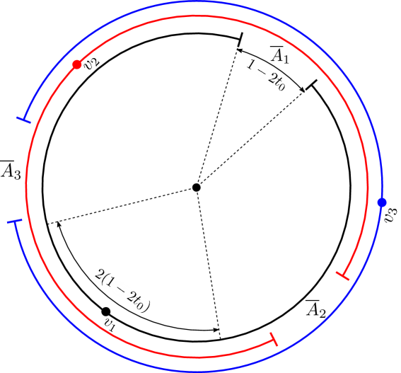
Figure 1: Illustration for the proof of Theorem 4.3. The colored circles represent the sets $A_{i}$ for $v_{1},v_{2},v_{3}$. The probability that $v_{2}$ is placed in the region indicated by the black circular arc such that $\overline{A}_{1}\cap\overline{A}_{2}=\emptyset$ is at least $1-3(1-2t_{0})$ as indicated by the black arrows.

Theorem 4.5 (Lower Bound).

Let $G=\operatorname{GIRG}(n,\beta,w_{0},d)$ be a standard GIRG with $d=\omega(\log(n))$, let $U_{k}=\{v_{1},\ldots,v_{k}\}$ be a set of $k$ random vertices. Then, for every $\mathcal{A}\subseteq\binom{U_{k}}{2}$,

$$\mathrm{Pr}\left[E(U_{k})\supseteq\mathcal{A}\mid\{\kappa\}^{(k)}\right]\geq\prod_{i=1}^{k}\left(1-\sum_{\{i,j\}\in\mathcal{A}_{i}^{-}}\left(1-\left(\frac{\kappa_{ij}}{n}\right)^{1/d}\right)\right)^{d}$$

where $\mathcal{A}_{i}^{-}=\{\{i,j\}\in\mathcal{A}\mid j\leq i\}$ is the set of edges in $\mathcal{A}$ between vertex $i$ and a previous vertex.

Proof 4.6.

We sample the position of $v_{2},\ldots,v_{k}$ one after another and again only consider the probability $p$ that $U_{k}$ is a clique in one fixed dimension. When the position of $v_{i}$ is sampled, the probability that $v_{i}$ falls into one of $A_{ji}$ for $\{i,j\}\in\mathcal{A}_{i}$ is at least

$$1-\sum_{\{i,j\}\in\mathcal{A}_{i}^{-}}\left(1-\left(\frac{\kappa_{ij}}{n}\right)^{1/d}\right),$$

where equality holds if the first $i-1$ vertices are placed such that all the sets $\overline{A}_{ji}$ for $1\leq j<i$ are disjoint. Accordingly, we have

$$p\geq\prod_{i=1}^{k}\left(1-\sum_{\{i,j\}\in\mathcal{A}_{i}^{-}}\left(1-\left(\frac{\kappa_{ij}}{n}\right)^{1/d}\right)\right).$$

To form a clique, it is sufficient that this event occurs in all dimensions, so the final bound is $p^{d}$.

To see how these bounds behave as $n\rightarrow\infty$, we need the following lemma.

Lemma 4.7.

Let $\Psi,d,\ell$ be non-negative functions of $n$. Assume that $\frac{-\ell\ln(\Psi)}{d}=o(1)$ and $\Psi<1$ for all $n$. Then,

$$\frac{-\ell\ln(\Psi)}{d}-e\left(\frac{-\ell\ln(\Psi)}{d}\right)^{2}\leq 1-\Psi^{\ell/d}\leq\frac{-\ell\ln(\Psi)}{d}.$$

Proof 4.8.

Observe that

$$1-\Psi^{\ell/d}=1-\exp\left(\frac{\ell\ln(\Psi)}{d}\right).$$

For the upper bound, we use the well known fact that, for all $x$, we have $\exp(x)\geq 1+x$, which directly implies our statement. For the lower bound, we use the Taylor series expansion of $\exp$ and bound

$$1-\Psi^{\ell/d}=1-\exp\left(\frac{\ell\ln(\Psi)}{d}\right) =-\sum_{i=1}^{\infty}\frac{1}{i!}\left(\frac{\ell\ln(\Psi)}{d}\right)^{i}$$

$$=\sum_{i=1}^{\infty}\frac{(-1)^{i-1}}{i!}\left(\frac{-\ell\ln(\Psi)}{d}\right)^{i}$$

$$=\frac{-\ell\ln(\Psi)}{d}-\left(\frac{-\ell\ln(\Psi)}{d}\right)^{2}\sum_{i=2}^{\infty}\frac{(-1)^{i}}{i!}\left(\frac{-\ell\ln(\Psi)}{d}\right)^{i-2}$$ (7)

Because $\frac{-\ell\ln(\Psi)}{d}=o(1)$, we get that $\left(\frac{-\ln(\Psi)}{d}\right)^{i-2}\leq 1$ for all $i\geq 2$ and sufficiently large $n$. Assuming that all the terms in the above sum are positive yields

$$1-\Psi^{\ell/d} \geq\frac{-\ell\ln(\Psi)}{d}-\left(\frac{-\ell\ln(\Psi)}{d}\right)^{2}\sum_{i=0}^{\infty}\frac{1}{i!}$$

$$=\frac{-\ell\ln(\Psi)}{d}-e\left(\frac{-\ell\ln(\Psi)}{d}\right)^{2}$$

as desired.

Lemma 4.9.

Let

$$P\coloneqq\left(1-\left(\frac{\kappa_{0}}{n}\right)^{r/d}\sum_{\{i,j\}\in\mathcal{A}}\left(1-\left(\frac{\kappa_{ij}}{n}\right)^{1/d}\right)\right)^{d}.$$

Then there is a constant $\delta\geq 0$ such that

$$\ln(P)\leq\sum_{\{i,j\}\in\mathcal{A}}\ln\left(\frac{\kappa_{ij}}{n}\right)\left(1-\frac{\delta\ln(n)}{d}\right).$$

Proof 4.10.

We have

$$\ln(P)=d\ln\left(1-\left(\frac{\kappa_{0}}{n}\right)^{r/d}\sum_{\{i,j\}\in\mathcal{A}}\left(1-\left(\frac{\kappa_{ij}}{n}\right)^{1/d}\right)\right).$$

We get from a Taylor series that

$$\ln(x)=\sum_{i=1}^{\infty}(-1)^{i-1}\frac{(x-1)^{i}}{i}=-\sum_{i=1}^{\infty}\frac{(1-x)^{i}}{i}$$

and thus

$$\ln(P) =-d\sum_{i=1}^{\infty}\frac{1}{i}\left(\left(\frac{\kappa_{0}}{n}\right)^{r/d}\sum_{\{i,j\}\in\mathcal{A}}\left(1-\left(\frac{\kappa_{0}}{n}\right)^{1/d}\right)\right)^{i}$$

$$\leq-d\left(\frac{\kappa_{0}}{n}\right)^{r/d}\sum_{\{i,j\}\in\mathcal{A}}\left(1-\left(\frac{\kappa_{ij}}{n}\right)^{1/d}\right).$$

We now apply the lower bound from Lemma 4.7 with $\Psi=\kappa_{ij}/n$. Note that this fulfills the condition $-\ln(\Psi)/d=o(1)$ as $d=\omega(\log(n))$ and $\kappa_{ij}/n=\Omega(1/n)$. We obtain

$$\ln(P) \leq d\left(\frac{\kappa_{0}}{n}\right)^{r/d}\sum_{\{i,j\}\in\mathcal{A}}\left(\frac{\ln\left(\frac{\kappa_{ij}}{n}\right)}{d}+\frac{e\ln^{2}\left(\frac{\kappa_{ij}}{n}\right)}{d^{2}}\right)$$

$$=\left(\frac{\kappa_{0}}{n}\right)^{r/d}\sum_{\{i,j\}\in\mathcal{A}}\ln\left(\frac{\kappa_{ij}}{n}\right)\left(1-\frac{e}{d}\ln\left(\frac{n}{\kappa_{0}}\right)\right).$$

Note that the above term is negative, so we need to lower bound the term $\left(\frac{\kappa_{0}}{n}\right)^{r/d}$ to proceed. We get from Lemma 4.7,

$$\left(\frac{\kappa_{0}}{n}\right)^{r/d}\geq 1-\frac{r}{d}\ln\left(\frac{n}{\kappa_{0}}\right)-\frac{er^{2}}{d^{2}}\ln\left(\frac{n}{\kappa_{0}}\right)^{2}=1-\frac{c\ln(n)}{d}$$

for some constant $c>0$ and sufficiently large $n$. With this,

$$\ln(P) \leq\sum_{\{i,j\}\in\mathcal{A}}\ln\left(\frac{\kappa_{ij}}{n}\right)\left(1-\frac{e}{d}\ln\left(\frac{n}{\kappa_{0}}\right)\right)\left(1-\frac{c\ln(n)}{d}\right)$$

$$\leq\sum_{\{i,j\}\in\mathcal{A}}\ln\left(\frac{\kappa_{ij}}{n}\right)\left(1-\frac{\delta\ln(n)}{d}\right)$$

for some $\delta>0$ and sufficiently large $n$.

Lemma 4.11.

Let

$$Q\coloneqq\prod_{i=1}^{k}\left(1-\sum_{\{i,j\}\in\mathcal{A}_{i}^{-}}\left(1-\left(\frac{\kappa_{ij}}{n}\right)^{1/d}\right)\right)^{d}.$$

Then there is a constant $\delta$ such that

$$\ln(Q)\geq\sum_{\{i,j\}\in\mathcal{A}}\ln\left(\frac{\kappa_{ij}}{n}\right)\left(1+\frac{\delta\ln(n)}{d}\right).$$

Proof 4.12.

By the upper bound from Lemma 4.7 and the Taylor series of $\ln$, we obtain

$$\ln(Q) \coloneqq d\sum_{i=1}^{k}\ln\left(1-\sum_{\{i,j\}\in\mathcal{A}_{i}^{-}}\left(1-\left(\frac{\kappa_{ij}}{n}\right)^{1/d}\right)\right)$$

$$\geq d\sum_{i=1}^{k}\ln\left(1-\sum_{\{i,j\}\in\mathcal{A}_{i}^{-}}\left(\frac{\ln\left(\frac{n}{\kappa_{ij}}\right)}{d}\right)\right)$$

$$=-d\sum_{i=1}^{k}\sum_{\ell=1}^{\infty}\frac{1}{\ell}\left(\sum_{\{i,j\}\in\mathcal{A}_{i}^{-}}\left(\frac{\ln\left(\frac{n}{\kappa_{ij}}\right)}{d}\right)\right)^{\ell}$$

$$=-d\sum_{i=1}^{k}\sum_{\{i,j\}\in\mathcal{A}_{i}^{-}}\left(\frac{\ln\left(\frac{n}{\kappa_{ij}}\right)}{d}\right)\sum_{\ell=1}^{\infty}\frac{1}{\ell}\left(\sum_{\{i,j\}\in\mathcal{A}_{i}^{-}}\left(\frac{\ln\left(\frac{n}{\kappa_{ij}}\right)}{d}\right)\right)^{\ell-1}$$

$$=\sum_{\{i,j\}\in\mathcal{A}}\ln\left(\frac{\kappa_{ij}}{n}\right)\sum_{\ell=1}^{\infty}\frac{1}{\ell}\left(\sum_{\{i,j\}\in\mathcal{A}_{i}^{-}}\left(\frac{\ln\left(\frac{n}{\kappa_{ij}}\right)}{d}\right)\right)^{\ell-1}$$

$$\geq\sum_{\{i,j\}\in\mathcal{A}}\ln\left(\frac{\kappa_{ij}}{n}\right)\sum_{\ell=1}^{\infty}\frac{1}{\ell}\left(\frac{k\ln\left(\frac{n}{\kappa_{0}}\right)}{d}\right)^{\ell-1}.$$

Now, we have

$$\sum_{\ell=1}^{\infty}\frac{1}{\ell}\left(\frac{k\ln\left(\frac{n}{\kappa_{0}}\right)}{d}\right)^{\ell-1}\leq 1+\frac{k\ln\left(\frac{n}{\kappa_{0}}\right)}{d}\sum_{\ell=0}^{\infty}\left(\frac{k\ln\left(\frac{n}{\kappa_{0}}\right)}{d}\right)^{\ell}\leq 1+\frac{2k\ln\left(\frac{n}{\kappa_{0}}\right)}{d}$$

because $\frac{k\ln\left(\frac{n}{\kappa_{0}}\right)}{d}=o(1)$ and so the above geometric sum converges to $1+o(1)$.

Proof 4.13 (Proof of Theorem 1.2).

Combining Theorem 4.3, Theorem 4.5 Lemma 4.9 and Theorem 4.5, we get that there are constants $\delta,\delta^{\prime}>0$ such that

$$\prod_{\{i,j\}\in\mathcal{A}}\left(\frac{\kappa_{ij}}{n}\right)^{1+\frac{\delta\ln(n)}{d}}\leq\mathrm{Pr}\left[E(U_{k})\supseteq\mathcal{A}\mid\{\kappa\}^{(k)}\right]\leq\prod_{\{i,j\}\in\mathcal{A}}\left(\frac{\kappa_{ij}}{n}\right)^{1-\frac{\delta^{\prime}\ln(n)}{d}}.$$

If $d=\omega(\log(n))$, $\frac{\delta\ln(n)}{d}=o(1)$ and the first part of the statement is shown. For the second part observe that

$$\prod_{\{i,j\}\in\mathcal{A}}\left(\frac{\kappa_{ij}}{n}\right)^{1+\frac{\delta\ln(n)}{d}}\geq\left(\frac{n}{\kappa_{0}}\right)^{\binom{k-1}{2}\frac{\delta\ln(n)}{d}}\prod_{\{i,j\}\in\mathcal{A}}\left(\frac{\kappa_{ij}}{n}\right).$$

Similarly,

$$\prod_{\{i,j\}\in\mathcal{A}}\left(\frac{\kappa_{ij}}{n}\right)^{1-\frac{\delta^{\prime}\ln(n)}{d}}\leq\left(\frac{n}{\kappa_{0}}\right)^{\binom{k-1}{2}\frac{\delta^{\prime}\ln(n)}{d}}\prod_{\{i,j\}\in\mathcal{A}}\left(\frac{\kappa_{ij}}{n}\right).$$

If $d=\omega(\log^{2}(n))$, we get that

$$\left(\frac{n}{\kappa_{0}}\right)^{\binom{k-1}{2}\frac{\delta\ln(n)}{d}}=(1+o(1))n^{1/\omega(\log(n))}=(1+o(1))\exp\left(\frac{\log(n)}{\omega(\log(n))}\right)=1+o(1)$$

as we assume $k$ to be constant.

4.1.1 Bounds for Triangles

We proceed by deriving a lower bound for the probability that three vertices form a triangle.

Lemma 4.14.

Let $G=\operatorname{GIRG}(n,\beta,w_{0},d)$ be a standard GIRG and let $v_{1},v_{2},v_{3}$ be three random vertices. Then,

$$\mathrm{Pr}\left[v_{2}\sim v_{3}\mid v_{1}\sim v_{2},v_{3}\right]\geq\left(3-3\left(\frac{\kappa_{0}}{n}\right)^{-1/d}+\left(\frac{\kappa_{0}}{n}\right)^{-2/d}\right)^{d}.$$

Proof 4.15.

We consider one fixed dimension and give an upper bound on the probability that $v_{2}\nsim v_{3}$ conditioned on $v_{1}\sim v_{2},v_{3}$. In the following, we abbreviate $p\coloneqq\frac{\kappa_{0}}{n}$. Note that we may assume that all three vertices are of weight $w_{0}$ as it is easy to verify that larger weights only increase the probability of forming a triangle. Conditioned on the event $v_{1}\sim v_{2},v_{3}$, the vertices $v_{2},v_{3}$ are uniformly distributed within a circular arc of length $p^{1/d}$ around $v_{1}$. In order for $v_{2}\nsim v_{3}$ to occur, $v_{3}$ needs to be placed within a circular arc of length $1-p^{1/d}$ opposite to $v_{2}$. Hence, the probability that $v_{2}\nsim v_{3}$ conditioned on the event that $v_{2}$ is placed at distance $x$ of $v_{1}$ is

$$\mathrm{Pr}\left[v_{2}\nsim v_{3}\mid|x_{v_{1}}-x_{v_{2}}|_{C}=x\right]=\begin{cases}x/p^{1/d}&\text{if }x\leq 1-p^{1/d}\\ (1-p^{1/d})/p^{1/d}&\text{otherwise}\end{cases}$$

where $|\cdot|_{C}$ denotes the distance on the circle. Since $v_{2}$ is distributed uniformly within distance $\frac{1}{2}p^{1/d}$ around $v_{1}$, we obtain

$$\mathrm{Pr}\left[v_{2}\nsim v_{3}\mid v_{1}\sim v_{2},v_{3}\right] \leq\frac{1}{\frac{1}{2}p^{1/d}}\int_{0}^{\frac{1}{2}p^{1/d}}\mathrm{Pr}\left[v_{2}\nsim v_{3}\mid|x_{v_{1}}-x_{v_{2}}|_{C}=x\right]\mathrm{d}x$$

$$=\frac{1}{\frac{1}{2}p^{1/d}}\left(\int_{0}^{1-p^{1/d}}\frac{x}{p^{1/d}}\mathrm{d}x+\int_{1-p^{1/d}}^{\frac{1}{2}p^{1/d}}\frac{1-p^{1/d}}{p^{1/d}}\mathrm{d}x\right).$$

Solving the integrals then yields

$$\mathrm{Pr}\left[v_{2}\nsim v_{3}\mid v_{1}\sim v_{2},v_{3}\right]\leq 3p^{-1/d}-2-p^{-2/d}$$

implying the desired bound.

We use this finding to show in the following lemma that, although cliques of size at least $4$ already behave like in the IRG model if $d=\omega(\log(n))$, the number of triangles in the geometric case is still larger than that in the non-geometric case.

Lemma 4.16.

Let $G=\operatorname{GIRG}(n,\beta,w_{0},d)$ be a standard GIRG with $d=\omega(\log(n))$ and let $v_{1},v_{2},v_{3}$ be three random vertices. Then,

$$\mathrm{Pr}\left[v_{2}\sim v_{3}\mid v_{1}\sim v_{2},v_{3}\right]\geq(1+o(1))\left(\frac{\kappa_{0}}{n}\right)^{1-\frac{3\ln(n)^{2}}{4d^{2}}\pm\mathcal{O}\left(\frac{\ln(n)^{3}}{d^{3}}\right)}.$$

Proof 4.17.

By Lemma 4.14, we have $\mathrm{Pr}\left[v_{2}\sim v_{3}\mid v_{1}\sim v_{2},v_{3}\right]=q^{d}$ with

$$q\coloneqq 3\left(1-\left(\frac{\kappa_{0}}{n}\right)^{-1/d}\right)+\left(\frac{\kappa_{0}}{n}\right)^{-2/d}.$$

In the following, we once again abbreviate $p=\frac{\kappa_{0}}{n}$ and start by decomposing $q$ into a sum.

$$q =3\left(1-p^{-1/d}\right)+p^{-2/d}$$

$$=3\left(1-\exp\left(\frac{-\ln(p)}{d}\right)\right)+\exp\left(\frac{-2\ln(p)}{d}\right)$$

$$=-3\sum_{i=1}^{\infty}\frac{1}{i!}\left(\frac{-\ln(p)}{d}\right)^{i}+\sum_{i=0}^{\infty}\frac{1}{i!}\left(\frac{-2\ln(p)}{d}\right)^{i}$$

$$=1+\sum_{i=1}^{\infty}\frac{1}{i!}\left(\left(\frac{-2\ln(p)}{d}\right)^{i}-3\left(\left(\frac{-\ln(p)}{d}\right)^{i}\right)\right)$$

$$=1+\sum_{i=1}^{\infty}\frac{1}{i!}\left(\frac{-\ln(p)}{d}\right)^{i}(2^{i}-3).$$

We now proceed by bounding $d\ln(q)$ and apply the Taylor series of $\ln$ to get

$$d\ln(q)=-d\sum_{i=1}\frac{(1-q)^{i}}{i}=\sum_{i=1}(-1)^{i+1}d\frac{(q-1)^{i}}{i}.$$ (8)

By abbreviating $x\coloneqq\ln(p)/d$ and our above sum, we get

$$q-1=\sum_{i=1}^{\infty}\frac{1}{i!}\left(\frac{-\ln(p)}{d}\right)^{i}(2^{i}-3) =x+\frac{1}{2}x^{2}-\frac{5}{6}x^{3}+\ldots$$

$$=x\underbrace{\left(1+\frac{1}{2}x-\frac{5}{6}x^{2}+R\right)}_{Z},$$ (9)

where $|R|=\mathcal{O}(|x|^{3})$ because $|x|=o(1).$. Inserting this into the first terms of the sum in Equation 8 yields

$$d\ln(q) =dxZ-d\frac{1}{2}x^{2}Z^{2}+d\frac{1}{3}x^{3}Z^{3}+\ldots$$

$$=dx\left(Z-\frac{1}{2}xZ^{2}+\frac{1}{3}x^{2}Z^{3}+\sum_{i=4}(-1)^{i+1}x^{i-1}Z^{i}\right).$$

Using the definition of $Z$ in 4.17, we may carefully compute the leading terms of the above sum to obtain

$$d\ln(q)=dx\left(1-\frac{3}{4}x^{2}+R^{\prime}\right),$$

with $|R^{\prime}|=\mathcal{O}(|x|^{3})$. Recalling that $x=\ln(p)/d$ gives

$$d\ln(q)=\ln(p)\left(1-\frac{3}{4}\left(\frac{\ln(p)}{d}\right)^{2}\pm\mathcal{O}\left(\left|\frac{\ln(p)}{d}\right|^{3}\right)\right).$$

As $p=\kappa_{0}/n$, this shows

$$q^{d}=\left(\frac{\kappa_{0}}{n}\right)^{1-\frac{3\ln(n/\kappa_{0})^{2}}{4d^{2}}\pm\mathcal{O}\left(\frac{\ln(n)^{3}}{d^{3}}\right)}=(1+o(1))\left(\frac{\kappa_{0}}{n}\right)^{1-\frac{3\ln(n)^{2}}{4d^{2}}\pm\mathcal{O}\left(\frac{\ln(n)^{3}}{d^{3}}\right)}.$$

Here, the factor of $1+o(1)$ derives from the fact that $\frac{\ln(n/\kappa_{0})^{2}}{d^{2}}=\frac{\ln(n)^{2}-2\ln(n)\ln(\kappa_{0})+\ln(\kappa_{0})^{2}}{d^{2}}=\frac{\ln(n)^{2}}{d^{2}}-\frac{1}{\omega(\log(n))}$

The above bound implies that the probability that a triangle forms among vertices of constant weight is still significantly larger than in the non-geometric models as long as $d=o\left(\log^{3/2}(n)\right)$. We summarize this behavior in the following theorem.

Theorem 4.18.

Let $G=\operatorname{GIRG}(n,\beta,w_{0},d)$ be a standard GIRG with $\beta>3$ and $d=\omega(\log(n))$. Then, there is a constant $\delta\geq 0$ such that the expected number of triangles fulfills

$$\mathbb{E}\left[K_{3}\right]=\Omega\left(\exp\left(\frac{\ln^{3}(n)}{d^{2}}\right)\right).$$

For $\beta=\infty$ (that is the case of constant weights) we have

$$\mathbb{E}\left[K_{3}\right]=\Theta\left(\exp\left(\frac{\ln^{3}(n)}{d^{2}}\right)\right).$$

Proof 4.19.

We note that, by Lemma 4.16

$$\mathbb{P}_{3}\geq(1+o(1))\left(\frac{\kappa_{0}}{n}\right)^{2}\left(\frac{\kappa_{0}}{n}\right)^{1-\frac{3\ln(n)^{2}}{4d^{2}}\pm\mathcal{O}\left(\frac{\ln(n)^{3}}{d^{3}}\right)}$$

and thus

$$\mathbb{E}\left[K_{3}\right]=\binom{n}{3}\mathbb{P}_{3}\geq(1+o(1))\kappa_{0}^{3}n^{\Omega\left(\frac{\ln^{2}(n)}{d^{2}}\right)}=\Omega\left(\exp\left(\frac{\ln^{3}(n)}{d^{2}}\right)\right)$$

and the first part of the statement is shown. For the second part, we note that in the case of constant weights, the bound from Lemma 4.14 is the exact (conditional) probability that a triangle is formed and the transformations from Lemma 4.16 still apply for obtaining an upper bound.

4.2 Bounds on $\mathbb{E}\left[K_{k}\right]$ and $\omega(G)$

We use the findings from section Section 4.1 to prove the third column of Table 3 and Table 1, respectively. We treat the cases $2<\beta<3$, $\beta=3$, and $\beta>3$ separately.

For $\beta\in(2,3)$, we show that if $d=\omega(\log(n))$, then the expected number of cliques is $n^{\frac{k}{2}(3-\beta)}\Theta(k)^{-k}$ for all $k\geq 3$ just like in the IRG model. This is despite the fact that the probability that a clique forms among vertices of constant weight is still significantly higher than in the IRG model if $\log(n)\ll d\ll\log^{3/2}(n)$. The reason for this is that the probability of forming a clique among vertices of weight close to $\sqrt{n}$ behaves like that of the IRG model if $d=\omega(\log(n))$ and because cliques forming among these high-weight vertices dominate all the others.

Theorem 4.20.

Let $G=\operatorname{GIRG}(n,\beta,w_{0},d)$ be a standard GIRG with $\beta<3$ and $d=\omega(\log(n))$. Then, $\mathbb{E}[K_{k}]=n^{\frac{k}{2}(3-\beta)}\Theta(k)^{-k}$ for $k\geq 3$ and $\omega(G)=\Theta(n^{(3-\beta)/2})$ a.a.s.

Proof 4.21.

Observe that Corollary 3.5 and Corollary 3.9 imply our desired bounds if $k>\frac{2}{3-\beta}$. We may thus assume that $k\leq\frac{2}{3-\beta}$, which is at most a constant. To upper bound $q_{k}$, recall that $U_{k}=\{v_{1},\ldots,v_{k}\}$ is a set of $k$ vertices chosen independently and uniformly at random and have weights $w_{1},\ldots,w_{k}$, respectively. In the following, we assume $w_{1}\leq w_{2}\leq\ldots\leq w_{k}$ and we use a similar technique like Daly et al. [14] who bound

$$q_{k} \leq\mathrm{Pr}\left[(U_{k}\text{ is clique })\cap(w_{k}\leq\sqrt{n/\lambda})\right]+\sum_{m=1}^{k-1}\binom{k}{m}P_{k,m}$$

$$\hskip 28.45274pt+\mathrm{Pr}\left[(U_{k}\text{ is clique })\cap(w_{1}\geq\sqrt{n/\lambda})\right],$$

where

$$P_{k,m}\coloneqq\mathrm{Pr}\left[(U_{k}\text{ is clique })\cap(w_{m}\leq\sqrt{n/\lambda})\cap(w_{m+1}\geq\sqrt{n/\lambda})\right].$$

That is, we bound the probability that a clique is formed by summing over the probability that a clique is formed with the additional condition that $m$ vertices are of weight below $\sqrt{n/\lambda}$ and $k-m$ vertices are of weight at least $\sqrt{n/\lambda}$ for all $m$.

We start with the first extreme case and observe that

$$\mathrm{Pr}\left[(U_{k}\text{ is clique })\cap(w_{k}\leq\sqrt{n/\lambda})\right]\leq\int_{w_{0}}^{\sqrt{n/\lambda}}\cdots\int_{w_{0}}^{\sqrt{n/\lambda}}\mathbb{P}_{k\mid w}\rho(w_{1})\cdots\rho(w_{k})\mathrm{d}w_{1}\ldots\mathrm{d}w_{k}.$$

By Theorem 1.2, we get that there is a function $\varepsilon(n)=o(1)$ such that

$$\begin{split}&\mathrm{Pr}\left[(U_{k}\text{ is clique })\cap(w_{k}\leq\sqrt{n/\lambda})\right]\leq\\ &\hskip 28.45274pt\Theta(1)\int_{w_{0}}^{\sqrt{n/\lambda}}\cdots\int_{w_{0}}^{\sqrt{n/\lambda}}\prod_{1\leq i<j\leq k}\left(\frac{\kappa_{ij}}{n}\right)^{1-\varepsilon}w_{1}^{-\beta}\cdots w_{k}^{-\beta}\mathrm{d}w_{1}\ldots\mathrm{d}w_{k}\end{split}$$

$$=\Theta(1)n^{-\binom{k}{2}(1-\varepsilon)}\left(\int_{w_{0}}^{\sqrt{n/\lambda}}w^{(k-1)(1-\varepsilon)-\beta}\mathrm{d}w\right)^{k}$$

$$=\Theta(1)n^{-\binom{k}{2}(1-\varepsilon)}n^{\frac{1}{2}k(k-1)(1-\varepsilon)+\frac{k}{2}(1-\beta)}$$

$$=\Theta(1)n^{\frac{k}{2}(1-\beta)}$$

as $\binom{k}{2}=\frac{1}{2}k(k-1)$. note that the above bounds only hold for sufficiently large $n$ as $\varepsilon=o(1)$. For the other extreme case, Corollary 3.5 yields that

$$\mathrm{Pr}\left[(U_{k}\text{ is clique })\cap(w_{1}\geq\sqrt{n/\lambda})\right]\leq\mathrm{Pr}\left[w_{1}\geq\sqrt{n/\lambda}\right]=\Theta(1)n^{\frac{k}{2}(1-\beta)}.$$

We proceed by bounding $P_{k,m}$. If $m\geq 3$, we bound the probability that a clique is formed by considering the necessary event that the first $m$ vertices form a clique and the remaining $k-m$ vertices do so as well. As these two events are disjoint, we may reuse the above bounds and obtain

$$P_{k,m} \leq\mathrm{Pr}\left[U_{m}\text{ is clique }\cap w_{m}\leq\sqrt{n/\lambda}\right]\mathrm{Pr}\left[U_{k-m}\text{ is clique }\cap w_{1}\geq\sqrt{n/\lambda}\right]$$

$$=\Theta(1)n^{\frac{m}{2}(1-\beta)}n^{\frac{k-m}{2}(1-\beta)}$$

$$=\Theta(1)n^{\frac{k}{2}(1-\beta)}$$

as desired. It thus remains the case $m=\{1,2\}$. For $m=1$, we bound the probability $P_{1}$ that $v_{1}$ connects to $v_{2}$ and $v_{3}$ where $w_{1}\leq\sqrt{n/\lambda}$ and $w_{2},w_{3}\geq\sqrt{n/\lambda}$. We get

$$\begin{split}&P_{1}\leq\\ &\hskip 28.45274pt\Theta(1)\int_{w_{0}}^{\sqrt{n/\lambda}}\int_{\sqrt{n/\lambda}}^{\infty}\int_{\sqrt{n/\lambda}}^{\infty}\left(\frac{w_{1}^{2}w_{2}w_{3}}{n}\right)^{2(1-\varepsilon)}w_{1}^{-\beta}w_{2}^{-\beta}w_{3}^{-\beta}\mathrm{d}w_{1}\mathrm{d}w_{2}\mathrm{d}w_{3}\end{split}$$

$$=\Theta(1)n^{-2(1-\varepsilon)}\int_{w_{0}}^{\sqrt{n/\lambda}}w^{2(1-\varepsilon)-\beta}\mathrm{d}w\left(\int_{\sqrt{n/\lambda}}^{\infty}w^{1-\varepsilon-\beta}\mathrm{d}w\right)^{2}$$

$$=\Theta(1)n^{-2(1-\varepsilon)+(1-\varepsilon)+\frac{1}{2}(1-\beta)+(1-\varepsilon)+(1-\beta)}$$

$$=\Theta(1)n^{\frac{3}{2}(1-\beta)}$$

as desired. For the case $m=2$, we need to be a little more creative and bound the probability $P_{2}$ that $v_{1},v_{2},v_{3}$ form a triangle ($w_{1},w_{2}\leq\sqrt{n/\lambda}$, $w_{3}\geq\sqrt{n/\lambda}$) as follows

$$\begin{split}&P_{2}\leq\Theta(1)\underbrace{\int_{w_{0}}^{\sqrt{n/\lambda}}\int_{w_{0}}^{w_{1}}\int_{\sqrt{n/\lambda}}^{n/w_{1}}\prod_{1\leq i<j\leq 3}\left(\frac{w_{i}w_{j}}{n}\right)^{1-\varepsilon}(w_{1}w_{2}w_{3})^{-\beta}\mathrm{d}w_{3}\mathrm{d}w_{2}\mathrm{d}w_{1}}_{I_{1}}\\ &\hskip 5.69046pt+\Theta(1)\underbrace{\int_{w_{0}}^{\sqrt{n/\lambda}}\int_{w_{0}}^{w_{1}}\int_{n/w_{1}}^{\infty}\left(\frac{w_{1}^{2}w_{2}w_{3}}{n}\right)^{2(1-\varepsilon)}(w_{3}w_{2}w_{1})^{-\beta}\mathrm{d}w_{3}\mathrm{d}w_{2}\mathrm{d}w_{1}}_{I_{2}}.\end{split}$$

Note that this is a valid bound since the vertices $v_{1},v_{2}$ are interchangeable and thus $P_{2}$ is at most twice as large as the two integrals above, which is captured by the $\Theta(1)$ terms. Calculations now show that

$$I_{1}=\Theta(1)n^{\frac{3}{2}(1-\beta)}\text{ and }I_{2}=\Theta(1)n^{\frac{3}{2}(1-\beta)}$$

as desired. This implies that $\mathbb{E}[K_{k}]=n^{\frac{k}{2}(3-\beta)}\Theta(k)^{-k}$.

We note that the phase transition at $k=\frac{2}{3-\beta}$ is not present anymore. We continue with the case where $\beta=3$.

Theorem 4.22.

Let $G=\operatorname{GIRG}(n,\beta,w_{0},d)$ be a standard GIRG with $\beta=3$ and $d=\omega(\log(n))$. Then, $\omega(G)=\mathcal{O}(1)$.

Proof 4.23.

If $\beta=3$ the situation is similar. We show that the number of cliques of size $k=4$ is such that for every $\varepsilon>0$ there is a constant $c>0$ such that

$$\mathrm{Pr}\left[K_{4}\geq c\right]\leq\varepsilon.$$

That is, the probability that $K_{4}\geq c$ can be made arbitrarily small by choosing $c$ large enough. This fact is sufficient to show that the clique number is $\Theta(1)$.

We start by observing that $\beta=3$ implies that the maximum weight $w_{max}$ is a.a.s. in the order $\sqrt{n}$. More precisely, denoting by $X_{w}$ the number of vertices with weight at least $w$, we get by Markov’s inequality that for every $w$,

$$\mathrm{Pr}\left[w_{max}\geq w\right]=\mathrm{Pr}\left[X_{w}\geq 1\right]\leq\mathbb{E}\left[X_{w}\right]=\Theta(1)nw^{1-\beta}=\Theta(1)nw^{-2}.$$ (10)

Thus, for every $c\geq 0$, we have

$$\mathrm{Pr}\left[w_{max}\geq c\sqrt{n}\right]=\mathcal{O}(1)c^{-2}.$$ (11)

With this and Markov’s inequality, we may bound for every $t,c\geq 0$

$$\mathrm{Pr}\left[K_{4}\geq t\right] \leq\mathrm{Pr}\left[K_{4}\geq t\mid w_{max}\leq c\sqrt{n}\right]+\mathrm{Pr}\left[w_{max}\geq c\sqrt{n}\right]$$

$$\leq\frac{\mathbb{E}\left[K_{4}\mid w_{max}\leq c\sqrt{n}\right]}{t}+\mathrm{Pr}\left[w_{max}\geq c\sqrt{n}\right].$$ (12)

To bound $\mathbb{E}\left[K_{4}\mid w_{max}\leq c\sqrt{n}\right]$, we note that a random weight $w_{i}$ fulfills

$$\mathrm{Pr}\left[w_{i}\leq x\mid w_{max}\leq c\sqrt{n}\right] =\frac{\mathrm{Pr}\left[\bigcap_{j}w_{j}\leq c\sqrt{n}\cap w_{i}\leq x\right]}{\mathrm{Pr}\left[\bigcap_{j}w_{j}\leq c\sqrt{n}\right]}$$

$$=\frac{\mathrm{Pr}\left[w_{i}\leq x\right]}{\mathrm{Pr}\left[w_{i}\leq c\sqrt{n}\right]}$$

and since $\mathrm{Pr}\left[w_{i}\leq c\sqrt{n}\right]=1-o(1)$, we get that the density of $w_{i}$ is $\rho_{w_{i}}(x)=c^{\prime}x^{-\beta}$ for some $c^{\prime}\geq 0$ independent of $x$. Using that, we use Theorem 1.2 to bound

$$\begin{split}&\mathrm{Pr}\left[U_{k}\text{ is clique }\mid w_{k}\leq c\sqrt{n}\right]\leq\\ &\hskip 28.45274pt\Theta(1)\int_{w_{0}}^{c\sqrt{n}}\cdots\int_{w_{0}}^{c\sqrt{n}}\prod_{1\leq i<j\leq k}\left(\frac{\kappa_{ij}}{n}\right)^{1-\varepsilon}w_{1}^{-\beta}\cdots w_{k}^{-\beta}\mathrm{d}w_{1}\ldots\mathrm{d}w_{k}\end{split}$$

$$=\Theta(1)n^{-\binom{k}{2}(1-\varepsilon)}\left(\int_{w_{0}}^{c\sqrt{n}}w^{(k-1)(1-\varepsilon)-\beta}\mathrm{d}w\right)^{k}$$

for some function $\varepsilon(n)=o(1)$. Because $k\geq 4$ and $\beta=3$, we observe that the exponent $(k-1)(1-\varepsilon)-\beta$ is greater than $-1$ for sufficiently large $n$, and hence, the above integral evaluates to

$$\mathrm{Pr}\left[U_{k}\text{ is clique }\mid w_{k}\leq c\sqrt{n}\right]=c^{k((k-1)(1-\varepsilon)+1-\beta)}\Theta(1)n^{\frac{k}{2}(1-\beta)}.$$

For $k=4$, we obtain

$$\mathrm{Pr}\left[U_{k}\text{ is clique }\mid w_{k}\leq c\sqrt{n}\right]\leq\Theta(1)c^{4}n^{-4}$$

and accordingly

$$\mathbb{E}\left[K_{4}\mid w_{max}\leq c\sqrt{n}\right]=\binom{n}{4}\mathrm{Pr}\left[U_{k}\text{ is clique }\mid w_{k}\leq c\sqrt{n}\right]\leq\Theta(1)c^{4}.$$

By (4.23) and (11), this implies

$$\mathrm{Pr}\left[K_{4}\geq t\right]=\Theta(1)c^{4}t^{-1}+\mathcal{O}(1)c^{-2}.$$

Setting $c=t^{1/5}$ yields $\mathrm{Pr}\left[K_{4}\geq t\right]=\mathcal{O}(1)(t^{-1/5}+t^{-2/5})$ and shows that the probability that $K_{4}\geq t$ can be made arbitrarily small by increasing $t$. To bound the clique number, we note that the existence of a clique of size $k$ implies the existence of $\binom{k}{4}$ cliques of size $4$ and so,

$$\mathrm{Pr}\left[\omega(G)\geq k\right]\leq\mathrm{Pr}\left[K_{4}\geq\binom{k}{4}\right],$$

which can be made arbitrarily small by choosing $k$ large enough. Hence the probability that the clique number grows as any superconstant function $f(n)=\omega(1)$ is in $o(1)$, which shows that the clique number is in $\mathcal{O}(1)$ a.a.s.

Finally, we deal with the case where $\beta>3$, where we show that, in this case, there are no cliques of size $4$ or larger a.a.s.

Theorem 4.24.

Let $G=\operatorname{GIRG}(n,\beta,w_{0},d)$ be a standard GIRG with $\beta>3$ and $d=\omega(\log(n))$. Then, $\mathbb{E}[K_{k}]=o(1)$ for $k\geq 4$ and, thus, $\omega(G)\leq 3$ a.a.s.

Proof 4.25.

We use a similar strategy as in the above paragraph. In analogy to Equation 10, we now have

$$\mathrm{Pr}\left[w_{max}\geq n^{\alpha}\right]\leq\Theta(1)n^{1-(1-\beta)\alpha},$$

which is $o(1)$ if $\alpha>\frac{1}{\beta-1}$. For some $\alpha$ in the range $1/2>\alpha>\frac{1}{\beta-1}$, we get

$$\begin{split}&\mathrm{Pr}\left[U_{k}\text{ is clique }\mid w_{k}\leq n^{\alpha}\right]\leq\\ &\hskip 28.45274pt\Theta(1)\int_{w_{0}}^{n^{\alpha}}\cdots\int_{w_{0}}^{n^{\alpha}}\prod_{1\leq i<j\leq k}\left(\frac{\kappa_{ij}}{n}\right)^{1-\varepsilon}w_{1}^{-\beta}\cdots w_{k}^{-\beta}\mathrm{d}w_{1}\ldots\mathrm{d}w_{k}\end{split}$$

$$=\Theta(1)n^{-\binom{k}{2}(1-\varepsilon)}\left(\int_{w_{0}}^{n^{\alpha}}w^{(k-1)(1-\varepsilon)-\beta}\mathrm{d}w\right)^{k}$$

$$=\Theta(1)n^{\left(\alpha-\frac{1}{2}\right)k(k-1)(1-\varepsilon)+\alpha k(1-\beta)}=o\left(n^{\alpha k(1-\beta)}\right).$$

Accordingly,

$$\mathbb{E}\left[K_{4}\mid w_{max}\leq c\sqrt{n}\right]=\binom{n}{4}\mathrm{Pr}\left[U_{k}\text{ is clique }\mid w_{k}\leq c\sqrt{n}\right]=\Theta(1)n^{4+4\alpha(1-\beta)}=o(1).$$

as $\alpha(1-\beta)<-1$. By Markov’s inequality this implies

$$\mathrm{Pr}\left[K_{4}\geq 1\right]\leq\mathbb{E}\left[K_{4}\mid w_{max}\leq n^{\alpha}\right]+\mathrm{Pr}\left[w_{max}\geq n^{\alpha}\right]=o(1)$$

as desired.

5 Asymptotic Equivalence with IRGs

We continue by investigating the infinite-dimensional limit of our model, i.e., the case where $n$ is fixed and $d$ goes to infinity. We prove that in this situation, the GIRG model becomes in a strong sense equivalent to the non-geometric IRG model. That is, we prove that the total variation distance of the distribution over all possible graphs with $n$ vertices goes to $0$ as $d\rightarrow\infty$. We prove the following

See 1.1

We split the proof of this theorem by considering the case of an $L_{p}$-norm for $1\leq p<\infty$ and the case of $L_{\infty}$-norm separately. Our investigations in Section 1.4 further show why RGGs on the torus become equivalent to non-geometric models as $d$ tends to infinity and why this is not the case if we use the hypercube instead as previously observed in [18, 13].

5.1 Equivalence for $L_{p}$-norms with $1\leq p<\infty$

Our argument builds upon a multivariate central-limit-theorem similar to the one used by Devroye et al. who establish a similar statement for SRGGs [17] .

Before starting the proof, we introduce some necessary auxiliary statements. Our argumentation builds upon the following Berry-Esseen theorem introduced in [36].

Theorem 5.1 (Theorem 1.1 in [36]).

Let $Z_{1},\ldots,Z_{d}$ be independent zero-mean random variables taking values in $\mathbb{R}^{m}$. Let further $Z\coloneqq\sum_{i=1}^{d}Z_{i}$ and assume that the covariance matrix of $Z$ is the identity matrix. Let $X\in\mathbb{R}^{m}$ be a random variable following the standard $m$-variate normal distribution $\mathcal{N}(0,I)$. Then for any convex set $A\subseteq\mathbb{R}^{m}$, we have

$$\left|\mathrm{Pr}\left[Z\in A\right]-\mathrm{Pr}\left[X\in A\right]\right|\leq(42d^{1/4}+16)\sum_{i=1}^{d}\mathbb{E}\left[\left\|Z_{i}\right\|^{3}\right]$$

where $\left\|Z_{i}\right\|$ is the $L_{2}$-norm of $Z_{i}$.

This illustrates that for $d\rightarrow\infty$, the (random) distance between two vertices behaves like a Gaussian random variable. Throughout this section, we use the following notation. For any $u,v\in V$, we define $\Delta_{(u,v)}\in\mathbb{R}^{d}$ as the component-wise distance of $u$ and $v$, i.e., $\Delta_{(u,v),i}\coloneqq\left|\mathbf{x}_{ui}-\mathbf{x}_{vi}\right|_{C}=\min\{\left|\mathbf{x}_{ui}-\mathbf{x}_{vi}\right|,1-\left|\mathbf{x}_{ui}-\mathbf{x}_{vi}\right|\}$. We may express

$$\mathrm{Pr}\left[u\sim v\right]=\mathrm{Pr}\left[\left\|\Delta_{(u,v)}\right\|_{p}\leq t_{uv}\right]=\mathrm{Pr}\left[\sum_{i=1}^{d}\Delta_{(u,v),i}^{p}\leq t_{uv}^{p}\right]$$

and we further note that $\Delta_{(u,v),i}$ and $\Delta_{(u,v),j}$ are i.i.d. random variables. Define

$$\mu\coloneqq\mathbb{E}\left[\Delta_{(u,v),i}^{p}\right]\hskip 14.22636pt\text{and}\hskip 14.22636pt\sigma^{2}\coloneqq\text{Var}\left[\Delta_{(u,v),i}^{p}\right].$$

and let the random variable $Z_{(u,v),i}$ be defined as

$$Z_{(u,v),i}\coloneqq\frac{\Delta_{(u,v),i}^{p}-\mu}{\sqrt{d}\sigma}.$$

Now define $Z_{(u,v)}\coloneqq\sum_{i=1}^{d}Z_{(u,v),i}$ and observe that this allows us to express

$$\mathrm{Pr}\left[u\sim v\right]=\mathrm{Pr}\left[\sum_{i=1}^{d}\Delta_{(u,v),i}^{p}\leq t_{uv}^{p}\right]=\mathrm{Pr}\left[Z_{(u,v)}\leq\frac{t_{uv}^{p}-d\mu}{\sqrt{d}\sigma}\right].$$

Working with $Z_{(u,v)}$ instead of $\Delta_{(u,v)}$ has the advantage that we have $\mathbb{E}\left[Z_{(u,v)}\right]=0$ and

$$\text{Var}\left[Z_{(u,v)}\right]=\sum_{i=1}^{d}\text{Var}\left[Z_{(u,v),i}\right]=\frac{1}{d\sigma^{2}}\sum_{i=1}^{d}\text{Var}\left[\Delta_{(u,v),i}^{p}\right]=1.$$

These properties are useful when applying Theorem 5.1. Now recall that $t_{uv}$ is defined such that the marginal connection probability $\mathrm{Pr}\left[u\sim v\right]$ is equal to $\min\left\{1,\frac{\lambda w_{u}w_{v}}{n}\right\}$, which is required in order to ensure that $\mathbb{E}\left[\deg(v)\right]\propto w_{v}$ for all $v$. We use this to establish the following lemma describing the asymptotic behavior of the threshold $t_{uv}$.

Lemma 5.2.

Let $G=\operatorname{GIRG}(n,\beta,w_{0},d)=(V,E)$ be a standard GIRG with $L_{p}$-norm for $p\in[1,\infty)$. Denote by $\Phi$ the cumulative density function of the standard Gaussian distribution, i.e., $\Phi(x)=\sqrt{2\pi}\int_{-\infty}^{x}e^{-t^{2}/2}dt$. Then for any $u,v\in V$ with $u\neq v$ and $\frac{\lambda w_{u}w_{v}}{n}<1$, we have

$$\lim_{d\rightarrow\infty}\frac{t_{uv}^{p}-d\mu}{\sqrt{d}\sigma}=\Phi^{-1}\left(\frac{\lambda w_{u}w_{v}}{n}\right).$$

Proof 5.3.

Let $u,v$ be fixed. In the remainder of this proof, we abbreviate $Z_{(u,v)}$ with $Z$, and $Z_{(u,v),i}$ with $Z_{i}$. For every $c\in\mathbb{R}$, define the set $A_{c}=\left\{x\in\mathbb{R}\mid x\leq c\right\}$. Let further $X\sim\mathcal{N}(0,1)$ be a standard Gaussian random variable. We get from Theorem 5.1 that

$$\left|\mathrm{Pr}\left[Z\leq c\right]-\mathrm{Pr}\left[X\leq c\right]\right| \leq(42d^{1/4}+16)\sum_{i=1}^{d}\mathbb{E}\left[\left|Z_{i}\right|^{3}\right]$$

$$=\frac{42d^{1/4}+16}{d^{3/2}\sigma^{3}}\sum_{i=1}^{d}\mathbb{E}\left[\left|\Delta_{(u,v),i}^{p}-\mu\right|^{3}\right]$$

$$\leq\frac{42d^{1/4}+16}{d^{1/2}\sigma^{3}}$$ (13)

$$=o_{d}(1)$$ (14)

because $\Delta_{(u,v),i}^{p}-\mu\in[-1,1]$, which shows that $Z$ converges to a standard Gaussian random variable as $d\rightarrow\infty$. In particular, this statement is true for $c=\Phi^{-1}\left(\frac{\lambda w_{u}w_{v}}{n}\right)$. At the same time,

$$\mathrm{Pr}\left[X\leq\Phi^{-1}\left(\frac{\lambda w_{u}w_{v}}{n}\right)\right]=\frac{\lambda w_{u}w_{v}}{n}=\mathrm{Pr}\left[Z\leq\frac{t_{uv}^{p}-d\mu}{\sqrt{d}\sigma}\right],$$

where the second step follows by the definition of $t_{uv}$ and $Z$. Hence, by (5.3),

$$\lim_{d\rightarrow\infty}\left|\mathrm{Pr}\left[Z\leq\Phi^{-1}\left(\frac{\lambda w_{u}w_{v}}{n}\right)\right]-\mathrm{Pr}\left[Z\leq\frac{t_{uv}^{p}-d\mu}{\sqrt{d}\sigma}\right]\right|=0.$$

Since the function $f(c)=\mathrm{Pr}\left[Z\leq c\right]$ converges to the cumulative density function $\Phi$ of the standard Gaussian distribution and since this function is continuous and strictly monotonically increasing, we infer that

$$\lim_{d\rightarrow\infty}\frac{t_{uv}^{p}-d\mu}{\sqrt{d}\sigma}=\Phi^{-1}\left(\frac{\lambda w_{u}w_{v}}{n}\right).$$

With this, we prove the main theorem of this section.

Proof 5.4 (Proof of Theorem 1.1 for $p\in[1,\infty)$).

As $n$ is fixed, the set $\mathcal{G}(n)$ is finite and so it suffices to show that for all $H\in\mathcal{G}(n)$, we have

$$\lim_{d\rightarrow\infty}\mathrm{Pr}\left[G_{\text{GIRG}}=H\right]=\mathrm{Pr}\left[G_{\text{IRG}}=H\right].$$ (15)

First of all, we note that for any $u,v\in V$ with $\frac{\lambda w_{u}w_{v}}{n}\geq 1$, $u$ and $v$ are guaranteed to be connected in both $G_{\text{GIRG}}$ and $G_{\text{IRG}}$. Hence, for every $H\in\mathcal{G}(n)$ in which $u$ and $v$ are not connected, we get $\mathrm{Pr}\left[G_{\text{GIRG}}=H\right]=\mathrm{Pr}\left[G_{\text{IRG}}=H\right]=0$. For this reason, it suffices to show Equation 15 for all $H\in\mathcal{G}(n)$ in which all $u,v\in V$ with $u\neq v$ and $\frac{\lambda w_{u}w_{v}}{n}\geq 1$ are connected.

Let $H$ be an arbitrary but fixed such graph. We define the set $\mathcal{Q}=\{(u,v)\mid 1\leq u<v\leq n,\frac{\lambda w_{u}w_{v}}{n}<1\}$, which contains all pairs of vertices that are not connected with probability $1$. For any event $\mathbf{E}$, we denote by $\mathds{1}(\mathbf{E})$ the random variable that is $1$ if $\mathbf{E}$ occurs and $0$ otherwise. Similarly, we denote by $H_{(u,v)}$ an indicator variable that is $1$ if the edge $\{u,v\}$ is present in $H$ and $0$ otherwise. Furthermore, for every $(u,v)\in\mathcal{Q}$, we define $\mathcal{N}_{(u,v)}$ to be an independent standard Gaussian random variable. Then,

$$\mathrm{Pr}\left[G_{\text{IRG}}=H\right]=\mathrm{Pr}\left[\bigcap_{(u,v)\in\mathcal{Q}}\left(\mathds{1}\left(\mathcal{N}_{(u,v)}\leq\Phi^{-1}\left(\frac{\lambda w_{u}w_{v}}{n}\right)\right)=H_{(u,v)}\right)\right].$$

Furthermore, recall the definition of $Z_{(u,v)}$ and observe

$$\mathrm{Pr}\left[G_{\text{GIRG}}=H\right]=\mathrm{Pr}\left[\bigcap_{(u,v)\in\mathcal{Q}}\left(\mathds{1}\left(Z_{(u,v)}\leq\frac{t_{uv}^{p}-d\mu}{\sqrt{d}\sigma}\right)=H_{(u,v)}\right)\right].$$

In addition, we define the random graph $\tilde{G}$ in which all $u\neq v\in V$ with $\frac{\lambda w_{u}w_{v}}{n}\geq 1$ are guaranteed to be connected, and in which for every $(u,v)\in\mathcal{Q}$, the edge ${u,v}$ present if and only if $Z_{(u,v)}\leq\Phi^{-1}\left(\frac{\lambda w_{u}w_{v}}{n}\right)$. Accordingly,

$$\mathrm{Pr}\left[\tilde{G}=H\right]=\mathrm{Pr}\left[\bigcap_{(u,v)\in\mathcal{Q}}\left(\mathds{1}\left(Z_{(u,v)}\leq\Phi^{-1}\left(\frac{\lambda w_{u}w_{v}}{n}\right)\right)=H_{(u,v)}\right)\right].$$

From Lemma 5.2, we get that

$$\lim_{d\rightarrow\infty}\frac{t_{uv}^{p}-d\mu}{\sqrt{d}\sigma}=\Phi^{-1}\left(\frac{\lambda w_{u}w_{v}}{N}\right)$$

and so,

$$\lim_{d\rightarrow\infty}\left|\mathrm{Pr}\left[G_{\text{GIRG}}=H\right]-\mathrm{Pr}\left[\tilde{G}=H\right]\right|=0.$$

It therefore only remains to show $\lim_{d\rightarrow\infty}\mathrm{Pr}\left[\tilde{G}=H\right]=\mathrm{Pr}\left[G_{\text{IRG}}=H\right]$.

For this, we let $m=|\mathcal{Q}|$ and we define the random vector $Z_{i}\in\mathbb{R}^{m}$ that has the random variables $Z_{(u,v),i}$ as its components for all $(u,v)\in\mathcal{Q}$. We further define $Z\coloneqq\sum_{i=1}^{d}Z_{i}$. We use Theorem 5.1 and define the set $A\subseteq\mathbb{R}^{m}$ such that

$$x\in A\Leftrightarrow\forall(u,v)\in\mathcal{Q}:\begin{cases}x_{(u,v)}\leq\Phi^{-1}\left(\frac{\lambda w_{u}w_{v}}{n}\right)&\text{if }H_{(u,v)}=1\\ x_{(u,v)}>\Phi^{-1}\left(\frac{\lambda w_{u}w_{v}}{n}\right)&\text{otherwise.}\end{cases}$$

It is easy to observe that $A$ is convex. We get $\mathrm{Pr}\left[\tilde{G}=H\right]=\mathrm{Pr}\left[Z\in A\right]$ and $\mathrm{Pr}\left[G_{\text{IRG}}=H\right]=\mathrm{Pr}\left[X\in A\right]$ where $X$ is a random variable from the standard $m$-variate normal distribution.

We further note that for all $(u,v)\in\mathcal{Q}$, the random variables $\Delta_{(u,v),1},\ldots,\Delta_{(u,v),d}$ are independent, which implies that $Z_{1},\ldots,Z_{d}$ are independent as well. Furthermore, they have expectation $0$ and for all $1\leq i,j\leq d,(u,v),(s,t)\in\mathcal{Q}$ with $(u,v)\neq(s,t)$, the random variables $\Delta_{(u,v),i}$ and $\Delta_{st,j}$ are independent, even if $i=j$ and $\{u,v\}\cap\{s,t\}\neq\emptyset$ (because the torus is a homogeneous space). This implies that also $Z_{(u,v),i}$ and $Z_{(s,t),j}$ as well as $Z_{(u,v)}$ and $Z_{(s,t)}$ are independent. Hence, $\text{Cov}\left[Z_{(u,v)},Z_{(s,t)}\right]=0$. Accordingly, the covariance matrix of $Z$ is the identity matrix. Thus, Theorem 5.1 implies

$$\left|\mathrm{Pr}\left[Z\in A\right]-\mathrm{Pr}\left[X\in A\right]\right| \leq(42d^{1/4}+16)\sum_{i=1}^{d}\mathbb{E}\left[\left\|Z_{i}\right\|^{3}\right]$$

$$=(42d^{1/4}+16)\sum_{i=1}^{d}\mathbb{E}\left[\left(\sum_{(u,v)\in\mathcal{Q}}Z_{(u,v),i}^{2}\right)^{3/2}\right]$$

$$=(42d^{1/4}+16)\sum_{i=1}^{d}\frac{1}{d^{3/2}\sigma^{3}}\mathbb{E}\left[\left(\sum_{(u,v)\in\mathcal{Q}}\left(\Delta_{(u,v),i}^{p}-\mu\right)^{2}\right)^{3/2}\right]$$

$$\leq(42d^{1/4}+16)\sum_{i=1}^{d}\frac{m^{3/2}}{d^{3/2}\sigma^{3}}$$

$$=(42d^{1/4}+16)\frac{dm^{3/2}}{d^{3/2}\sigma^{3}}$$

$$=\frac{m^{3/2}}{\sigma^{3}}\left(\frac{42}{d^{1/4}}+\frac{16}{d^{1/2}}\right)=o_{d}(1),$$

as $\Delta_{(u,v),i}^{p}-\mu\in[-1,1]$ and $m\leq\binom{n}{2}$. This shows

$$\lim_{d\rightarrow\infty}\mathrm{Pr}\left[\tilde{G}=H\right]=\mathrm{Pr}\left[G_{\text{IRG}}=H\right],$$

as desired.

As mentioned before, the above result helps in getting an intuition for how the choice of the underlying ground space of geometric random graphs affects the impact of an increasing dimensionality. Recall that RGGs on the hypercube do not converge to Erdős–Rényi graphs as $n$ is fixed and $d\rightarrow\infty$ [13, 18]. However, our results imply that they do when choosing the torus as ground space. These apparent disagreements are despite the fact that we apply the central limit theorem similarly.

As discussed before, the above proof relies on the fact that, for independent zero-mean variables $Z_{1},\dots,Z_{d}$, the covariance matrix of the random vector $Z=\sum_{i=1}^{d}Z_{i}$ is the identity matrix. This is due to the fact that the torus is a homogeneous space, implying that the probability measure of a ball of radius $r$ is the same, regardless of where this ball is centered. This makes the random variables $Z_{(u,v)}$ and $Z_{(u,s)}$ independent. As a result their covariance is $0$ although both “depend” on the position of $u$.

For the hypercube, this is not the case. Although the distance of two vertices can analogously be defined as a sum of independent, zero-mean random vectors over all dimensions just like we do above, (the only difference being that $\Delta_{(u,v),i}$ is now the distance between $u,v$ in dimension $i$ in the hypercube, leading to different values of $\mu$ and $\sigma^{2}$) the random variables $Z_{(u,v)}$ and $Z_{(u,s)}$ do not have a covariance of $0$.

In fact, one can verify that for every $1\leq i\leq d$, there is a slightly positive covariance between $\Delta_{(u,v),i}$ and $\Delta_{(u,s),i}$ (equal to $1/180$). This transfers to a covariance between $Z_{(u,v)}$ and $Z_{(u,s)}$, which stays constant as $d$ grows, since

$$\text{Cov}[Z_{(u,v)},Z_{(u,s)}] =\mathbb{E}\left[Z_{(u,v)}\cdot Z_{(u,s)}\right]$$

$$=\sum_{i=1}^{d}\sum_{j=1}^{d}\mathbb{E}\left[Z_{(u,v),i}\cdot Z_{(u,s),j}\right]$$

$$=\frac{1}{d\sigma^{2}}\sum_{i=1}^{d}\text{Cov}[\Delta_{(u,v),i}^{p}\Delta_{(u,s),i}^{p}]$$

$$=\frac{\text{Cov}[\Delta_{(u,v),1}^{p}\Delta_{(u,s),1}^{p}]}{\sigma^{2}},$$

where we used that $\mathbb{E}\left[Z_{(u,v),i}\cdot Z_{(u,s),j}\right]=0$ if $i\neq j$. Accordingly, the covariance matrix $\Sigma$ of $Z$ is not the identity matrix. Nevertheless, our proof from the previous section still applies if we replace $Z$ by $Y=\sum_{i=1}^{d}\Sigma^{-1}Z_{i}$. Now $Y$ is the sum of independent random vectors and has the identity matrix as its covariance matrix, so Theorem 5.1 remains applicable. Furthermore, $\mathbb{E}\left[||\Sigma^{-1}Z_{i}||^{3}\right]$ is still proportional to $d^{-3/2}$ and thus remains bounded such that $Y$ converges to a standard $m$-dimensional normal vector. This implies that $Z$ converges to a random vector from $\mathcal{N}(0,\Sigma)$ showing that RGGs on the hypercube converge to a non-geometric model where the probability that any fixed graph is sampled can be described – like above – as the probability that $Z\sim\mathcal{N}(0,\Sigma)$ falls into the convex set $A$. In this model, however, the edges are not drawn independently, as $\Sigma$ is not the identity matrix. In fact, for any three vertices $s,u,v$, the components $Z_{(u,v)}$ and $Z_{(u,s)}$ are slightly positively correlated, so there is a slightly higher probability that $s,u,v$ form a triangle than in a corresponding Erdős–Rényi graph. This leads to a higher tendency to form cliques, which is in accordance with the observations from Erba et al. [18].

5.2 Asymptotic Equivalence for $L_{\infty}$-norm

In this section, we prove that our model also loses its geometry if $L_{\infty}$-norm is used. We use a different technique to prove this theorem, as the $L_{\infty}$-distance between two vertices is not a sum of independent random variables anymore and central limit theorems do not apply anymore. Instead our argument builds upon the bounds we establish in Section 4.1.

Proof 5.5 (Proof of Theorem 1.1 for $L_{\infty}$-norm).

We show that for all $H\in\mathcal{G}(n)$,

$$\lim_{d\rightarrow\infty}\mathrm{Pr}\left[G_{\text{GIRG}}=H\right]=\mathrm{Pr}\left[G_{\text{IRG}}=g\right].$$ (16)

We start by establishing a way to compute $\mathrm{Pr}\left[G=H\right]$ for any random variable $G$ representing a distribution over all graphs in $\mathcal{G}(n)$. For this, we denote by $E(H)$ the set of edges of a graph $H=(V,E)\in\mathcal{G}(n)$. We further let $\binom{V}{2}$ be the set of all possible edges on the vertex set $V$. Now, for any $H\in\mathcal{G}$, we have

$$\mathrm{Pr}\left[G=H\right]=\mathrm{Pr}\left[E(G)\supseteq E(H)\right]-\sum_{E(H)\subset\mathcal{A}\subseteq\binom{V}{2}}\mathrm{Pr}\left[E(G)=\mathcal{A}\right].$$

That is, we may express the probability that $G$ is sampled as the probability that a supergraph of $G$ is sampled minus the probability that a any proper supergraph of $G$ is sampled. Now, for any $E(H)\subset\mathcal{A}\subseteq\binom{V}{2}$, the probability $\mathrm{Pr}\left[E(G)=\mathcal{A}\right]$ is the probability that $G$ is a specific graph with at least $|E(H)|+1$ edges. Now, we may repeatedly substitute terms of the form $\mathrm{Pr}\left[E(G)=\mathcal{A}\right]$ in the same way until we have an (alternating) sum consisting only of terms that have the form $\mathrm{Pr}\left[E(G)\supseteq\mathcal{A}\right]$ for some $E(H)\subset\mathcal{A}\subseteq\binom{V}{2}$. That is, we may calculate the probability $\mathrm{Pr}\left[G=H\right]$ even if we only know $\mathrm{Pr}\left[E(G)\supseteq\mathcal{A}\right]$ for any $\mathcal{A}\subseteq\binom{V}{2}$.

As $n$ is fixed, in order to prove our statement in Equation 16, it suffices to prove that, for each $\mathcal{A}\subseteq\binom{V}{2}$, we have

$$\lim_{d\rightarrow\infty}\mathrm{Pr}\left[E(G_{\text{GIRG}})\supseteq\mathcal{A}\right]=\mathrm{Pr}\left[E(G_{\text{IRG}})\supseteq\mathcal{A}\right]=\prod_{\{i,j\}\in\mathcal{A}}\frac{\kappa_{ij}}{n}.$$

Using Theorem 1.2, we get that

$$\mathrm{Pr}\left[E(G_{\text{GIRG}})\supseteq\mathcal{A}\right]=\prod_{\{i,j\}\in\mathcal{A}}\left(\frac{\kappa_{ij}}{n}\right)^{1\mp\mathcal{O}_{d}\left(\frac{\ln(n)}{d}\right)}.$$

For $d\rightarrow\infty$, this clearly converges to $\mathrm{Pr}\left[E(G_{\text{IRG}})\supseteq\mathcal{A}\right]$ and the proof is finished.

References

- [1] William Aiello, Fan Chung, and Linyuan Lu. A random graph model for power law graphs. Experimental Mathematics, 10(1):53–66, 2001. doi:10.1080/10586458.2001.10504428.
- [2] Pedro Almagro, Marián Boguñá, and M. Ángeles Serrano. Detecting the ultra low dimensionality of real networks. Nature Communications, 13(1):6096, 2022. doi:10.1038/s41467-022-33685-z.
- [3] Igor Artico, Igor E. Smolyarenko, Veronica Vinciotti, and Ernst C. Wit. How rare are power-law networks really? Proceedings of the Royal Society A, 476(2241):20190742, 2020. doi:10.1098/rspa.2019.0742.
- [4] Konstantin E. Avrachenkov and Andrei V. Bobu. Cliques in high-dimensional random geometric graphs. 5:1–24, Dec 2020. doi:10.1007/s41109-020-00335-6.
- [5] Thomas Bläsius and Philipp Fischbeck. On the External Validity of Average-Case Analyses of Graph Algorithms. In 30th Annual European Symposium on Algorithms (ESA 2022), pages 21:1–21:14, 2022. doi:10.4230/LIPIcs.ESA.2022.21.
- [6] Thomas Bläsius, Tobias Friedrich, Maximilian Katzmann, Ulrich Meyer, Manuel Penschuck, and Christopher Weyand. Efficiently generating geometric inhomogeneous and hyperbolic random graphs. Network Science, 10(4):361–380, 2022. doi:10.1017/nws.2022.32.
- [7] Thomas Bläsius, Tobias Friedrich, and Anton Krohmer. Cliques in hyperbolic random graphs. Algorithmica, 80(8):2324–2344, 2018. doi:10.1007/s00453-017-0323-3.
- [8] Anthony Bonato, David F. Gleich, Myunghwan Kim, Dieter Mitsche, Paweł Prałat, Yanhua Tian, and Stephen J. Young. Dimensionality of social networks using motifs and eigenvalues. PLOS ONE, 9(9):1–7, 2014. doi:10.1371/journal.pone.0106052.
- [9] Matthew Brennan, Guy Bresler, and Dheeraj Nagaraj. Phase transitions for detecting latent geometry in random graphs. (arXiv:1910.14167), Aug 2020. arXiv:1910.14167 [cs, math, stat]. URL: http://arxiv.org/abs/1910.14167.
- [10] Sébastien Bubeck, Jian Ding, Ronen Eldan, and Miklós Rácz. Testing for high-dimensional geometry in random graphs. (arXiv:1411.5713), Nov 2015. arXiv:1411.5713 [cs, math, stat]. URL: http://arxiv.org/abs/1411.5713.
- [11] Fan Chung and Linyuan Lu. The average distances in random graphs with given expected degrees. Proceedings of the National Academy of Sciences, 99(25):15879–15882, 2002. doi:10.1073/pnas.252631999.
- [12] Fan Chung and Linyuan Lu. Connected Components in Random Graphs with Given Expected Degree Sequences. Annals of Combinatorics, 6(25):125–145, 2002. doi:10.1007/PL00012580.
- [13] Jesper Dall and Michael Christensen. Random geometric graphs. Physical Review E, 66:016121, 2002. doi:10.1103/PhysRevE.66.016121.
- [14] Fraser Daly, Alastair Haig, and Seva Shneer. Asymptotics for cliques in scale-free random graphs. (arXiv:2008.11557), Aug 2020. arXiv:2008.11557 [math]. URL: http://arxiv.org/abs/2008.11557.
- [15] Li Daqing, Kosmas Kosmidis, Armin Bunde, and Shlomo Havlin. Dimension of spatially embedded networks. Nature Physics, 7(6):481 – 484, 2011. doi:10.1038/nphys1932.
- [16] L. Decreusefond, E. Ferraz, H. Randriambololona, and A. Vergne. Simplicial homology of random configurations. Advances in Applied Probability, 46(2):325–347, Jun 2014. doi:10.1239/aap/1401369697.
- [17] Luc Devroye, András György, Gábor Lugosi, and Frederic Udina. High-dimensional random geometric graphs and their clique number. Electronic Journal of Probability, 16(none):2481–2508, Jan 2011. doi:10.1214/EJP.v16-967.
- [18] Vittorio Erba, Sebastiano Ariosto, Marco Gherardi, and Pietro Rotondo. Random geometric graphs in high dimension. Physical Review E, 102(1):012306, 2020. doi:10.1103/PhysRevE.102.012306.
- [19] P. Erdös and A. Rényi. On random graphs i. Publ. Math. Debrecen, 6, 1959.
- [20] Nikolaos Fountoulakis and Tobias Müller. Law of Large Numbers for the Largest Component in a Hyperbolic Model of Complex Networks. The Annals of Applied Probability, 28(1):607 – 650, 2018. doi:10.1214/17-AAP1314.
- [21] Nikolaos Fountoulakis, Pim van der Hoorn, Tobias Müller, and Markus Schepers. Clustering in a Hyperbolic Model of Complex Networks. Electronic Journal of Probability, 26(none):1 – 132, 2021. doi:10.1214/21-EJP583.
- [22] Tobias Friedrich and Anton Krohmer. On the Diameter of Hyperbolic Random Graphs. SIAM Journal on Discrete Mathematics, 32(2):1314–1334, 2018. doi:10.1137/17M1123961.
- [23] E. N. Gilbert. Random graphs. The Annals of Mathematical Statistics, 30:1141–1144, 1959.
- [24] Weiwei Gu, Aditya Tandon, Yong-Yeol Ahn, and Filippo Radicchi. Principled approach to the selection of the embedding dimension of networks. Nature Communications, 12(1):3772, 2021. doi:10.1038/s41467-021-23795-5.
- [25] Luca Gugelmann, Konstantinos Panagiotou, and Ueli Peter. Random hyperbolic graphs: Degree sequence and clustering. In 39th International Colloquium on Automata, Languages, and Programming (ICALP), pages 573–585, 2012. doi:10.1007/978-3-642-31585-5_51.
- [26] Svante Janson, Tomasz Łuczak, and Ilkka Norros. Large cliques in a power-law random graph. Journal of Applied Probability, 47(4):1124–1135, Dec 2010. doi:10.1239/jap/1294170524.
- [27] Ralph Keusch. Geometric Inhomogeneous Random Graphs and Graph Coloring Games. Doctoral thesis, ETH Zurich, 2018. URL: https://www.research-collection.ethz.ch/handle/20.500.11850/269658, doi:10.3929/ethz-b-000269658.
- [28] Christoph Koch and Johannes Lengler. Bootstrap Percolation on Geometric Inhomogeneous Random Graphs. In 43rd International Colloquium on Automata, Languages, and Programming (ICALP 2016), pages 147:1–147:15, 2016. doi:10.4230/LIPIcs.ICALP.2016.147.
- [29] Dmitri Krioukov, Fragkiskos Papadopoulos, Maksim Kitsak, Amin Vahdat, and Marián Boguñá. Hyperbolic geometry of complex networks. Physical Review E, 82:036106, 2010. doi:10.1103/PhysRevE.82.036106.
- [30] Elizaveta Levina and Peter J. Bickel. Maximum likelihood estimation of intrinsic dimension. In Proceedings of the 17th International Conference on Neural Information Processing Systems, page 777–784, 2004.
- [31] Siqi Liu, Sidhanth Mohanty, Tselil Schramm, and Elizabeth Yang. Testing thresholds for high-dimensional sparse random geometric graphs. (arXiv:2111.11316), Nov 2021. arXiv:2111.11316 [cs, math]. URL: http://arxiv.org/abs/2111.11316.
- [32] Suqi Liu and Miklos Z. Racz. Phase transition in noisy high-dimensional random geometric graphs. (arXiv:2103.15249), Mar 2021. arXiv:2103.15249 [cs, math, stat]. URL: http://arxiv.org/abs/2103.15249.
- [33] Riccardo Michielan and Clara Stegehuis. Cliques in geometric inhomogeneous random graphs. Journal of Complex Networks, 10(1), 2022. doi:10.1093/comnet/cnac002.
- [34] Mark Newman. Clustering and preferential attachment in growing networks. Physical Review E, 64:025102, 2001. doi:10.1103/PhysRevE.64.025102.
- [35] Mathew Penrose. Random Geometric Graphs. Oxford University Press, 2003.
- [36] Martin Raič. A multivariate berry–esseen theorem with explicit constants. Bernoulli, 25(4A), Nov 2019. arXiv:1802.06475 [math]. URL: http://arxiv.org/abs/1802.06475, doi:10.3150/18-BEJ1072.
- [37] Matteo Serafino, Giulio Cimini, Amos Maritan, Andrea Rinaldo, Samir Suweis, Jayanth R. Banavar, and Guido Caldarelli. True scale-free networks hidden by finite size effects. Proceedings of the National Academy of Sciences, 118(2), 2021. doi:10.1073/pnas.2013825118.
- [38] Ivan Voitalov, Pim van der Hoorn, Remco van der Hofstad, and Dmitri Krioukov. Scale-free networks well done. Physical Review Research, 1:033034, 2019. doi:10.1103/PhysRevResearch.1.033034.
- [39] Duncan J. Watts and Steven H. Strogatz. Collective dynamics of ‘small-world’ networks. Nature, 393:440–442, 1998. doi:10.1038/30918.
- [40] Weihua Yang and David Rideout. High dimensional hyperbolic geometry of complex networks. Mathematics, 8(11), 2020. doi:10.3390/math8111861.