Reversible stepwise condensation polymerization with cyclization: strictly alternating co-polymerization and homopolymerization based upon two orthogonal reactions

Abstract

In a preceding work [M. Lang, K. Kumar, A simple and general approach for reversible condensation polymerization with cyclization, Macromolecules 54 (2021), in press. ma-2021-00718y], we have introduced a simple recursive scheme that allows to treat stepwise linear reversible polymerizations of any kind with cyclization. This approach is used to discuss the polymerization of linear Gaussian strands (LGS) with two different reactive groups $A$ and $B$ on either chain end that participate in two orthogonal reactions and the strictly alternating copolymerization of LGS that carry $A$ reactive groups with LGS equipped with type $B$ reactive groups. The former of these cases has not been discussed theoretically in literature, the latter only regarding some special cases. We provide either analytical expressions or exact numerical solutions for the general cases with and without cyclization. Weight distributions, averages, polydispersity, and the weight fractions of cyclic and linear species are computed. All numerical solutions were tested by Monte-Carlo simulations.

I Introduction

Polymers with dynamic bonds are interesting materials for many applications as the material properties can be triggered by external stimuli (McBride et al., 2019). New functionalities like the ability to self-heal (Campanella et al., 2018) or easy routes for recycling (Hodge, 2015; Bapat et al., 2020) can be implemented, while simultaneously, the material properties can be optimized regarding the particular demands of highly specialized applications (Zhang et al., 2018).

Linear step growth polymerization is one of the classical routes to prepare supramolecular polymers. One crucial point is there the formation of cyclic molecules along with linear chains (Flory, 1953), which complicates analysis and prediction of the material properties since cyclic molecules exhibit different dynamics (Kapnistos et al., 2008; Michieletto and Turner, 2016) and conformations (Grosberg et al., 1996; Lang et al., 2012) as their linear counterparts. In particular, mixtures of both architectures (Zhou et al., 2019) or samples composed of molecules with largely different weights (Lang et al., 2015; Lang, 2013) may develop a quite complex behavior that can be sensitive regarding traces of molecules with a different architecture (Kapnistos et al., 2008). Therefore, one key for understanding the material properties is an accurate model for composition and weight distributions of the linear and cyclic molecules. It is the aim of the present work to provide such a model for two special cases of a linear step growth polymerization.

In our preceding paper (Lang and Kumar, 2021), we have developed a simple framework to treat such kind of polymerizations and tested it for two classes of step growth polymerization (case 1 and case 2a, see Figure 1 for a sketch of these reactions). In the present work, we apply this approach to the remaining two cases of a reversible linear step growth polymerization shown in Figure 1. Historically, (Jacobson and Stockmayer, 1950), only three different cases were distinguished, since by the time when Jacobson and Stockmayer (JS) published their seminal work, systems with two orthogonal reactions were unknown. In these orthogonal systems, monomers have two different chain ends of type $A$ and $B$ respectively that react only with like reactive groups. Since this is the complementary case to the original case 2, we call this case 2b. The second type of reaction that we treat in the present work is called case 3 and refers to a strictly alternating sequence of $A$ terminated macromonomers with $B$ terminated macromonomers. Note that we call these macromonomers “strands”, if we talk about single precursor units. The term “molecule” is used for assemblies of $k=1,2,3,...$ strands. If architecture of the molecules matters, we distinguish (linear) chains from “cyclic molecules”, that are called “rings” or “loops” for the sake of brevity.

The classical example for case 3 is the reaction of adipic acid with decamethylene glycole (Flory, 1936; Jacobson and Stockmayer, 1950), more recent examples include the association of diaminotriazine with thymine stickers (Bras et al., 2013) and most linear metallo-supramolecular chain extended polymers like Ref (Mansfeld et al., 2013) form alternating sequences of two units and thus, fall into this category. Several examples for the orthogonal reactions of case 2b can be found in Refs. (Hofmeier and Schubert, 2005; Gröger et al., 2011; Li et al., 2012). Reactions of this latter type have attracted significant attention in recent years, since two independent mechanisms can be addressed by an external stimulus. These developments have also found application in the construction of multi stimuli-responsive networks (Qian et al., 2016; Sataux et al., 2018) or hyperbranched polymers (Gu et al., 2015).

Once supramolecular bonds establish, one is confronted with the problem of characterizing the supramolecular polymers. This is not a simple task at the best of times, as the molecules may re-assemble on the time scale of the experiment (Moratti, 2005). Similar to covalently linked polymers, a characterization of the supramolecular polymers requires some insight into the average molecular weights, as these are probed by different experimental techniques. Often, not only the average molecular weight, but also the distribution and its width are essential for properties of the polymer material (Gentekos et al., 2019). Therefore, a precise prediction of these quantities is of a large interest to understand the behavior of supramolecular polymers.

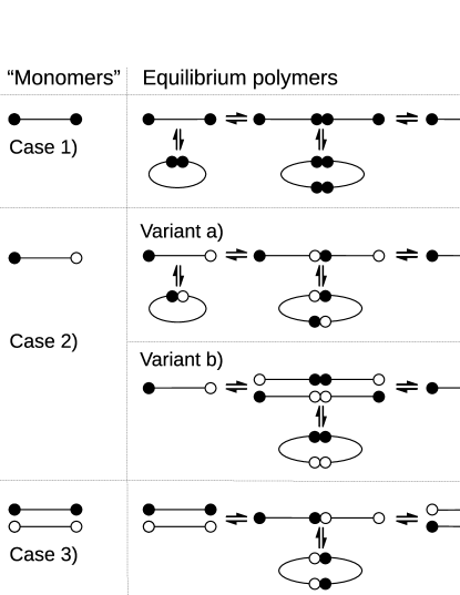
Figure 1: The three classical cases of linear polymerization discussed in Ref. (Jacobson and Stockmayer, 1950) that involve only two different reactive groups and no more than two different macromonomers. Reactive groups of a different type are displayed by different beads. The different macromonomers on the left assemble into linear and cyclic molecules where the simplest ones are shown on the right.

An irreversible alternating co-polymerization without loop formation was partially treated in Flory’s original work (Flory, 1936) on condensation polymerization omitting a computation of the weight averages and polydispersity of both, the differently terminated chains and the full sample. A later attempt to provide the missing averages (Mizerovskii and Padokhin, 2013) was not successful, as discussed in the Appendix. Furthermore, weight distributions and averages for case 2b without loop formation were not discussed in literature to the best of our knowledge. We close this gap by deriving the corresponding distributions and averages for the loop free limit in the Appendix.

With consideration of loop formation, case 3 was discussed only for stoichiometrically balanced systems or completely reacted minority species in the original work of JS (Jacobson and Stockmayer, 1950). One may recall here also the limitations of the the JS approach, that provides no quantitative prediction for conversion, etc., see Ref. (Lang and Kumar, 2021) for a more detailed discussion. Random co-polymerization in the presence of cyclization has been discussed by Szymanski (Szymanski, 1989, 1992) without covering the case of an alternating co-polymerization. Vermonden et al. (Vermonden et al., 2003) applied the JS model to case 3, addressing ring-chain equilibria in strictly alternating systems of water soluble coordination polymers. Here, the second ligand complex with a metal ion yields a different binding energy, which leads to asymmetric results that can be modeled as a first shell substitution effect. Note that the treatment by Vermonden et al. (Vermonden et al., 2003) is based upon sample average probabilities. However, cyclic molecules with an alternating sequence of building block have always a balanced stoichiometry, see section Alternating co-polymerization (case 3). Deviations from stoichiometry are balanced within the linear species alone. Therefore, the treatment in Ref. (Vermonden et al., 2003) is only approximate and becomes increasingly inaccurate for an increasing weight fraction of rings or stoichiometric imbalance. To the best of our knowledge, there is no accurate and self-consistent treatment of case 2b and 3 available in literature no matter whether cyclization is included or not. It is the aim of the present paper, to provide this treatment in its simplest form focusing on linear Gaussian strands (LGS) as basic building blocks and using Flory’s simplifying assumption of equal reactivity of reactive groups of the same kind and independence of reactions.

In the following sections, we extend the approach of Ref. (Lang and Kumar, 2021) to case 2b and case 3, whereby we start with the latter to simplify the discussion. We use the numerical scheme that is explained in the appendix of Ref. (Lang and Kumar, 2021) to obtain exact numerical solutions of the set of balance equations. Note that an example for this scheme is given in the SI of Ref. (Lang and Kumar, 2021). Also, the second section of Ref. (Lang and Kumar, 2021) is a useful introduction for our approach, since it contains the basic expressions for intra- and intermolecular reactions, the law of mass action, and the balance equations that are applied below. All key findings related to weight fractions of rings or weight distributions of rings and linear chains are tested by Monte Carlo simulations. These are also described in the Appendix of Ref. (Lang and Kumar, 2021).

II Alternating co-polymerization (case 3)

Let us consider the case of an alternating polymerization where $2$-functional strands of type $A$ react exclusively with $2$-functional strands of type $B$. Let

$$r=\frac{c_{\text{A}}}{c_{\text{B}}}$$ (1)

denote the stoichiometric ratio of the concentrations of reactive groups, $c_{\text{A}}$ and $c_{\text{B}}$, of strands of type $A$ and $B$ respectively. The total concentration of reactive groups is here

$$c_{\text{t}}=c_{\text{A}}+c_{\text{B}}=c_{\text{B}}\left(r+1\right).$$ (2)

Once $r\neq 1$ for irreversible systems, one typically assumes that the minority species is converted completely, while non-reacted groups are located exclusively on the majority species (Suckow et al., 2019). For reversible systems, such an assumption is not feasible as unbound groups are continuously created by bond breaking. Without loss of generality, let us choose $A$ as the minority component, which restricts our discussion to $r<1$. We further simplify the discussion by assuming that the strands $A$ and $B$ are identical except for the end groups, so that both strands occupy roughly the same volume.

To proceed, we require the number fraction distribution of linear species with an even number of strands, since only these can form loops in an alternating co-polymerization. Virtually all treatments of linear or non-linear co-polymerization do not distinguish between chains with an even or odd number of strands. Instead, they focus mainly on average molecular weights, as these are easier to derive, see e.g. (Stockmayer, 1944; Flory, 1946, 1953; Macosko and Miller, 1976). The only exceptions we could find are Refs. (Flory, 1936; Mizerovskii and Padokhin, 2013). Even there, not all required distributions and averages are available. Quite surprisingly, none of these works provides a correct set of equations for the number and weight distributions as can be shown by checking for normalization. Therefore, we added section Case 3 without rings to the Appendix, where we present a complete derivation of all required distributions and averages.

To model cyclization, we must distinguish the chains regarding their ends. We call chains “$A$-terminated”, if two $A$ strands are on their ends, “$B$ terminated” chains have two ends of type $B$, while “$m$-terminated” chains have end groups of both types. We use an index $A$, $B$, or $m$ to indicate that a distribution or averages refers to one of these particular classes of chains. Weight fractions are denoted as w, while number fractions are denoted by $n$. Thus, $\text{w}_{\text{A}}$ is the weight fraction of $A$-terminated chains, while $n_{\text{m}}$ is the number fraction of mixed terminated chains, as an example. Below, we use also a second kind of weight fractions $\text{w}_{\text{j}}$ where $j=0,1,2$ counts the number of bound reactive groups (“closed stickers” (Stukhalin et al., 2013)) of the strands. For distinction, the total weight fraction of loops is denoted by $\omega$ while weight fractions of loops made of $k$ strands is written as $\omega_{\text{k}}$. Finally, $\omega_{\text{A}}$ is the weight fraction of $A$ strands that are part of loops.

In case of loop formation, the loops are always at 100% conversion, contain an even number of strands, and must be stoichiometrically balanced due to the alternating scheme of case 3. Similar to equation (16) of Ref. (Lang and Kumar, 2021), loop formation reduces the conversion, $p$, inside the linear chain species to

$$p_{\text{lin}}=\frac{p-\omega_{\text{A}}}{1-\omega_{\text{A}}}.$$ (3)

Furthermore, the stoichiometric balance of the loops, shifts the stoichiometric ratio of the linear fraction to

$$r_{\text{lin}}=\frac{r\left(1-\omega_{\text{A}}\right)}{1-r\omega_{\text{A}}}.$$ (4)

Note that $\omega_{\text{A}}$ enters here in both equations above instead of $\omega$ that was used in Ref. (Lang and Kumar, 2021), since the total weight fraction of loops is limited by the weight fraction of the minority species $A$.

Both $p_{\text{lin}}$ and $r_{\text{lin}}$ describe the properties of the linear chain fraction in the presence of loops, and replace $p$ and $r$ in all equations that are taken from section Case 3 without rings of the Appendix. To clarify this point in our notation, we add to all quantities taken from the Appendix the additional suffix “lin”. Furthermore, we have computed all weight fractions $\text{w}_{\text{X}}$ with $X=A,B,m,...$ etc. in section Case 3 without rings in the absence of loops. Normalization of these quantities with respect to the full sample is obtained by multiplication with $1-\omega$.

We proceed as in Ref. (Lang and Kumar, 2021) by proposing balance equations for $\text{w}_{\text{j}}$. Since any reaction of an $A$ group involves a reaction of a $B$ group, it is sufficient to write down the balance equations only in terms of the $A$ groups skipping an additional suffix $A$ for all $\text{w}_{\text{j}}$. The weight fraction of non-reacted $A$ strands, $\text{w}_{0}$, must be part of the weight fraction of linear chains, $1-\omega$, and is given by

$$\text{w}_{0}=\text{w}_{\text{\text{A,0}}}\left(1-\omega\right)=\frac{r_{\text{lin}}\left(1-p_{\text{lin}}\right)^{2}}{1+r_{\text{lin}}}\left(1-\omega\right),$$ (5)

see equation (A26) of the Appendix for $\text{w}_{\text{A,0}}$.

For the balance equation of strands $\text{w}_{1}$ with strands $\text{w}_{0}$, we have to consider that the concentration of reaction partners of type $B$ is $\left(1-rp\right)c_{\text{B}}$. Furthermore, there are two chain ends of $\text{w}_{0}$ that can react, while the law of mass action, equation (A7), does not contribute another factor of two in contrast to case 1 or 2b. Altogether, we obtain

$$\text{w}_{\text{1}}=2Kc_{\text{B}}\left(1-rp\right)\text{w}_{0}=\frac{2Kc_{\text{t}}}{r+1}\left(1-rp\right)\text{w}_{0}.$$ (6)

Regarding the balance between $\text{w}_{2}$ and $\text{w}_{1}$, we consider first only those forward reactions that do not lead to cyclization and only backwards reactions where no cyclic molecule transforms into a linear chain. Therefore, we put only the weight fraction of $A$ strands that are not in cycles on the left hand side, $\text{w}_{2}-\omega_{\text{A}}$, together with a symmetry factor of two that reflects that each strand $\text{w}_{2}$ contributes to two bonds that can break, while only one reactive group of $\text{w}_{1}$ can form bonds. In analogy to equation (15) of Ref. (Lang and Kumar, 2021), we obtain

$$2\left(\text{w}_{2}-\omega_{\text{A}}\right)=Kc_{\text{B}}\left(1-rp\right)\text{w}_{\text{1}}=\frac{Kc_{\text{t}}}{\left(r+1\right)}\left(1-rp\right)\text{w}_{\text{1}}.$$ (7)

Loop formation of the smallest ring does not couple to $w_{0}$ as in case 1 polymerization, instead, it couples to the concentration of dimers. These establish a weight fraction of

$$\text{w}_{\text{m,0,lin}}=\frac{4r_{\text{lin}}p_{\text{lin}}\left(1-p_{\text{lin}}\right)\left(1-r_{\text{lin}}p_{\text{lin}}\right)}{1+r_{\text{lin}}}\left(1-\omega\right)$$ (8)

among all molecules, see equation (A25).

The concentration of the second dimer end next to the first is $2^{-3/2}c_{\text{i}}$. Here, $c_{\text{i}}$ is the concentration of the second end around the first of a single LGS, see equation (10) for $f=2$ of Ref. (Lang and Kumar, 2021). Since there are two bonds per cyclic dimer that can break, we obtain for the weight fraction of the smallest loop the balance equation

$$2\omega_{1}=2^{-3/2}c_{\text{i}}K\text{w}_{\text{m,0,lin}}.$$ (9)

In total, this leads to an extra coefficient of $2^{-1/2}$ for $\omega_{1}$ as compared to case 1. Longer chains that can form loops contain $z$ additional pairs of $A$ and $B$ strands as compared to the dimer, and they exist with a reduced probability $\left(r_{\text{lin}}p_{\text{lin}}^{2}\right)^{z}$, see section Case 3 without rings. As for case 1 discussed in Ref. (Lang and Kumar, 2021), this leads to a total weight fraction of $A$-mers in the loops that is a function of the smallest loop, $\omega_{1}$,

$$\omega_{\text{A}}=\frac{\omega_{1}}{2}\sum_{z=1}^{\infty}z^{-3/2}\left(r_{\text{lin}}p_{\text{lin}}^{2}\right)^{z-1}.$$ (10)

The extra coefficient of $1/2$ in this equation reflects the fact that only one half of all strands in the loop is of type $A$. The total weight fraction of loops among all $A$ and $B$ strands is therefore

$$\omega=\frac{2\omega_{A}}{1+r}.$$ (11)

In the limit of $c_{\text{t}}\gg c_{\text{i}}$ and $K\rightarrow\infty$ where $r_{\text{lin}}p_{\text{lin}}^{2}\rightarrow 1$, we obtain for $r=1$ a shift of the critical concentration, $c_{\text{crit}}$, by a factor of $2^{-1/2}$ towards smaller concentrations as compared to case 1,

$$c_{\text{crit}}=2^{-1/2}\sum_{z=1}^{\infty}z^{-3/2}c_{\text{i}}.$$ (12)

This shift results from a factor of $2^{-3/2}$ due to end-contacts of dimers instead of monomers and a factor of 2 for $r=1$ regarding the concentration of possible reaction partners. The number density of loops per strand is

$$n_{\text{L}}=\frac{\omega_{1}}{2\left(1+r\right)}\sum_{z=1}^{\infty}z^{-5/2}\left(r_{\text{lin}}p_{\text{lin}}^{2}\right)^{z-1},$$ (13)

which provides the number average degree of polymerization (DP) of the loops through

$$N_{\text{n,loops}}=\frac{\omega}{n_{\text{L}}}.$$ (14)

As discussed in Ref. (Lang and Kumar, 2021), the above equations together with the normalization of $\text{w}_{\text{j}}$ and the definition of $p$ given in the Appendix of Ref. (Lang and Kumar, 2021) allow to solve the set of balance equations numerically. With the solution of these equations, $\omega_{\text{A}}$ and $p$ become available, which is the basis for computing the missing distributions and averages of linear chains as described below for arbitrary $p$ and $r$. This provides a significant advancement as compared to previous work. JS (Jacobson and Stockmayer, 1950) discuss case 3 polymerization only in the limits of a) $r=1$ while $p\neq 1$ and b) $p=1$ while $r\neq 1$. Vermonden et al. (Vermonden et al., 2003) apply the JS model to water soluble coordination polymers. Similar to JS, these authors do not consider that ring formation reduces the conversion in the linear chain fraction and that ring formation increases the stoichiometric imbalance of the linear chains, see e.g. equation (7) of Ref. (Vermonden et al., 2003), where only sample average quantities ($p$ and $q$ in their notation) enter. This neglect allows to solve the set of equations without a recursion, but affects the accuracy of their model once a significant amount of rings is formed or a significant stoichiometric imbalance is obtained.

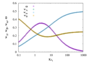
Figure 2: Weight fractions of $A$, $B$, and $m$-terminated chains, and loops for $c_{\text{i}}=10^{-2}$ as a function of $Kc_{\text{t}}$ for stoichiometric ratio $r=1.0$ and $K=10^{3}$. Symbols refer to simulation data, lines are numerical solution of the balance equations for case 3.

For the presentation of the most relevant dependencies on reaction constant(s) and concentrations, we have chosen a similar parameter range as in our preceding work (Lang and Kumar, 2021), see the detailed discussion there. In experiments, the reaction constant can be adjusted with the temperature of the sample, see equation (24) of Ref. (Lang and Kumar, 2021), or by choosing a different chemistry for the reactive groups. However, care needs to be taken here as many physical parameters (interactions between the molecules, viscosity, …) are a function of temperature. The temperature dependence of these parameters might interfere largely with the desired modification of the reaction constant.

The weight fractions of $A$, $B$, $m$-terminated chains and the weight fraction of loops are shown in Figure 2. In marked contrast to case 1 polymerization, see Ref. (Lang and Kumar, 2021), there is a maximum of loop formation that precedes the maximum ($r<1$) or the approach of saturation ($r=1)$ of the weight fraction of the mixed terminated chains

$$\text{w}_{\text{m}}=\frac{4r_{\text{lin}}p_{\text{lin}}(1-p_{\text{lin}})(1-r_{\text{lin}}p_{\text{lin}})}{\left(1+r_{\text{lin}}\right)\left(1-r_{\text{lin}}p_{\text{lin}}^{2}\right)^{2}}\left(1-\omega\right)$$ (15)

for increasing $Kc_{\text{t}}$, since loops are derived predominantly from the shortest chains of $\text{w}_{\text{m}}$. These shortest chains are dimers containing one intermolecular bond that disassembles in the limit of very low concentration. On the other hand, the probability for loop formation decreases in the limit of high concentrations. In between these limits, there is an optimum concentration for loop formation regarding the weight fraction of loops (but not regarding the total weight of loops in the sample, see section Discussion).

In Figure 2, the data for $\text{w}_{\text{A}}$ and $\text{w}_{\text{B}}$ coincide due to symmetry. This Figure shows also that the limit of low concentrations, $c_{\text{t}}\rightarrow 0$, refers to the limit of $p\rightarrow 0$, where isolated linear macromonomers of both types dominate the weight distribution, $\text{w}_{\text{A}},\text{w}_{\text{B}}\rightarrow 1/2$. In the opposite limit of $c_{\text{t}}\gg 0$, there is $p\rightarrow 1$ and $\omega\rightarrow 0$ such that long linear chains dominate leading to a random distribution of chain ends: $\text{w}_{\text{m}}\rightarrow 1/2$ and $\text{w}_{\text{A}},\text{w}_{\text{B}}\rightarrow 1/4$.

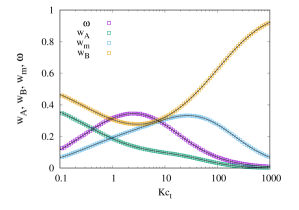
Figure 3: Weight fractions of $A$, $B$, and $m$-terminated chains, and loops for same parameters as in Figure 2 except of $r=0.8$).

In Figure 3, we show the weight fractions of $A$, $B$, $m$-terminated chains and loops for the same parameters as in Figure 2 except of a small stoichiometric imbalance, $r=0.8$. This imbalance lets the majority species of reactive groups dominate chain termination in the high concentration limit, $c_{\text{t}}\gg 0$, where other chain types are increasingly suppressed. Since loop formation requires mixed terminated chains, the disappearance of the latter reduces also the weight fraction of loops.

Let us use the weight fraction of dimers, equation (8), as a simple, rough estimate of the location of the maximum weight fraction of loops through

$$\frac{\text{d}\text{w}_{\text{m,0,lin}}}{\text{d}p_{\text{lin}}}=0,$$ (16)

since the weight fraction of loops is dominated by the smallest loops. This condition leads to the equation

$$1-2r_{\text{lin}}p_{\text{lin}}-2p_{\text{lin}}+3r_{\text{lin}}p_{\text{lin}}^{2}=0$$ (17)

where only the negative branch of the solutions

$$p_{\text{opt}}\approx\frac{r_{\text{lin}}+1\pm\sqrt{r_{\text{lin}}^{2}-r_{\text{lin}}+1}}{3r_{\text{lin}}}$$ (18)

serves as an estimate for the conversion at the maximum amount of loops, since the positive branch is $>1$ for all $r_{\text{lin}}<1$. In the example of Figure 2 with $r=0.8$, a maximum weight fraction of $\approx 34.4\%$ of loops is obtained roughly at $c_{\text{t}}\approx c_{\text{i}}/4$, resulting in a conversion $p\approx 0.64$ for $K=10^{3}$. Both $p$ and $\omega$ are clearly smaller at the maximum as in case 1 polymerization for the same set of concentrations and reaction constant.

Let us now compute the number fractions $n_{\text{x}}$ of the different species inside the full sample. Recall that the number fractions $n_{\text{x}}$ of section Case 3 without rings are normalized to unity within the linear chain fraction. In order to obtain properly normalized number fractions within the full sample, we consider first the average DP of the linear chains,

$$N_{\text{n,lin}}=\frac{1+r_{\text{lin}}}{1+r_{\text{lin}}-2r_{\text{lin}}p_{\text{lin}}},$$ (19)

see equation (A11). The number density of linear chains per strand is

$$n_{\text{C}}=\left(1-\omega\right)/N_{\text{n,lin}},$$ (20)

which we use to compute the number fraction of rings among all molecules,

$$n_{\text{loops}}=\frac{n_{\text{L}}}{n_{\text{C}}+n_{\text{L}}}.$$ (21)

As mentioned above, the equations in section Case 3 without rings for the linear species can be used after replacing all $p$ and $r$ by $p_{\text{lin}}$ and $r_{\text{lin}}$ respectively, while all number fractions need to be multiplied by $1-n_{\text{loops}}$ and all weight fractions by $1-\omega$. Thus, our approach provides exact numerical solutions for all number fractions, weight fractions, and distributions.

As for case one, see Ref. (Lang and Kumar, 2021), we can use these results to obtain sample average quantities that might be useful for an analysis of the reactions. For instance, both $n_{\text{C}}$ and $n_{\text{L}}$ set up the total density of molecules among the total number of strands, thus, they are related to the sample average DP via

$$\frac{1}{N_{\text{n}}}=n_{\text{C}}+n_{\text{L}}$$ (22)

$$=\frac{\left(1-\omega\right)\left(1+r_{\text{lin}}-2r_{\text{lin}}p_{\text{lin}}\right)}{1+r_{\text{lin}}}+\frac{\omega}{N_{\text{n,loops}}}.$$

Similarly, the weight average DP can be obtained by a weighted average of the four contributions due to rings, and $A$, $B$, and $m$ terminated chains. The resulting expressions are readily obtained following the corresponding steps discussed for case 1 in Ref. (Lang and Kumar, 2021), but they are quite lengthy. Therefore, we omit an explicit treatment of these equations here. Instead, we show the resulting data in several Figures.

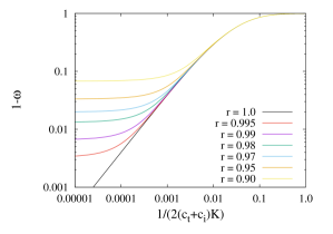
Figure 4: Weight fraction of linear chains, $1-\omega$, as a function of $K$ for $c_{\text{t}}=c_{\text{i}}/10$ and $c_{\text{i}}=1/10$ for stoichimetric ratios close to $r=1$ (case 3).

In Figure 4, we show the weight fraction of linear chains, $1-\omega$, as a function of $K$ and dilute concentrations $c_{\text{t}}=c_{\text{i}}/10$ where the limit $K\rightarrow\infty$ at $r=1$ provides a weight fraction of 100% rings. As expected, any small stoichiometric imbalance induces a non-zero weight fraction of linear chains that is somewhat larger than the lower bound estimate $\left(1-r\right)/\left(1+r\right)$ (all minority species in rings and no polymerization of chains) for the weight fraction of linear chains of in the limit of $K\rightarrow\infty$. Altogether, Figure 4 demonstrates that a 100% weight fraction of rings is reached only for $r=1$.

In real systems, composition fluctuations arising from the stochastic motion of the unsaturated reactive groups will control the weight fraction of rings that can be reached for $r\approx 1$ in the limit of large $K$. For irreversible recombination similar to our case 3, it is well established (Ovchinnikov and Zeldovich, 1978; Toussaint and Wilczek, 1983; Kang and Redner, 1984) that these dominate the long time reaction kinetics close to stoichiometrically balanced conditions, $r\approx 1$. A similar dominance of diffusion and composition fluctuations has been found also for reversible systems (Rey and Cardy, 1999; Gopich et al., 2001), slowing down the convergence towards complete conversion. Significant diffusion effects are also in conflict with the assumption of an independence of all reactions, since diffusion control leads inevitably to higher reaction rates for the faster moving smaller molecules. Therefore, we expect that the computations of this section are reasonable approximations for the reaction controlled limit only up to a limiting $K$ where composition fluctuations or diffusion effects come into play. Deeper insight into this complex problem could be obtained with suitable Monte-Carlo or molecular dynamics simulations as these allow to keep track of the weight dependent mobility of the molecules including a possible impact of entanglements on polymerization.

One subtle point in this discussion concerns rings having always $r=1$, so that the linear chains must compensate all of the stoichiometric imbalance. Any composition fluctuation, thus, reduces both the weight fraction of rings and the DP of the chains by an amount proportional to the fluctuating average composition difference in the system. In our computations, this could be taken into account by replacing the true $r$ by an effective $r$ that is a function of the particular reaction constant, since increasing $K$ drives the effective $r$ to unity. However, the details of such a process have not been elaborated yet for a polymer model system where additional couplings between the system parameters arise (e.g. the composition fluctuations couple to the overlap of polymer molecules and the weight fraction of the rings).

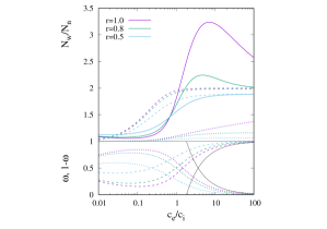
Figure 5: Weight fraction of rings and chains (lower part) and polydispersity (upper part) at an intermediate reaction constant $K=10^{4}$ at $c_{\text{i}}=10^{-2}$, for a range of stoichiometric imbalances $r$. Upper part: the continuous lines address the sample average polydispersity, the dashed lines the polydispersity of the dominating (for $r\neq 1$) odd chains with end groups of either type $A$ or $B$, respectively. The dotted lines show the polydispersity of the rings. Lower part: weight fractions of chains (dashed lines) and rings (dotted lines). The black line corresponds to the limit of $K\rightarrow\infty$.

The polydispersity of the full sample, of odd numbered chains, and the rings is shown in Figure 5 for a range of stoichiometric imbalances around $r=1$. The general trend is that an increasing stoichiometric imbalance limits the average degrees of polymerization of both linear chains and rings for $c_{\text{t}}\gtrsim c_{\text{i}}$ and thus, it limits the difference in the molecular weights between these fractions. This leads to a decreasing peak in polydispersity for a decreasing $r<1$. This trend is reversed for the low concentration regime, $c_{\text{t}}\lesssim c_{\text{i}}$, since there, increasing the stoichiometric imbalance is equivalent to introducing larger portions of non-reacted monomer strands that are shorter than any ring in the system, which increases polydispersity. Qualitatively similar to case 1, the DP of the chains grows quickly prior to the critical concentration (polydispersity approaches two), while the polydispersity of the sample reaches its maximum significantly after the critical concentration. Thus, a significant number fraction of the linear chains needs to develop first until a high polydispersity is reached at concentrations clearly beyond the critical concentration.

For intermediate reaction constants, a peak develops for the weight fraction of the rings as discussed above, see Figure 5. This peak turns into a broad plateau in the limit of large $K$. The Figure shows also the shift of the critical concentration by a factor of $2^{-1/2}$ as compared to case 1 (see equation (12).

With Figure 6, we compare the impact of stoichiometric ratio and reaction constant $K$ on the polydispersity. For this example, we focus on $c_{\text{e}}/c_{\text{i}}=4$, which is in the range of the polydispersity peaks of Figure 5. Recall that a high polydispersity requires the coexistence of short cyclic and long linear molecules at largely different degrees of polymerization and at a significant weight fraction of the linear chains, which is why polydispersity is largest for concentrations somewhat larger than $c_{\text{crit}}$. The main impact of increasing $K$ is to enforce chain growth, which is not limited by stoichiometric conditions for $r=1$. For stoichiometric imbalance, $r<1$, there is a particular reaction constant, where chains are terminated equivalently due to missing bonds and due to excess majority strands. This point is roughly visible in Figure 6 by the point where data for a larger reaction constant than a particular $K$ separate towards a larger polydispersity, i. e. a larger DP of the linear chains. At an $r$ below the separation point, the data for the corresponding reaction constants are dominated by the stoichiometric condition. At large $r$ close to unity, the impact of a large $K$ stands out for a broad range of reaction constants and leads to a large increase of polydispersity (DP of the linear chains) as a function of $K$.

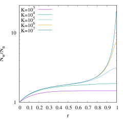
Figure 6: Polydispersity as a function of stoichiometric ratio $r$ and reaction constant $K$ (case 3) at $c_{\text{e}}/c_{\text{i}}=4$.

This latter observation could be used to check the preparation conditions and the quality of the macromonomers, since any impurity, missing, or inactive group will shift the maximum away from $r=1$, if the there are more defects in one of the species as compared to the other. If a similar amount of defects arises within both types of macromonomers, still the DP of the linear chains might stagnate for an increasing $K$, which could be traced by analyzing related quantities like, for instance, the viscosity of the supramolecular solution or melt.

III $AB$ monomers with two orthogonal reactions (case 2b)

For case 2b, the same $A-B$ monomers form only bonds between two $A$ groups or between two $B$ groups, like the supramolecular polymers of Ref. (Gröger et al., 2011). The weight distributions of case 2b are similar to the weight distributions of case 3 polymerization for a stoichiometric ratio $r=1$. However, there are now two different types of “dimers” with either $A$ or $B$ groups on their ends that can form the smallest possible loops, see Figure 1. The conversions of these groups, $p_{\text{A}}$ and $p_{\text{B}}$, may differ significantly, $p_{\text{A}}\neq p_{\text{B}}$. Furthermore, the concentration of $A$ and $B$ groups is $c_{\text{A}}=c_{\text{B}}=c_{\text{t}}/2$ where $c_{\text{t}}$ is the concentration of all reactive groups. These deviations from case 3 cause significant quantitative and qualitative modifications that require an explicit discussion.

We consider that conversions $p_{\text{A}}$ and $p_{\text{B}}$ of the $A$ and $B$ groups are independent from each other and given by the corresponding law of mass action, equation (A41). As for case 3, the strands in the loops are at 100% conversion, and we have to renormalize the conversions $p_{\text{X}\text{,lin}}$ of the reactive groups $X=A,B$ within the linear chain fraction for each reactive group separately:

$$p_{\text{X}\text{,lin}}=\frac{p_{\text{X}}-\omega}{1-\omega}.$$ (23)

Similar to case 3, the smallest possible loops are formed from dimers, however, there are now $A$-terminated dimers and $B$-terminated dimers that contribute to the formation of the smallest loop. For $p_{\text{A}}\neq p_{\text{B}}$, we introduce reaction constants $K_{\text{A}}$ and $K_{\text{B}}$ to describe the reversible $A$ and $B$ bonds respectively, see section Case 2b without rings of the Appendix for more details. Loop formation occurs now either by pairs of $A$ or $B$ bonds, respectively, in balance with the corresponding backwards reaction.

The weight fraction of the non-reacted monomer is

$$\text{w}_{0}=\text{w}_{\text{m,0}}\left(1-\omega\right)=\left(1-p_{\text{A,lin}}\right)\left(1-p_{\text{B,lin}}\right)\left(1-\omega\right),$$ (24)

see equation (A53) with $z=0$. Here, there are two reactions with $A$ and $B$ groups respectively, leading to the formation of strands with one reacted group, $\text{w}_{1}$. For this particular case, however, we must distinguish these as $\text{w}_{1,\text{A}}$ and $\text{w}_{1,\text{B}}$ where the suffix indicates the type of the reacted end group. Thus,

$$\text{w}_{\text{1,A}}=c_{\text{A}}\left(1-p_{\text{A}}\right)K_{\text{A}}\text{w}_{0}.$$ (25)

$$\text{w}_{\text{1,B}}=c_{\text{B}}\left(1-p_{\text{B}}\right)K_{\text{B}}\text{w}_{0}.$$ (26)

$$\text{w}_{\text{1}}=\text{w}_{1,\text{A}}+\text{w}_{1,\text{B}}.$$ (27)

These two types of $\text{w}_{1}$ strands lead to the formation of $\text{w}_{2}$ strands that are not part of any loop. In analogy to equation (7), we obtain

$$2\left(\text{w}_{2}-\omega\right)=c_{\text{A}}\left(1-p_{\text{A}}\right)K_{\text{A}}\text{w}_{\text{1,B}}+c_{\text{B}}\left(1-p_{\text{B}}\right)K_{\text{B}}\text{w}_{\text{1,A}}.$$ (28)

Note that the above balance equations allow to compute the conversion of species $X=A,B$ through

$$p_{\text{X}}=\text{w}_{2}+\text{w}_{1,\text{X}}.$$ (29)

The weight fraction of the smallest loop, $\omega_{1}$, couples to the weight fractions of the smallest $A$ and $B$ terminated molecules,

$$\text{w}_{\text{A,0,lin}}=p_{\text{B,lin}}\left(1-p_{\text{A,lin}}\right)^{2}\left(1-\omega\right)/2$$ (30)

and

$$\text{w}_{\text{B,0,lin}}=p_{\text{A,lin}}\left(1-p_{\text{B,lin}}\right)^{2}\left(1-\omega\right)/2$$ (31)

respectively, see equation (A51) and (A52) and Figure 1. The smallest loop is a dimer where two bonds can break. This leads to the balance equation

$$2\omega_{1}=2^{-3/2}c_{\text{i}}\left(K_{\text{A}}\text{w}_{\text{A,0,lin}}+K_{\text{B}}\text{w}_{\text{B,0,lin}}\right)$$ (32)

for the smallest loop and a total weight fraction of loops of

$$\omega=\omega_{1}\sum_{z=1}^{\infty}z^{-3/2}\left(p_{\text{A,lin}}p_{\text{B,lin}}\right)^{z-1}.$$ (33)

In total, we obtain in the limit of $c_{\text{t}}\gg c_{\text{i}}$ and $K_{\text{X}}\rightarrow\infty$ where $p_{\text{A,lin}}p_{\text{B,lin}}\rightarrow 1$ that $\omega$ remains smaller than in case 1 by a factor of $2^{1/2}$ similar to case 3 for $r=1$. As before, the above set of equations can be solved exactly using the numerical scheme discussed in the Appendix of Ref. (Lang and Kumar, 2021).

With these equations solved, we proceed to the computation of the distribution functions and averages. Here, we require the number density of loops per initial strand,

$$n_{\text{L}}=\frac{\omega_{1}}{2}\sum_{z=1}^{\infty}z^{-5/2}\left(p_{\text{A,lin}}p_{\text{B,lin}}\right)^{z-1},$$ (34)

and the average DP of the loops that is computed using equation (14). The factor $1/2$ in equation (34) takes into account that loops are formed by pairs (or multiple pairs) of $A-B$ strands. The average DP of the linear chains is given by equation (A44) after replacing $p_{\text{A}}$ and $p_{\text{B}}$ with the corresponding expressions of the linear chain fraction, $p_{\text{A,lin}}$ and $p_{\text{B,lin}}$. Finally, the number density of chains per strand, $n_{\text{C}}$, and the number fraction of loops among all molecules, $n_{\text{loops}}$, are computed with equation (20) and (21).

After these results have been obtained, the number and weight fractions of the linear chains of section Case 2b without rings must be normalized by a factor $1-n_{\text{loops}}$ and $1-\omega$, respectively, to reflect the corresponding contributions to the full sample similar to the preceding section. Here, again $p_{\text{A,lin}}$ and $p_{\text{B,lin}}$ replace $p_{\text{A}}$ and $p_{\text{B}}$ in all expressions. Either through the resulting number and weight distributions or by combining the corresponding averages as we have done in the preceding section and in Ref. (Lang and Kumar, 2021), the sample wide number average and weight average DP becomes available. We do not provide explicit equations here, since the corresponding steps have been discussed previously, the derivation is straightforward, and the resulting expressions are quite lengthy. As before, we provide Figures with the resulting data for a range of reaction constants and concentrations.

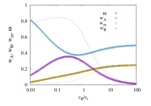
Figure 7: Weight fractions $\text{w}_{\text{A}}$, $\text{w}_{\text{B}}$, $\text{w}_{\text{m}}$, and $\omega$ for $K_{\text{A}}=K_{\text{B}}=100$ (symbols for simulation data and continuous lines for theory) and $c_{\text{i}}=10^{-2}$ (case 2b). Dashed lines represent theory for $K_{\text{A}}=K_{\text{B}}=1000$ to indicate the trend as a function of increasing $K$.

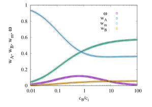
Figure 8: Weight fractions $\text{w}_{\text{A}}$, $\text{w}_{\text{B}}$, $\text{w}_{\text{m}}$, and $\omega$ for $K_{\text{A}}=100$, $K_{\text{B}}=1000$, and $c_{\text{i}}=10^{-2}$ (case 2b).

We have tested our equations by comparing the exact numerical solution of the balance equations with Monte Carlo simulation data. Figure 7 provides the corresponding data for the weight fractions of $A$, $B$, and $m$-terminated chains of symmetric cases at different reaction constants. Similar to case 3, the limiting case of $c_{\text{B}}\rightarrow 0$ provides the distributions of the macromonomers without reactions, which is $\text{w}_{\text{m}}\rightarrow 1$, while all other contributions decay to zero. Again, the limit of $Kc_{\text{B}}\rightarrow\infty$ produces no rings but infinitely long chains with a random distribution of ends $\text{w}_{\text{m}}\rightarrow 1/2$, and $\text{w}_{\text{A}},\text{w}_{\text{B}}\rightarrow 1/4$. Between these limits, a significant or even dominant portion of rings is being formed that increases with increasing reaction constant $K$. As for case 3, the optimum conditions for ring formation can be estimated by analyzing the maximum of the dimers, which contains here two contributions and is more complex to analyze. For the sake of brevity, we omit an explicit discussion here and mention that this peak turns into a broad plateaux with $\omega\approx 1$ for $c_{\text{B}}<c_{\text{i}}$ and $c_{\text{B}}K\gg 1$ in similar manner as for case 2b.

Figure 8 shows data for an asymmetric case with a smaller reaction constant $K_{\text{A}}$. Here $A$ groups predominantly terminate chains, once these grow for $Kc_{\text{A}}>1$. This reduces significantly the fraction of loops together with the DP of the linear chains and loops.

In Figure 9, we show the weight fractions of loops and chains (bottom) along with the polydispersity of the sample for a range of different $K_{\text{B}}$ at a fixed $K_{\text{A}}$. The qualitative behavior is quite similar to case 3 at a significantly reduced weight fraction of loops and degrees of polymerization similar to the preceding Figure. The polydispersity peak of the sample is reached at significantly larger concentration as the critical concentration. The critical concentration itself is shifted by a factor of $2^{1/2}$ to lower concentrations as compared to case 1, again in accord with case 3 for $r=1$. Another interesting point is that the weight distributions of this case are similar to $r=1$ of case 3. However, composition fluctuations of reactive groups are largely suppressed here, and they couple to the concentration fluctuations of the polymers on large length scales.

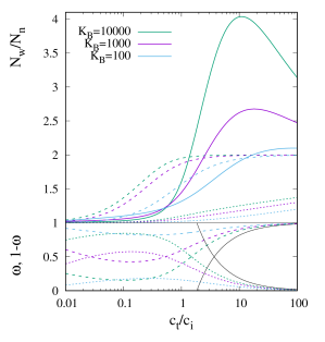
Figure 9: Weight fractions of loops and polydispersities for $K_{\text{A}}=10^{4}$ and $c_{\text{i}}=10^{-2}$ as a function of the total concentration of reactive groups, $c_{\text{t}}$, for different $K_{\text{B}}$ (case 2b).

IV Discussion

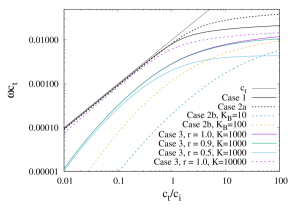
Figure 10: Weight fraction of loops in total sample including a solvent of same density for different model systems with $K=K_{\text{A}}=10^{3}$ (unless indicated otherwise) and $c_{\text{i}}=10^{-2}$.

Let us start our with a quantitative comparison of loop formation in all cases discussed in the preceding sections and in Ref. (Lang and Kumar, 2021). This comparison is shown in Figure 10 using the same representation of the data as in the work of Ercolani (Ercolani et al., 1993) for a better comparison with preceding work. For our discussion, we have also compiled the balance equations and critical concentrations in table 1. In Figure 10, we have multiplied the weight fraction of loops with the total concentration of reactive groups, $c_{\text{t}}$, which is proportional to the concentration of macromonomers. If the solvent has the same density as the macromonomer, the $y$-axis is equivalent to the weight fraction of rings in the total sample. For comparison, $c_{\text{t}}$ is included referring to $\omega=1$. In the low concentration regime, $c_{\text{t}}<c_{\text{i}}$, the weight fraction of loops is essentially the weight fraction of the macromonomers for case 1 and case 2a, settling to an almost constant amount of rings around the critical concentration. As discussed above, the cross-over occurs later for case 2a, leading to about twice as much rings in the high concentration limit. Small differences between case 1 and 2 in the low concentration limit result from a different conversion because either $K$ or $2K$ enters in the law of mass action. The Figure contains also one example of case 3 at $r=1$ and a “high” reaction constant $K=10^{4}$. This cases settles at a lower amount of loops by a factor of $2^{-1/2}$, which stems from a lower critical concentration, see Table 1. Thus, the dependence of the uppermost three sets of data demonstrates that nature prefers to make loops in the large $K$ limit for concentrations up to $c_{\text{crit}}$, while for $c>c_{\text{crit}}$, the excess concentration of macromonomers beyond $c_{\text{crit}}$ is predominantly converted into linear chains.

	case 1	case 2a	case 2b	case 3
$w_{1}$	$4\left(1-p\right)c_{\text{t}}K\text{w}_{0}$	$\left(1-p\right)c_{\text{t}}K\text{w}_{0}$	$\left[\left(1-p_{\text{A}}\right)c_{\text{A}}K_{\text{A}}+\left(1-p_{\text{B}}\right)c_{\text{B}}K_{\text{B}}\right]\text{w}_{0}$	$2\left(1-rp\right)\frac{c_{\text{t}}K}{r+1}\text{w}_{0}$
$\text{w}_{2}$	$4\left[\left(1-p\right)c_{\text{t}}K\right]^{2}\text{w}_{0}+\omega$	$\left[\left(1-p\right)c_{\text{t}}K\right]^{2}\text{w}_{0}/4+\omega$	$\left(1-p_{\text{A}}\right)\left(1-p_{\text{B}}\right)c_{\text{A}}c_{\text{B}}K_{\text{A}}K_{\text{B}}\text{w}_{0}+\omega$	$\left[\left(1-rp\right)\frac{c_{\text{t}}K}{\left(r+1\right)}\right]^{2}\text{w}_{\text{0}}+\omega_{\text{A}}$
$\omega$	$2c_{\text{i}}K\text{w}_{0}\sum_{k}p_{\text{lin}}^{k-1}$	$c_{\text{i}}K\text{w}_{0}\sum_{k}p_{\text{lin}}^{k-1}$	$2^{-5/2}c_{\text{i}}\left(K_{\text{A}}\text{w}_{\text{A,0,lin}}+K_{\text{B}}\text{w}_{\text{B,0,lin}}\right)\sum_{k}q^{k-1}$	$\frac{2^{-5/2}}{1+r}c_{\text{i}}K\text{w}_{\text{m,0,lin}}\sum_{k}q^{k-1}$
$c_{\text{crit}}/c_{\text{i}}$	$\sum_{k}$	$2\sum_{k}$	$2^{-1/2}\sum_{k}$	$2^{-1/2}\sum_{k}$ for $r=1$
equations	(13)-(15), (29), (30) of (Lang and Kumar, 2021)	-	(6), (7), (9), (12)	(25)-(28), (32), (33)

Table 1: Short representation of balance equations (example: $w_{1}=4\left(1-p\right)c_{\text{t}}K\text{w}_{0}$ for case 1) for $\text{w}_{1}$, $\text{w}_{2}$ and $\omega$ and the critical concentration. Equations for case 2b refer to reactions of $A$ groups only. The shorthand $\sum_{k}=\sum_{k=1}^{\infty}k^{-3/2}$ is used for all cases, while $q$ abbreviates $r_{\text{lin}}p_{\text{lin}}^{2}$ in case 2b and $p_{\text{A,lin}}p_{\text{B,lin}}$ in case 3.

For case 3 and case 2b, the weight fraction of loops is typically smaller than the total weight fraction of macromonomers in the low concentration regime for intermediate values of $K$ or $r<1$, and it must not increase linearly as shown by the data. Only for very large reaction constants and nearly stoichiometric conditions, the weight fraction of rings approaches the weight fraction of the macromonomers in the low concentration regime. Correspondingly, in the high concentration limit, the weight fraction of rings settles at lower total amounts. Off-stoichiometric conditions or a second lower reaction constant reduce sifgnificantly the portion of rings in these cases. Thus, if a high yield of rings is desired, case 2a is the best choice. If loop formation should be suppressed, case 2b is preferable, since it avoids problems related to composition fluctuations and stoichiometric balance that might arise in case 3.

The differences in the mathematical description of the four examples are highlighted in Table 1. Case 2a is - within our mean-field treatment - equivalent to case 1 except of factors of 2 regarding $K$ and $c_{\text{t}}$. The main difference between case 2b and the reference case 1 is that there are two distinct reaction mechanisms that lead to bond formation, which show up in separate contributions for $\text{w}_{1}$ and $\omega$, while $\text{w}_{2}$ results from a combination of both mechanisms. The numerical coefficient for $\omega$ highlights that loops are formed from pairs of macrmonomers, while $c_{\text{i}}$ is defined with respect to end-contacts of macromonomers. Case 3 turns into case 2a for $r=1$ regarding linear chain growth, which regards $\text{w}_{1}$ and $\text{w}_{2}$, while the difference for $\omega$ reflects that loops are formed from dimers. The probability $q$ for adding a dimer to a linear chain inside the linear fraction (case 2b and 3) takes over the role of $p_{\text{lin}}$ in case 1 and 2a, where the latter is the probability to add another monomer within the linear chain fraction there.

Figure 11 shows the concentration of loops made of $k$ strands as a function of $c_{\text{t}}$ for case 1. The data in this plot is presented in similar form as the data in Ref. (Ercolani et al., 1993) and refers to unstrained ring polymers where no additional entropic or energetic penalty applies for the smallest molecules. We have included this plot to demonstrate that our computation is fully equivalent to preceding work based upon Ref. (Ercolani et al., 1993). A treatment of strained rings and other corrections regarding the formation of rings (e.g. bond correlations, etc.) can be considered by the summation over all cyclic states for determining the weight fraction of loops (equation (29) of Ref. (Lang and Kumar, 2021), (A22), and (33) correspondingly). An excellent guide to these corrections is the recent review by Di Stefano and Mandolini (Di Stefano and Mandolini, 2019).

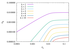
Figure 11: Concentration of loops made of $k$ strands as a function of $c_{\text{t}}$ for $K=10^{4}$ and $c_{\text{i}}=10^{-2}$ for case 1.

Recent literature provides a plethora of examples for supramolecular self-assembly where more than two compounds or types of bonds are involved. Winter and Schubert, for instance, distinguish six different classes of supramolecular polymerization only regarding metallo-supramolecular polymers, see Figure 3 of Ref. (Winter and Schubert, 2016). Here class Ia) is equivalent to case 1, Ib) and IIa) are case 3 in our notation, and Ic is case 2a. Molecular weight distributions for more complex classes like IIb) and IIc) of Ref. (Winter and Schubert, 2016) can be derived using our results. For instance, class IIc) is equivalent to case 3 after considering that loop formation is enhanced by a factor of two similar to case 2a, while class IIb) requires the consideration of quadruples of units with two instead of one stoichiometric ratio. Thus, class IIb) is also a generalization of case 3. Our theoretical analysis may serve as a template to derive weight distributions for these and other more complex cases.

In the sections above, we have discussed only LGS which refers to polymer melts or $\theta$-solutions. A generalization to good or a-thermal solvent is discussed in Ref. (Lang and Kumar, 2021) along with a discussion of poor solvents that applies also to case 2b where all macromonomers are of the same type. Case three in the presence of a poor and probably selective solvent with reactions occurring across a phase boundary is a quite complex problem that goes clearly beyond the scope of the present paper. We postpone the discussion of this subject to forthcoming work.

A generalization with respect to a first shell substitution effect is straight forward, since this effect requires to consider different reaction constants in the two balance equations that connect either $\text{w}_{1}$ with $\text{w}_{0}$ and $\text{w}_{1}$ with $\text{w}_{2}.$ Similarly, the balance equations of loops need to be modified, if loop closure occurs starting from a chain end on $\text{w}_{1}$ or on $\text{w}_{2}$. More details on the implementation of a first shell substitution effect can be found in our preceding work (Lang and Kumar, 2021).

Our approach provides molecular weight distributions for linear chains and rings in theta solvents (good solvents require some adjustments discussed in Ref. (Lang and Kumar, 2021) and could be computed numerically). These can be incorporated in models for the properties of the corresponding supramolecular solutions that do consider polydispersity. We expect that such a generalization provides a more accurate analsis of experimental data of supramolecular solutions.

V Summary

In the present work, we have developed an exact numerical solution for the stepwise reversible alternating co-polymerization of two strands of type $A$ and $B$ and the stepwise reversible polymerization of linear precursors where both ends participate in two orthogonal reactions. Both systems were treated exactly in the mean field limit for both cases with and without cyclization. Our discussion shows that the system with the orthogonal reactions is particularly suited to suppress cyclization in contrast to a reaction of the same chain architecture where the ends undergo a hetero-complementary coupling of $A$ with $B$ reactive groups. This latter system leads to largest weight fractions of cyclics at otherwise identical parameters like intra- and inter-molecular concentrations of reactive groups and an identical reaction constant.

All four systems that we have studied develop a comparatively large polydispersity (see also Ref. (Lang and Kumar, 2021) regarding case 1 and case 2a at concentrations about four to ten times larger than the intra-molecular concentration. The critical concentration is not universal, it appears at different ratios of the inter- to the intra-molecular concentration of the reactive groups depending on the particular reaction mechanism. One important point of the discussion is that cyclic species are always at 100% conversion and are always stoichiometrically balanced in case of an alternating co-polymerization. Therefore, any deviation from stoichiometry or complete reactions is compensated by the remaining linear species alone. This causes a systematic split of the properties of the linear and cyclic chain fractions and shows a strong impact on the corresponding distributions and averages.

We have tested our theory by comparing with Monte Carlo simulations that were developed in Ref. (Lang and Kumar, 2021). These simulations resemble the mean field limit by employing a set of Gaussian strands that react only according to given concentrations and reaction constants. The observed excellent agreement with the simulation data, therefore, is a strong support for our analytical discussion. We expect that our work will be applied to develop theory for more complex supramolecular systems and regarding a more accuarate analysis of experimental data.

VI Acknowledgements

The authors thank the ZIH Dresden for a generous grant of computation time and the DFG for funding Project LA2735/5-1. The authors also thank Frank Böhme, Reinhard Scholz, and Toni Müller for useful comments on earlier versions of the manuscript.

VII Appendix

VII.1 Case 3 without rings

As mentioned in the main part of this work, we compute number and weight distributions of all classes of chains, specific averages and total average degrees of polymerization, since previous work contains some obvious mistakes (wrong normalization (Flory, 1936), non-integer powers of some probabilities (Mizerovskii and Padokhin, 2013), etc.). Furthermore, not all required distributions and averages were computed before. This gap is closed with the derivation below.

We consider a case 3 polymerization where LGS with functional groups of type $A$ react exclusively with functional groups of type $B$ that are located on a second fraction of LGS. The molar ratio of type $A$ strands to type $B$ strands is defined as the stoichiometric ratio $r$, see equation (1). For simplification, we assume that both strands have roughly the same molar mass, which allows a simplified treatment based upon degrees of polymerization that we define with respect to the number of precursor strands in one molecule. As notation, we use $p_{\text{A}}=p$ for the conversion of the minority $A$ groups, $c_{\text{A}}$ and $c_{\text{B}}$ for the concentration of $A$ and $B$ groups respectively, and $c_{\text{o,A}}$ and $c_{\text{o,B}}$ as the concentration of the non-paired $A$ and $B$ groups respectively.

We introduce the total concentration of reactive groups, $c_{\text{t}}$, as the sum of the total concentrations of $A$ and $B$ groups, see equation (2). Since total conversion is defined with respect to the maximum possible conversion, there is

$$p=p_{\text{A}}=1-\frac{c_{\text{o,A}}}{c_{\text{A}}}$$ (A1)

and the conversion of the $B$ groups is

$$p_{\text{B}}=rp=1-\frac{c_{\text{o,B}}}{c_{\text{B}}}.$$ (A2)

The concentration of the reaction products is the concentration of the reacted minority $A$ groups, $c_{\text{A}}-c_{\text{o,A}},$ since there is one reacted $A$ group per bond. Note that this concentration equals the concentration of the reacted $B$ groups,

$$c_{\text{B}}-c_{\text{o,B}}=c_{\text{A}}-c_{\text{o,A}}$$ (A3)

and that the concentration of the open $A$ groups can be expressed in terms of concentrations of the $B$ groups

$$c_{\text{o,A}}=c_{\text{o,B}}-c_{\text{B}}+c_{\text{A}}=c_{\text{o,B}}+c_{\text{B}}\left(r-1\right).$$ (A4)

The total concentration of reactive groups is

$$c_{\text{A}}+c_{\text{B}}=\left(r+1\right)c_{\text{B}}.$$ (A5)

Thus, the product of the concentration of the reactants is

$$c_{\text{o,A}}c_{\text{o,B}}=c_{\text{o,B}}\left(c_{\text{o,B}}+c_{\text{B}}\left(r-1\right)\right)$$ (A6)

This leads to a law of mass action with reaction constant

$$K=\frac{c_{\text{B}}-c_{\text{o,B}}}{c_{\text{o,B}}\left(c_{\text{o,B}}+c_{\text{B}}\left(r-1\right)\right)}.$$ (A7)

Note that there is exactly one $A$ and $B$ group per bond, thus, there is no factor of two in the definition of $K$ in contrast to case 1, see Ref. (Lang and Kumar, 2021). This last equation can be solved for $c_{\text{o,B}}$, which provides

$$c_{\text{o,B}}=$$ (A8)

$$\frac{\left(c_{\text{B}}^{2}K^{2}\left(r-1\right)^{2}+2c_{\text{B}}K(r+1)+1\right)^{1/2}+c_{\text{B}}K(1-r)-1}{2K}$$

and conversion of $B$ groups through

$$p_{\text{B}}=1-\frac{c_{\text{o,B}}}{c_{\text{B}}}$$ (A9)

Finally, $p$ is given by $p_{\text{B}}/r$, see equation (A2).

This solution is tested with simulation data in Figure 12, and excellent agreement is found. Note that the above solution does not converge towards equation (4) of Ref. (Lang and Kumar, 2021) for the same total concentration of reactive groups, since $c_{\text{A}}=c_{\text{B}}$ for $r=1$. In fact, the case $r=1$ is equivalent to the homopolymerization of $A-B$ monomers (case 2a) where $A$ groups react exclusively with $B$ groups. Note that $p_{\text{A}}$ is significantly below one for a broad range $Kc_{\text{B}}$. Therefore, the 100% case discussed in Ref. (Jacobson and Stockmayer, 1950) with $p_{\text{A}}=1$ serves as an approximation only in the limit of large $Kc_{\text{B}}$.

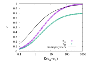
Figure 12: $p_{\text{A}}$ and $p_{\text{B}}$ as a function of $\left(c_{\text{A}}+c_{\text{B}}\right)K$ for a stoichiometric $r=0.8$ in the absence of loop formation, $c_{\text{i}}=0$ (case 3). The thick black line refers to reversible homopolymers with identical end groups on both chain ends, equation (4) of Ref. (Lang and Kumar, 2021).

In the reaction product, we classify the resulting molecules whether these are terminated by only $A$ groups, only $B$ groups or both (mixed “$m$” terminated). The weight fractions of these different types of chains will be denoted below by $\text{w}_{\text{A}}$, $\text{w}_{\text{B}}$, and $\text{w}_{\text{m}}$ respectively, while the number fractions are denoted by $n_{\text{A}}$, $n_{\text{B}}$, and $n_{\text{m}}$. For the computation of the molecular weight fractions, we start with the total density of chain ends that is given by the total concentration of non-paired (“open”) reactive groups

$$c_{\text{o}}=c_{\text{A}}\left(1-p\right)+c_{\text{B}}\left(1-rp\right)=\left(1+r-2rp\right)c_{\text{B}}.$$ (A10)

The ratio between the concentration of all reactive groups and $c_{\text{o}}$ provides the average DP

$$N_{\text{n}}=\frac{c_{\text{A}}+c_{\text{B}}}{c_{\text{o}}}=\frac{1+r}{1+r-2rp}.$$ (A11)

For a simple derivation of the number fraction distributions, let us introduce an unknown normalization constant $Y$ to be determined later. The probability that a chain end of type $A$ is selected randomly as a starting point of a chain, $P_{\text{end}}\left(A\right)$ is equal to the portion of non-reacted $A$ groups among all non-reacted chain ends,

$$P_{\text{end}}\left(A\right)=\frac{c_{\text{A}}\left(1-p\right)}{c_{\text{o}}}=\frac{r(1-p)}{1+r-2rp}.$$ (A12)

Furthermore, a portion of $(1-p)$ of all $A$ groups terminates a chain. Thus, we expect a dependence for the number fraction of all $A$ terminated chains like

$$n_{\text{A}}=P_{\text{end}}\left(A\right)(1-p)X=\frac{r\left(1-p\right)^{2}}{1+r-2rp}Y.$$ (A13)

Similarly, $B$ strands are selected as starting points of a chain with a probability $1-P_{\text{end}}\left(A\right)$ among all chain ends, while also a portion of $1-rp$ strands terminates a chain. Thus,

$$n_{\text{B}}=\left(1-P_{\text{end}}\left(A\right)\right)(1-rp)Y=\frac{\left(1-rp\right)^{2}}{1+r-2rp}Y.$$ (A14)

Finally, mixed terminated chains start from an AB pair of strands. This pair requires a bond in between that exists with probability $rp$ (when starting from a $B$ end with probability $1-P_{\text{end}}\left(A\right)$ and terminating at an $A$ with termination probability $1-p$) or with probability $p$ (when starting from an $A$ end with probability $P_{\text{end}}\left(A\right)$ and terminating at a $B$ with termination probability $1-rp$). Together these two cases provide

$$n_{\text{m}}=\frac{2rp(1-p)(1-rp)}{1+r-2rp}Y.$$ (A15)

The $Y$ in the above three cases is a normalization factor that accounts for the weight distribution of strands. This normalization factor is conveniently computed from the normalization of the number fractions

$$n_{\text{m}}+n_{\text{A}}+n_{\text{B}}=1.$$ (A16)

This provides

$$Y^{-1}=\frac{\left(1-p\right)^{2}r+\left(1-rp\right)^{2}+2rp(1-p)(1-rp)}{\left(r(1-p)+1-rp\right)}$$

$$=1-rp^{2}$$ (A17)

for $n_{\text{A}}$, $n_{\text{B}}$, and $n_{\text{m}}$. To understand the physical origin of $Y$ let us introduce the probability $q=rp^{2}$ that an $AB$ strand pair is added to an existing chain. What we have left out in our derivation above is the distribution of additional pairs of $A$ and $B$ strands that are attached to a given set of chain ends. The probability of finding chain ends with $z$ added $AB$ pairs decays as $q^{z}.$ Since

$$\sum_{z=0}^{\infty}q^{z}=\frac{1}{1-q}=\frac{1}{1-rp^{2}}=Y,$$ (A18)

we see indeed that the normalization factor is the sum over the number fraction distribution of chains (with the same ends). Note that with the last two equations we also have demonstrated that the number fraction distributions are properly normalized.

Putting together the above relations, we can write down the number fraction distributions of all chains depending on end groups and the number $z\geq 0$ of additional pairs $AB$ of strands,

$$n_{\text{m,z}}=p^{2z}r^{z}\frac{2rp\left(1-p\right)\left(1-rp\right)}{1+r-2rp}$$ (A19)

$$n_{\text{A,z}}=p^{2z}r^{z}\frac{r\left(1-p\right)^{2}}{1+r-2rp}$$ (A20)

$$n_{\text{B,z}}=p^{2z}r^{z}\frac{\left(1-rp\right)^{2}}{1+r-2rp}.$$ (A21)

The shortest realizations of an $A$, $B$, or $m$-terminated chain ($z=0$) are a single $A$ or $B$ strand or a single $AB$ dimer respectively. Note that the distributions, equation (A19) to equation (A21), agree with older work (e.g. equation (20), (29), and (30) of Ref. (Flory, 1936)). More recent work arrives at different results (e.g. the fourth equation from the bottom on page 344 of Ref. (Mizerovskii and Padokhin, 2013)).

For simplicity, let us assume that the molar mass of an $A$ strand equals the molar mass of a $B$ strand. The weight fractions of $A$, $B$, or $m$ terminated chains are then obtained in the standard way by multiplying the corresponding number fraction distribution with the number of strands over $N_{\text{n}}$. For $X=A,B,m$ we write this as

$$\text{w}_{\text{X,z}}=\frac{y_{X}(z)}{N_{\text{n}}}n_{\text{X,z}}$$ (A22)

where we use a function

$$y_{\text{m}}(z)=2\left(z+1\right),$$ (A23)

for mixed terminated chains that becomes

$$y_{\text{X}}(z)=2z+1$$ (A24)

for $X=A,B$. This function counts the number of strands in a chain with $z$ additional pairs of strands beyond the smallest chain in this class.

We obtain

$$\text{w}_{\text{m,z}}=2\left(z+1\right)p^{2z}r^{z}\left[\frac{2pr\left(1-p\right)\left(1-rp\right)}{1+r}\right]$$ (A25)

$$\text{w}_{\text{A,z}}=\left(2z+1\right)p^{2z}r^{z}\left[\frac{r\left(1-p\right)^{2}}{1+r}\right]$$ (A26)

$$\text{w}_{\text{B,z}}=\left(2z+1\right)p^{2z}r^{z}\left[\frac{\left(1-rp\right)^{2}}{1+r}\right].$$ (A27)

Note that these equations agree with Flory’s work except for $w_{\text{A,z}}$ that contains one extra power in $r$ in comparison with equation (27) of Ref. (Flory, 1936). Most likely, this was just a misprint, since Flory provides correct number fractions that were derived from the incorrect equation (27). Note that Ref. (Mizerovskii and Padokhin, 2013) agrees with Flory regarding all $w_{\text{X}}$ and does not recognize this mistake.

To simplify notation, let us denote the terms in the square brackets of equation (A25) to (A27) by $E_{\text{m}}$, $E_{\text{A}}$, and $E_{\text{B}}$ respectively. We further set $q=rp^{2}$ and use the moments

$$m_{1}\left(2z+2\right)=\sum_{z=0}^{\infty}\left(2z+2\right)q^{z}=\frac{2}{\left(1-q\right)^{2}}$$ (A28)

$$m_{1}(2z+1)=\sum_{z=0}^{\infty}\left(2z+1\right)q^{z}=\frac{1+q}{\left(1-q\right)^{2}}$$ (A29)

$$m_{2}\left(2z+2\right)=\sum_{z=0}^{\infty}\left(2z+2\right)^{2}q^{z}=4\frac{1+q}{\left(1-q\right)^{3}}$$ (A30)

$$m_{2}(2z+1)=\sum_{z=0}^{\infty}\left(2z+1\right)^{2}q^{z}=\frac{1+6q-q^{2}}{\left(1-q\right)^{3}}.$$ (A31)

The total weight fraction of each termination class is then

$$\text{w}_{\text{m}}=m_{1}\left(2z+2\right)E_{\text{m}}$$ (A32)

and for $X=A,B$ there is

$$\text{w}_{\text{X}}=m_{1}(2z+1)E_{\text{X}}$$ (A33)

As a test, we have checked normalization by computing $\text{w}_{\text{m}}+\text{w}_{\text{A}}+\text{w}_{\text{B}}$, which is indeed unity for our set of equations but not for the equations provided in Refs. (Flory, 1936; Mizerovskii and Padokhin, 2013). Therefore, dependent results like weight average DP or polydispersity in these works need to be questioned.

The weight average DP is computed as $m_{2}/m_{1}$ where the $E_{\text{X}}$ terms for all $X=A,$ $B$, and $m$ cancel out. This yields

$$N_{\text{w,m}}=\frac{m_{2}\left(2z+2\right)}{m_{1}\left(2z+2\right)}=2\left(\frac{1+q}{1-q}\right)$$ (A34)

$$N_{\text{w,A}}=N_{\text{w,B}}=\frac{m_{2}\left(2z+1\right)}{m_{1}\left(2z+1\right)}=\frac{1+6q+q^{2}}{1-q^{2}}$$ (A35)

The last two equations allow to compute the total weight average DP through

$$N_{\text{w}}=N_{\text{w,m}}\text{w}_{\text{m}}+N_{\text{w,A}}\left(1-\text{w}_{\text{m}}\right).$$ (A36)

Here the $E_{\text{X}}$ terms do not cancel, and a rather complex result is obtained that we do not reproduce here. The number average DP of the mixed terminated chains is given by

$$N_{\text{n,m}}=\frac{2\sum_{z=0}^{\infty}\left(z+1\right)q^{z}}{\sum_{z=0}^{\infty}q^{z}}=\frac{2}{1-q}$$ (A37)

while the number average DP of the $A$ and $B$ terminated chains is less by one,

$$N_{\text{n,A}}=N_{\text{n,m}}-1=\frac{1+q}{1-q}=N_{\text{n,B}},$$ (A38)

since the weight distribution starts from a single strand and not from a pair. Finally, the polydispersities are

$$\frac{N_{\text{w,m}}}{N_{\text{n,m}}}=1+q$$ (A39)

$$\frac{N_{\text{w,A}}}{N_{\text{n,A}}}=\frac{N_{\text{w,B}}}{N_{\text{n,B}}}=\frac{1+6q+q^{2}}{\left(1+q\right)^{2}}.$$ (A40)

Note that the first of these polydispersities is equivalent to the polydispersity of a most probable distribution for $r=1$. The second result is identical to the polydispersity of an alternating co-polymerization at full conversion (Lang and Böhme, 2019), which supports that also the averages for the $A$ and $B$ terminated chains and all intermediate steps are correct. Note that Flory (Flory, 1936) did not compute weight averages and polydispersity, while Mizerovskii and Padokhin (Mizerovskii and Padokhin, 2013) arrive at several expressions that contain non-integer powers of probabilities like $r$. Such results are obviously not correct, since the probability $r$ is associated with the existence of $A$ strands: these either exist or not, but they cannot adopt any state in between.

VII.2 Case 2b without rings

We consider the polymerization of linear strands with two different reactive groups $A$ and $B$ on either end forming exclusively $AA$ and $BB$ bonds with a probability $p_{\text{A}}$ and $p_{\text{B}}$, respectively. To compute these conversions, we assume the independence of the reactions of $A$ and $B$ groups. In the absence of intra-molecular reactions, these establish separate equilibrium concentrations of closed stickers according to (Stukhalin et al., 2013; Lang and Kumar, 2021)

$$p_{\text{X}}=1-\frac{\left(1+8K_{\text{X}}c_{\text{X}}\right)^{1/2}-1}{4K_{\text{X}}c_{\text{X}}}$$ (A41)

where $K_{\text{X}}$ is the reaction constant for $X=A,B$ groups respectively, and $c_{\text{X}}=c_{\text{A}}=c_{\text{B}}$. Note that here a factor of $2K$ appears instead of $K$ as in case 1, since the concentration of $B$ groups does not play any role for reactions of $A$ groups and vice versa, see also the discussion around equation (2) of Ref. (Lang and Kumar, 2021). Total conversion is given by

$$p=\left(p_{\text{A}}+p_{\text{B}}\right)/2.$$ (A42)

The derivation below follows closely the steps in the preceding section concerning case 3. Therefore, we skip here most of the discussion, except for deviations from case 3.

When picking randomly a chain end, a fraction of

$$P_{\text{end}}\left(A\right)=\left(1-p_{\text{A}}\right)/\left(2-p_{\text{A}}-p_{\text{B}}\right)$$ (A43)

of these ends is of type $A$, while a fraction of $1-P_{\text{end}}\left(A\right)$ is of type $B$. The average degree of polymerization of the linear chains, $N_{\text{n}}$, is the concentration of reactive groups divided by the concentration of chain ends

$$N_{\text{n}}=\frac{2c_{\text{A}}}{c_{\text{A}}\left(2-p_{\text{A}}-p_{\text{B}}\right)}=\frac{1}{1-p}.$$ (A44)

In analogy to the derivation in the preceding section Case 3 without rings, we set $q=p_{\text{A}}p_{\text{B}}$ with $\sum_{z=0}^{\infty}q^{z}=\left(1-q\right)^{-1}$. $z$ counts again the number of additional pairs of strands beyond the shortest possible chain of a particular group. In contrast to the preceding section, the $A$- and $B$-terminated chains consist now of an even number of strands, while the $m$ terminated chains contain an odd number of strands. Thus, the arguments previously used for the mixed terminated chains provide

$$n_{\text{A}}=P_{\text{end}}\left(A\right)p_{\text{B}}\left(1-p_{\text{A}}\right)\sum_{z=0}^{\infty}q^{z}$$ (A45)

$$=\frac{p_{\text{B}}\left(1-p_{\text{A}}\right)^{2}}{\left(2-p_{\text{A}}-p_{\text{B}}\right)\left(1-p_{\text{A}}p_{\text{B}}\right)},$$

$$n_{\text{B}}=\frac{p_{\text{A}}\left(1-p_{\text{B}}\right)^{2}}{\left(2-p_{\text{A}}-p_{\text{B}}\right)\left(1-p_{\text{A}}p_{\text{B}}\right)},$$ (A46)

while, conversely, we find

$$n_{\text{m}}=\frac{2\left(1-p_{\text{A}}\right)\left(1-p_{\text{B}}\right)}{\left(2-p_{\text{A}}-p_{\text{B}}\right)\left(1-p_{\text{A}}p_{\text{B}}\right)}.$$ (A47)

We obtain for the number fraction distributions

$$n_{\text{A,z}}=p_{\text{A}}^{z-1}p_{\text{B}}^{z}\frac{\left(1-p_{\text{A}}\right)^{2}}{\left(2-p_{\text{A}}-p_{\text{B}}\right)},$$ (A48)

$$n_{\text{B,z}}=p_{\text{B}}^{z-1}p_{\text{A}}^{z}\frac{\left(1-p_{\text{B}}\right)^{2}}{\left(2-p_{\text{A}}-p_{\text{B}}\right)},$$ (A49)

and

$$n_{\text{m,z}}=\left(p_{\text{A}}p_{\text{B}}\right)^{z-1}\frac{2\left(1-p_{\text{A}}\right)\left(1-p_{\text{B}}\right)}{\left(2-p_{\text{A}}-p_{\text{B}}\right)}.$$ (A50)

Let us again use $q=p_{\text{A}}p_{\text{B}}$ to simplify the notation for the higher moments of the distribution. With an adapted version of equation (A22) where even and odd terms are mutually exchanged for $m\rightleftharpoons A,B$, we obtain for the weight fraction distributions that these correspond to

$$\text{w}_{\text{A,z}}=\left(2z+2\right)q^{z-1}\left[p_{\text{B}}\left(1-p_{\text{A}}\right)^{2}/2\right],$$ (A51)

$$\text{w}_{\text{B,z}}=\left(2z+2\right)q^{z-1}\left[p_{\text{A}}\left(1-p_{\text{B}}\right)^{2}/2\right],$$ (A52)

and

$$\text{w}_{\text{m,z}}=\left(2z+1\right)q^{z-1}\left[\left(1-p_{\text{A}}\right)\left(1-p_{\text{B}}\right)\right].$$ (A53)

The terms in the square brackets are denoted below by $E_{\text{X}}$ with $X=A,B,m$ accordingly. These do not change for higher order averages. We further use the moments defined in equation (A28) to (A31). The weight fractions of chains in each termination class are then

$$\text{$\text{w}_{\text{A}}=$}m_{1}\left(2z+2\right)E_{\text{A}},$$ (A54)

$$\text{$\text{w}_{\text{B}}=$}m_{1}\left(2z+2\right)E_{\text{B}},$$ (A55)

and

$$\text{$\text{w}_{\text{m}}=$}m_{1}\left(2z+1\right)E_{\text{m}}.$$ (A56)

As above, the weight average degrees of polymerization are obtained by the ratio of the moments $m_{\text{2}}/m_{1}$ of the corresponding even and odd terms. This yields

$$N_{\text{w},\text{A}}=2\frac{1+q}{1-q}=N_{\text{w,B}}$$ (A57)

and

$$N_{\text{w,m}}=\frac{1+6q+q^{2}}{1-q^{2}}$$ (A58)

with a weight average DP in the full sample of

$$N_{\text{w}}=N_{\text{w,m}}\text{w}_{\text{m}}+N_{\text{w,A}}\left(1-\text{w}_{\text{m}}\right).$$ (A59)

The number average degrees of polymerization are

$$N_{\text{n,A}}=\frac{2\sum_{z=0}^{\infty}\left(z+1\right)q^{z}}{\sum_{z=0}^{\infty}q^{z}}=\frac{2}{1-q}=N_{\text{n,B}}$$ (A60)

$$N_{\text{n,m}}=N_{\text{n,A}}-1=\frac{1+q}{1-q}$$ (A61)

and polydispersities are

$$\frac{N_{\text{w,A}}}{N_{\text{n,A}}}=\frac{N_{\text{w,B}}}{N_{\text{n,B}}}=1+q$$ (A62)

$$\frac{N_{\text{w,m}}}{N_{\text{n,m}}}=\frac{1+6q+q^{2}}{\left(1+q\right)^{2}}.$$ (A63)

Altogether, the higher moments of the distributions are equivalent to case 3. However, the $A$- and $B$- terminated chains contain now an even number of strands and have the corresponding higher order averages, while the $m$-terminated chains contain an odd number of strands with the corresponding higher order averages.

References

- McBride et al. (2019) McBride, M. K.; Worrell, B. T.; Brown, T.; Cox, L. M.; Sowan, N.; Wang, C.; Podgorski, M.; Martinez, A. M.; Bowman, C. N. Annu. Rev. Chem. Biomol. Eng. 2019, 10, 175–198.
- Campanella et al. (2018) Campanella, A.; Döhler, D.; Binder, W. H. Macromol. Rapid. Commun. 2018, 39, 1700739.
- Hodge (2015) Hodge, P. Polym. Adv. Technol. 2015, 26, 797–803.
- Bapat et al. (2020) Bapat, A. P.; Sumerlin, B. S.; Sutti, A. Materials Horizons 2020, 7, 694–714.
- Zhang et al. (2018) Zhang, Z. P.; Rong, M. Z.; Zhang, M. Q. Prog. Polym. Sci. 2018, 80, 39–93.
- Flory (1953) Flory, P. J. Principles of polymer chemistry; Cornell University Press, 1953.
- Kapnistos et al. (2008) Kapnistos, M.; Lang, M.; Vlassopoulos, D.; Pyckhout-Hintzen, W.; Richter, D.; Cho, D.; Chang, T.; Rubinstein, M. Nature Materials 2008, 7, 997–1002.
- Michieletto and Turner (2016) Michieletto, D.; Turner, M. S. PNAS 2016, 113, 5195–5200.
- Grosberg et al. (1996) Grosberg, A. Y.; Feigel, A.; Rabin, Y. Phys. Rev. E 1996, 54, 6618–6622.
- Lang et al. (2012) Lang, M.; Fischer, J.; Sommer, J.-U. Macromolecules 2012, 45, 7642–7648.
- Zhou et al. (2019) Zhou, Y.; Hsiao, K.-W.; Regan, K. E.; Kong, D.; McKenna, G. B.; Robertson-Anderson, R. M.; Schroeder, C. M. Nature Commun. 2019, 10, 1753.
- Lang et al. (2015) Lang, M.; Rubinstein, M.; Sommer, J.-U. ACS Macro Letters 2015, 4, 177–181.
- Lang (2013) Lang, M. Macromolecules 2013, 46, 1158–1166.
- Lang and Kumar (2021) Lang, M.; Kumar, K. S. Macromolecules 2021, 54, in press.
- Jacobson and Stockmayer (1950) Jacobson, H.; Stockmayer, W. H. J. Chem. Phys. 1950, 18, 1600–1606.
- Flory (1936) Flory, P. J. J. Am. Chem. Soc. 1936, 58, 1877–1885.
- Bras et al. (2013) Bras, A. R.; Hövelmann, C. H.; Antonius, W.; Teixeira, J.; Radulescu, A.; Allgaier, J.; Pyckhout-Hintzen, W.; Wischnewski, A.; Richter, D. Macromolecules 2013, 46, 9446–9454.
- Mansfeld et al. (2013) Mansfeld, U.; Winter, A.; Hager, M. D.; Günther, W.; Altunas, E.; Schubert, U. S. J. Pol. Sci. A 2013, 51, 2006–2015.
- Hofmeier and Schubert (2005) Hofmeier, H.; Schubert, U. S. Chem. Commun. 2005, 2423–2432.
- Gröger et al. (2011) Gröger, G.; Meyer-Zaika, W.; Böttcher, C.; Gröhn, F.; Ruthard, C.; Schmuck, C. J. Am. Chem. Soc. 2011, 133, 8961–8971.
- Li et al. (2012) Li, S.-T.; Xiao, T.; Lin, C.; Wang, L. Chem. Soc. Revs. 2012, 41, 5950–5968.
- Qian et al. (2016) Qian, X.; Gong, W.; Li, X.; Fang, L.; Kuang, X.; Ning, G. Chem. Eur. J 2016, 22, 6881–6890.
- Sataux et al. (2018) Sataux, J.; de Espinosa, L. M.; Balog, S.; Weder, C. Macromolecules 2018, 51, 5867–5874.
- Gu et al. (2015) Gu, R.; Yao, F.; Fu, X.; Zhou, Q.; Qu, D.-H. Chem. Commun. 2015, 51, 5429–5431.
- Moratti (2005) Moratti, S. C. Macromolecules 2005, 38, 1520–1522.
- Gentekos et al. (2019) Gentekos, D. T.; Sifri, R. J.; Fors, B. P. Nature Revs. Materials 2019, 4, 761–774.
- Mizerovskii and Padokhin (2013) Mizerovskii, L. N.; Padokhin, V. A. Fibre Chem. 2013, 44, 337–355.
- Szymanski (1989) Szymanski, R. Makromol. Chem. 1989, 190, 2903–2908.
- Szymanski (1992) Szymanski, R. Prog. Polym. Sci. 1992, 17, 917–951.
- Vermonden et al. (2003) Vermonden, T.; van der Gucht, J.; de Waard, P.; Marcelis, A. T. M.; Besseling, N. A. M.; Sudhölter, E. J. R.; Fleer, G. J.; Cohen Stuart, M. A. Macromolecules 2003, 36, 7035–7044.
- Suckow et al. (2019) Suckow, M.; Lang, M.; Komber, H.; Pospiech, D.; Wagner, M.; Weinelt, F.; Baumann, F.-E.; Böhme, F. Polym. Chem. 2019, 10, 1930–1937.
- Stockmayer (1944) Stockmayer, W. H. J. Chem. Phys. 1944, 12, 125–131.
- Flory (1946) Flory, P. J. Chemistry Reviews 1946, 39, 137–197.
- Macosko and Miller (1976) Macosko, C. W.; Miller, D. R. Macromolecules 1976, 9, 199–206.
- Stukhalin et al. (2013) Stukhalin, E. B.; Cai, L.-H.; Kumar, N. A.; Leibler, L.; Rubinstein, M. Macromolecules 2013, 46, 7525–7541.
- Ovchinnikov and Zeldovich (1978) Ovchinnikov, A. A.; Zeldovich, Y. B. Chemical Physics 1978, 28, 215–218.
- Toussaint and Wilczek (1983) Toussaint, D.; Wilczek, F. J. Chem. Phys. 1983, 78, 2642–2647.
- Kang and Redner (1984) Kang, K.; Redner, S. Phys. Rev. Lett. 1984, 52, 955–958.
- Rey and Cardy (1999) Rey, P.-A.; Cardy, J. J. Phys. A 1999, 32, 1585–1603.
- Gopich et al. (2001) Gopich, I. V.; Ovchinnikov, A. A.; Szabo, A. Phys. Rev. Lett. 2001, 86, 922–925.
- Ercolani et al. (1993) Ercolani, G.; Mandolini, L.; Mencarelli, P.; Roelens, S. J. Am. Chem. Soc. 1993, 115, 3901–3908.
- Di Stefano and Mandolini (2019) Di Stefano, S.; Mandolini, L. Phys. Chem. Chem. Phys. 2019, 21, 955–987.
- Winter and Schubert (2016) Winter, A.; Schubert, U. S. Chem. Soc. Rev. 2016, 45, 5311–5357.
- Lang and Böhme (2019) Lang, M.; Böhme, F. Macromol. Theory Simul. 2019, 1800069.