The appearance of a merging binary black hole very close to a spinning supermassive black hole

Abstract

The mass and distance of a binary black hole (BBH) are fundamental parameters to measure in gravitational-wave (GW) astronomy. It is well-known that the measurement is affected by cosmological redshift, and recent works also showed that Doppler and gravitational redshifts could further affect the result if the BBH coalesces close to a supermassive black hole (SMBH). Here we consider the additional lensing effect induced by the nearby SMBH on the measurement. We compute the null geodesics originating within $10$ gravitational radii of a Kerr SMBH to determine the redshift and magnification of the GWs emitted by the BBH. We find a positive correlation between redshift and demagnification, which results in a positive correlation between the mass and distance of the BBH in the detector frame. More importantly, we find a higher probability for the signal to appear redshifted and demagnified to a distant observer, rather than blueshifted and magnified. Based on these results, we show that a binary at a cosmological redshift of $z_{\rm cos}=(10^{-2}-10^{-1})$ and composed of BHs of $(10-20)M_{\odot}$ could masquerade as a BBH at a redshift of $z_{\rm cos}\sim 1$ and containing BHs as large as $(44-110)M_{\odot}$. In the case of extreme demagnification, we also find that the same BBH could appear to be at $z_{\rm cos}>10$ and contain subsolar-mass BHs. Such an effect, if not accounted for, could bias our understanding of the origin of the BHs detected via GWs.

1 Introduction

The majority of the black holes (BHs) detected by the Laser Interferometer Gravitational-wave Observatory (LIGO) and the Virgo detectors (The LIGO Scientific Collaboration et al., 2021b) are several times more massive than those BHs found previously in X-ray binaries (McClintock et al., 2014; Corral-Santana et al., 2016). The discrepancy raises an interesting question about the formation channel of the LIGO/Virgo binary BHs (BBHs). Conventional models suggest that massive BBHs could form as a result of the evolution of isolated binary massive stars or the dynamical interactions between the BHs in star clusters (see LIGO Scientific Collaboration & Virgo Collaboration, 2016; The LIGO Scientific Collaboration & The Virgo Collaboration, 2019; LIGO Scientific Collaboration & Virgo Collaboration, 2020, for summaries).

Another place where the LIGO/Virgo massive BBHs could form is the vicinity of a supermassive black hole (SMBH, $10^{6}-10^{10}M_{\odot}$). First, massive objects such as BHs could accumulate here due to a dynamical process called “mass segregation” (O’Leary et al., 2009). It is also difficult for BHs to leave the system because of the large escape velocity induced by the SMBH (Miller & Lauburg, 2009). Second, by interacting with the SMBH (Antonini & Perets, 2012) or the other massive compact objects trapped in the galactic nucleus (Leigh et al., 2018; Yang et al., 2019), a BBH could more effectively merge. Third, if the SMBH is surround by a gaseous disk, as would be the case in an active galactic nucleus (AGN), BBHs could form and merge even more efficiently by interacting with the gas (e.g. Baruteau et al., 2011; McKernan et al., 2012; Bartos et al., 2017; Stone et al., 2017). According to the estimations in the literature, the merger rate of the BBHs in galactic nuclei is comparable to the rate inferred from the BBHs detected by LIGO/Virgo (Fragione et al., 2019; Tagawa et al., 2019; Arca Sedda, 2020; Gröbner et al., 2020; Ford & McKernan, 2021; The LIGO Scientific Collaboration & The Virgo Collaboration, 2021; Zhang et al., 2021; Samsing et al., 2022).

More recent studies have shown that about $(1-2)\%$ of the LIGO/Virgo BBHs could come from a distance smaller than $10$ Schwarzschild radii from a SMBH (Chen & Han, 2018; Addison et al., 2019; Peng & Chen, 2021). The distance could be as small as $2-3$ gravitational radii if the central SMBH is rapidly spinning (Chen & Zhang, 2022). Although such binaries constitute only a small fraction of the BBH population, the fact that LIGO/Virgo have so far detected $\sim 90$ BBHs (The LIGO Scientific Collaboration et al., 2021c) indicates that one or two of them may have come from the vicinity of a SMBH.

Interestingly, a BBH so close to a SMBH could appear significantly more massive than it really is (Chen et al., 2019). This effect is analogous to the famous “mass-redshift degeneracy” (Schutz, 1986) but now the redshift is caused not only by the expansion of the universe, but also the gravitational and Doppler redshifts induced by the SMBH. The additional redshifts effectively lower the observed frequency ($f$) and chirp rate ($\dot{f}$) of a gravitational-wave (GW) signal. Since $f$ and $\dot{f}$ are used to infer the mass of a BBH in the standard procedure of GW data analysis, the inferred mass could be significantly larger than the intrinsic mass if an observer, unaware of the presence of the SMBH, neglects the effects induced by the gravitational and Doppler redshifts (Chen, 2021).

Identifying these fake massive BBHs close to SMBHs is particularly important given the current ambiguity of the origin of the LIGO/Virgo sources. It is also very challenging because the signal normally lasts less than a second in the LIGO/Virgo band. The short duration of the signals, in contrast to the long orbital period (tens to thousands of seconds) of the BBH around the SMBH, makes it difficult to discern any signature caused by the acceleration of the GW source around the SMBH (e.g. Bonvin et al., 2017; Inayoshi et al., 2017; Meiron et al., 2017).

It has been noticed that the BBHs which appear excessively more massive due to gravitational and Doppler redshifts would also appear more distant (Chen et al., 2019). The cause is our convention of using the ratio between the apparent chirp mass and the apparent GW amplitude to infer a “luminosity distance” for the source (Schutz, 1986; Holz & Hughes, 2005). Now that the chirp mass is overestimated, so is the luminosity distance. Therefore, there seems to be a positive correlation between the apparent mass and the apparent distance of a BBH, which may be used to search for the BBHs in the vicinities of SMBHs.

However, very close to a SMBH, two additional relativistic effects would arise and complicate the matter. First, gravitational lensing by the central SMBH could magnify or demagnify the GW amplitude, making the source appear closer or further away than its real luminosity distance. The effect of magnification was noticed soon after Weber claimed detection of GW signals coming from the Galactic Centre (Weber, 1970) and was originally proposed to explain the apparent high power of the GW source (Campbell & Matzner, 1973; Lawrence, 1973; Ohanian, 1973). More recent studies showed that the same effect can also produce echoes (Kocsis, 2013; Gondán & Kocsis, 2022; Yu et al., 2021) and repeated bursts of GWs (D’Orazio & Loeb, 2020). However, the lens equation used in these earlier works is derived under the assumption that the source is far from the lens (Ohanian, 1973; Virbhadra & Ellis, 2000; Bozza & Mancini, 2004). The approximation is no longer valid when the GW source falls inside a radius of $10$ Schwarzschild radii from the central SMBH (Bozza, 2008). Moreover, the probability and observational consequence of demagnification have not been fully accounted for in the previous works.

The second relativistic effect, that can affect the appearance of a BBH close to a SMBH but has not been properly considered in the current model, is the rotation of the SMBH. It is worth mentioning that the appearance of a star close to a spinning SMBH is an old subject in relativistic astrophysics (Polnarev, 1972; Cunningham & Bardeen, 1973; Ohanian, 1973; Pineault & Roeder, 1977). These earlier works have shown that the spin generally enhances the degree of magnification (or demagnification) of the light emitted from the star. In fact, GWs around a SMBH behave just like light if we restrict ourselves to the waves detectable by LIGO/Virgo. The wavelength is minuscule relative to the size a SMBH, making it a good approximation to treat the trajectories of the GWs as null geodesics (Isaacson, 1967). In addition, the short duration of a LIGO/Virgo event allows us to further simplify the problem by neglecting the variation of the position and velocity of the BBH around the SMBH.

Therefore, in this paper we will use the model designed to visualize a light source around a SMBH (e.g. Gralla et al., 2018; Thompson, 2019) to study the GW radiation of a BBH very close ($<10$ Schwarzschild radii) to a spinning SMBH. The paper is organized as follows. In Section 2 we describe the method that we use to solve the problem. We first use analytical arguments to verify how the measured chirp mass and distance would change if the BBH is close to a SMBH. Then we lay down the equations of motion for the null geodesics around a SMBH, and we use them to track the frequency and amplitude of the GWs as they propagates around the SMBH. In Section 3 we show the resulting redshift and magnification of the GWs when they reach an observer in an arbitrary direction relative to the source. In Section 4 we show how the mass and distance will appear to observers. We give a brief summary of our result in Section 5 and discussion their implication regarding the origin of the massive BBHs detected by LIGO/Virgo, as well as the detection of primordial BHs by future ground-based detectors.

2 Methodology

2.1 Measuring the mass and distance of a BBH

We consider a BBH consisting of two stellar-mass BHs of masses $m_{1}$ and $m_{2}$, where $m_{1}\geq m_{2}$. We assume that the binary is moving on a circular orbit in the equatorial plane of a SMBH whose mass is $M$ and spin parameter is $a$ ($0\leq a<1$). Such a system could form in an AGN (e.g. McKernan et al., 2012; Peng & Chen, 2021). The distance between the BBH and the SMBH is assumed to be small, so that the GWs emitted from the BBHs will be affected not only by the normal cosmological redshift $z_{\mathrm{cos}}$, but also a gravitational redshift $z_{\mathrm{gra}}$ and a Doppler redshift $z_{\mathrm{dop}}$.

Take the inspiral part of the waveform for example. Because of the redshift, the GW signal, when detected, will have a frequency of $f_{o}=f(1+z)^{-1}$ and a chirp rate (time derivative of the frequency) of $\dot{f}_{o}=\dot{f}(1+z)^{-2}$, where $1+z=(1+z_{\mathrm{cos}})(1+z_{\mathrm{gra}})(1+z_{\mathrm{dop}})$ is the total redshift, and $f$ and $\dot{f}$ are the corresponding values in the rest frame of the BBH. From these two observables, one can infer a chirp mass of

$$\mathcal{M}_{o}=\frac{c^{3}}{G}\left(\frac{5f_{o}^{-11/3}\dot{f}_{o}}{96\pi^{8/3}}\right)^{3/5},$$ (1)

which uniquely determines how the GW frequency increases with time in the detector frame. Here $G$ is the gravitational constant and $c$ the speed of light. It can be shown that $\mathcal{M}_{o}=\mathcal{M}(1+z)$, where $\mathcal{M}=(m_{1}m_{2})^{3/5}(m_{1}+m_{2})^{-1/5}$ is the intrinsic chirp mass of the BBH (see Chen, 2021, for details). This result indicates that there is a degeneracy between the mass and the redshift of the BBH. Without knowing the redshift a priori, it is difficult to derive the intrinsic mass of the BBH.

Besides $f_{o}$ and $\dot{f}_{o}$, there is a third observable which is the amplitude of the GW, $h_{o}$. In the conventional scenario where both $z_{\mathrm{gra}}$ and $z_{\mathrm{dop}}$ are negligible, the GW amplitude can be used to infer the luminosity distance $d_{L}$ of the source, i.e.,

$$d_{L}=\frac{4G}{c^{2}}\frac{\mathcal{M}(1+z_{\rm cos})}{h}\left(\frac{G}{c^{3}}\pi f\mathcal{M}\right)^{2/3},$$ (2)

where we have used a different symbol $h$ to refer to the GW amplitude without the presence of a SMBH. Here we have also neglected the dependence of $h$ on the inclination of the orbital plane of the BBH, since we assume that future GW observations could determine the inclination by measuring the two polarizations of the GW signal (Sathyaprakash & Schutz, 2009). The luminosity distance can be used to further infer the cosmological redshift $z_{\mathrm{cos}}$ if a cosmological model is provided. Using the $z_{\mathrm{cos}}$ inferred from the luminosity distance, one can eventually break the mass-redshift degeneracy and derive the intrinsic chirp mass $\mathcal{M}$ of the BBH.

The apparent distance would become different if the BBH resides in the vicinity of a SMBH. Now the amplitude of the observed GW signal, $h_{o}$, could be greater or smaller than $h$, depending on whether the signal gets magnified or demagnified by the SMBH. As a result, the distance of the source appears to be

$$d_{o}=\frac{4G}{c^{2}}\frac{\mathcal{M}_{o}}{h_{o}}\left(\frac{G}{c^{3}}\pi f_{o}\mathcal{M}_{o}\right)^{2/3},$$ (3)

which is different from $d_{L}$. Noticing that $1+z=1+z_{\mathrm{cos}}$ in Equation (2) but $1+z=(1+z_{\mathrm{cos}})(1+z_{\mathrm{gra}})(1+z_{\mathrm{dop}})$ in Equation (3), we find that

$$\frac{d_{o}}{d_{L}}=(1+z_{\mathrm{dop}})(1+z_{\mathrm{gra}})\frac{h}{h_{o}}.$$ (4)

Depending on the value on the right-hand side of the last equation, the source could appear either closer or more distant than its real luminosity distance ($d_{L}$). We note that the factor of $h/h_{o}$ has been missing in the previous calculations of $d_{o}$ (Chen et al., 2019; Chen, 2021; Vijaykumar et al., 2022; Torres-Orjuela & Chen, 2022) since these earlier works did not consider the (de)magnification of GWs by the SMBH.

An observer, unaware of the presence of the SMBH, has a tendency of using $d_{o}$ to infer the cosmological redshift of the source. The result, which we denote by $z_{d_{o}}$, deviates from the real cosmological redshift $z_{\mathrm{cos}}$. Consequently, the chirp mass inferred from $z_{d_{o}}$, i.e.,

$$\mathcal{M^{\prime}}=\frac{\mathcal{M}_{o}}{1+z_{d_{o}}},$$ (5)

also differs from the real chirp mass $\mathcal{M}$ of the source. In fact,

$$\frac{\mathcal{M^{\prime}}}{\mathcal{M}}=(1+z_{\mathrm{dop}})(1+z_{\mathrm{gra}})\left(\frac{1+z_{\mathrm{cos}}}{1+z_{d_{o}}}\right).$$ (6)

The factor $(1+z_{\mathrm{cos}})/(1+z_{d_{o}})$, which corrects for the effect of (de)magnification, has not been considered in the previous works either.

2.2 Equations of motion for GWs

Equations (4) and (6) indicate that the mass and the distance of a BBH will appear very different if the binary resides close to a SMBH. To determine the values of $z_{\mathrm{gra}}$, $z_{\mathrm{dop}}$ and $h/h_{o}$ in these equations, we must first understand how GWs propagate around a SMBH. To facilitate the calculation, we split the space-time into two regions.

The first region is centred on the SMBH with a relatively small scale compared to the size of the universe. Inside this region, the space-time is dominated by the Kerr metric which, in the Boyer-Lindquist coordinate, can be written as

$$\mathrm{d}s^{2}= -\Big{(}1-\frac{2Mr}{\Sigma}\Big{)}\mathrm{d}t^{2}-\frac{4Mar\sin^{2}\theta}{\Sigma}\mathrm{d}t\mathrm{d}\phi+\frac{\Sigma}{\Delta}\mathrm{d}r^{2}$$ (7)

$$+\Sigma\mathrm{d}\theta^{2}+\sin^{2}\theta\Big{(}r^{2}+a^{2}+\frac{2Ma^{2}r\sin^{2}\theta}{\Sigma}\Big{)}\mathrm{d}\phi^{2},$$

where

$$\Sigma\equiv r^{2}+a^{2}\cos^{2}\theta,\qquad\Delta\equiv r^{2}-2Mr+a^{2}.$$ (8)

Here and in the following analysis, we use the geometrized units where $G=c=1$.

Such a metric induces the Doppler effect, the gravitational redshift and the (de)magnification of GWs. Since we are interested in the GWs in the LIGO/Virgo band, the wavelength ($10^{3}-10^{5}~{}\mathrm{km}$) is much shorter than the curvature radius of the SMBH ($M\ga 10^{6}M_{\odot}$). Therefore, we are safely in the geometric-optics limit and can approximate the trajectories of the GWs by null geodesics (Isaacson, 1967).

The geodesic in Kerr metric allows three constants of motion, namely, energy $E=-p_{t}$, angular momentum $L=p_{\phi}$ and the Carter constant

$$Q = p_{\theta}^{2}+p_{\phi}^{2}\cot^{2}\theta-a^{2}(p_{t}^{2}-\mu^{2})\cos^{2}\theta$$ (9)

$$= p_{\theta}^{2}+L^{2}\cot^{2}\theta-a^{2}(E^{2}-\mu^{2})\cos^{2}\theta$$ (10)

(Carter, 1968; Rosquist et al., 2009; Gralla & Lupsasca, 2020). We note that for null geodesics, $\mu^{2}=-k_{\mu}k^{\mu}=0$ where $k^{\mu}$ is the wave vector. Using these three constants, we can write the equations of motion of the geodesic as

$$\dot{r} =\frac{\Delta}{\Sigma}p_{r},$$ (11a)

$$\dot{p}_{r} =-\left(\frac{\Delta}{2\Sigma}\right)^{\prime}p_{r}^{2}-\left(\frac{1}{2\Sigma}\right)^{\prime}p_{\theta}^{2}+\left(\frac{R+\Delta\Theta}{2\Delta\Sigma}\right)^{\prime},$$ (11b)

$$\dot{\theta} =\frac{1}{\Sigma}p_{\theta},$$ (11c)

$$\dot{p}_{\theta} =-\left(\frac{\Delta}{2\Sigma}\right)^{\theta}-\left(\frac{1}{2\Sigma}\right)^{\theta}p_{\theta}^{2}+\left(\frac{R+\Delta\Theta}{2\Delta\Sigma}\right)^{\theta},$$ (11d)

$$\dot{t} =\frac{1}{2\Delta\Sigma}\frac{\partial}{\partial E}(R+\Delta\Theta),$$ (11e)

$$\dot{p}_{t} =0,$$ (11f)

$$\dot{\phi} =-\frac{1}{2\Delta\Sigma}\frac{\partial}{\partial L}(R+\Delta\Sigma),$$ (11g)

$$\dot{p}_{\phi} =0,$$ (11h)

where the dots are derivatives with respect to the affine parameter $\lambda$, the primes are derivatives with respect to $r$, superscripts $\theta$ are derivatives with respect to $\theta$, and the functions $R$ and $\Theta$ are defined as

$$R(r) \equiv(E(r^{2}+a^{2})-aL)^{2}-\Delta(r)[\mu^{2}r^{2}+Q+(L-aE)^{2}],$$ (12a)

$$\Theta(\theta) \equiv Q+a^{2}(E^{2}-\mu^{2})\cos^{2}\theta-L^{2}\cot^{2}\theta.$$ (12b)

These equations of motion were derived by Levin & Perez-Giz (2008) to avoid the numerical problems related to turning points and square roots. Although they were derived for timelike geodesics, they also apply to null geodesics as long as the constants of motion are properly chosen. Using these equations, we compute the null geodesics to a distance of $5\times 10^{6}M$, which is big compared to the size of the SMBH but small relative to the size of the universe.

The second region is at $r>5\times 10^{6}M$. We assume that the space-time here is dominated by the Friedmann-Lemaître-Robertson-Walker (FLRW) metric. This region is causing the cosmological redshift, as well as a decay of the GW amplitude with the luminosity distance according to Equation (2).

2.3 Calculating the redshift

The redshift of the GW seen by a distant observer is calculated in two steps. In the first step, we use the equations of motion specified in the last subsection to propagate the 4-momentum $p_{\mu}$ to the edge of the first region, i.e., $r=5\times 10^{6}M$. This $p_{\mu}$ allows us to calculate the Doppler and gravitational redshifts, as we will elaborate below. In the second step, we add the cosmological redshift to account for the effect induced by the expansion of the universe in the second region.

Now we describe the details of calculating the Doppler and gravitational redshifts in the first step. During the propagation of the GW, its energy seen by a local observer is $-(p_{\mu}U^{\mu})_{\mathrm{obsv}}$, where $U^{\mu}$ is the 4-velocity of the local observer. Given the Kerr metric, it is convenient for our later calculations if the local observer is chosen to coincide with a special frame called “the locally non-rotating frame” (LNRF, Bardeen, 1970; Bardeen et al., 1972; Misner et al., 1973). Using the above expression for the GW energy, we can write the combined redshift as

$$(1+z_{\rm dop})(1+z_{\rm gra})=\frac{(p_{\mu}U^{\mu})_{\mathrm{emit}}}{(p_{\mu}U^{\mu})_{\mathrm{obsv}}},$$ (13)

where the term $(p_{\mu}U^{\mu})_{\mathrm{emit}}$ comes from the energy of the GW in the rest frame of the source.

The numerator and denominator in the last equation are determined as follows. For the source (emitter), we assume that it moves on a circular orbit around the SMBH because of the reason given at the beginning of Section 2.1. Therefore, we can write

$$(p_{\mu}U^{\mu})_{\mathrm{emit}}/E=(U^{t}-bU^{\phi})_{\mathrm{emit}}=U^{t}(1-b\Omega_{s})_{\mathrm{emit}},$$ (14)

where $U^{t}$ and $U^{\phi}$ are, respectively, the time and azimuthal components of the 4-velocity of the source, $\Omega_{s}\equiv U^{\phi}/U^{t}$ is the angular velocity of the source, and $b\equiv{L}/{E}$. To calculate $\Omega_{s}$ and $U^{t}$, we use the equations

$$\Omega_{s} =\pm\frac{M^{1/2}}{r_{s}^{3/2}\pm aM^{1/2}},$$ (15)

$$U^{t} =\gamma\sqrt{\frac{\Xi}{\Delta\Sigma}}$$

(Bardeen et al., 1972; Gralla et al., 2018), where $\gamma=1/\sqrt{1-v_{s}^{2}}$ is the Lorentz factor of the source, $r_{s}$ is the distance between the source and the SMBH, $v_{s}=\Xi(\Omega_{s}-\omega)/(\Sigma\sqrt{\Delta})$ is the 3-velocity of the source relative to the LNRF, $\omega=2aMr/\Xi$ is the angular velocity of the LNRF, and $\Xi=(r^{2}+a^{2})^{2}-\Delta a^{2}\sin^{2}\theta$. For the denominator (observer), we can write

$$(p_{\mu}U^{\mu})_{\mathrm{obsv}}/E=U^{0}(1-b\omega)_{\mathrm{obsv}},$$ (16)

where $U^{0}=\sqrt{\Xi/(\Delta\Sigma)}$ is the time component of the 4-velocity of the LNRF. Combining Equations (14) and (16), we find that

$$(1+z_{\rm dop})(1+z_{\rm gra})=\frac{U^{t}(1-b\Omega_{s})_{\mathrm{emit}}}{U^{0}(1-b\omega)_{\mathrm{obsv}}}.$$ (17)

Figure 1: Trajectories of the GWs emitted by a BBH (black star) which is moving along a circular orbit ($r_{s}=6M$) in the equatorial plane of a Kerr SMBH (a=0.9). The color shows the frequency shift due to the Doppler effect and gravitational redshift seen in the LNRF. A red color indicates a redshift and blue indicates a blueshift. The left panel shows the central part of the equatorial plane with a size of about $20M\times 20M$. The right one shows the outer part of $10^{3}M\times 10^{3}M$. The black star in the left panel shows the position of the binary source.

For example, Figure 1 shows the null geodesics starting from a source in the equatorial plane of a Kerr SMBH. Here we only show the waves propagating in the equatorial plane. From the left panel, we can clearly see the bending of the null geodesics due to the lensing effect.

The color is calculated according to Equation (17) and shows how the GW frequency shifts as the wave propagates towards infinity. We find that both redshift ($1+z>1$) and blueshift ($0<1+z<1$) can happen. The latter is correlated with those null geodesics which are emitted close to the direction of the orbital velocity of the source (see the left panel). These GWs are initially blueshifted due to the Doppler effect.

Moreover, we find that at large distances (see the right panel), the magnitude of redshift is on average larger than the magnitude of blueshift. The effect is caused by the fact that gravitational redshift affects all geodesics. Such an asymmetry between red and blueshift could be partially responsible for the observational result that there are more LIGO/Virgo BHs in the upper mass gap than in the lower one, since the chirp mass in the detector frame is $\mathcal{M}(1+z)$.

Another interesting result is that at large distances (right panel) a redshifted null geodesic could overlap with a blueshifted one. An observer in such a special direction could detect two “images” with a time delay, as previous works have pointed out (Kocsis, 2013; Gondán & Kocsis, 2022; Yu et al., 2021). However, our result indicates that the two images will appear to have different masses in the detector frame (also different distances, see Section 3.1). Therefore, they are more likely to be identified as physically unrelated separate events by future observations.

In real observations, the observer is almost at the infinity relative to the source. Therefore, Equation (17) reduces to $(1+z_{\rm dop})(1+z_{\rm gra})\simeq U^{t}(1-b\Omega_{s})_{\mathrm{emit}}$ because $U^{0}\simeq 1$ and $\omega\simeq 0$ as $r$ becomes infinity. In the following, we use such a reduced equation to compute the Doppler and gravitational redshift relative to a distant observer. Notice that the equation only depends on the constants of motion through the impact parameter $b$. Therefore, by varying $b$ in the physically allowed range, we can derive the upper and lower limits of $(1+z_{\rm dop})(1+z_{\rm gra})$ without integrating the geodesic equations.

Finally, if we also know the cosmological redshift $z_{\rm cos}$ of the source, we can calculate the total frequency shift of the GW with $1+z=(1+z_{\rm cos})(1+z_{\rm dop})(1+z_{\rm gra})$.

2.4 Calculating the magnification factor

To calculate the magnification factor $h_{o}/h$ which first appeared in Equation (4), we follow the method given in Campbell & Matzner (1973) and consider a ray bundle coming out of the emitter and propagating along null geodesics. Along each ray, the frequency $\nu$ of the GW, the energy flux ${\cal F}$, and the cross section $\mathrm{d}A$ of the ray bundle satisfy the relationship

$$\nu_{e}^{-2}{\cal F}_{e}\mathrm{d}A_{e}=\nu_{o}^{-2}{\cal F}_{o}\mathrm{d}A_{o},$$ (18)

which results from the area intensity law. Here we have used the subscript $e$ to denote the quantities in the rest frame of the emitter, and the subscript $o$ in the frame of the observer (detector). In particular, we assume that both ${\cal F}_{e}$ and $\mathrm{d}A_{e}$ are evaluated at a distance from the BBH that is much smaller than the curvature radius ($\sim M$) of the SMBH. Therefore, we can use the equations derived in flat (Minkowski) space-time to calculate $h_{e}$. Substituting the expression in flat space-time,

$${\cal F}=\frac{4Gh^{2}\nu^{2}}{\pi c^{3}},$$ (19)

for the fluxes in Equation (18), we find that

$$h_{e}^{2}\mathrm{d}A_{e}=h_{o}^{2}\mathrm{d}A_{o}.$$ (20)

To relate $h_{e}$ to $h$, the amplitude of the GW if there is no SMBH, we notice that the left-hand side of the above equation is evaluated in the rest frame of the source. Suppose the ray bundle in this frame span a solid angle of $\mathrm{d}\Omega_{e}$ relative to the source, we can use the area intensity law again when there is no SMBH and derive $h_{e}^{2}d_{e}^{2}\mathrm{d}\Omega_{e}=h^{2}d_{C}^{2}\mathrm{d}\Omega_{e}$, where $d_{e}$ is a small (proper) distance relative to the source ($d_{e}\ll M$ in our model) and $d_{C}$ is the transverse comoving distance between the BBH and the observer.

Now we can use the relationship between $h_{e}$ and $h$ to replace the $h_{e}$ in Equation (20). Before doing that, we further notice that $\mathrm{d}A_{o}\simeq d_{C}^{2}\mathrm{d}\Omega_{o}$, where $\mathrm{d}\Omega_{o}$ is the solid angle of the ray bundle relative to the SMBH when viewed by a distance observer. This approximation is appropriate because we have seen in Figure 1 that the rays become straight lines when they propagate to large distances from the SMBH. Combining the relationships above, we find that Equation (18) reduces to

$$\frac{h_{o}}{h}\simeq\sqrt{\frac{\mathrm{d}\Omega_{e}}{\mathrm{d}\Omega_{o}}}.$$ (21)

According to this equation, the GWs will be magnified if the ray bundle becomes more focused after being lensed by the SMBH. We note that although frequency does not explicitly appear in the above equation because $\nu$ is canceled in Equations (18) and (19), the equation has properly accounted for the frequency shift due to the Doppler effect, gravitational redshift and the expansion of the universe.

Now the remaining task is to to calculate $\mathrm{d}\Omega_{e}$ and $\mathrm{d}\Omega_{o}$ spanned by the ray bundle. To express $\mathrm{d}\Omega_{o}$, we use the Boyer-Lindquist coordinates $\theta$ and $\phi$. Then we can write $\mathrm{d}\Omega_{o}=\sin\theta\mathrm{d}\theta\mathrm{d}\phi$. For $\mathrm{d}\Omega_{e}$, we define the usual spherical coordinates $\theta_{e}-\phi_{e}$ in the rest frame of the source and write $\mathrm{d}\Omega_{e}=\sin\theta_{e}\mathrm{d}\theta_{e}\mathrm{d}\phi_{e}$. To quantify the relationship between the angles $\theta$ and $\phi$ in the SMBH’s frame and the angles $\theta_{e}$ and $\phi_{e}$ in the source frame, we use the fact that along each ray two quantities, namely the rescaled constants $b$ and $q=\sqrt{Q}/E$, are both invariant.

In practice, $\mathrm{d}\Omega_{e}$ and $\mathrm{d}\Omega_{o}$ are calculated numerically as follows. Given a direction $(\theta_{e},\phi_{e})$ in the source frame, we first calculate $b$ and $q$ of the ray using the method specified in Gralla et al. (2018) . Then using $b$ and $q$, we integrate the null geodesic in the Boyer-Lindquist coordinates to a large distance ($r=5\times 10^{6}M$ in our model) to derive $\theta$ and $\phi$. Notice that in a fraction of the parameters space of $b-q$, the rays will fall into the central SMBH and cannot escape to infinity (Igata et al., 2021). Using the first ray as a reference, we also calculate two neighbouring rays emitted in slightly different directions in the source frame, i.e., $(\theta_{e}+\Delta\theta_{e},\phi_{e})$ and $(\theta_{e},\phi_{e}+\Delta\phi_{e})$ where $\Delta\phi_{e}=5\times 10^{-3}$ and $\Delta\theta_{e}=5\times 10^{-4}$. When these two rays reach a distance of $r=5\times 10^{6}M$, their Boyer-Lindquist coordinates are recorded as $(\theta_{1},\phi_{1})$ and $(\theta_{2},\phi_{2})$. Since both $\Delta\theta_{e}$ and $\Delta\phi_{e}$ are small, we use the equations

$$\Delta\Omega_{e}=\Delta\phi_{e}\left|\cos(\theta_{e}+\Delta\theta_{e})-\cos\theta_{e}\right|/2$$ (22)

and

$$\Delta\Omega_{o}=\left|(\phi_{1}-\phi)(\cos\theta_{2}-\cos\theta)-(\phi_{2}-\phi)(\cos\theta_{1}-\cos\theta)\right|/2$$ (23)

to compute the solid angles, respectively, at the source (in the source frame) and at the observer (in the SMBH’s frame).

3 Results

3.1 Magnification as a function of viewing angle

We first study the magnification of GW. We choose $41553$ directions which are uniformly sampled in the rest frame of the source. We then calculate the solid angles spanned by the ray bundles using the method described in Section 2.4. Using the solid angles in the source frame and the detector frame, we derive the magnification factors along those $41553$ directions.

First, we stay in the source frame and study the magnification as a function of the direction of the ray. The result is shown in Figure 2. In this example, we set $a=0.9$ and $r_{s}=3M$. The azimuthal angle $\phi_{e}=0$ corresponds to the direction of the orbital velocity of the source (BBH) and the inclination angle $\theta_{e}=90^{\circ}$ corresponds to the equatorial plane of the Kerr SMBH.

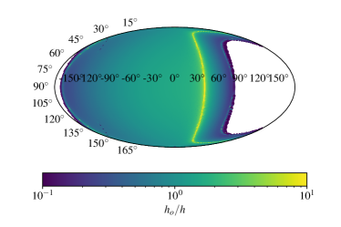
Figure 2: Dependence of the magnification factor $h_{o}/h$ on the direction $(\theta_{e},\phi_{e})$ of the ray when viewed in the rest frame of the source. The parameters are $a=0.9$ and $r_{s}=3M$.

We find the following interesting features in Figure 2. (i) The most obvious one is a large region with white color. This region corresponds to the directions in which the null geodesics eventually fall into the central SMBH (Igata et al., 2021). (ii) The edge of the white region becomes dark blue, indicating that the GWs in these directions are demagnified. In fact, many rays here can circle around the SMBH multiple times before they can escape to infinity. During this process, the magnification factor decays exponentially with the number of cycles the ray goes around the SMBH (Kocsis, 2013). (iii) Another prominent feature is a ring with bright yellow color circling the white region. The yellow color indicates large magnification. As we will show later, inside the ring neighbouring null geodesics will intersect. These behaviours resemble the behaviours of the light rays around a caustic in optics (Schneider et al., 1992; Hasse et al., 1996). For this reason, we call the bright yellow ring in Figure 2 “caustic” as well.

To better understand the cause of the caustic, we show in Figure 3 the evolution of the $\theta$ value of a null geodesic as it propagates to larger $r$. For illustrative purposes, we restrict ourselves to the rays close to the equatorial plane, i.e., we consider two different values of $\theta_{e}$, $90^{\circ}\pm\Delta\theta_{e}$ where $\Delta\theta_{e}\ll 10^{\circ}$. In addition, we choose three different $\phi_{e}$ directions (in the source frame), corresponding to the rays outside, close to and inside the caustic. We find that the rays close to the caustic (green solid lines) converge to nearly one point. That is why the magnification is high close to the caustic. Moreover, the rays inside the caustic (purple dash-dotted lines) intersect with the equatorial plane and end up in a hemisphere opposite to the one from which the rays originate.

Two additional features in Figure 2 are worth mentioning. (i) Between the bright yellow ring and the edge of the white region is another narrower yellow ring. We find that the geodesics starting from the region between the two yellow rings will intersect with their neighbour geodesics only in one direction, either $\theta$ or $\phi$. However, the geodesics inside the inner yellow ring can intersect with their neighbours in both directions. (ii) We also see several dark blue spots in the upper left and lower left directions. These rays are close to spherical photon orbits relative to the SMBH. They appear only when the source is inside the photon circular orbit in the retrograde direction. They also circle around the SMBH multiple times before escaping to infinity, which results in their strong demagnification.

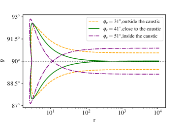
Figure 3: Evolution of the null geodesics close to the equatorial plane of the Kerr SMBH. Different line styles correspond to different initial $\phi_{e}$ values in the rest frame of the BBH.

Figure 4: Magnification $h_{o}/h$, seen by distant observers, as a function of the Boyer-Lindquist coordinates $(\theta,\phi)$ centred on the Kerr SMBH. The parameters are the same as in Figure 2. Here the inclination angle $\theta=90^{\circ}$ corresponds to the equatorial plane and we have chosen the azimuthal angle $\phi=0$ to be the direction of the orbital velocity of the BBH. In this coordinate system, an observer at $\theta=90^{\circ}$ and $\phi=90^{\circ}$ is on the opposite side of the SMBH when viewed form the BBH. . The left panel shows the rays starting from the exterior of the bright yellow circle (caustic) in Figure 2. The right panels shows the rays originating inside the caustic.

The above sky map of magnification is viewed in the source frame. When the rays arrive at a distant observer, however, the angular dependence of the magnification will look different due to the bending of the null geodesics around the SMBH. A natural coordinate system to visualize the distribution is the Boyer-Lindquist coordinate. Figure 4 shows the magnification as a function of the Boyer-Lindquist coordinate $(\theta,\phi)$ of the SMBH. The sky direction in this plot is directly connected to the line-of-sight of a distant observer. Notice that we have chosen $\phi=0^{\circ}$ to be the direction of the orbital velocity of the BBH in the Boyer-Lindquist coordinates. To see more clearly the role of the caustic, we plot in the left panel only those rays originating from the exterior of the caustic (out of the bright yellow ring in Figure 2). The rays originating inside the caustic are shown in the right panel.

From the left panel we see a pattern that is very different from Figure 2. We no longer see a large region with white color. Instead, we find white gaps, but they are numerical, caused by the limited number of rays that we have chosen. This result indicates that the distant observer can “see” the BBH from all angles. Even if the observer and the BBH are on opposite sides of the SMBH, one ray from the BBH can still go around the SMBH, due to the space-time curvature, and reach the observer.

From the same panel, we also find that the region of strong magnification ($h_{o}/h\simeq 10$) is concentrated in one direction, close to $\phi=120^{\circ}$ and $\theta=90^{\circ}$. Notice that there is a large offset between this direction of maximum magnification and the velocity of the BBH ($\theta=0$, $\phi=0$). The solid angle of this region where magnification is prominent is much smaller than the angular span of the caustic in the source frame. As we have shown earlier, the rays close to the caustic are strongly bent by the lensing effect, resulting in a significant shrinkage of the solid angle in the Boyer-Lindquist coordinate. The small solid angle in the SMBH’s frame also implies that the probability of seeing a highly beamed BBH is low. Far away from the direction of caustic, the magnification (or demagnification) factor remains moderate. This result suggests that outside the caustic the lensing effect is relatively mild.

The right panel of Figure 4 shows a much more complex pattern. While we still see a small region of strong magnification which is concentrated in one direction, we also find large demagnification ($h_{o}/h\simeq 0.1$) in a wide range of directions. This result suggests that the GWs originating inside the caustic could be strongly lensed and demagnified.

Comparing the sky maps in both panels, we find that in many sky directions a ray outside the caustic could coincide with a ray coming from inside the caustic. This coincidence implies that an observer in such a special direction can detect two images. Since these two images are emitted in very different directions in the rest frame of the source, they will show different magnification when detected by the observer. Therefore, the distance inferred from the two images will also differ, for the reason given in Section 2.1. This difference may further prevent us from finding echoes that are physically associated with the same source (e.g. Kocsis, 2013; Gondán & Kocsis, 2022; Yu et al., 2021), in addition to the reason we have pointed out in Section 2.3.

(a)	(b)	(c)

Figure 5: Mapping the rays just emitted in the source frame (panel a) to the rays arriving at a distant observer (panels b and c). Notice that in our model the rays arriving at a observer is viewed in the Boyer-Lindquist coordinates of the SMBH. The color shows the inclination angle $\theta_{e}$ of the ray in the source frame. Panel (b) shows only those rays outside the caustic and panel (c) shows the rays inside the caustic.

To better understand the cause of the complexity of the pattern we have just seen in the right panel of Figure 4, we show in Figure 5 a map of the rays from the source frame (panel a) to the SMBH’s frame (panels b and c). Here we use the inclination angle $\theta_{e}$ in the source frame to color code the map. We also separate the rays originating outside the caustic from those originating inside, and plot them in, respectively, panels (b) and (c).

First, by comparing panels (a) and (b), we find that the rays in the polar region of the source frame are compressed towards the equatorial plane in the SMBH’s frame.This is partly a consequence of the beaming effect, and partly due to the lensing effect. The comparison also shows that the rays originating outside the caustic do not cross the equatorial plane, i.e., those from the northern (southern) hemisphere in the source frame end up in the same hemisphere in the SMBH’s frame.

Panel (c), which shows the rays inside the caustic, depicts a very different picture. Now the colors in the two hemispheres are largely reversed relative to those in panel (a). This result suggests that most of the rays inside the caustic will cross the equatorial plane as they propagate to infinity.

(a)	(b)	(c)

Figure 6: The same as Figure 5 but color coded using the azimuthal angle $\phi_{e}$ in the source frame.

Figure 6 shows the same map but color coded by the azimuthal angle $\phi_{e}$ in the rest frame of the source. We see a behavior similar to that in Figure 5. When viewed in the SMBH’s frame, the rays outside the caustic (panel b) exhibit a smooth transition in color, except for a high concentration of bright yellow color in the direction of caustic. The rays inside the caustic (panel c), on the contrary, show a much more complicated pattern, which reflects the fact that they are crossing each other in the azimuthal direction.

3.2 Redshift as a function of viewing angle

The Doppler and gravitational redshifts of a ray seen by a distant observer depend only on the rescaled constant $b$ (Section 2.3). The combined redshift $(1+z_{\rm dop})(1+z_{\rm gra})$ is shown in Figure 7. The parameters and the meaning of each panel are the same as in Figure 5.

(a)	(b)	(c)

Figure 7: The same as Figure 5 but color coded by the combined redshift $1+z=(1+z_{\rm dop})(1+z_{\rm gra})$ due to the Dopper effect and the gravitational redshift.

In panel (a), the rest frame of the source, we can see a Doppler blueshift of the rays in the direction of the orbital velocity of the BBH. Correspondingly, the strongest redshift appears at $\phi_{e}\simeq 180^{\circ}$, opposite to the direction of the orbital velocity. Now we can see more clearly the asymmetry between redshift and blueshift caused gravitational redshift, which we have first mentioned in Section 2.3. More specifically, in this example the maximum redshift is $1+z\simeq 4.21$, while the maximum blueshift is about $1+z\simeq 0.67$.

In panel (b), which shows the observer’s view of the rays outside the caustic, we find that more than half of the sky is covered by redshift. This result reinforces the asymmetry between redshift and blueshift, and corroborates our earlier speculation that a BBH close to a SMBH is more likely to be seen redshifted. Comparing this panel with the left one in Figure 4, we also find a close correlation between redshift and demagnification. Since demagnification makes a BBH appear more distant (Section 2.1), we conclude that BBHs close to SMBHs will more often appear heavier and further away than they really are. It will be interesting to test such a positive correlation between mass and distance in real GW observations.

Panel (c) shows the observer’s view of the rays originating inside the caustic. Most of the rays are moderately redshifted or blueshifted, except for a few direction in which the rays get highly redshifted. Again, we find that the highly redshifted directions correspond to the directions of large demagnification. Observationally, this correspondence will produce a positive correlation between the mass and the distance of a BBH. Moreover, by comparing panels (b) and (c), we confirm the discovery made in Section 2.3 that in many direction the observer can detect two images with significantly different redshifts. Comparing Figures 4 and 7, we can see that outside the caustic, most rays which are moderately shifted in frequency are also moderately magnified. However, it is no longer the case for the rays inside the caustic, where many moderately Doppler shifted rays are highly demagnified. The difference indicates that the two groups of rays will occupy different regions in the diagram of $1+z$ and $h_{o}/h$. Therefore, their apparent mass and apparent distance will also follow different trends. We will see this more clearly in the following subsection.

So far we have only considered the system with the parameters $r_{s}=3M$ and $a=0.9$. To see the dependence of the combined redshift $1+z$ on these parameters, we show in Figure 8 the maximum and minimum values of $1+z$ as a function of $r_{s}$ and $a$. Notice that $1+z<1$ corresponds to a blueshift of GW, and the radius of the innermost stable circular orbit (ISCO) depends on $a$. We find that the value of $1+z$ is insensitive to the spin paramiter $a$, but more sensitive to the distance $r_{s}$ between the BBH and the SMBH. The dependence on $r_{s}$ is more prominent for redshifted rays (red symbols). When $r_{s}=(2.4,3,4.3,6,10)M$, the maximum redshift is $1+z_{\rm{max}}\simeq(6.10,4.21,2.64,2.02,1.60)$. These values suggest that a stellar-mass BH similar to those found in X-ray binaries (e.g., with a typical mass of $10M_{\odot}$) will appear significantly more massive (e.g., $20-60M_{\odot}$) in the rest frame of a GW detector. Interestingly, the apparent mass in this example seems to be consistent with the massive BHs detected by LIGO and Virgo.

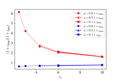
Figure 8: Dependence of the maximum redshift (red symbols) and maximum blueshift (blue symbols) on the radius of the source $r_{s}$ and the spin $a$ of the SMBH.

4 Appearance of a BBH close to a SMBH

In the previous sections, we have shown how a nearby SMBH affects the redshift and amplitude of the GW emitted by a BBH. In this subsection, we will further study the impact on the chirp mass $\mathcal{M}_{o}$ and apparent distance $d_{o}$ in the detector’s frame. We will also investigate the effects on the inferred parameters of the BBH, namely the inferred chirp mass $\mathcal{M}^{\prime}$ and the inferred redshift $z_{d_{o}}$. The latter two parameters are related to $\mathcal{M}_{o}$ and $h_{o}$ through Equations (4) and (5).

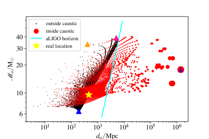
Figure 9: Distance and chirp mass of a BBH in the detector frame (see Section 2.1 for explanation). The dots correspond to those rays shown in Figure 4. Here we have also assumed that $m_{1}=m_{2}=10M_{\odot}$, and the SMBH resides at a cosmological redshift of $z_{\rm cos}=0.1$. The black dots correspond to the rays originating outside the caustic and the red ones inside the caustic. The size of a dot is proportional to the solid angle of the ray bundle in the Boyer-Lindquist frame, and hence is directly correlated with the probability of detecting the ray bundle. The yellow star marks the location of the BBH if there is no SMBH around the BBH. The cyan line shows the detection horizon of advanced LIGO (aLIGO). The four triangles are four representative images, which will be analyzed later to illustrate the dependence of the apparent mass and disntance on the real cosmological redshift of the source.

In Figure 3 we show the distribution of the rays emitted by one BBH in the plane of $d_{o}$ and $\mathcal{M}_{o}$. The black dots represent the rays outside the caustic and the red ones inside the caustic. The size of a dot represents the solid angle that the ray bundles span in the SMBH’s sky. Therefore, it is proportional to the possibility for an observer in an arbitrary direction to see the signal. Generally speaking, the the dots at larger $\mathcal{M}_{o}$ correspond to the rays that are more redshifted. Again, we can see the asymmetry between redshift and blueshift, since the majority of the dots lie above the real chirp mass (marked by the yellow star) of the BBH. Moreover, the dots at larger $d_{o}$ could also come from the rays that are significantly demagnified, since $d_{o}$ is proportional to the solid angle according to Equations (4) and (21). This effect produces those big red dots which occupy the right-half of the plot. We notice that the combined redshift $1+z$ is normally smaller than $10$ in our examples, but the apparent distance $d_{o}$ for some rays can be more than ten times greater than the real luminosity distance $d_{L}$ of the source. This discrepancy indicates that the large apparent distances are caused not by the redshift effect, but the lensing of the GWs by the SMBH.

If we focus on the rays outside the caustic (black dots), we find that they are aligned in the diagonal direction. Such a positive correlation between apparent mass and distance is caused by the fact that both parameters are positively correlated with the redshift (see Section 2.1). The rays originating outside the caustic (red dots) show a more complex distribution. In particular, there are many branches and they occupy a much larger parameter space. The overall shape of the distribution is also quite different from that of the black dots. This difference reflects the transition of the relationship between redshift and magnification as the rays enter the caustic, which we have already discussed in Section 3.2. Nevertheless, the positively correlation between apparent mass and apparent distance is still present.

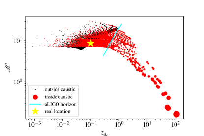
Figure 10: Apparent cosmological redshift and apparent chirp mass of a BBH inferred by an observer who does not know that the BBH resides close to a SMBH. The dots and their sizes have the same meanings as in Figure 3. The yellow star marks the real location of the BBH. The cyan solid line indicates the detection horizon of the advanced LIGO detectors.

Figure 10 shows the distribution of the rays in the $z_{d_{o}}$-$\mathcal{M}^{\prime}$ plane. Comparing with Figure 3, we first notice that the maximum $\mathcal{M}^{\prime}$ is significantly smaller than the maximum $\mathcal{M}_{o}$. The decrement is caused by the factor of $1+z_{d_{o}}$, as we have shown in Equation (6). We also notice that the distribution of the dots are much flatter in Figure 10 than in Figure 3. In particular, the big red dots, which correspond to the rays that are significantly demagnified, bend over and trace the off diagonal in Figure 10. The cause is the same as before, due to the correlation between demagnification and larger $1+z_{d_{o}}$. Interestingly, the biggest red dots occupy a region of large apparent redshift and small (sub-solar) BH mass. Such a region was thought to be occupied only by primordial black holes (Abbott et al., 2018). Unfortunately, the BBHs in this region are below the current detection limit.

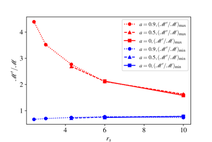
Figure 11: Dependence of the inferred mass on $r_{s}$ and $a$. Red dots show the maximum values of $\mathcal{M}^{\prime}/\mathcal{M}$ at the corresponding $r_{s}$, and the blue dots show the minimum values of $\mathcal{M}^{\prime}/\mathcal{M}$. We only include those rays detectable by aLIGO. The values of $r_{s}$ are $(2.4,3,4.3,6,10)M$. The real cosmological redshift of the source is set to $z_{\mathrm{cos}}=0.1$.

In Figure 11 we show the range of $\mathcal{M}^{\prime}/\mathcal{M}$ as a function of $r_{s}$ and $a$. Notice that when determining the minimum value of $\mathcal{M}^{\prime}/\mathcal{M}$, we have excluded the dots below the detection limit of aLIGO. Similar to Figure 8, the result is more sensitive to $r_{s}$ than to $a$. In this work we take $z_{\rm{cos}}=0.1$, and hence when $r_{s}=(2.4,3,4.3,6,10)M$ and $a=0.9$, the maximum values of $\mathcal{M}^{\prime}/\mathcal{M}$ are $(4.39,3.52,2.77,2.11,1.61)$. The corresponding minimum values are $(0.67,0.70,0.74,0.77,0.81)$. These values indicate that an observer unaware of the presence of the SMBH would overestimate (underestimate) the mass of the BBHs by a factor of $4.39$ ($0.67$).

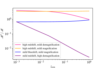
Figure 12: Dependence of $\mathcal{M}^{\prime}/\mathcal{M}$ on the real cosmological redshift of the source $z_{\rm{cos}}$. The four lines correspond to the four images marked by triangles in Figure 3. The paramters other than $z_{\rm{cos}}$ are the same as in Figure 3.

We notice that the value of $\mathcal{M}^{\prime}/\mathcal{M}$ depends on the choice of the real cosmological redshift $z_{\rm{cos}}$ of the source. The dependence is nonlinear due to the nonlinear relationship between $1+z_{\rm{cos}}$ and $1+z_{d_{o}}$. To illustrate the relationship, we show four examples in Figure 12. They are chosen from Figure 3, where the value of $z_{\rm{cos}}$ was fixed at $0.1$. Now we allow $z_{\rm{cos}}$ to change and study the variation of $\mathcal{M}^{\prime}/\mathcal{M}$. We find that if a ray gets magnified (orange and blue lines), the $\mathcal{M}^{\prime}/\mathcal{M}$ of the image will slightly increase with $z_{\rm{cos}}$. In this case, an ignorant observer may further overestimate the mass of the BBH if the system resides at higher cosmological redshift. For demagnified images (red and purple), the relationship reverses. Therefore, a BBH at lower cosmological redshift could appear more massive. In this case, we find that the maximum value of $\mathcal{M}^{\prime}/\mathcal{M}$ in our previous example becomes $5.61$ if we use $z_{\rm{cos}}=0.01$.

5 Discussion

In this work we have studied how the apparent mass and distance of a GW source (a BBH) would be affected by a nearby Kerr SMBH. Our study is motivated by the recent theoretical discovery that BBHs could merge within tens of gravitational radii of a SMBH (Chen & Han, 2018; Addison et al., 2019; Peng & Chen, 2021). We showed that the appearance of the BBH depends on the frequency shift and (de)magnification of the GW signal. By analyzing the null geodesics originating within $10$ gravitational radii of the SMBH, we found a higher probability for the GW signal to appear redshifted and demagnified, rather than blueshifted and magnified, when detected by a distant observer. Such an asymmetry indicates that the observer, unaware of the presence of the SMBH, is more likely to overestimate the mass and distance of the BBH.

Our examples suggest that a BBH residing at approximately the ISCO ($r_{s}\simeq 2.4$) of a Kerr SMBH ($a=0.9$) could appear $4.4-5.6$ times more massive than its real mass, if the systems resides at a cosmological redshift between $z_{\rm{cos}}=0.01$ and $0.1$. For this reason, a binary composed of normal stellar-mass BHs of $(10-20)M_{\odot}$ would appear to contain overly massive BHs, with a mass of $(40-110)M_{\odot}$. Interestingly, such massive BHs have been detected by LIGO/Virgo. For example, the rest mass of the primary BH of GW190521 is estimated to be $m_{1}=95.3^{+28.7}_{18.9}$, and that of GW190426_190642 is about $m_{1}=106.9^{+41.6}_{25.2}$ (The LIGO Scientific Collaboration et al., 2021a). It is still too early to conclude that GW190521 and GW190426_190642 are coming from the vicinities of SMBHs, since conventional models can also explain their existence (Romero-Shaw et al., 2020; Bustillo et al., 2021; De Luca et al., 2021; Fragione et al., 2020). However, the fact, that out of the $\sim 90$ BBHs detected so far by LIGO/Virgo two contain BHs of $\sim 100M_{\odot}$, is roughly consistent with the estimation that about $1\%$ of the LIGO/Virgo BBHs are produced at the inner edges of the accretion disks in AGNs (Peng & Chen, 2021).

One major difference between our work and the earlier ones on the magnification of GWs by SMBHs (e.g. Kocsis, 2013; Gondán & Kocsis, 2022; Yu et al., 2021) is that we studied the angular dependence of the gravitational lensing effect. Therefore, we found that in the majority of the directions the GWs will be, in fact, demagnified. We have shown that demagnified images could be misinterpreted as subsolar-mass BHs merging at $z_{\rm{cos}}>10$ (Figure 10), if the data analysis does not account for the presence of a nearby SMBH. Such events could be misidentified as primordial BHs produced by density fluctuation in the early universe (e.g. Abbott et al., 2018; Chen & Huang, 2020). Although these events fall below the sensitivity of the current detectors, they may be found by future ground-based detectors such as the Einstein Telescope and Cosmic Explorer (Punturo et al., 2010; Abbott et al., 2017).

It is known that an impulsive light source close to a SMBH can produce at least two images relative to a distant observer, a primary image corresponding to the ray going directly from the source to the observer and a secondary one caused by the ray going around the SMBH (e.g. Thompson, 2019). The same applies to a impulsive GW source, as we have shown in Figures 1, 4 and 7. We found that the two images will be redshifted and (de)magnified differently, because in the source frame they are emitted in two different directions and around the SMBH they follow different null geodesics. The difference in redshift and (de)magnified, according to the analysis in Section 2.1, will result in different apparent mass and distance for the two images. Therefore, an observer may interpret them as two physically separated, independent events.

Additional informational may help the observer realize that two events seemly uncorrelated by mass and distance may actually be the two images of the same BBH merger. First, the sky locations of the two images should be the same since the two images originate from the same galaxy. Second, there is a typical time delay of $\sim 10M\simeq 1.4M_{8}$ hours between the two images, where $M_{8}\equiv M/(10^{8}M_{\odot})$. The duration corresponds to the light crossing time over the region of strong lensing around the SMBH. Third, the two images should yield the same mass ratio $m_{2}/m_{1}$ for the BBH, since frequency shift and the lensing effect do not affect the measurement of this parameter (as long as the impulsive approximation of the signal is valid). Therefore, looking for correlated events in the three-dimensional space of sky location, signal arrival time and mass ratio could eventually reveal those BBHs close to SMBHs.

The impulsive approximation adopted by our model would break down if the SMBH is less massive than $10^{5}M_{\odot}$. In this case, the size of the ISCO is of the order of $10^{5}-10^{6}$ km and the BBH would have traversed a distance of $\sim c\times 0.1s\simeq 3\times 10^{4}$ km in the typical duration ($0.1$ s) of the signal. The latter is a substantial fraction of the former, indicating that the the velocity and the position of the BBH relative to the distant observer would have varied substantially during the time span of the signal. This variation effectively changes the view angle of the source by the observer. A change of the viewing angle will change the frequency and amplitude of the GW signal, as we have discussed extensively in Section 3. In addition, the plus and cross polarizations of the signal will also change because they also depend on the viewing angle.

We do not yet know whether the above effects could provide a potential signature for the observer to distinguish the BBHs around SMBHs from other isolated ones, because the effects related to a varying viewing angle can be mimicked by a precession of the orbit induced by, e.g., the spin of the BHs or the orbital eccentricity of the binary (Vecchio, 2004; Bustillo et al., 2021). Breaking such a degeneracy requires more careful modeling of the waveform of a BBH moving within a few gravitational radii of a Kerr SMBH (e.g. Cardoso et al., 2021).

Data Availability

The data underlying this article will be shared on reasonable request to the corresponding author.

References

- Abbott et al. (2017) Abbott B. P., et al., 2017, Classical and Quantum Gravity, 34, 044001
- Abbott et al. (2018) Abbott B. P., et al., 2018, Phys. Rev. Lett., 121, 231103
- Addison et al. (2019) Addison E., Gracia-Linares M., Laguna P., Larson S. L., 2019, General Relativity and Gravitation, 51, 38
- Antonini & Perets (2012) Antonini F., Perets H. B., 2012, ApJ, 757, 27
- Arca Sedda (2020) Arca Sedda M., 2020, ApJ, 891, 47
- Bardeen (1970) Bardeen J. M., 1970, ApJ, 162, 71
- Bardeen et al. (1972) Bardeen J. M., Press W. H., Teukolsky S. A., 1972, ApJ, 178, 347
- Bartos et al. (2017) Bartos I., Kocsis B., Haiman Z., Márka S., 2017, ApJ, 835, 165
- Baruteau et al. (2011) Baruteau C., Cuadra J., Lin D. N. C., 2011, ApJ, 726, 28
- Bonvin et al. (2017) Bonvin C., Caprini C., Sturani R., Tamanini N., 2017, Phys. Rev. D, 95, 044029
- Bozza (2008) Bozza V., 2008, Phys. Rev. D, 78, 103005
- Bozza & Mancini (2004) Bozza V., Mancini L., 2004, ApJ, 611, 1045
- Bustillo et al. (2021) Bustillo J. C., Sanchis-Gual N., Torres-Forné A., Font J. A., 2021, Phys. Rev. Lett., 126, 201101
- Campbell & Matzner (1973) Campbell G. A., Matzner R. A., 1973, Journal of Mathematical Physics, 14, 1
- Cardoso et al. (2021) Cardoso V., Duque F., Khanna G., 2021, Phys. Rev. D, 103, L081501
- Carter (1968) Carter B., 1968, Physical Review, 174, 1559
- Chen (2021) Chen X., 2021, in , Handbook of Gravitational Wave Astronomy. p. 39, doi:10.1007/978-981-15-4702-7_39-1
- Chen & Han (2018) Chen X., Han W.-B., 2018, Communications Physics, 1, 53
- Chen & Huang (2020) Chen Z.-C., Huang Q.-G., 2020, J. Cosmology Astropart. Phys., 2020, 039
- Chen & Zhang (2022) Chen X., Zhang Z., 2022, Phys. Rev. D, 106, 103040
- Chen et al. (2019) Chen X., Li S., Cao Z., 2019, Monthly Notices of the Royal Astronomical Society: Letters, 485, L141
- Corral-Santana et al. (2016) Corral-Santana J. M., Casares J., Muñoz-Darias T., Bauer F. E., Martínez-Pais I. G., Russell D. M., 2016, A&A, 587, A61
- Cunningham & Bardeen (1973) Cunningham C. T., Bardeen J. M., 1973, ApJ, 183, 237
- D’Orazio & Loeb (2020) D’Orazio D. J., Loeb A., 2020, Phys. Rev. D, 101, 083031
- De Luca et al. (2021) De Luca V., Desjacques V., Franciolini G., Pani P., Riotto A., 2021, Phys. Rev. Lett., 126, 051101
- Ford & McKernan (2021) Ford K. E. S., McKernan B., 2021, arXiv e-prints, p. arXiv:2109.03212
- Fragione et al. (2019) Fragione G., Grishin E., Leigh N. W. C., Perets H. B., Perna R., 2019, MNRAS, 488, 47
- Fragione et al. (2020) Fragione G., Loeb A., Rasio F. A., 2020, ApJ, 902, L26
- Gondán & Kocsis (2022) Gondán L., Kocsis B., 2022, MNRAS, 515, 3299
- Gralla & Lupsasca (2020) Gralla S. E., Lupsasca A., 2020, Phys. Rev. D, 101, 044032
- Gralla et al. (2018) Gralla S. E., Lupsasca A., Strominger A., 2018, MNRAS, 475, 3829
- Gröbner et al. (2020) Gröbner M., Ishibashi W., Tiwari S., Haney M., Jetzer P., 2020, A&A, 638, A119
- Hasse et al. (1996) Hasse W., Kriele M., Perlick V., 1996, Classical and Quantum Gravity, 13, 1161
- Holz & Hughes (2005) Holz D. E., Hughes S. A., 2005, ApJ, 629, 15
- Igata et al. (2021) Igata T., Kohri K., Ogasawara K., 2021, Phys. Rev. D, 103, 104028
- Inayoshi et al. (2017) Inayoshi K., Tamanini N., Caprini C., Haiman Z., 2017, Phys. Rev. D, 96, 063014
- Isaacson (1967) Isaacson R. A., 1967, Phys. Rev., 166, 1263
- Kocsis (2013) Kocsis B., 2013, ApJ, 763, 122
- LIGO Scientific Collaboration & Virgo Collaboration (2016) LIGO Scientific Collaboration Virgo Collaboration 2016, ApJ, 818, L22
- LIGO Scientific Collaboration & Virgo Collaboration (2020) LIGO Scientific Collaboration Virgo Collaboration 2020, ApJ, 900, L13
- Lawrence (1973) Lawrence J. K., 1973, Phys. Rev. D, 7, 2275
- Leigh et al. (2018) Leigh N. W. C., et al., 2018, MNRAS, 474, 5672
- Levin & Perez-Giz (2008) Levin J., Perez-Giz G., 2008, Phys. Rev. D, 77, 103005
- McClintock et al. (2014) McClintock J. E., Narayan R., Steiner J. F., 2014, Space Sci. Rev., 183, 295
- McKernan et al. (2012) McKernan B., Ford K. E. S., Lyra W., Perets H. B., 2012, MNRAS, 425, 460
- Meiron et al. (2017) Meiron Y., Kocsis B., Loeb A., 2017, ApJ, 834, 200
- Miller & Lauburg (2009) Miller M. C., Lauburg V. M., 2009, ApJ, 692, 917
- Misner et al. (1973) Misner C. W., Thorne K. S., Wheeler J. A., 1973, Gravitation
- O’Leary et al. (2009) O’Leary R. M., Kocsis B., Loeb A., 2009, MNRAS, 395, 2127
- Ohanian (1973) Ohanian H. C., 1973, Phys. Rev. D, 8, 2734
- Peng & Chen (2021) Peng P., Chen X., 2021, MNRAS, 505, 1324
- Pineault & Roeder (1977) Pineault S., Roeder R. C., 1977, ApJ, 212, 541
- Polnarev (1972) Polnarev A. G., 1972, Astrophysics, 8, 273
- Punturo et al. (2010) Punturo M., et al., 2010, Classical and Quantum Gravity, 27, 194002
- Romero-Shaw et al. (2020) Romero-Shaw I., Lasky P. D., Thrane E., Calderón Bustillo J., 2020, ApJ, 903, L5
- Rosquist et al. (2009) Rosquist K., Bylund T., Samuelsson L., 2009, International Journal of Modern Physics D, 18, 429
- Samsing et al. (2022) Samsing J., et al., 2022, Nature, 603, 237
- Sathyaprakash & Schutz (2009) Sathyaprakash B. S., Schutz B. F., 2009, Living Reviews in Relativity, 12, 2
- Schneider et al. (1992) Schneider P., Ehlers J., Falco E. E., 1992, Gravitational Lenses, doi:10.1007/978-3-662-03758-4.
- Schutz (1986) Schutz B. F., 1986, Nature, 323, 310
- Stone et al. (2017) Stone N. C., Metzger B. D., Haiman Z., 2017, MNRAS, 464, 946
- Tagawa et al. (2019) Tagawa H., Haiman Z., Kocsis B., 2019, arXiv e-prints, p. arXiv:1912.08218
- The LIGO Scientific Collaboration & The Virgo Collaboration (2019) The LIGO Scientific Collaboration The Virgo Collaboration 2019, ApJ, 882, L24
- The LIGO Scientific Collaboration & The Virgo Collaboration (2021) The LIGO Scientific Collaboration The Virgo Collaboration 2021, ApJ, 920, L42
- The LIGO Scientific Collaboration et al. (2021a) The LIGO Scientific Collaboration et al., 2021a, arXiv e-prints, p. arXiv:2108.01045
- The LIGO Scientific Collaboration et al. (2021b) The LIGO Scientific Collaboration the Virgo Collaboration the KAGRA Collaboration 2021b, arXiv e-prints, p. arXiv:2111.03606
- The LIGO Scientific Collaboration et al. (2021c) The LIGO Scientific Collaboration the Virgo Collaboration the KAGRA Collaboration 2021c, arXiv e-prints, p. arXiv:2111.03634
- Thompson (2019) Thompson C., 2019, ApJ, 874, 48
- Torres-Orjuela & Chen (2022) Torres-Orjuela A., Chen X., 2022, arXiv e-prints, p. arXiv:2210.09737
- Vecchio (2004) Vecchio A., 2004, Phys. Rev. D, 70, 042001
- Vijaykumar et al. (2022) Vijaykumar A., Kapadia S. J., Ajith P., 2022, MNRAS,
- Virbhadra & Ellis (2000) Virbhadra K. S., Ellis G. F. R., 2000, Phys. Rev. D, 62, 084003
- Weber (1970) Weber J., 1970, Phys. Rev. Lett., 25, 180
- Yang et al. (2019) Yang Y., Bartos I., Haiman Z., Kocsis B., Márka Z., Stone N. C., Márka S., 2019, ApJ, 876, 122
- Yu et al. (2021) Yu H., Wang Y., Seymour B., Chen Y., 2021, Phys. Rev. D, 104, 103011
- Zhang et al. (2021) Zhang F., Chen X., Shao L., Inayoshi K., 2021, ApJ, 923, 139