Systematic errors in the maximum–likelihood regression of Poisson count data: introducing the overdispersed $\chi^{2}$ distribution

Abstract

This paper presents a new method to estimate systematic errors in the maximum–likelihood regression of count data. The method is applicable in particular to X–ray spectra in situations where the Poisson log–likelihood, or the Cash goodness–of–fit statistic, indicate a poor fit that is attributable to overispersion of the data. Overdispersion in Poisson data is treated as an intrinsic model variance that can be estimated from the best–fit model, using the maximum–likelihood $C_{\text{min}}$ statistic. The paper also studies the effects of such systematic errors on the $\Delta C$ likelihood–ratio statistic, which can be used to test for the presence of a nested model component in the regression of Poisson count data. The paper introduces an overdispersed $\chi^{2}$ distribution that results from the convolution of a $\chi^{2}$ distribution that models the usual $\Delta C$ statistic, and a zero–mean Gaussian that models the overdispersion in the data. This is proposed as the distribution of choice for the $\Delta C$ statistic in the presence of systematic errors. The methods presented in this paper are applied to XMM–Newton data of the quasar 1ES 1553+113 that were used to detect absorption lines from an intervening warm–hot intergalactic medium (WHIM). This case study illustrates how systematic errors can be estimated from the data, and their effect on the detection of a nested component, such as an absorption line, with the $\Delta C$ statistic.

1 Introduction

The launch of the first satellites dedicated to the detection of X–rays beyond the Solar system, namely Uhuru (Giacconi et al., 1971) and the HEAO missions (Rothschild et al., 1979), marked the beginning of the field of X–ray astronomy in earnest. It soon became apparent that the new data provided by these instruments, typically in the form of the number of counts or photons as a function of time and energy, required new statistical tools for a proper analysis and interpretation. These new data led to several advances in the study of statistics for count data.

Among the tools needed to interpret the early X–ray data is the application of the maximum–likelihood method, devised decades earlier by R.A. Fisher (e.g. Fisher, 1922, 1934), to these inherently Poisson–distributed integer–count data. For normally distributed data, the maximum–likelihood method leads to the $\chi^{2}$ statistic that features relatively simple mathematical properties that have long been used by statisticians (e.g. Greenwood & Nikulin, 1996). For Poisson data, X–ray astronomer W. Cash was the first to show that it is possible to use the maximum–likelihood method to derive another statistic that is asymptotically distributed like a $\chi^{2}$ distribution. This statistic is now usually referred as the Cash statistic or $C$–stat (Cash, 1976, 1979), and it was further developed by Baker & Cousins (1984) and others. In other fields of statistics, an equivalent Poisson–based log–likelihood is referred to as the deviance of the Poisson log–likelihood (e.g. McCullagh & Nelder, 1989; Cameron & Trivedi, 2013), or the G–squared statistic (Bishop et al., 1975).

The consistent use of the $\chi^{2}$ statistic for integer–count data, in X–ray astronomy and in related field, is based on the fact that a Poisson distribution is known to be well approximated by a Gaussian in the limit of a large number of counts.  However, it has now become clear that, even in the large–count limit, minimization of the $\chi^{2}$ statistic for parameter estimation in models with free parameters will lead to biased results, when applied to Poisson data (e.g. Humphrey et al., 2009; Bonamente, 2020). Such bias is due to the fact that the $\chi^{2}$ statistic requires an estimate for the data variance (i.e., according to the modified $\chi^{2}$ minimum method described by Cramer, 1946, pp. 424-434), and using the number of counts as its estimate leads to a heavier weight being given to low–count datapoints in the process of the regression.

On the other hand, the $C$–stat does not have this bias, and it should be regarded as the statistic of choice for the majority of count data that are commonplace in X–ray astronomy and related fields. In fact, the major X–ray fitting packages (XSPEC and SPEX) now give the option to use either statistic (Arnaud, 1996; Kaastra et al., 1996), and SPEX also provides an estimate of the expected $C$–stat, under the assumption that the data follow the best–fit model, based on the approximations of Kaastra (2017). Nonetheless, the use of the $C$–stat for spectral fitting and other like applications remains hampered by its somewhat more complex mathematics. For example, even in the case of a simple linear regression, a fit to Poisson data does not have the type of simple analytical solution as in the case of the $\chi^{2}$ statistic, although it was recently shown to have a semi–analytical solution that can be easily implemented numerically (Bonamente & Spence, 2022).

In this paper we address an outstanding issue in the fit of integer–count data with the $C$–stat, namely how to measure possible systematic errors that go beyond the usual Poisson uncertainties. Unlike the case of Gaussian data fit with a $\chi^{2}$ statistic, where systematics can be immediately handled with traditional quadratue addition of errors, the Poisson–based $C$–stat offers no such direct modification. Instead, the problem can be approached with the use of an intrinsic model variance that reflect the presence of uncertainties in the best–fit model, instead of additional errors in the data.

This paper is structured as follows: Sect. 2 presents the statistical properties of the data model under consideration, and Sect. 3 presents the new method to address systematic errors with the Cash statistic, which includes the introduction of the overdispersed $\chi^{2}$ distribution. Sect. 4 illustrates the method with a case study with the XMM–Newton data for the source 1ES 1553+113 recently studied by Nicastro et al. (2018) and Spence et al. (2023), and Sect. 5 presents our conclusions.

2 Data models for count data

The data model considered in this paper is $N$ independent measurements of the type

$$(x_{i},y_{i})\;\text{ for }i=1,\dots,N,$$ (1)

where $x_{i}$ is an independent variable assumed to be known exactly (e.g., the wavelength or the energy of the photons) and $y_{i}$ is an integer number of counts (e.g., the number of counts or photons in a given bin). This is the standard model for astronomical X–ray spectra, but also applies to a variety of data from other fields, and it is often referred to as cross–sectional data. These data are fit to a parametric model $y=f(x)$, where the function $f(x)$ has $m$ free parameters to be determined according to the maximum–likelihood method.

2.1 The standard Poisson model

The simplest assumption used to estimate model parameters is that the dependent variable $y_{i}$ is distributed like a Poisson variable,

$$y_{i}\sim\text{Poiss}(\mu_{i}),$$ (2)

with an unknown parent mean $\mu_{i}=\mu_{i}(x_{i})$ that is a function of a number of adjustable parameter $\theta_{j}$, $j=1,\dots,m$, and of the independent variable. Common situations in X–ray astronomy are power–law models, or thermal models that are a function of a handful of parameters such as temperature and chemical abundances, and more complex models that include absorption lines etc. etc. In all cases, the key assumption of this data model is the Poisson distribution of the number of counts that are detected in a given bin, i.e., a range in the $x$ variable that is represented by the characteristic value $x_{i}$.

Parameter estimation for these data are obtained from the usual maximum–likelihood method pioneered by R.A. Fisher (e.g., see Fisher, 1934), in this case making use of the Poisson distribution of the data and of the independence among the measurements. Under these assumptions, the relevant statistic to be minimized to obtain the best–fit parameters an their covariance matrix is the Cash statistics or $C$–stat, defined by

$$C=2\sum_{i=1}^{N}\left(\mu_{i}-y_{i}+y_{i}\ln\left(\dfrac{y_{i}}{\mu_{i}}\right)\right).$$ (3)

This statistic was developed by Cash (1976, 1979) and Baker & Cousins (1984), and it has the convenient property that it is asymptotically distributed as a $\chi^{2}$ distribution for a large number of counts per bin,

$$C\overset{a}{\sim}\chi^{2}(N)$$ (4)

when the model is fully specified (e.g., Kaastra, 2017; Bonamente, 2020, 2022). For a model with $m$ adjustable parameters, the maximum–likelihood regression with the Poisson statistic leads to the $C_{\text{min}}$ goodness–of–fit statistic,

$$C_{\text{min}}=2\sum_{i=1}^{N}\left(\hat{\mu_{i}}-y_{i}+y_{i}\ln\left(\dfrac{y_{i}}{\hat{\mu_{i}}}\right)\right),$$ (5)

where $\hat{\mu_{i}}$ is evaluated for the best–fit parameters $\hat{\theta}_{j}$. Its asymptotic distribution for a large number of counts per bin was shown by McCullagh (1986) to be approximately

$$C_{\text{min}}\overset{a}{\sim}\chi^{2}(N-m).$$ (6)

This asymptotic property is convenient for parameter estimation and for hypothesis/model testing (see, e.g., Kaastra 2017), and it is akin to a similar result that applies to the $\chi^{2}_{\text{min}}$ statistic (Cramer, 1946).

2.2 The overdispersed Poisson model

The greatest restriction imposed by the Poisson distribution is that the variance is equal to the mean,

$$\text{Var}(y_{i})=\mu_{i},$$ (7)

where $\mu_{i}$ is the parent mean of the data–generating process for the $i$–th bin. A common occurrence in datasets across the sciences, including astronomy, is that the measured data are overdispersed relative to the simple assumption on (7), e.g., see discussion in Chapter 3 of Cameron & Trivedi (2013). Reasons for this larger–than–${\mu_{i}}$ variance in the data include the inadequacy of the model — i.e., more explanatory variables may be required for multi–variable regression, or better parameterization of the model — or an intrinsic model variability that makes each independent measurement $y_{i}$ have a larger–than–Poisson variance.

Regardless of origin, overdispersion can be modelled via a function

$$\text{Var}(y_{i})=\omega_{i}=\omega(\mu_{i},\alpha)$$ (8)

that introduces an additional degree of freedom in the form of the parameter $\alpha$. While in principle the function can have any form, two convenient parameterizations proposed by Cameron & Trivedi (2013) are

$$\begin{cases}\begin{aligned} \omega_{i}&=(1+\alpha)\mu_{i}\;&\text{ (NB1 model)}\\ \omega_{i}&=\mu_{i}+\alpha\mu_{i}^{2}\;&\text{ (NB2 model)}\end{aligned}\end{cases}$$ (9)

where the model names derive from their use in the negative binomial regression by Cameron & Trivedi (1986). This paper does not make use of the negative binomial distribution, which is featured in an alternative method of regression for count data (e.g., see Hilbe, 2011, 2014), yet this parameterization remains applicable. When $\alpha=0$, the model returns the usual Poisson regression. When $\alpha>0$, on the other hand, the data no longer follows the Poisson distribution. In principle, it is also possible to have $\alpha<0$, which corresponds to underdispersed data. This case, however, occurs less often in practice, and (9) are normally used for $\alpha>0$. An equivalent parameterization for the NB1 model that is common in the generalized linear model (GLM) literature (e.g. McCullagh & Nelder, 1989) is to set

$$\phi=(1+\alpha)$$ (10)

with $\phi>1$ indicating overdispersed data.

The choice to allow overdispersion in the data means that minimization of the statistic described by (3) no longer represents a maximum–likelihood condition, since the data are no longer Poisson–distributed. Fortunately, there are situations when the usual Poisson regression, with best–fit parameters $\hat{\theta}_{j}$ obtained from the minimization of (3), continue to apply to the overdispersed Poisson model. In particular, Gourieroux et al. (1984b) have shown that, for a family of exponential distributions that includes the Poisson, the best–fit parameters estimated via the usual likelihood remain consistent even when the distribution is misspecified, provided that the mean is correctly specified. In this case, the method of estimation is referred to as a quasi maximum likelihood. 

In practice, these results let us continue with the usual Poisson likelihood under the assumption that the Poisson mean is correct. The problem then turns to the estimate of the overdispersion parameter $\phi$ defined in (10). The best–fit parameters from the Poisson quasi–ML method are asymptotycally normally distributed, with a variance that clearly depends on $\phi$ (see, e.g., Cameron & Trivedi, 2013). For the data analyst, what is of most interest is an estimate of the degree of overdispersion in the count data. The standard estimators for $\phi$ and $\alpha$ in the two models for the data variance in (9) are

$$\begin{cases}\begin{aligned} \hat{\phi}_{\text{NB1}}&=\dfrac{1}{N-m}\sum_{i=1}^{N}\dfrac{(y_{i}-\hat{\mu_{i}})^{2}}{\hat{\mu_{i}}}\\ \hat{\alpha}_{\text{NB2}}&=\dfrac{1}{N-m}\sum_{i=1}^{N}\dfrac{(y_{i}-\hat{\mu_{i}})^{2}-\hat{\mu_{i}}}{\hat{\mu_{i}}^{2}}.\end{aligned}\end{cases}$$ (11)

Justification for these estimators is provided in Cameron & Trivedi (2013); Gourieroux et al. (1984b, a), although other estimators are also available (see, e.g., Cameron & Trivedi, 1986; Dean & Lawless, 1989; Dean, 1992). The two equations in (11) provide point estimates for the overdispersion in count data, according to the alternative parameterizations of (9). Uncertainties in these estimates can be provided by standard error–propagation methods (also known as the delta method). A value $\hat{\phi}_{\text{NB1}}>1$ or $\hat{\alpha}_{\text{NB2}}>0$ indicates overdispersion in the data.

2.3 The Gaussian model

For X–ray spectral analysis, the use of the $\chi^{2}$ statistic remains pervasive, even for Poisson–distributed data. The $\chi^{2}$ goodness–of–fit statistic results from the use of an alternative data model, whereby the same data as (1) presume a parent distribution

$$y_{i}\sim\text{Gauss}(\mu_{i},\sigma^{2}_{i})$$ (12)

where a parent variance $\sigma^{2}_{i}$ is also required, in addition to the usual parent mean $\mu_{i}$. The widespread use of the $\chi^{2}$ fit statistic for integer–valued count data is primarily due to its ease of use and interpretation. This includes a reduction–of–degrees–of–freedom theorem established by H. Cramer (Cramer, 1946), which establishes the distribution of the $\chi^{2}_{\text{min}}$ statistic as

$$\chi^{2}_{\text{min}}\sim\chi^{2}(N-m),$$ (13)

where $m$ is the number of free parameters in the model and $N$ the usual number of independent Gaussian–distributed data points. This result holds under rather general conditions that are usually satisfied by X–ray astronomical data. 

The parent variance in (12) is usually approximated via the data variance, typically the number of counts in the bin, $\hat{\sigma}_{i}^{2}={n_{i}}$ (see, e.g. Bevington & Robinson, 2003; Bonamente, 2022). This approximation follows the Cramer (1946) modified minimum $\chi^{2}$ criterion, whereby the asymptotic distribution (13) holds under the assumption of a fixed data variance. It has been documented in the astronomical statistical literature that, even in the large–count limit where a Poisson distribution is in fact well approximated by the normal distribution, the use of the $\chi^{2}$ distribution leads to biased results, compared to the use of the $C$–stat (e.g. Humphrey et al., 2009; Bonamente, 2020). This is primarily due to the approximation of the variance in the data model (12) with a number that is smaller for bins with lower count–rates, which unduly carries a larger weight in the regression.

2.4 Regression with other distributions

Another possibility is to assume that the data follow an alternative distribution, such as the Conway–Maxwell–Poisson distribution (e.g. Conway & Maxwell, 1962; Shmueli et al., 2005; Sellers & Shmueli, 2010), the generalized Poisson distribution (e.g. Consul & Jain, 1973; Famoye, 1993), or the negative binomial distribution (e.g. Hilbe, 2011, 2014). These distributions introduce additional parameters that can conveniently model the data variance and thus allow for over– or under–dispersed data. Such modifications, however, come at a cost in terms of ease of use and interpretation, including the identification of an alternative goodness–of–fit statistic in place of the Poisson–based deviance or $C$–stat.

It is often preferrable to retain the Poisson distribution for the analysis of astronomical data, given its relative ease of use and the fact that most datasets are believed to be derived from a Poisson process with a fixed rate $\mu_{i}$. This paper therefore continuess with the assumption that the data are Poisson–distributed, and develop a new method that accounts for overdispersion.

3 Systematic errors in the maximum–likelihood regression of Poisson–distributed count data

It is traditional in X–ray astronomy and related fields to consider two separate types of uncertainties in the measurement of the $y_{i}$ data. The first is a so–called statistical error, typically used to denote the uncertainty associated with the photon–counting experiment (e.g., the square root of the number of counts). All other sources of uncertainty are often referred to as systematic errors, although they may well be errors that are random in nature in the same way as the photon–counting process itself. Examples of the latter type of errors are uncertainties associated with other aspects of the photon–collection process, such as uncertainties associated with the calibration of the instrument, or with other aspects of the analysis. What generally distinguishes the first from the second type of error is that the first are inherent in the collection process (i.e., in the Poisson distribution that underlies the $y_{i}$ variable), while the second can often be reduced by a careful reduction and analysis of the data. Although this distinction is somewhat arbitrary, it will be used in the remainder of this paper.

The usual method to address the presence of additional sources of systematic errors with the $\chi^{2}$ statistic for Gaussian data is to modify the variance in (12) until the fit statistic $\chi^{2}$ becomes ‘acceptable’. This method leverages the fact that the variances $\sigma^{2}_{i}$ are specifically part of the data model, per (1) and (12). A review of these methods is provided, for example, in Ch. 17 of Bonamente (2022), or in the textbook by Bevington & Robinson (2003). Prior to continuing the discussion of systematic errors, it is necessary to emphasize the meaning of the word acceptable when used in conjunction with hypothesis testing. Hypothesis testing is a process whose outcome is that of either discarding a null hypothesis at a given level of significance, or merely failing to discard it (see, e.g., the recent statemente by the American Statistical Association on $p$ values and hypothesis testing, Wasserstein & Lazar 2016). It is nonetheless reasonable to say that a hypothesis is acceptable when one may not reasonably discard it (say, at the 3 or 5 $\sigma$ level of confidence), provided it is understood that the hypothesis may never be conclusively accepted as the only possible model for the data.

For the type of Poisson data that are of common occurrence in X–ray astronomy, i.e., data following the assumption (2) and the resulting $C$–stat fit statistic (3), this direct avenue is not possible. The reason is that the variance of a Poisson data point is equal to its mean, and one may not independently specify both, as one can for the Gaussian distribution and the associated $\chi^{2}$ statistic according to (12). A convenient workaround that is well established in the statistical literature is the overdispersed Poisson regression that was discussed in Sect. 2.2. This quasi–ML method provides a convenient means to retain the Poisson–based maximum–likelihood best–fit statistic (i.e., the deviance or $C$–stat), while providing an estimate for the degree of overdispersion.

Within this statistical framework, this paper presents a new method to address the presence of overdisperion in count data and its effects on the Cash statistic. The method is based on the interpretation of the overdispersion as an intrinsic model variance that is modelled by an appropriate normal distribution of zero mean. Following this assumption, this additional source of uncertainty in the model is folded with the distribution for the usual Poisson–based $C$–stat, resulting in a modified distribution that can be used for the hypothesis testing of regression with overdispersed Poisson data. This method is described in the remainder of this section.

3.1 Measurement of the intrinsic model variance with the Cash statistic

The means to estimate systematic errors in Poisson–distributed data that are fit to a parametric model, as is customary in X–ray astronomy, is provided by a change in perspective with regards to the roles played in the regression by the data and the model. Specifically, instead of requring that the data points $y_{i}$ have a larger variance than what is estimated by their Poisson distribution, it is reasonable to assume that the model has an intrinsic variance. In practice, this means assuming that the parent model $\mu_{i}$ of a given datum $y_{i}$ is not a fixed (and unknown) number, as implied by its Greek–letter notation, but it follows a distribution with a given variance, or

$$\mu_{i}\sim\text{Gauss}(\mu_{i0},\sigma_{\text{int},i}^{2}),$$ (14)

where $\mu_{i0}$ is a parent value, $\sigma_{\text{int},i}^{2}$ is the intrinsic variance, and $i$ denotes the bin. This assumption is akin to what is done in the case of systematic errors for normal data – i.e., when the variance of the data are increased – except that the additional source of variance is now associated with the model, and not the data. Of course the intrinsic variance is not known a priori, but must be estimated from the data. This is similar to the case of the overdispersed Poisson model (see Sect. 2.2) which requires an estimate for the overdispersion parameters $\phi$ or $\alpha$.

To estimate the intrinsic variance in the model, it must be assumed that the best–fit model is an acceptable description of the data. In statistical terms, this null hypothesis can be rephrased as the requirement that the data are compatible with being drawn from the parent model, as measured from the fit statistic of choice, and at a given level of confidence. Given that the fit statistic of choice for Poisson data is $C_{\text{min}}$ according the (5), the model acceptability can be stated in terms of the requirement that the measured $C_{\text{min}}$ is statistically consistent with its parent distribution, under the null hypothesis. In the asymptotic limit of a large number of counts per bin, and regardless of the number of degrees of freedom, McCullagh (1986) showed that the statistic converges towards a $\chi^{2}$ distribution, namely

$$C_{\text{min}}\overset{a}{\sim}\chi^{2}(\nu)$$ (15)

where $\nu=N-m$ is the number of degrees of freedom. The proof provided by McCullagh (1986) assumes that the model is linear (or, more precisely, log–linear), and it is based on the calculation of conditional cumulants (McCullagh, 1984), and therefore the extrapolation to non–linear models such as the one used in Spence et al. (2023) would require further theoretical justification. To the best of the author’s knowlegde, to date a general proof of (15) for a general non–linear model has not been obtained, but it will be hereafter assumed as a first–order approximation for a general non–linear model.

Another important caveat is that, in the low–count regime, (15) will in general not apply, and additional considerations need to be used. A discussion of the distribution of $C_{\text{min}}$ in the low–count and few–bin regimes is also provided in McCullagh (1986), and also in Bonamente (2020) and Kaastra (2017). Qualitatively speaking, (15) is understood with the convergence of the Poisson distribution to a normal distribution in the large–count limit. For clarity, the domains of applicability of the results provided in this paper will be summarized in Sect. 3.3.

3.1.1 The asymptotic distribution of $C_{\text{min}}$ with systematic errors

The problem now turns to the determination of the effect of the intrinsic model variance (14) on the asymptotic distribution of $C_{\text{min}}$, obtained under the assumption of Poisson measurements. For this purpose, we make the following approximations, which correspond to common experimental conditions:

(a) For a large value of the number of degrees of freedom, the $\chi^{2}(\nu)$ distribution is equivalent to a $N(\nu,2\nu)$ normal distribution, especially for large values of the statistic that are not affected by the positive–definite nature of the $\chi^{2}$ distribution. This is consistent with (15), for large $\nu$. The case of a small $\nu$ is addressed in Sect. 3.2, which describes the effect of intrinsic variance on the $\Delta C$ statistic.

(b) We assume small values for the intrinsic variance, $\sigma_{\text{int},i}/\mu_{i0}\ll 1$, meaning that there is a small fractional systematic error. Accordingly, the method uses a simple error–propagation or delta method to estimate the additional variance to the $C_{\text{min}}$ statistic introduced by the assumption (14).

(c) Following the two earlier assumption, the systematic error (or, more precisely, the intrinsic variance) according to (14) leads to a $Z=C_{\mathrm{min}}$ statistic that can be thought of as the sum of two independent variables, $Z=X+Y$, with

$$\begin{cases}X\sim\chi^{2}(\nu)\overset{a}{\sim}N(\nu,2\nu)\\ Y\sim N(0,\hat{\sigma}^{2}_{C}),\end{cases}$$ (16)

with $\nu=N-m$. The null mean for $Y$ means that the systematic error does not provide a net mean value or bias to the statistic, and $\hat{\sigma}^{2}_{C}$ represents an additional variance term of $C_{\text{min}}$ associated with the systematic errors, which will be estimated from the data. This ensures that the modified distribution for the $C_{\text{min}}$ statistic remains approximately normal, with increased variance relative to the standard Poisson regression.

3.1.2 The estimation of the intrinsic variance

The model described in the previous section has introduced two quantities, the intrinsic model variance $\sigma_{\text{int},i}^{2}$ and a ‘design’ variance of the $C_{\text{min}}$ statistic $\hat{\sigma}^{2}_{C}$ that is required for acceptability of the null hypothesis. This section addresses their estimates.

For a given application, the first step is the estimate of the required intrinsic variance for the fit statistic, which is denoted by

$$\text{Var}_{i}(C_{\text{min}})=\hat{\sigma}^{2}_{C}.$$ (17)

The meaning of (17) is that the $C_{\text{min}}$ statistic requires an additional variance, in a given amount of $\hat{\sigma}^{2}_{C}$, in order for the measured statistic to be consistent with its expectation under the null hypothsis. According to (16), the total variance of the $C_{\text{min}}$ statistic is then

$$\text{Var}(C_{\text{min}})=2\nu+\hat{\sigma}^{2}_{C},$$ (18)

with the assumption that the $C_{\text{min}}$ statistic retains the normal distribution, in the asymptotic limits of a large number of counts per bin, and a large number of bins.

The problem now turns to the evaluation of the left–hand term of (17), and its relationship to the sought–after intrinsic model variance $\sigma_{\text{int},i}^{2}$ in (14). The intrinsic model variance can be evaluated following its definition of

$$\text{Var}_{i}(C_{\text{min}}) =\text{E}\left[\left(C_{\text{min}}(\mu_{i})-\text{E}\left[C_{\text{min}}(\mu_{i})\right]\right)^{2}\right]$$ (19)

$$\simeq\text{E}\left[\left(C_{\text{min}}(\mu_{i})-C_{\text{min}}(\hat{\mu_{i}})\right)^{2}\right],$$

with the approximation of $\text{E}\left[C_{\text{min}}(\mu_{i})\right]\simeq C_{\text{min}}(\hat{\mu_{i}})$. The meaning of (19) is that $\mu_{i}$ is a considered a random variable, distributed according to (14), while $\hat{\mu_{i}}$ is the usual maximum–likelihood estimate. In other words, this variance is calculated with respect to the distribution (14), and not with respect to the distribution of the data according to (2) — this is the reason for the $i$ subscript in the notation of the variance of (17) and (19). In fact, the Poisson distribution for the data $y_{i}$ is responsible for the variance of $C_{\text{min}}$ that was already calculated, i.e., using the large–count approximation as in (15), or according to the methods of Kaastra (2017) for the low–count regime.

To evaluate (19), use the $C$–stat defined in (3),

$$C_{\text{min}}(\mu_{i})-\text{E}\left[C_{\text{min}}\right]=2\left(\sum_{i=1}^{N}(\hat{\mu}_{i}-\mu_{i})+y_{i}\ln\left(\dfrac{\mu_{i}}{\hat{\mu}_{i}}\right)\right)$$

$$\simeq 2\left(\sum_{i=1}^{N}(\hat{\mu}_{i}-\mu_{i})+y_{i}\left(\dfrac{\mu_{i}-\hat{\mu}_{i}}{\hat{\mu_{i}}}\right)\right)=2\left(\sum_{i=1}^{N}(\mu_{i}-\hat{\mu}_{i})\left(\dfrac{y_{i}}{\hat{\mu}_{i}}-1\right)\right)$$

where it was assumed a small value for the fractional intrinsic error, $\sigma_{\text{int},i}/\mu_{i}$, so that only the first–order term in the Taylor series expansion of the logarithm was retained. With this approximation, (19) leads to

$$\text{Var}_{i}(C_{\text{min}})\simeq\text{E}\left[\left(2\sum_{i=1}^{N}(\mu_{i}-\hat{\mu_{i}})\underbracket{\left(\dfrac{y_{i}}{\hat{\mu_{i}}}-1\right)}_{(a)}\right)^{2}\right],$$ (20)

where the term $(a)$ highlighted by the square bracket is independent of $\mu_{i}$. Moreover, upon evaluation of the square of the sum, the cross–product terms have null expectation, under the assumption that the $\mu_{i}$ terms are uncorrelated. This leads to the simple result that

$$\text{Var}_{i}(C_{\text{min}})=\hat{\sigma}^{2}_{C}\simeq 4\left(\sum_{i=1}^{N}\sigma_{\text{int},i}^{2}\left(\dfrac{y_{i}}{\hat{\mu_{i}}}-1\right)^{2}\right),$$ (21)

with the intrinsic variance of the model being

$$\sigma_{\text{int},i}^{2}=\text{E}[(\mu_{i}-\hat{\mu_{i}})^{2}].$$

The right–hand term of (21) can be further approximated by the assumption that $y_{i}\sim\text{Poiss}(\hat{\mu_{i}})$, i.e., it is true that, on average

$$(\hat{\mu_{i}}-y_{i})^{2}\simeq\hat{\mu_{i}}\simeq y_{i}.$$

Further assuming that the intrinsic fractional error is the same for all datapoints, i.e., $\sigma_{\text{int},i}/\hat{\mu_{i}}$ is a constant, we obtain the final result

$$\dfrac{\sigma_{\text{int},i}}{\hat{\mu_{i}}}\simeq\dfrac{1}{2}\dfrac{\hat{\sigma}_{C}}{\sqrt{\sum_{i=1}^{N}y_{i}}}.$$ (22)

Equation 22 is the sought–after result, namely the approximation that relates the fractional intrinsic scatter of the model (${\sigma_{\text{int},i}}/{\hat{\mu_{i}}}$) to the design value $\hat{\sigma}^{2}_{C}$ required for consistency between the measured $C_{\text{min}}$ and its parent distribution under the null hypothesis.  This approximation provides a simple means to estimate an average fractional or percent intrinsic variance of the model that is required to assure an acceptable fit.

3.2 The intrinsic model variance for hypothesis testing of a nested component with the $\Delta C$ statistic

The intrinsic model variance estimated from the $C_{\text{min}}$ statistic according to (22) makes it such the expected statistic, under the null hypothesis, is now consistent with the measured value. In fact, the method of estimation started with the requirement (17), designed exactly to achieve such agreement. Sect. 4 will present a detailed case study of how such estimate is performed in practice. In other words, the intrinsic model variance assumes that the fit is acceptable, and therefore hypothesis testing with $C_{\text{min}}$ is no longer meaningful.

Another common use of the $C_{\text{min}}$ statistic, also shared by the $\chi^{2}_{\text{min}}$ statistic, is when the statistic

$$\Delta C=C-C_{\text{min}}$$ (23)

is used to test the significance of a nested model component. This method was originally developed by Lampton et al. (1976) for the $\Delta\chi^{2}$ statistic, and it is based on the theory presented in Cramer (1946). A description of the $\Delta C$ statistic is presented in Ch. 16 of Bonamente (2022), with the main result of

$$\Delta C\overset{a}{\sim}\chi^{2}(l)$$ (24)

in the asymptotic limit of a large number of measurements, and with $l$ interesting (or free) parameters for the nested component.

The use of the $\Delta C$ statistic consists of calculating the $C_{\text{min}}$ fit statistic for the full model that includes a nested component, and the calculating the $C$ statistic with the nested model component zeroed–out (referred to as the reduced model), so that clearly $C\geq C_{\text{min}}$ and $\Delta C\geq 0$. In this case, the best–fit model $\hat{\mu_{i}}$ has $l$ additional parameters associated with its nested component, with a model value of $\mu_{i}^{{}^{\prime}}$ when the nested component is zeroed out. This is the case, for example, for the data of Tables 5 and 6 in Spence et al. (2023), where the $\Delta C$ values correspond to setting to zero a spectral line component that has $l$=1 or 2 additional free parameters, relative to a model for the continuum emission of a bright X–ray quasar. These data will be described and analyzed in more detail in the case study of Sect. 4.

As a likelihood–ratio statistic, $\Delta C$ must obey a number of conditions in order to feature the asymptotic distribution (24). These conditions are conveniently described by Protassov et al. (2002), including the requirement that the null value of the nested component must not be at the boundary of the allowed parameter space.

3.2.1 The intrinsic variance for the $\Delta C$ statistic

Qualitatively speaking, if the contribution from the nested model component is within the value of the intrinsic error estimated by (22), one would expect that it is not possible to determine whether the nested component is needed or not. For example, an absorption line–like feature that is within 10% of the continuum, is not expected to be detected conclusively in the presence of a $\pm 10$% intrinsic error.

To investigate this problem quantitatively, consider the deviation between the the reduced or baseline model $\mu_{i}^{{}^{\prime}}$ and the best–fit full model,

$$\delta_{i}=\mu_{i}^{{}^{\prime}}-\hat{\mu}_{i}.$$ (25)

This equation applies only to a few bins where the nested model component is significant, say $i=1,\dots,n,$ typically with $n\ll N$, with $\delta_{i}=0$ in all other bins. This is the case for a small–scale fluctuation in the form of a nested absorption or emission line–type component in a restricted wavelength range, superimposed on a baseline continuum model, often featured in the detection of absorption lines (e.g. Nicastro et al., 2018; Spence et al., 2023). In (25), it is assumed that the distribution of the deviation

$$\delta_{i}\sim N(0,\sigma^{2}_{\text{int},i})$$

assuming that the baseline model $\mu_{i}^{{}^{\prime}}$ is a random variable with the same intrinsic variance as the full model $\mu_{i}$, see (14). A value of zero for its mean also represents the null hypothesis that the nested component is not present.

The $\Delta C$ statistic can therefore be approximated as

$$\Delta C\simeq 2\sum_{i=1}^{n}\delta_{i}\left(1-\dfrac{y_{i}}{\hat{\mu_{i}}}\right),$$

following the same assumption of small intrinsic variance as in Sect. 3.1.2. Also, the term in parentheses in the right–hand side is independent of the intrinsic variance, same as for the variance of $C_{\text{min}}$ in (20). It follows that the variance of $\Delta C$ associated with the intrinsic model variance is approximated as

$$\text{Var}_{i}(\Delta C)=\hat{\sigma}^{2}_{\Delta C}\simeq 4\left(\dfrac{\sigma_{\text{int},i}}{\hat{\mu_{i}}}\right)^{2}\sum_{i=1}^{n}\hat{\mu_{i}}\simeq 4\left(\dfrac{\sigma_{\text{int},i}}{\hat{\mu_{i}}}\right)^{2}\sum_{i=1}^{n}y_{i}.$$ (26)

This result is identical to the equation for $\text{Var}_{i}(C_{\text{min}})$ that yielded (22), except that the sum extends only over the few bins ($n\ll N$) where the nested model has an effect. Equation 26 is the sought–after value for the intrinsic variance of $\Delta C$, using the intrinsic variance in the data according to (22).

3.2.2 The distribution of the $\Delta C$ statistic in the presence of intrinsic variance

The analysis now turns to the question of the distribution of $\Delta C$ in the small–$\nu$ limit, in the presence of an intrinsic model variance. In this section, $\nu$ denotes the number of free parameters in the nested component, which is also the number of degrees of freedom of the associated asymptotic $\chi^{2}$ distribution, whereas in the previous section it was used to denote the number of degrees of freedom for the entire regression.

Under the assumption of a large number of measurements, the sampling distribution of the $\Delta C$ statistic is approximately a $\chi^{2}(\nu)$ distribution, with a mean of $\nu$ and variance of $2\nu$. Given the small number of free parameters usually employed in the $\Delta C$ statistic for a nested model component, say $\nu=l=1$ or 2 (e.g., one or two extra parameters in the nested component), the approximation of the $\chi^{2}(\nu)$ distribution with a normal distribution is poor. Figure 1 illustrates the heavier right tail of the $\chi^{2}(\nu)$ distribution for $\nu=1$ and 2, compared to the corresponding Gaussian $N(\nu,2\nu)$, which leads to asymptotically larger critical values for the $\chi^{2}(\nu)$ distribution, as $p$ increases. For $p=0.9$, or a 90% one–sided confidence interval, the critical values of the two distributions are similar, and for larger $p$–values the Gaussian approximation systematically underestimates them. It is clear that, in general, it is not advisable to employ the normal approximation for the $\chi^{2}(\nu)$ distribution, as was done for the study of the $C_{\text{min}}$ distribution when $\nu$ is a large number.

For the $\Delta C$ statistic, the distributions in (16) are modified so that its parent $B$ distribution is assumed to be the sum $B=X+Y$ of two variables with

$$\begin{cases}X\sim\chi^{2}(\nu)\\ Y\sim N(0,\hat{\sigma}^{2}_{\Delta C}),\end{cases}$$ (27)

where $\nu=l$ is the number of free parameters of the additional nested component. The notation is such that $B$ is an overdispersed $\chi^{2}$ distribution that becomes the usual $\chi^{2}(\nu)$ distribution when the additional variance $\hat{\sigma}^{2}_{\Delta C}$, induced by the presence of systematic errors according to (14), is zero.

There are two possible avenues for the estimate of critical values and other parameters of the overdispersed $\Delta C$ statistic according to (27), when $\nu$ is a small number of degrees of freedom. The first one makes a crude approximation of the $\chi^{2}(\nu)$ distribution with a normal distribution which, as was already warned, should be used with caution, and it is described primarily for the illustrative purposes below in Sect. 3.2.3. The second uses a convolution of the two distributions in (27) — the $\chi^{2}$ distribution and a normal distribution of zero mean — and it is introduced in Sect. 3.2.4 as the overdispersed $\chi^{2}$ distribution. This should be regarded as the method of choice for virtually all applications.

Figure 1: Comparison of $\chi^{2}$ and Gaussian distributions for selected numbers of degrees of freedom. In increasing order of marker size are also reported the $p=0.9,0.99,0.999$ one–sided critical values of the distributions.

3.2.3 Normal approximation to the $\chi^{2}(\nu)$ distribution

This method is completely equivalent to that of Sect. 3.1 above, and it makes use of the normal approximation to the parent $\chi^{2}(\nu)$ distribution, and uses the linear addition of variances in (18) to determine the critical value of the $\Delta C$ distribution that accounts for the systematic error. Given that $\nu$ is typically a small number, the results of this method are approximate, and it is generally preferrable to use the overdispersed $\chi^{2}$ distribution described below. Nonetheless, given its simplicity and for the sake of illustration, it is worthwhile to discuss it further.

As shown in Figure 1, the critical values of the $\chi^{2}(\nu)$ distribution are larger than those of the matching $N(\nu,2\nu)$ distribution, especially for small residual probabilities, given the heavier tail of the $\chi^{2}(\nu)$ distribution. This method is therefore approximate and conservative, in that a null hypothesis would never be erroneously deemed acceptable (i.e., the additional component is warranted) at the $p$ confidence level, if it truly wasn’t according to the asymptotic $\chi^{2}$ distribution. On the other hand, the rejection of the null hypothesis (i.e., the additional component is not warranted) at the $p$ confidence level may be incorrectly determined.

When using this approximation, one should state that the null hypothesis was rejected at a confidence level $\leq p$, where $p$ is the chosen confidence level for the test. The advantage of this approximation is that one can immediately use the addition of variances in (18) and the Gaussian distribution function to calculate critical values. Further, Figure 1 indicates that the 90% critical values of the two distributions ($\chi^{2}(\nu)$ and $N(\nu,2\nu)$) are nearly identical for $\nu=1,2$, suggesting that a choice of $p=0.9$ is likely to minimize the errors associated with this approximation. Given that a more accurate method is described below, this approximation is not studied further, and it is generally not recommended for most applications.

3.2.4 The overdispersed $\chi^{2}$ distribution

A more accurate method to study the distribution of the $\Delta C$ statistic according to the model of (27) consists of retaining the $\chi^{2}(\nu)$ distribution for the Poisson contribution to the $\Delta C$ statistic. This means that, while the variances will still add linearly according to (18) thanks to the assumption of independence of the contributing random variables, the distribution of $\Delta C$ according to (27) is not Gaussian. In this case, the parent distribution of the $\Delta C$ statistic becomes the convolution of the two distributions,

$$f_{B}(z;\nu,\sigma^{2})=\int_{-\infty}^{+\infty}f_{\chi^{2}}(z-y;\nu)f_{N}(y;0,\sigma^{2})\,dy$$ (28)

where $f_{\chi^{2}}(x;\nu)$ is the probability distribution function of a $\chi^{2}(\nu)$ random variable where $\nu=l$ is the number of free parameters of the nested component, and $f_{N}(x;0,\sigma^{2})$ is the probability distribution function of an $N(0,\sigma^{2})$ random variables, with $\sigma^{2}=\hat{\sigma}^{2}_{\Delta C}$ representing the design variance. This parent distribution will be referred to as the $B(\nu,\sigma^{2})$ distribution or the overdispersed $\chi^{2}$ distribution with parameters $\nu$ and $\sigma^{2}$. Such convolution does not in general lead to an analytic expression for the distribution function $f_{B}$, and therefore numerical calculations are required. 

The $p$–value associated with a measurement of $z=\Delta C$ is given by

$$F_{B}(\Delta C;\nu,\sigma^{2})=1-p,$$ (29)

where $F_{B}$ is the cumulative distribution of the overdispersed $\chi^{2}$ distribution. The probability distribution function $B(\nu,\sigma^{2})$ is illustrated in Fig. 2 for a representative case of the parameters. Critical values for this overdispersed $\chi^{2}$ distribution, for selected values of the number of degrees of freedom $\nu$ and of the intrinsic model variance $\sigma^{2}$, are shown in Table 3.2.4, which can also be used to calculate $p$–values. More comprehensive tables for the overdispersed $\chi^{2}$ distribution can be easily obtained via numerical integration of (28).

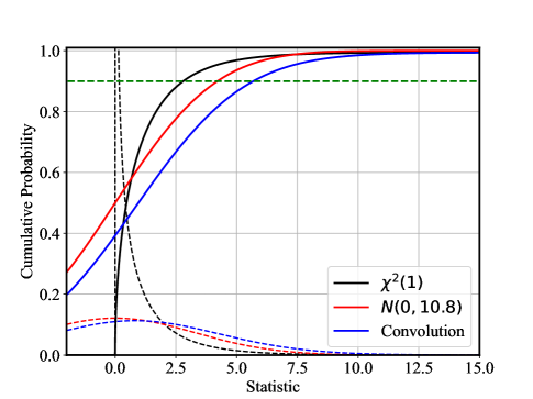
Figure 2: Distribution of the overdispersed $\chi^{2}$ distribution, resulting from the convolution of Equation 28, for $\nu=1$ degree of freedom of the $\chi^{2}$ distribution, and a value $\sigma=3.7$ for the standard deviation of a zero–mean Gaussian.

This $B(\nu,\sigma^{2})$ distribution is proposed as the distribution of choice for the $\Delta C$ statistic with $\nu$ degrees of freedom, in the presence of an intrinsic model variance that is modelled as a zero–mean Gaussian distribution with variance $\sigma^{2}$, according to (27). The parameter $\sigma=\hat{\sigma}_{\Delta C}$ represents the intrinsic standard deviation, with the meaning that the range $C_{\mathrm{min}}\pm\hat{\sigma}_{\Delta C}$ contains approximately 68% of the expected intrinsic variability of the $\Delta C$ statistic, as caused by the intrinsic model variance. This intrinsic ‘design’ standard deviation is calculated according to (26), where the details of the nested model component are taken into account. For example, a value of $\hat{\sigma}_{\Delta C}=1$ for a $\Delta C$ statistic with $\nu=1$ degree of freedom — e.g., for the test of a nested component with 1 additional free parameter — increases the usual 90% critical value from 2.7 to 3.1. A larger value of $\hat{\sigma}_{\Delta C}=5$ brings the critical value to 7.7, with the meaning that any measurement of the $\Delta C$ statistic between 2.7 and 7.7 remain statistically acceptable at the 90% confidence level, in the presence of such systematic error. It is thus clear that underestimating or neglectic systematic errors can lead to erroneous conclusions in the hypothesis testing of additional nested components.

The overdispersed $\chi^{2}$ distribution is also appropriate as a parent distribution for the $C_{\text{min}}$ statistic itself. In fact, as discussed in Sect. 3.1.1, the $Z=C_{\mathrm{min}}$ statistic in the presence of systematic errors is the sum of two independent variables, the first of which is $X\sim\chi^{2}(N-m)$. Therefore, the overdispersed $\chi^{2}$ distribution with parameters $\nu=M-n$ and $\sigma^{2}=\hat{\sigma}^{2}_{C}$ is the distribution of choice for the $C_{\text{min}}$ statistic in the presence of an intrinsic model variance $\hat{\sigma}^{2}_{C}$. When $\nu\gg 1$, as is the case for most regressions, this distribution asymptotically converges to a normal distribution with expectation $\nu$ and variance $2\nu+\hat{\sigma}^{2}_{C}$, further assuming the data are in the large–count regime. Therefore, for many applications in this regime it may be convenient to use the normal approximation for the $C_{\text{min}}$ statistic in the presence of systematic errors, as discussed in Sect. 3.1.1.

It is clear that the convolution in (28) leads to a distribution that will feature negative values, unlike in the case of a $\chi^{2}$ distribution, which is positive definite. This is especially the case when $\nu$ is a small number and $\sigma^{2}$ a large value for the intrinsic variance, when large intrinsic model fluctuation can lead to a $C$ statistic that becomes in fact lower than $C_{\text{min}}$. In practice, the interest is in hypothesis testing with one–sided confidence intervals for this overdispersed $\chi^{2}$ distribution, and therefore the negative tail, even when significant as in the case of Fig. 2, is not of direct interest to the data analyst.

Table 1: Critical values for the overdispersed $\chi^{2}(\nu)$ distribution, as a function of several representative values of the intrinsic variance ($\hat{\sigma}_{C}$), and for selected $p$–values. In parenthesis are the corresponding critical values for the standard $\chi^{2}(\nu)$ distribution.

$\hat{\sigma}_{C}$	$\nu=1$						$\nu=2$						$\nu=3$
	$p=0.9$		$p=0.99$		$p=0.999$		$p=0.9$		$p=0.99$		$p=0.999$		$p=0.9$		$p=0.99$		$p=0.999$
1.0	3.1	(2.7)	7.0	(6.6)	11.8	(10.8)	4.9	(4.6)	9.5	(9.2)	14.1	(13.8)	6.5	(6.3)	11.6	(11.3)	16.5	(16.3)
2.0	4.1	(2.7)	7.9	(6.6)	12.6	(10.8)	5.6	(4.6)	10.2	(9.2)	14.9	(13.8)	7.1	(6.3)	12.3	(11.3)	17.2	(16.3)
5.0	7.7	(2.7)	13.4	(6.6)	18.5	(10.8)	8.9	(4.6)	15.0	(9.2)	19.9	(13.8)	10.1	(6.3)	16.6	(11.3)	22.0	(16.3)
10.0	14.0	(2.7)	24.7	(6.6)	33.4	(10.8)	15.1	(4.6)	25.8	(9.2)	33.7	(13.8)	16.2	(6.3)	27.1	(11.3)	35.3	(16.3)
15.0	20.3	(2.7)	36.3	(6.6)	49.2	(10.8)	21.4	(4.6)	37.2	(9.2)	48.8	(13.8)	22.5	(6.3)	38.4	(11.3)	50.2	(16.3)
20.0	26.7	(2.7)	47.9	(6.6)	65.1	(10.8)	27.8	(4.6)	48.8	(9.2)	64.0	(13.8)	28.8	(6.3)	49.9	(11.3)	65.4	(16.3)

3.3 Domains of applicability for the asymptotic distributions

The choice to use asymptotic distributions for $C_{\text{min}}$ in (15) and (16), and for $\Delta C$ in (24) and (27), is motivated by the goal of obtaining an analytic representation of the distribution of the associated overdispersed statistics that account for the presence of systematic errors. The systematic errors are also modeled, for the same reason, with a simple normal distribution. It is clear that these assumptions are not necessary to implement the methods discussed in this paper. Specifically, the estimation of the intrinsic variance (see Sect. 3.1.2) can also be made using different distributions for the $X$ and $Y$ variables, representing respectively the $C_{\text{min}}$ statistic and the systematic error. However, in the absence of a simple analytical form for the distribution, the convolution needs to be carried out numerically, and therefore the simple result of (22) is no longer guaranteed to apply. Similarly, the convolution that defines the overdispersed $\chi^{2}$ distribution in (28) can be carried out between any two distributions, for example if the analyst decides to forgo the assumption of normality for the systematic error, as was done for example by Lee et al. (2011) and Xu et al. (2014) in the context of a different framework to address systematic errors.

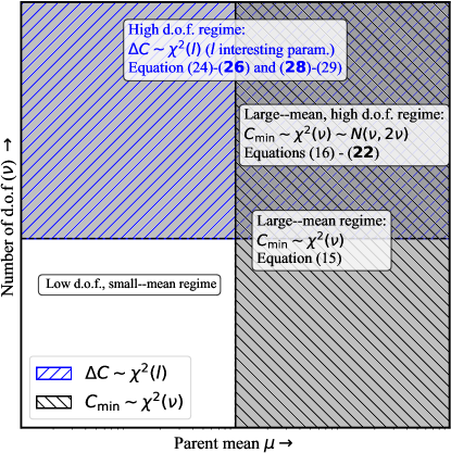
Figure 3: Domains of applicability of key results presented in this paper. Equations corresponding to the main results presented in this paper are shown in boldface. The domain of datasets with few datapoints and with small parent means (lower–left corner) is the portion of parameter space where the results of this paper do not generally apply.

The domains of applicability for the results presented in this section are summarized in Fig. 3. In particular, equation (22) applies in the large–mean regime, and for any number of degrees of freedom in $C_{\text{min}}$, while the overdispersed $\chi^{2}$ distribution presented in (28) applies for all values of the parent mean, thus even in the low–mean regime, but for a large number of degrees of freedom.

The boundaries between the domains are not sharp, and they can be estimated approximately as follows.

(a) In the high degree–of–freedom regime, the log–likelihood $\Delta C$ statistic is approximately $\chi^{2}$–distributed, when there is a large number of measurements. This result follows from the Wilks (1938) theorem, which shows that the log–likelihood is $\chi^{2}$–distributed to within a term of order $1/\sqrt{n}$ (see also Chapter 16 of Bonamente 2022). As a result, an approximate rule–of–thumb is that $\nu\geq 20$ or so might be sufficient to achieve a percent–level accuracy, and generally most astronomical datasets are in this regime.

(b) The large–mean regime where $C_{\text{min}}$ is $\chi^{2}$–distributed is essentially driven by the approximation of a Poisson distribution with a normal distribution of same mean and variance, which is well satisfied when $\mu\geq 10$ or so. This is shown for example by Kaastra (2017) and Bonamente (2020), who provide approximations for the mean and variance of the $C$ statistic in the low–mean regime with the aid of numerical calculations and simulations.

4 Application to the X–ray data of 1ES 1553+113

We illustrate the methods described in Sect. 3 to the XMM–Newton grating spectra of 1ES 1553+113, which are described in a separate paper (Spence et al., 2023). These data were used by Nicastro et al. (2018) to detect O VII absorption from the intervening warm–hot intergalactic medium, and they are representative of the data model discussed in this paper. The spectrum is shown in Figure 4, where the data points represent the total (integer) number of counts $y_{i}$ in a given bin, and the horizontal markers represents the best–fit model $\hat{\mu_{i}}$. Several wavelength ranges where excluded because of poor calibration, and several bins adjoining excluded ranges have a smaller size than the default 20 mÅ bin size that is used in the data reduction process, thus the lower number of counts.

For the purposes of this paper, the details of the continuum modelling are not important, and the main statistics of interest to the present analysis are summarized in Table 2. The methods of hypothesis testing and the determination of the systematic error only rely on the numbers presented in that table. For reference, the analysis is briefly summarized in the following. The model used to fit the data comprises a spline continuum with several free parameters in the 13–33 Å wavelength range, and additional components that model the local background. Specifically, the spline continuum was parameterized in 1 Å intervals, to each of which corresponds one free parameter. For these data, the background flux is $\sim 10$% of the source’s flux on average over the interesting wavelength range, and it has much smaller fluctuations that the source because it is collected from a larger area compared to that of the point source. The spectral analysis was conducted with the SPEX 3.0 fitting package (Kaastra et al., 1996), which uses the integral number of counts (source plus background) to calculate the $C$ statistic. A full description of the data and data analysis is provided in a companion paper (Spence et al., 2023), including an analysis of the background and its effects on the calculation of the fit statistics.

4.1 Hypothesis testing and the need for systematic errors

The method of hypothesis testing with the $C$–stat is described in detail in Kaastra (2017) and in Bonamente (2022). For this application, the method is simplified considerably by the large–$N$ and large–mean regime of these data, where the $C_{\text{min}}$ statistic is expected to be distributed like a $\chi^{2}(N-m)$ distribution, where $m$ is the number of free parameters in the fit. Given that a $\chi^{2}$ random variable with $\nu$ degrees of freedom has a mean of $\nu$ and a variance of $2\nu$, the measured value of the statistic needs to be compared with confidence intervals of this distribution.

For convenience, in the following the range $\nu\pm\sqrt{2\nu}$ is used to indicate the range within one standard deviation of the mean of a $\chi^{2}$ distribution with $\nu$ degrees of freedom. It is useful to point out that this range for $C_{\text{min}}$ is somewhat different from what is reported by the SPEX package, which instead assumes that the expectation of the fit statistic is equal to the sum of the $N$ expectations for each of the contributing terms of (3), asymptotically $N\pm\sqrt{2N}$ for large means, with no reference to the number of adjustable parameters (Kaastra, 2017). Although there is only a small difference between the two ranges in Table 2, the reader is referred to Sect. 16.3 of Bonamente (2022) and to Bonamente (2020), where the method of hypothesis testing with the $C$–stat is described in detail, including what is known concerning the reduction–of–degrees–of–freedom for the $C$–stat, based on a theorem of Wilks (1938). As already remarked earlier in the paper (see Sect. 3.1), the issue is also addressed in McCullagh (1986), who showed that the first–order approximation for the mean of $C_{\text{min}}$ is $N$, while a second–order approximation provides the $m$ correction, to yield an expectation of $\nu=N-m$. Accordingly, in this analysis we assume a reduction–of–degrees–of–freedom result for the $C$–stat, with a parent mean of $\nu$ for the $C_{\text{min}}$ statistic in the large–count limit.

Hypothesis testing is based on the $p$ value of the fit, defined as the probability that the measured statistic (in this cases $C_{\text{min}}$) has a value greater or equal than the measured value, under the hypothesis that the data are drawn from the parent model, i.e., the model under consideration is an accurate representation of the data. For the overall $C_{\text{min}}$=1862.7 statistic and its expectation based on the $\chi^{2}(N-m)$ asymptotic distribution reported in Table 2, the measured value falls at a value of $z=+7.1$ standard deviations from the parent mean under the null hypothesis of $1478\pm 54.4$, which corresponds to an infinitesimally small $p$–value. Similar conclusions apply to the two fit statistics for the RGS1 and RGS2 data considered separately. It is therefore clear that the measured fit statistics are not compatible with the null hypothesis.

This situation of a higher–than–expected fit statistic — be it the $C$–stat or $\chi^{2}$ — is quite common in X–ray astronomy. In cases where there are extended wavelength regions where the best–fit model is significantly above or below the data (of which there are numerous examples in the literature, such as Fig. 4 of Bonamente et al. 2003 for a different dataset), the best course of action is to deem the current model unacceptable, and thus discard it and try an alternative model. In this case, however, there are no systematic trends in the residuals, i.e., the best–fit model appears to be an overall reasonable approximation to the data. The analyst is thus presented with two alternative choices: (a) to discard this model, or (b) to investigate whether there may be additional sources of uncertainty that might have contributed to the mis–match between measured and expected value for the fit statistic. In this section we follow the latter approach, and use the method of Sect. 3 to estimate the amount of intrinsic variance in the model that brings the model to an acceptable degree of agreement with the data. This method assumes that there is no structure in the residuals, i.e., the additional variance in the data is somewhat uniformly distributed among all datapoints. When following this approach, the analyst must thus ensure that there is an analysis of the residuals that supports this assumption. For the data at hand, the analysis provided in Spence et al. (2023) indeed indicates that there is no significant structure in the residuals.

It is also useful to remark, at this point, that in the astrophysical literature it is common to report a reduced value for the fit statistic (typically the value of $\chi^{2}_{\text{red}}=\chi^{2}_{\text{min}}/\nu$), and deem the fit acceptable if such reduced value is ’close’ to one. A statistically more sound and quantitative approach is to report the $p$ value of the fit, as explained earlier in this section, since the proximity of a reduced value for $\chi^{2}$ or for the $C$ statistic is a strong function of the number of datapoints or of degrees of freedom. For the overall $C_{\text{min}}$ statistic and its expectation based on the $\chi^{2}(N-m)$ asymptotic distribution reported in Table 2, the $p$ value was found to be essentially zero, although the value of the reduce $C_{\text{min}}$ statistic is 1.29, and it may be erroneously deemed ‘close’ to unity.

Prior to the estimation of systematic errors according to the methods of Sect. 3, we use Equations 9 and 11 to estimate the overdispersion parameters in the data. For the NB1 parameterization, we estimate

$$\hat{\phi}=\begin{cases}1.58\pm 0.05\;\text{ for RGS1 data}\\ 1.35\pm 0.05\;\text{ for RGS2 data}\end{cases}$$ (30)

where the uncertainties are based on a simple error–propagation or delta method, assuming that the estimated mean values are known accurately. Given that $\hat{\phi}>1$, the estimate confirms the presence of an additional source of variance in the data. For the NB2 parameterization, we estimate

$$\hat{\alpha}=\begin{cases}1.5\pm 0.3\times 10^{-3}\;\text{ for RGS1 data}\\ 0.6\pm 0.2\times 10^{-3}\;\text{ for RGS2 data}\end{cases}$$ (31)

where the $\alpha$ parameter multiplies the square of the mean number of counts per bin, thus the lower absolute value compared with the NB1 model. As for the previous parameterization, the value $\hat{\alpha}>0$ indicated overdispersion. The $\hat{\phi}$ and $\hat{\alpha}$ parameters provide quantitative evidence for overdispersion in the data, relative to the best–fit model obtained with the usual Poisson log–likelihood. The parameters, however, do not address the effect of overdisperion or intrinsic model variance on the fit statistic, which is studied in the following using the methods presented in Sect. 3.

4.2 Estimate of systematic model uncertainty with the $C$–stat

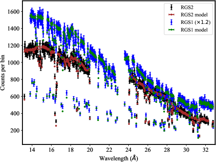
Figure 4: Left: XMM–Newton spectrum of the quasar 1ES 1553+113, which includes two independent spectra from the RGS1 and RGS2 cameras. For clarity, the RGS1 data was shifted by a factor of 1.2. Right: Zoom–in of the spectrum in a narrow wavelength interval, to illustrate the data and model. For each datapoint, the black dot represents the integer number of counts (source plus background), and the error bar is the Poisson error, which is not explicitly used for the $C$–stat.

Table 2: Fit statistics for the XMM–Newton spectrum of 1ES 1553+113

Statistic	Value	Notes
Combined RGS1 and RGS2 data
$C_{\text{min}}$	1862.7	($1861.8$ from Spence et al. 2023) ⋆
$\chi^{2}$	1730.6	(not used in the minimization)
$N$	1526	Number of data points
$m$	48	Number of free parameters
$f=N-m$	1478	Number of degrees of freedom
Expected $C$–stat	$1526.4\pm$ 55.3	As reported by SPEX
	$1478\pm 54.4$	According to the $\chi^{2}(N-m)$ approx.
RGS1 data
$C_{\text{min}}$	1023.5
$N_{1}$	801
$\chi^{2}$	1023.5
$m_{1}$	48	Resulting in $N_{1}-m_{1}=753$ d.o.f.
Expected $C$–stat	$753.0\pm 38.8$	According to the $\chi^{2}(N-m)$ approx.
RGS2 data
$C_{\text{min}}$	788.2
$N_{2}$	725
$\chi^{2}$	788.2
$m_{2}$	44	Data in 20–24 Å range ignored,
		resulting in $N_{2}-m_{2}=681$ d.o.f.
Expected $C$–stat	$681.0\pm 36.9$	According to the $\chi^{2}(N-m)$ approx.

4.2.1 Preliminary considerations

Given the values of the statistics reported in Table 2, it is reasonable to proceed independently with an analysis of the two XMM–Newton instruments. In so doing, this application also illustrates the determination of systematic errors from more than one independent dataset. First of all we point out that the model in use does not allow for a free normalization between the models applied to RGS1 and RGS2. We therefore begin the investigation for the origin of the poor fit statistic by repeating the same fit only to RGS1 and RGS2 data. From this exercise, we obtained statistically equivalent fits as the ones reported at the bottom of Table 2, which refers to the contributions to the statistic from the usual joint RGS1 plus RGS2 regression of Spence et al. (2023). We thus conclude that a cross–normalization error between the two instruments is not the origin for the poor $C_{\text{min}}$ value. We therefore proceed with the numbers in Table 2 as the basis for our estimate of the systematic error.

4.2.2 Determining the design value for the variance of $C_{\text{min}}$

The starting point is to determine a ‘design’ value for the intrinsic variance of the $C_{\text{min}}$ statistic required to bring agreement with the measured value. Qualitatively speaking, such value must bring agreement between the distribution function of the $C_{\text{min}}$ statistic and the measured value, currently at odds (e.g., RGS1 has a measured value of 1023.5 versus an expectation and standard deviation of $753.0\pm 38.8$). With $F_{C}$ the cumulative distribution function of the parent distribution of the $C_{\text{min}}$ statistic, one may require that the measured value of the statistic satisfies

$$F_{C}(C_{\text{min}})=1-p,$$ (32)

where $p$ is a high probablity, e.g., $p=0.9$ or 0.99. Eq. 32 means that the measured value $C_{\text{min}}$ is required to be the $p$ quantile, with a residual probability of just $1-p$ to exceed the measured value, according to the sampling distribution of the fit statistic. Equation 32 uses a single–sided rejection region of $C_{\text{min}}>C_{\text{crit}}$, as is customary for hypothesis testing with the $\chi^{2}$ distribution. In (32), $C_{\text{min}}$ is the actual measurement of the statistic with the data at hand. Given that the problem of intrinsic variance arises when the statistic is sufficiently large and in excess of its expectation, (32) is understood as featuring a measurement of the statistic at the boundary of the rejection region, i.e., $C_{\text{min}}=C_{\text{crit}}$.

When the $C_{\text{min}}$ statistic is normally distributed (which is the case for a large number of measurements and in the large–count limit, as is the case for this application), then (32) is equivalent to the familiar requirement that the measured value exceeds the mean by a predetermined number of standard deviations,

$$C_{\text{min}}=\text{E}[C_{\text{min}}]+\beta\times\sqrt{\text{Var}(C_{\text{min}})}$$ (33)

with $\beta=1.28$ or 2.33 for values of $p=0.9$ or 0.99. Equations 32 or 33 must be solved for the value of the intrinsic variancs $\hat{\sigma}^{2}_{C}$, with

$$\text{Var}(C_{\text{min}})=\sigma^{2}_{C}+\hat{\sigma}^{2}_{C}$$ (34)

and $\sigma^{2}_{C}$ indicating the parent variance of the statistic without accounting for the intrinsic model uncertainty. The design value for the intrinsic variance is immediately calculated from (32) (or (33) assuming Gaussian distribution for the fit statistic) and (34) as

$$\hat{\sigma}^{2}_{C}=\dfrac{\left(C_{\text{min}}-\text{E}[C_{\text{min}}]\right)^{2}}{\beta^{2}}-\sigma^{2}_{C}.$$ (35)

For the values of the statistics in Table 2 and with a choice of $\beta=2.33$ (corresponding to a 99% one–sided confidence level), Eq. 35 yields the following values of the intrinsic variance for the RGS1 and RGS2 data separately:

$$\begin{cases}\hat{\sigma}_{C,1}=&109.4,\;\text{ for a prediction of $753\pm 116$;}\\ \hat{\sigma}_{C,2}=&57.0,\;\text{ for a prediction of $681\pm 67.9$.}\\ \end{cases}$$ (36)

When these intrinsic variances are combined for the entire RGS1+RGS2 spectrum, they result in

$$\hat{\sigma}_{C}=123.4,\;\text{ for an overall prediction of $1478\pm 134.8$.}$$ (37)

Equations 36 and 37 are the sought–after estimates for the ‘design variances’ required for statistical agreement between the best–fit model and the data, according to the maximum–likelihood Poisson $C_{\text{min}}$ goodness of fit statistic. These design variances were added to the original ‘statistical’ variances of $C_{\text{min}}$ (i.e., the variances based on the Poisson counting statistics of the data) according the (34), to yield the overall variance of each statistic. Notice how the $z$-score of the overall $C_{\text{min}}$ statistic is now $z=2.85$, given the usual measurement of $C_{\text{min}}$=1862.7 and the revised expectation of $1478\pm 134.8$, corresponding to a one–sided null hypothesis probability to exceed the measured value of $p\simeq 0.002$.

4.2.3 The estimate of the intrinsic variance

With these design values for the intrinsic variance of the fit statistic, the use of (22) provides the values of the intrinsic model error. The average number of counts is respectively 728.6 for RGS1, 756.2 for RGS2, and 741.7 for the combined dataset. Accordingly, the method yields

$$\dfrac{\sigma_{\text{int},i}}{\hat{\mu_{i}}}=\begin{cases}0.072\,\text{ for RGS1}\\ 0.039\,\text{ for RGS2}\\ 0.058\,\text{ for combined RGS1 and RGS2}.\end{cases}$$ (38)

The interpretation of these numbers is that there is a level of systematic uncertainty in the best–fit models in the amount of respectively 7.2%, 3.9% and 5.8% in RGS1, RGS2 and for the combined data.

This method has therefore provided estimates of the intrinsic model variance based on simple analytical methods, for the individual RGS1 and RGS2 spectra and for the combined spectrum. These variances are estimated as fractional errors of the best–fit model in each bin according to (38), assuming that the relative systematic errors are uniform across the spectrum. It is necessary to compare these numbers with known systematic errors of the XMM–Newton instrument. Spence et al. (2023) shows that the typical systematic errors are of order of a few percent of the number of counts in a bin of the size used for this analysis (see also Marshall et al., 2021). The results of the analysis presented in this paper, with 4-7% fluctuations relative to the mean, is therefore consistent with the known level of systematic errors in the instrument.

Finally, it is useful to compare the values of estimated overdispersion parameter $\hat{\phi}$ from (30) with the intrinsic model variance in (38). The overdisperion parameter $\hat{\phi}=1.3-1.6$ models the additional variance in each measurement, with a value of $\phi=1.0$ representing a variance equal to the mean. The square root of the variance $\omega_{i}=\hat{\phi}\,\mu_{i}$ (or $\omega_{i}=\mu_{i}+\alpha\mu_{i}^{2}$ for the alternative parameterization) needs to be divided by the mean number of counts in the bin ($\mu_{i}$) in order to assess the additional level of fractional systematic errors in the data implied by the extra variance. For a typical count rate in these data of several hundred counts per bin, the estimated values of $\hat{\phi}$ and $\hat{\alpha}$ yield fractional fluctuations that are a few percentage points larger than the case of $\phi=1$, in general accord with the percent–level intrinsic model variance estimated in (38).

4.3 Systematic errors in the data with the $\chi^{2}$ statistic and other considerations

Given that the analysis of Sect. 4.2 indicates an intrinsic model uncertainty of order $\sim 5$%, it is natural to ask the question of how such uncertainty, if applied to the data instead, would affect the $\chi^{2}$ statistic. The reason to pursue this comparison is that of providing a consistency check with a more traditional, albeit less accurate, method of assessing systematic errors in the data in the presence of an unacceptable fit statistic.

To this end, we apply the average intrinsic errors of (38) to each data point, and add them in quadrature to the usual Poisson errors. With this change in the data errors, the $\chi^{2}$ statistics are modified to

$$\chi^{2}=\begin{cases}874.8\,\text{ for RGS1 }(\Delta\chi^{2}=-68.5)\\ 626.1\,\text{ for RGS2 }(\Delta\chi^{2}=-101.82)\\ 1500.9\,\text{for RGS1+RGS2 }(\Delta\chi^{2}=-170.4).\end{cases}$$

with respect to the values of Table 2. The main result is that a systematic error added to the data in the amount of 6.5% results in a decrease of $\Delta\chi^{2}=-170.4$, bringing the statistic in closer agreement with its expectation, for the given number of degrees of freedom ($\nu=1478$). This exercise therefore indicates that the values of the intrinsic model variance estimated from the Poisson data and the $C$–stat with the novel method described in Sec. 4.2 are reasonable, in that a systematic error of the same magnitude applied to the data and to the $\chi^{2}$ statistics bring this statistic closer to its expectation, in a manner similar to the change in the $C_{\text{min}}$ statistic using the intrinsic model variance.

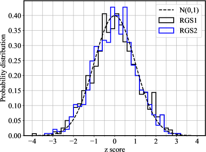
Figure 5: Distribution of $z$–scores for the RGS1 and RGS2 data. The mean and standard deviation of the two samples are respectively 0.00 and 1.08 for the RGS1 z–scores, and -0.01 and 1.04 for the RGS2 z–scores.

It is also instructive to plot the probability distribution of the $z$–scores associated with the residuals from the best fit, using the usual Poisson counts as the data variance. These distributions, shown in Fig. 5, do not show any significant departure from the standard normal distribution, which is the expected distribution under the null hypothesis. This observation is also confirmed by a Kolmogorov–Smirnov test (Kolmogorov, 1933), which is an empirical distribution function (EDF) test that uses unbinned data. The one–sample Kolmogorov–Smirnov test statistics are $D_{N}=0.033$ and 0.018 respectively for the RGS1 and RGS2 data, with corresponding $p$–values of respectively 0.33 and 0.97, indicating an excellent agreement between the data and the parent model.  The Kolmogorov–Smirnov test is therefore not sensitive for the detection of systematic errors at the level of a few percent, i.e., at the level present in the data of this case study. The Anderson–Darling EDF statistic (Anderson & Darling, 1952; Stephens, 1974) for the test of normality of the distributions has values of $A^{2}=0.32$ and 0.21 respectively for the RGS1 and RGS2 data, with a corresponding 99% critical value of 1.09 for both data, indicating that the null hypothesis of normally distributed data cannot be rejected. Therefore, similar to the one–sample Kolmogorov–Smirnov test, the Anderson–Darling test cannot find deviations from normality in the z–scores. 

4.4 Effect of intrinsic errors on a nested component with the $\Delta C$ statistic

Equation 26 provides the means to estimate the uncertainty in the $\Delta C$ statistic due to the intrinsic model variance. For the case study with the 1ES 1553+113 XMM–Newton data, the relevant statistics are reported in Table 3, reproduced from Spence et al. (2023). The regressions used for the detection of a nested line component are now performed in narrow bands of $\pm 1$ Å around the expected line features, instead of a broad–band fit (as for the results of Table 2). For the data of Table 3, the baseline model is composed by a simple power–law model, supplemented by a Gaussian line model (line in SPEX). The line models provide a deviation from the smooth continuum at the level of a few percent, and therefore it is useful to determine how an intrinsic error at a similar level affects the significance of detection of these features. An illustration of the data leading to the reults of Table 3 is provided in Figure 4 of Spence et al. (2023).

Table 3: $\Delta C$ statistics from the fit to a power–law model plus a Gaussian line feature for the XMM–Newton data of 1ES 1553+113, reproduced from Spence et al. (2023). The ‘$p$–value’ columns correspond to the usual $p$ values of the regression, and the ’$P$ value’ columns correspond to the $p$–value with the inclusion of uncertainties associated with the blind search of lines at an unknown redshift.

Target line	$\Delta C$	$\nu$	$p$–value		$P$ value with redshift trials
			(no sys. error)	overdispersed $\chi^{2}$ distr.	(no sys. error)	overdispersed $\chi^{2}$ distr.
O VII $z=0.1876$	6.6	1	0.010	0.066	–	–
O VII $z=0.4339$	29.9	2	$3.2\times 10^{-7}$	$2.6\times 10^{-5}$	$4.1\times 10^{-5}$	$3.3\times 10^{-3}$
O VII $z=0.3551$	8.2	2	0.017	0.880	–

The largest uncertainty in the use of (26) is the number $n$ of independent datapoints in the sum. In the case of an absorption line–like model such as the Gaussian profile of line, a simple method to determine the number of independent data points is by calculating the equivalent width of the absorption–line feature. In all cases, the equivalent width is smaller than the instrument’s resolution, and therefore a simple estimate is $n=1$, meaning that the model affects just one datapoint, also leading to a conservative (i.e., the smallest possible) estimate of the intrinsic variance. With a characteristic number of counts of respectively 800, 500 and 400 per bin for the three lines, and an intrinsic model error of $\sigma_{\text{int,i}}/\hat{\mu}_{i}=0.058$ as estimated in Sect. 4.2.3, (26) leads to an estimate of

$$\hat{\sigma}^{2}_{\Delta C}=\begin{cases}\begin{aligned} 10.8\;&\text{ for line 1}\\ 6.7\;&\text{ for line 2}\\ 5.4\;&\text{ for line 3}.\\ \end{aligned}\end{cases}$$ (39)

Following the modified $\chi^{2}$ distribution for the $\Delta C$ statistic in the presence of intrinsic errors described in Sect. 3.2, it is now possible to determine whether the three lines in Table 3 remain statistically significant, after accounting for the effect of systematic errors. The results are reported in the ‘$p$–value’ columns of Table 3.

The statistical significance of the first line is reduced from a $p$–value of 1% to $\sim 7\%$. It is therefore possible to conclude that, if the additional variance of the data relative to the best–fit models of Table 2 is interpreted as an additional source of systematic error, as the methodology presented in this paper posits, then the absorption line at $z=0.1876$ is likely caused by a statistical fluctuation, and unlikely to be a genuine celestial signal. In this paper, it is not appropriate to further comment on the astrophysical significance of this putative absorption line, since the main aim of this report is to establish a method of analysis for systematic errors. The conclusion is thus that sources of systematic errors in Poisson data such as the spectra analyzed in Spence et al. (2023) can be easily addressed, and that their impact can be significant.

The second line, originally reported by Nicastro et al. (2018), is also reduced in significance by factor of nearly $\sim 100$. For this absorption line, it is necessary to consider the fact that its redshift was identified serendipitously, thus the additional degree of freedom in the analysis (i.e., the center wavelength of the absorption line). For such serendipitous sources, Kaastra et al. (2006) and Bonamente (2019) describe a method to address the several independent opportunities to detect a fluctuations, known as redshift trials. Given the large number of independent opportunities to detect a random fluctuations, estimated in Spence et al. (2023) to be of order $N\simeq 100$, the method described in Bonamente (2020) results in corrected $p$–values that are reported in the right–most columns of Table 2 . Using the revised $p$–value from the overdispersed $\chi^{2}$ distribution, the redshift trials–corrected $P$ value is now approximately 0.003, which corresponds approximately to a $\pm 3\sigma$ two–sided confidence level for a normal distribution. It is therefore clear that even a seemingly ‘strong’ detection of a nested model component ($\Delta C=29.9$ for 2 degrees of freedom) can in fact become far less significant due to the effect of percent–level systematic errors.

The same analysis is not warranted for the third line, given that it is not statistically significant even without accounting for the intrinsic variance (probability of 88% according to the overdispersed $\chi^{2}$ distribution). The redshift trials correction does not apply to the first line, given that its central wavelength was fixed at its known value, and therefore it features no redshift trials.

4.5 Summary of steps for a typical implementation

In this section we provide a short summary of the steps for a typical implementation of the methods presented in this paper, with the goal of estimating the systematic errors in Poisson count data from the maximum–regression of a parametric model with the $C_{\text{min}}$ statistic, and for the assessment of the significance of a nested model component with the $\Delta C$ statistic.

1. Determination of the design variance $\hat{\sigma}^{2}_{C}$ from (35), where $C_{\text{min}}$ is the measured statistic from the parametric regression, with $\nu$ degrees of freedom. This step requires the choice of a value of $\beta$ for the agreement between the measured statistic and its parent distribution. The expectation of the $C_{\text{min}}$ statistic is $\nu$ in the large count regime, and a discussion for the low–count regime was provided in Sect. 4.1.

2. The fractional systematic error $\sigma_{\text{int,i}}/\hat{\mu_{i}}$ is estimated from (22), where $N$ is the number of independent Poisson datapoints, and $\hat{\mu_{i}}$ is the best–fit model for the i–th datapoint. This number represents the fractional uncertainty associated to the best–fit model of each datapoint.

3. When the significance of a nested component needs to be assessed, the first step is the determination or estimation of the number $n$ of bins where the nested model is present, and then the variance $\hat{\sigma}^{2}_{\Delta C}$ estimated according to (26).

4. The $\Delta C$ associated to the additional nested component with $\nu=l$ additional parameters is then compared to the parent overdispered $\chi^{2}$ distribution $B(l,\hat{\sigma}^{2}_{\Delta C})$ defined in (28). Typically this is achieved via numerical solution of the equation (29) which gives the $p$–value associated with the $\Delta C$ statistic.

All these steps require minimal computational effort, given that most results are elementary analytical formulas, and the numerical integration of the overdispersed $\chi^{2}$ distribution is an elementary task, given its simple unimodal behavior.

5 Discussion and conclusions

This paper has presented a simple quantitative method to estimate systematic uncertainties in the maximum–likelihood fit of Poisson count data to a parametric model, using the Cash statistic. This situation is of common occurrence in the analysis of X–ray spectra from astronomical sources of the type presented in the case study of 1ES 1553+113 (Spence et al., 2023). This sources is a bright quasar where the goodness of fit statistic across an extended wavelength range is formally unacceptable, yet the data do not have significant and systematic deviations from the best–fit model. In such cases, the data analyst is faced with the choice to either reject the model altogether, or to determine the presence of additional source of error that are not present in the Poisson–distributed data. When the analyst determines that it is reasonable to pursue the latter avenue, the method developed in Sect. 3 leading to the main result presented in Eq. 22 provides a simple quantitative method to estimate an intrinsic variance present in the model that renders the data and best–fit model consistent at a predetermined $p$–value. In the case of the 1ES 1553+113 data presented in this paper and in Spence et al. (2023), we find that the higher–than–expected $C$–stat for the fit to a complex parametric model can be naturally explained with the presence of a $\sim 5$% systematic uncertainty in the best–fit model. The method does away entirely with the more commonly used $\chi^{2}$ statistic, which is not appropriate for the regression of integer–count and Poisson distributed data, such as the majority of astronomical X–ray spectra (as shown in, e.g., Humphrey et al., 2009; Bonamente, 2020).

A key application of the intrinsic model variance is through the effect it has on the $\Delta C$ statistic, which is a likelihood–ratio statistic that is commonly used to test for the significance of an additional nested component (e.g. Protassov et al., 2002). Following the methods described in Sect. 3.2, it was shown that the intrinsic model variance leads to an additional contribution to the $\Delta C$ statistic that can be modelled as a normal distribution with zero mean and a design variance $\hat{\sigma}^{2}_{\Delta C}$. This additional distribution is to be added to the usual $\chi^{2}(\nu)$ distribution, which represents the Poisson variability in the $\Delta C$ statistic from the nested model component with $\nu=l$ free parameters. This leads to the introduction of the overdispersed $\chi^{2}$ distribution that replaces the usual $\chi^{2}(\nu)$ distribution for the test of the additional nested component. This newly introduced distribution, which is the convolution of the two contributing probability distributions $\chi^{2}(\nu)$ and $N(0,\hat{\sigma}^{2}_{\Delta C})$, is the parent distribution for the usual $\Delta C$ statistic in the presence of systematic errors, under the null hypothesis that the nested component is not present, thus leading to a simple method of hypothesis testing for the nested component. With the choice of attributing the additional variability caused by systematic effects to the model, as opposed to the data, the calculation of the $\Delta C$ statistic itself remains unchanged, and the hypothesis testing for the nested component thus only requires the calculation of critical or $p$–values for this new overdispersed $\chi^{2}$ distribution, e.g. of the type reported in Table 3.2.4.

In the case study of the 1ES 1553+113 source, the $\Delta C$ statistic was used to test for the presence of additional absorption line components. The $\sim 5\%$ systematic error in the best–fit model results in a an additional variance in the $\Delta C$ distribution, and in a lower level of significance for the detection of the lines, as reported in Table 3. For example, the first line under consideration, which was identified in Spence et al. (2023) as a possible O VII resonance line at $z=0.1876$, would have its significance reduced from a 99% level to a 93% level (i.e., $p$–value increasing from 0.01 to 0.07). The other absorption line that was reported by Spence et al. (2023), and which was previously discovered by Nicastro et al. (2018), has its significance of detection also greatly reduced by the effect of the intrinsic model variance (see second line in Table 3), yet it remains above the 99% confidence level ($p$–value of 0.003). The use of systematic errors in likelihood–ratio statistics (such as $\Delta C$ or $\Delta\chi^{2}$) for the detection of additional nested components has therefore the potential to affect the astrophysical inference from count data, such as from high–energy spectra of the type investigated in this case study. This is especially important in fields such as the detection of X–ray absorption lines from the WHIM, where the combination of a faint astrophysical signal and limited resolution in the intruments have combined to produce a number of detections (e.g. Ahoranta et al., 2021, 2020; Nevalainen et al., 2019; Kovács et al., 2019; Bonamente et al., 2016; Ren et al., 2014; Fang et al., 2010; Nicastro et al., 2005; Fang et al., 2007, 2002) that have the potential to be affected by such systematic errors.

The Cash statistic was developed in response to the advent of new integer–count astronomical X–ray data, as the maximum–likelihood fit statistic of choice for Poisson data (e.g., Cash, 1976, 1979). This statistic is often referred to as the Poisson log–likelihood deviance in other fields of statistics (e.g. Cameron & Trivedi, 2013). Recently, the author also developed a new semi–analytical method to obtain the best–fit parameters for the linear regression of count data, a problem that was previously only solved numerically (Bonamente & Spence, 2022). The typical implementation of the methods described in this paper are outlined in Sect. 4.5, and it is expected to be straightforward for most applications. Given that the $C$–stat is usually the appropriate fit statistic for the maximum–likelihood analysis of these data, the method presented in this paper therefore provides an additional tool for the X–ray astronomer (or any other count–data analyst) who wishes to use the Cash statistic for their data analysis.

Data Availability

The XMM–Newton X–ray data associated with the 1ES 1553+113 source are available via heasarc.gsfc.nasa.gov/cgi-bin/W3Browse. Processed data such as spectra can be obtained from the author upon request. Numerical routines in python to implement and reproduce the key results of this paper, namely the overdispersed $\chi^{2}$ distribution (28) and the critical values of the distribution in Table 3.2.4, are available at https://github.com/bonamem/overdispersedChi2.

References

- Ahoranta et al. (2021) Ahoranta J., Finoguenov A., Bonamente M., Tilton E., Wijers N., Muzahid S., Schaye J., 2021, A&A, 656, A107
- Ahoranta et al. (2020) Ahoranta J. et al., 2020, A&A, 634, A106
- Anderson & Darling (1952) Anderson T. W., Darling D. A., 1952, The Annals of Mathematical Statistics, 23, 193
- Arnaud (1996) Arnaud K. A., 1996, in Astr. Data Analysis Software and Systems V, Jacoby G. H., Barnes J., eds., Vol. 101, p. 17
- Baker & Cousins (1984) Baker S., Cousins R. D., 1984, Nuclear Instruments and Methods in Physics Research, 221, 437
- Bevington & Robinson (2003) Bevington P. R., Robinson D. K., 2003, Data reduction and error analysis for the physical sciences. McGraw Hill, Third Edition
- Bishop et al. (1975) Bishop Y., Fienberg S., Holland P., 1975, Discrete Multivariate Analysis: Theory and Practice : Yvonne M.M. Bishop, Stephen E. Fienberg and Paul W. Holland. Massachusetts Institute of Technology Press
- Bonamente (2019) Bonamente M., 2019, Journal of Applied Statistics, 46, 1129
- Bonamente (2020) Bonamente M., 2020, Journal of Applied Statistics, 47, 2044
- Bonamente (2022) Bonamente M., 2022, Statistics and Analysis of Scientific Data. Springer, Graduate Texts in Physics, Third Edition
- Bonamente et al. (2003) Bonamente M., Joy M. K., Lieu R., 2003, ApJ, 585, 722
- Bonamente et al. (2016) Bonamente M., Nevalainen J., Tilton E., Liivamägi J., Tempel E., Heinämäki P., Fang T., 2016, MNRAS, 457, 4236
- Bonamente & Spence (2022) Bonamente M., Spence D., 2022, Journal of Applied Statistics, 49, 522
- Cameron & Trivedi (1986) Cameron A. C., Trivedi P. K., 1986, Journal of Applied Econometrics, 1, 29
- Cameron & Trivedi (2013) Cameron C., Trivedi P., 2013, Regression Analysis of Count Data (Second Ed.). Cambridge University Press
- Cash (1976) Cash W., 1976, A&A, 52, 307
- Cash (1979) Cash W., 1979, ApJ, 228, 939
- Consul & Jain (1973) Consul P. C., Jain G. C., 1973, Technometrics, 15, 791
- Conway & Maxwell (1962) Conway T. R., Maxwell W. L., 1962, Journal of Industrial Engineering, 12, 132
- Cramer (1946) Cramer H., 1946, Mathematical Methods of Statistics. Princeton University Press, Princeton
- Dean & Lawless (1989) Dean C., Lawless J. F., 1989, Journal of the American Statistical Association, 84, 467
- Dean (1992) Dean C. B., 1992, Journal of the American Statistical Association, 87, 451
- Famoye (1993) Famoye F., 1993, Communications in Statistics - Theory and Methods, 22, 1335
- Fang et al. (2010) Fang T., Buote D. A., Humphrey P. J., Canizares C. R., Zappacosta L., Maiolino R., Tagliaferri G., Gastaldello F., 2010, ApJ, 714, 1715
- Fang et al. (2007) Fang T., Canizares C. R., Yao Y., 2007, ApJ, 670, 992
- Fang et al. (2002) Fang T., Marshall H. L., Lee J. C., Davis D. S., Canizares C. R., 2002, ApJ, 572, L127
- Fisher (1922) Fisher R., 1922, Journal of the Royal Statistical Society, 85, 87
- Fisher (1934) Fisher R., 1934, Statistical Methods for Research Workers, Fifth Ed. Oliver and Boyd, Edinburgh
- Giacconi et al. (1971) Giacconi R., Kellogg E., Gorenstein P., Gursky H., Tananbaum H., 1971, ApJ, 165, L27
- Gourieroux et al. (1984a) Gourieroux C., Monfort A., Trognon A., 1984a, Econometrica, 52, 701
- Gourieroux et al. (1984b) Gourieroux C., Monfort A., Trognon A., 1984b, Econometrica, 52, 681
- Greenwood & Nikulin (1996) Greenwood P., Nikulin M., 1996, A Guide to Chi-Squared Testing. Wiley
- Hilbe (2011) Hilbe J. M., 2011, Negative Binomial Regression, 2nd edn. Cambridge University Press
- Hilbe (2014) Hilbe J. M., 2014, Modeling Count Data. Cambridge University Press
- Humphrey et al. (2009) Humphrey P. J., Liu W., Buote D. A., 2009, ApJ, 693, 822
- Kaastra (2017) Kaastra J. S., 2017, Astronomy and Astrophysics, 605, A51
- Kaastra et al. (1996) Kaastra J. S., Mewe R., Nieuwenhuijzen H., 1996, in UV and X-ray Spectroscopy of Astrophysical and Laboratory Plasmas, Yamashita K., Watanabe T., eds., pp. 411–414
- Kaastra et al. (2006) Kaastra J. S., Werner N., Herder J. W. A. d., Paerels F. B. S., de Plaa J., Rasmussen A. P., de Vries C. P., 2006, ApJ, 652, 189
- Kolmogorov (1933) Kolmogorov A., 1933, Giornale dell’ Istituto Italiano degli Attuari, 4, 1
- Kovács et al. (2019) Kovács O. E., Bogdán Á., Smith R. K., Kraft R. P., Forman W. R., 2019, ApJ, 872, 83
- Lampton et al. (1976) Lampton M., Margon B., Bowyer S., 1976, ApJ, 208, 177
- Lee et al. (2011) Lee H. et al., 2011, ApJ, 731, 126
- Marshall et al. (2021) Marshall H. L. et al., 2021, AJ, 162, 254
- McCullagh (1984) McCullagh P., 1984, Biometrika, 71, 461
- McCullagh (1986) McCullagh P., 1986, Journal of the American Statistical Association, 81, 104
- McCullagh & Nelder (1989) McCullagh P., Nelder J., 1989, Generalized Linear Models. Chapman & Hall/CRC, Second Edition
- Nevalainen et al. (2019) Nevalainen J. et al., 2019, A&A, 621, A88
- Nicastro et al. (2018) Nicastro F. et al., 2018, Nature, 558, 406
- Nicastro et al. (2005) Nicastro F. et al., 2005, ApJ, 629, 700
- Protassov et al. (2002) Protassov R., van Dyk D. A., Connors A., Kashyap V. L., Siemiginowska A., 2002, ApJ, 571, 545
- Ren et al. (2014) Ren B., Fang T., Buote D. A., 2014, ApJ, 782, L6
- Rothschild et al. (1979) Rothschild R. et al., 1979, Space Science Instrumentation, 4, 269
- Sellers & Shmueli (2010) Sellers K. F., Shmueli G., 2010, The Annals of Applied Statistics, 4, 943
- Shmueli et al. (2005) Shmueli G., Minka T. P., Kadane J. B., Borle S., Boatwright P., 2005, Journal of the Royal Statistical Society. Series C (Applied Statistics), 54, 127
- Spence et al. (2023) Spence D., Bonamente M., Nevalainen J., Tuominen T., Ahoranta J., Liu W., Wijers N., 2023, MNRAS submitted, 0
- Stephens (1974) Stephens M. A., 1974, Journal of the American Statistical Association, 69, 730
- Wasserstein & Lazar (2016) Wasserstein R. L., Lazar N. A., 2016, The American Statistician, 70, 129
- Wilks (1938) Wilks S. S., 1938, Ann. Math. Statist., 9, 60
- Xu et al. (2014) Xu J. et al., 2014, ApJ, 794, 97