A NICER look at the jet-like corona of MAXI J1535$-$571 through type-B quasi-periodic oscillations

Abstract

MAXI J1535$-$571 is a black-hole X-ray binary that in 2017 exhibited a very bright outburst which reached a peak flux of up to 5 Crab in the 2–20 keV band. Given the high flux, several X-ray space observatories obtained unprecedented high signal-to-noise data of key parts of the outburst. In our previous paper we studied the corona of MAXI J1535$-$571 in the hard-intermediate state (HIMS) with Insight-HXMT. In this paper we focus on the study of the corona in the soft-intermediate state (SIMS) through the spectral-timing analysis of 26 NICER detections of the type-B quasi-periodic oscillations (QPOs). From simultaneous fits of the energy, rms and lag spectra of these QPOs with our time-dependent Comptonization model, we find that in the SIMS the corona size is $\sim$ 6500 km and vertically extended. We detect a narrow iron line in the energy spectra, which we interpret to be due to the illumination of the outer part of the accretion disk by this large corona. We follow the evolution of the corona and the radio jet during the HIMS-SIMS transition, and find that the jet flux peaks after the time when the corona extends to its maximum vertical size. The jet flux starts to decay after the corona contracts vertically towards the black hole. This behavior points to a connection between the X-ray corona and the radio jet similar to that seen in other sources.

1 Introduction

Black-hole low-mass X-ray binaries (BH LMXBs) consist of a stellar-mass black hole with a low-mass companion star overflowing its Roche lobe, forming an accretion disk (see Belloni et al., 2011; Kalemci et al., 2022, for reviews). During an outburst, a black-hole X-ray transient traces an anticlockwise ‘q’ path in the hardness-intensity diagram (HID; Homan & Belloni, 2005; Belloni et al., 2005), during which the proportion of the thermal and Comptonized components changes leading to several well-defined spectral states (Belloni et al., 2005). The accretion disk emits thermal emission in the soft X-ray band with the disk spectrum peaking at around 0.2–2.0 keV; a fraction of the soft disk photons are Compton up-scattered in the corona, forming a power-law like component in the energy spectrum in the hard X-ray band up to 100 keV (for reviews, see Done et al., 2007; Gilfanov, 2010). When the outburst starts, the X-ray luminosity of the source increases by several orders of magnitude compared to the quiescent state and the source enters the low-hard state (LHS) with a dominant hard Comptonized component and a relatively weak thermal disk component in the X-ray spectrum (e.g. Sharma et al., 2018; Wang-Ji et al., 2018). As the mass accretion rate increases, the source becomes brighter and quickly goes into the hard-intermediate state (HIMS), the soft-intermediate state (SIMS), the high-soft state (HSS), and sometimes an anomalous state at the highest luminosity (e.g. Méndez & van der Klis, 1997; Belloni et al., 2005; Belloni, 2010; Motta et al., 2012). From the LHS to the HSS, the truncated disk moves closer to the innermost circular stable orbit (ISCO) around the black hole (Esin et al. 1997; but see Reis et al. 2008; Wang-Ji et al. 2018 and Miller et al. 2018 for a different interpretation) and the thermal component becomes dominant, while the spectrum of the hard component becomes steeper and weaker (e.g. Sharma et al., 2018; Dong et al., 2022). With the gradual decay of the mass accretion rate, the source evolves back to the LHS and finally returns to the quiescent state. In some so-called failed-transition outbursts the source stays in the LHS and HIMS and never enters the SIMS (Alabarta et al., 2021).

The Comptonized photons in the corona can impinge back onto the accretion disk, resulting in the reprocessing and Compton back-scattering of the hard photons, which leads to a relativistic reflection component (Fabian et al., 1989; Bambi et al., 2021). The reflection spectrum includes characteristic X-ray emission lines among which the most prominent is the iron $K_{\alpha}$ line around 6.4–7.0 keV and the Compton hump around 20 keV (García et al., 2014). Recent studies have also modeled the relativistic reflection considering the incident photons coming from a hot blackbody or a returning reflection spectrum due to the strong gravitational bending (e.g. Connors et al., 2020; García et al., 2022b; Dauser et al., 2022). A relativistic reflection component can appear through the spectral evolution from the LHS to the HSS (e.g. Wang-Ji et al., 2018; Connors et al., 2020; Dong et al., 2022).

The X-ray light curves of black-hole binaries (BHBs) show variability on time scales from milliseconds to years (see Ingram & Motta, 2019, for a recent review). In the Fourier domain, the power density spectrum (PDS) of the X-ray light curve shows different kinds of variability, e.g. broadband noise and narrow peaks called quasi-periodic oscillations (QPOs; Van der Klis, 1989; Nowak, 2000; Belloni et al., 2002). The QPOs observed in BHBs are classified as low-frequency QPOs (LFQPOs), with central frequencies ranging from mHz to $\sim$ 30 Hz, and high-frequency QPOs (HFQPOs), with central frequencies $\gtrsim$ 60 Hz (Belloni & Stella, 2014). Depending on the shape of the broadband noise, the fractional root-mean-square amplitude (hereafter rms), the phase lags of the QPOs and the spectral state of the source, LFQPOs are divided into three classes, namely type A, B, and C (Remillard et al., 2002; Casella et al., 2004; Casella et al., 2005). Type-C QPOs generally appear in the hard states (both LHS and HIMS) with central frequency in the $\sim$ 0.01–30 Hz range, high rms (up to 20%), strong band-limited noise, and usually second and sub harmonics. Type-B QPOs only appear in the SIMS (Belloni & Motta, 2016), with central frequency below $\sim$ 6 Hz, low rms ($\lesssim 5\%$), weak red noise, and sometimes the second and sub harmonics. Type-A QPOs, which are rarely detected, appear in the SIMS and HSS, with central frequencies in the $\sim$ 6–8 Hz range, very weak rms and no harmonics. In the short-lived SIMS, fast transitions are sometimes observed between the type-B and either other types of QPOs or the disappearance of QPO (e.g. Casella et al., 2004; Zhang et al., 2021).

The Fourier cross spectrum of two simultaneous light curves in different energy bands (subject and reference band) can be used to compute the phase lags as a function of Fourier frequency. It is common to report lags of the signals identified in the PDS extending over a given frequency range, e.g. the broadband noise and the QPOs (Nowak et al., 1999). Hard (positive) lags (Miyamoto et al., 1988) can be produced by propagation of fluctuations of the mass accretion from the outer part towards the inner part of the disk and the corona (e.g. Arévalo & Uttley, 2006; Ingram & van der Klis, 2013). Soft (negative) lags can be due to reverberation or thermalization of hard photons when the corona photons impinge back onto the accretion disk (e.g. Uttley et al., 2014; Karpouzas et al., 2020).

Apart from the X-ray emission, BHBs radio emission from a jet is sometimes prominent, and can be classified into two types depending on the radio spectral index and the morphology of the jet: a small-scale, optically thick, compact jet and an extended, optically thin, transient jet (for a review, see Fender, 2006). The relation between the spectral states and the radio emission indicates the existence of an accretion-ejection coupling. In the LHS and the HIMS, a compact jet is observed, while during the state transition from the HIMS to the SIMS, the compact jet can be quenched for a few days (Fender et al., 2004). In the SIMS, there is no longer a compact jet but a bright transient jet appears with observable discrete relativistic ejecta, while in the HSS, the jet disappears (e.g. Mirabel & Rodríguez, 1994; Corbel et al., 2004; Ingram, 2019). Time variability in the radio band sometimes appears, but much less often than in the X-ray band (e.g. Tetarenko et al., 2019, 2021). Type-B QPOs in the X-ray band are usually thought to be connected to the relativistic transient jet but the exact mechanisms that explain the connection are still unknown (e.g. Fender et al., 2009; Homan et al., 2020; García et al., 2021).

There are still many open questions regarding the the disk-corona-jet evolution, for instance, the disk truncation during the evolution of the black hole transients (Esin et al., 1997), the nature of the corona (the inner hot flow, disk sandwich, or the base of the jet; Galeev et al., 1979; Haardt & Maraschi, 1991; Markoff et al., 2005), and the geometry of the corona and its typical size (Martocchia & Matt, 1996; Lee & Miller, 1998). The geometry of the corona and its connection with the disk and the jet are still to be understood. A universal radio–X-ray correlation in the LHS provides evidence that the corona can be related to the radio jet (e.g. Gallo et al., 2003; Fender et al., 2004). Using data of GRS 1915+105, Méndez et al. (2022) proposed that (part of) the spread in the radio–X-ray correlation (Gallo et al., 2012) could be due to changes of the corona temperature. Studies of the spectral energy distribution (SED) from the radio to the X-ray band shows that the corona emission can originate from a shock acceleration region of tens of gravitational radii ($R_{g}$) as the jet base (Markoff et al., 2001; Connors et al., 2019; Cao et al., 2022). The spectral analysis of the reflection component in MAXI J1820+070 suggests that the corona outflows with a higher relativistic velocity as it is closer to the black hole (You et al., 2021). Through X-ray variability studies, the size of the corona shows a continuous evolution during the outburst that could be related to the change of the radio jet emission, suggesting a disk-corona-jet connection (Kara et al., 2019; Wang et al., 2021; Méndez et al., 2022; Zhang et al., 2022).

Many corona models of time variability have been proposed to explain the corona geometry. Using the broadband noise, reltrans models the reverberation lags and measures the corona height assuming a lamppost geometry of the corona (Ingram et al., 2019). Assuming the corona is a wide, low-velocity, wind-like structure, a corona outflow model is proposed to explain the observed correlations of, for instance, the power-law photon index and time lags and the photon index and radio flux (Kylafis et al., 2008; Kylafis & Reig, 2018). The propagation of mass accretion rate fluctuations model assumes that the corona lies in a truncated disk. This model follows the variability (both QPOs and broadband noise) and also fits the time-averaged energy spectrum (e.g. Ingram & van der Klis, 2013; Zdziarski et al., 2021; Kawamura et al., 2022). The JED-SAD model assumes that the hard part of the spectrum comes from a jet-emitting disk (JED) and the soft part from a standard accretion disk (SAD) (Ferreira, 1997; Petrucci et al., 2008; Marcel et al., 2018). The JED-SAD model not only explains the ‘q’ path in the HID in terms of transitions between accretion modes, but also matches the observed variability like the LFQPOs and the hard-soft lags (Marcel et al., 2019, 2020). The dynamical origin of the LFQPOs can be explained by the Lense-Thirring (L-T) precession of the corona which also restricts the corona region within a truncated disk or a jet base (Stella & Vietri, 1998; Ingram et al., 2009; You et al., 2018; Ma et al., 2021), or instabilities in the disk accretion flow (Tagger & Pellat, 1999).

Recently Karpouzas et al. (2020) and Bellavita et al. (2022) developed a time-dependent Comptonization model called vKompthdk that explains the radiative properties (rms and phase lags) of QPOs and measures the corona geometry around the black hole. The vKompthdk model assumes that the temperatures of the disk and the corona and the rate at which the corona is heated up oscillate coherently at the frequency of the QPO. The unspecified external heating source is required to keep the temperature of the corona that, otherwise, would cool down very quickly and become undetectable. In this model, a hot spherical corona partially covers the soft disk and scatters the seed photons from the disk into the Comptonized hard photons. Note that we assume that the temperature of the corona is constant with radius (Sunyaev & Titarchuk, 1980). While inverse-Comptonization scattering in the corona may lead to a radial dependence of the corona temperature, this effect is likely negligible, especially at a large radii (Meyer-Hofmeister et al., 2012). Part of the out-going hard photons are observed while the others feedback onto the soft disk, are reprocessed, and finally reach thermal equilibrium with the disk. The steady state energy spectrum produced by vKompthdk is the same as that of nthcomp (Zdziarski et al., 1996; Życki et al., 1999). The inverse-Compton scattering of the soft photons in the corona results in hard lags while the reprocessing of the hard photons in the disk leads to soft lags, both of which can be reproduced by vKompthdk to predict the size of the corona. We note that the model defines the flux of the feedback hard photons divided by the flux of the total Comptonized photons as an intrinsic feedback fraction, $\eta_{\text{int}}$. Apart from the $\eta_{\text{int}}$, in the model an explicit feedback fraction parameter, $\eta$, is the flux of the feedback hard photons divided by the flux of the observed soft disk, thus $\eta$ is in the range of 0–1. The intrinsic feedback fraction indicates the efficiency of hard photons that feedback onto the disk. Combining the measurements of the corona size and the feedback fraction, we can understand to what extent the corona covers the disk and whether the shape of the corona is sphere-like or jet-like (Karpouzas et al., 2021; García et al., 2021; Méndez et al., 2022; Zhang et al., 2022).

MAXI J1535$-$571 is an X-ray transient discovered by MAXI/GSC and Swift/BAT independently when it went into outburst on 2017 September 2 (Kennea et al., 2017; Negoro et al., 2017). The source reached a peak flux of up to 5 Crab in the 2–20 keV band (Nakahira et al., 2017). It has been proposed that MAXI J1535$-$571 has a rapidly spinning (> 0.84) black hole and subtends a high inclination angle (> 60^∘) through the modeling of the relativistic reflection component (Miller et al., 2018; Xu et al., 2018; Dong et al., 2022). Dong et al. (2022) also reported that the corona temperature increases from 18 keV to > 300 keV as the source evolves from the LHS to the SIMS. In the soft state, the luminosity of MAXI J1535$-$571 is near the Eddington luminosity and the structure of the standard disk is likely to become slim (Tao et al., 2018). Timing studies of MAXI J1535$-$571 show that through the outburst, different types of LFQPOs appear and the LFQPOs evolve as the spectral state changes (Huang et al., 2018; Stevens et al., 2018). Bhargava et al. (2019) showed a correlation between the frequency of type-C QPOs and the hard photon index, indicating a connection between the timing features and the spectral parameters. From the radio observations of MAXI J1535$-$571, the jet is first a compact jet in the HIMS, then quenches during the transition from the HIMS to the SIMS, and finally a transient jet appears in the SIMS (Russell et al., 2019, 2020; Chauhan et al., 2019).

In this paper, we continue our previous study of the corona geometry of MAXI J1535$-$571 and the connection between the X-ray corona and the radio jet through the type-C QPOs in the HIMS using Insight-HXMT observations (Zhang et al., 2022). We further explore the corona properties in the SIMS through the type-B QPOs, which are weak and much less frequently detected, using NICER observations. We fit jointly the rms and phase-lag spectra of the type-B QPO and the time-averaged energy spectra of the source using the latest version of the time-dependent Comptonization model vKompthdk (Bellavita et al., 2022). This paper is organized as follows: In section 2 we describe the data reduction of the NICER observations of MAXI J1535$-$571, and explain how we calculate the rms and phase lags of the type-B QPO in different energy bands. We also explain the parameter settings of the model used to fit jointly the rms and phase-lag spectra of the QPO and the time-averaged energy spectra of the source. In section 3 we show the X-ray temporal evolution of MAXI J1535$-$571, the rms and the phase-lag spectra of the identified type-B QPO, and the spectral parameters measured from the joint spectral fitting. Finally, in section 4 we discuss our results and compare them with previous studies of type-B QPOs and the corona geometry. In that section, we combine the properties of the corona measured in this work with our previous results and propose a more complete picture of the corona-jet connection during the whole evolution of MAXI J1535$-$571 from the HIMS to the SIMS.

2 Observations and data analysis

The Neutron Star Interior Composition Explorer (NICER; Gendreau et al., 2016) observed MAXI J1535$-$571 from 2017 September 7 to 2019 May 11 for a total of 219 observations. We use the standard NICER reduction routine nicerl2 with CALDB version xti20210707 to process the data. We remove the data of detectors # 14 and # 34 which are affected by episodes of increased electronic noise. We require the pointing direction of the instrument to be less than 0.015^∘ offset, at least 40^∘ above the bright Earth limb, and at least 30^∘ above the Earth limb. For a bright source like MAXI J1535$-$571, we apply an undershoot count rate range 0–200 per module (underonly range). We set the column types of the prefilter to be NICERV3 and 3C50 as the recommended background columns. We require each GTI to be longer than 16 s and split the observations into separate orbits.

2.1 Light curve and hardness-intensity diagram

We focus on the 36 observations in the period MJD 58008–58036, i.e. the outburst before the four reflares (Cúneo et al., 2020). We use XSELECT to extract light curves at 1-s resolution for each orbit in the 1–3 keV and the 3–10 keV bands. We exclude the data below 1 keV since we find that the interstellar absorption towards the source is very high (see subsection 3.2), and there is no significantly detected emission from the source below that energy. In order to obtain the HID, for each orbit we use the average count rate in the 1–10 keV band and calculate the hardness ratio using the ratio of the average count rate in the 3–10 keV band and the 1–3 keV band.

2.2 Energy spectra

We extract the energy spectra of the source and the background in each orbit using the nibackgen3C50 tool (Remillard et al., 2022), and use nicerarf and nicerrmf to generate the ancillary files and the response files, respectively. We group the spectrum such that we have at least 25 counts per bin and we oversample the intrinsic resolution of the instrument by a factor of 3.

We fit the energy spectra using XSPEC v12.12.1 (Arnaud, 1996). For the time-averaged energy spectrum of MAXI J1535$-$571, following Miller et al. (2018) we use the 2.3–10 keV energy band in order to avoid the calibration in the Si band (1.7–2.1 keV) and the Au band (2.2–2.3 keV), but we notice the energy range between 2.1 keV and 2.2 keV. A systematic error of 0.5% is added in quadrature to the model when performing the spectral fitting.

We apply the model TBfeo*(diskbb+vKompthdk+gaussian), hereafter Model 1, to fit the energy spectra. The component TBfeo models the Galactic absorption towards the source with variable oxygen and iron abundances. We set the cross section and the solar abundance of the ISM using the tables of Verner et al. (1996) and Wilms et al. (2000), respectively. The component diskbb (Mitsuda et al., 1984) represents the emission of a multi-temperature optically thick and geometrically thin disk with parameters being the disk temperature, $kT_{\text{in}}$, and a normalization. The time-averaged or steady-state version of the time-dependent Comptonization model vKompthdk (Karpouzas et al., 2020; Bellavita et al., 2022) is the same as nthcomp (Zdziarski et al., 1996; Życki et al., 1999). The parameters of this component are the seed photon temperature, $kT_{\text{s}}$, the corona temperature, $kT_{\text{e}}$, the photon index, $\Gamma$, and a normalization. The optical depth, $\tau$, is a function of $kT_{\text{e}}$ and $\Gamma$ in vKompthdk:

$$\tau=\sqrt{\frac{9}{4}+\frac{3}{\left(kT_{\text{e}}/m_{\text{e}}c^{2}\right)\left(\left(\Gamma+1/2\right)^{2}-9/4\right)}}-\frac{3}{2},$$ (1)

where $m_{\text{e}}$ and $c$ are the mass of electron and the speed of light, respectively, and the Compton y-parameter (Zel’dovich & Shakura, 1969; Shapiro et al., 1976), $y=\text{max}(\tau,\tau^{2})\,4kT_{\text{e}}/(m_{\text{e}}c^{2})$, drives the shape of the spectrum. The seed photon temperature, $kT_{\text{s}}$, in vKompthdk is linked to the inner disk temperature, $kT_{\text{in}}$, in diskbb. In fact vKompthdk contains four extra parameters that only affect the time-dependent spectrum produced by this model, and describe the corona size, $L$, the feedback fraction, $\eta$, the amplitude of the variability of the rate at which the corona is heated by an (unspecified) external source, $\delta\dot{H}_{\text{ext}}$, and an additive parameter, reflag, that gives the phase lag in the 2–3 keV band. Note that none of these four parameters changes the steady-state spectrum produced by vKompthdk. These four parameters, plus $kT_{\text{s}}$, $kT_{\text{e}}$, and $\Gamma$, describe the radiative properties of the QPOs, i.e. the rms and the phase lags. We add a Gaussian component to fit the broad iron $K_{\alpha}$ emission line in the spectrum. We do not use more complicated reflection models like relxill, since in the energy band of NICER we only detect the iron line feature and we do not have data above 10 keV where the Compton hump appears.

2.3 Power spectrum

We generate the PDS for each orbit in the 1–10 keV energy band and in five narrow bands, 1–2.5, 2.5–3.9, 3.9–5.5, 5.5–7.3, 7.3–10.0 keV bands. The length of each PDS segment is 8.192 s and the Nyquist frequency is 125 Hz. In each orbit we average all the PDS segments, subtract the Poisson noise using the average power from 100 Hz to 125 Hz in the PDS and normalize the PDS to fractional rms amplitude (Belloni & Hasinger, 1990):

$$\text{rms}=\frac{\sqrt{P(S+B)}}{S},$$ (2)

where $P$ is the power in Leahy units (Leahy et al., 1983), and $S$ and $B$ are, respectively, the source and background count rates. We apply a logarithmic rebin in frequency to the PDS such that the bin size increases by a factor $\exp(1/100)$ compared to the previous one.

We fit the averaged PDS of each orbit in the 1–10 keV band with Lorentzian functions (Nowak, 2000; Belloni et al., 2002) in the frequency range of 0.1–30 Hz. The parameters of a Lorentzian function are the central frequency, the full width at half maximum (FWHM), and the normalization. We fit the PDS with four Lorentzians representing the QPO fundamental, the second harmonic, and two broadband noise components. An extra Lorentzian is needed if there is a QPO sub harmonic. All parameters in all the Lorentzians are free, but we freeze the central frequency of one Lorentzian function which fits the broadband noise at 0. If there is no QPO, we reduce the number of Lorentzian functions to one or two to only fit the broadband noise. Using the models that we apply to fit the PDS of each orbit in the 1–10 keV band as baselines, we further fit the PDS of each orbit in the five narrow energy bands (see above). We fix all central frequencies and the FWHMs of all the Lorentzians to the values we obtained for the PDS in the 1–10 keV band and only let the normalizations free to fit the PDS in those five narrow energy bands. We also check that the central frequency and width of those Lorentzians do not change significantly with energy. Finally we take the square root of the normalizations of the Lorentzians that represent the variability components to calculate the rms.

2.4 Phase lag spectrum

We generate and average the Fast Fourier Transformation (FFT) in each orbit using the 1–10 keV energy band as reference band to compute the phase lags. The length of each FFT segment is 8.192 s and the Nyquist frequency is 125 Hz. We also compute the FFT of the data in the energy bands 1–2.5 keV, 2.5–3.9 keV, 3.9–5.5 keV, 5.5–7.3 keV, 7.3–10.0 keV that we use as the subject bands to compute the cross spectrum for each subject band with respect to the reference band.

Considering that the cross spectrum as a function of Fourier frequencies is $G(f)=\text{Re}\,G(f)+i\,\text{Im}\,G(f)$, where the phase lag is $\phi(f)=\tan^{-1}\left(\text{Im}\,G(f)/\text{Re}\,G(f)\right)$, we can calculate the phase lags of the variability components that we measure in the PDS (Vaughan & Nowak, 1997; Nowak et al., 1999; Ingram, 2019). As in Peirano & Méndez (2022) and Alabarta et al. (2022), we perform a simultaneous fitting of both the real and the imaginary parts of $G(f)$ using the same Lorentzian components that we used to fit the PDS. We add a constant in the model to fit the correlated part of the signal that arises because the subject bands are always within the 1-10 keV reference band (Ingram, 2019). This constant is not linked between the real and the imaginary parts of the cross spectra. We fix the central frequency and the FWHM of all the Lorentzians at the same values that we get from fitting the PDS. For the real part, we fit the normalizations of the Lorentzians, while for the imaginary part, we define an extra free parameter, $\phi$, for each Lorentzian so that the normalization of a Lorentzian in the imaginary part is equal to $\tan{\phi}$ times the normalization of the corresponding Lorentzian in the real part. We note that this assumes that the phase lag of each component is constant with frequency (Peirano & Méndez, 2022). Using this method, for the energy bands we defined, we compute all the phase lags of all the variability components fitted by the Lorentzian functions.

3 Results

3.1 Light curve and hardness-intensity diagram

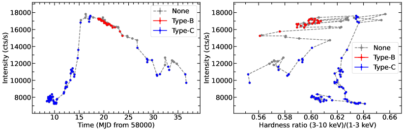
Figure 1: Light curve (left) and hardness-intensity diagram (right) of MAXI J1535$-$571 during the main outburst from MJD 58008 to 58037. Each point corresponds to a NICER orbit. The grey, red, and blue points indicate observations with, respectively, no QPO, type-B QPOs, and type-C QPOs. The error bars indicating 68% confidence level are smaller than the size of the points. The grey dashed lines connect the data points in time sequence.

Fig. 1 shows the light curve (left) and the HID (right) of MAXI J1535$-$571 in the time period MJD 58008–58036. Each data point corresponds to one NICER orbit. During the outburst, the source moves in an anticlockwise direction in the HID. From MJD 58008 to 58011, MAXI J1535$-$571 stays in the LHS with a count rate $\sim$ 8000 cts/s and a hardness ratio increasing from $\sim$ 0.6 to $\sim$ 0.64. From MJD 58011 to 58017 the count rate increases quickly from $\sim$ 7000 cts/s to $\sim$ 18000 cts/s while the hardness ratio increases slowly from $\sim$ 0.63 to $\sim$ 0.64 with some excursions up to a maximum of 0.66. At this point the source moves to the left in the HID and transits from the LHS to the HIMS (e.g. Belloni et al., 2005). From MJD 58017 to 58024 the count rate gradually decreases to $\sim$ 15000 cts/s, while the hardness ratio decreases from $\sim$ 0.62 to $\sim$ 0.56, indicating a state transition from the HIMS to a softer state. During the final part of the outburst, from MJD 58024 to 58036, the count rate continues decreasing gradually to 10000 cts/s, while the hardness ratio decreases from 0.6 to 0.56.

We mark with blue in Fig. 1 the observations where we detect the type-C QPOs. The data of the type-C QPOs are from Rawat et al. (2023) who performed a systematic study of the type-C QPOs in the NICER observations of MAXI J1535$-$571. The observations mark the hard and the hard-intermediate states, and do not include the observations of the soft-intermediate and the soft states where weak QPOs may appear (e.g. Belloni & Stella, 2014, for a review). In the top part of the HID (Fig. 1) we plot in grey observations with no significant QPO in the PDS. The remainder of the orbits, 26 in total, show a QPO with a rather constant frequency of $\sim$ 5–6 Hz. The information of the 26 orbits is listed in Tab. 3. We plot these observations in Fig. 1 with red. Since these QPOs in the SIMS are weak and their central frequencies are within a small range, to improve the signal-to-noise ratio we average the PDS of the 26 orbits. The left panel of Fig. 2 shows the averaged PDS. Based on the fact that both the QPO fundamental and the second harmonic appear and given the weak rms of the zero-centered broadband noise (0.7%; see Tab. 1), we tentatively identify these QPOs as type-B QPOs.

Since the red points in the HID (the right panel of Fig. 1) extend to a very soft region with hardness ratio less than 0.59, some of the QPOs we detected may be type-A (e.g. Casella et al., 2004). To check whether all our detections are type-B QPOs we divide the observations into two groups with hardness ratio either greater or smaller than 0.59. We find that in both groups the averaged PDS are consistent with the PDS shown in Fig. 2. We therefore conclude that all the QPOs that appear in the observations marked with red in Fig. 1 are type-B QPOs.

3.2 Initial fitting to the time-averaged energy spectra

We first fit all the energy spectra of the 26 orbits with the type-B QPOs separately using the model TBfeo*(diskbb+vKompthdk+gaussian), as introduced in subsection 2.2. The best-fitting values of $\Gamma$, $kT_{\text{in}}$ and the iron line profiles in the separate orbits are consistent with being the same within errors and only the normalizations of the Comptonized and the disk components change. Given that $kT_{\text{e}}$ cannot be constrained using the NICER spectra, we fix it to 250 keV.

Since the only parameters that change for the different orbits are the normalizations of the disk and the corona components, to improve the signal-to-noise ratio (SNR) we fit the energy spectra of the 26 orbits together, using the same model TBfeo*(diskbb+vKompthdk+gaussian) linking all the parameters in each of the 26 data groups, except for the normalizations of diskbb and vKompthdk components. Note that this fitting can also make it more convenient for our later joint fitting in subsection 3.4. This spectral fitting shows that, at this stage, the electron temperature of the corona $kT_{\text{e}}$ still cannot be constrained, therefore we fix it again to 250 keV. We find that the best-fitting hydrogen column density is $4.2\times 10^{22}$ $\text{cm}^{-2}$, consistent with previous measurements (Miller et al., 2018). The disk temperature is 1.14 keV, while the corona photon index is 2.84, indicating that the source is in a relatively soft state (Dong et al., 2022). The gaussian used to fit the iron line has a central energy of 6.8 keV with a width of 0.98 keV. For the 26 orbits, the 0.5–10 keV averaged flux of the disk and the Comptonized components is, respectively, $1.6\times 10^{-7}$ erg cm^-2 s^-1 and $0.4\times 10^{-7}$ erg cm^-2 s^-1.

3.3 Fractional rms and phase-lag spectra

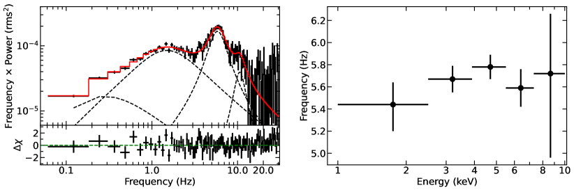
Figure 2: Left panel: Averaged PDS of MAXI J1535$-$571 in the 1–10 keV band for the NICER orbits listed in Tab. 3, with the best-fitting model and the residuals. The black points are the data and the red line is the best-fitting model. The dashed lines from the left to the right show two broadband noise, the type-B QPO fundamental and the second harmonic components. The residuals are the data minus the model divided by the error. Right panel: The QPO central frequency vs. energy for the type-B QPO. The error bars indicate the 68% confidence level.

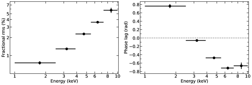
Figure 3: Fractional rms amplitude spectrum (left panel) and phase-lag spectrum (right panel) of the type-B QPO of MAXI J1535$-$571. The dashed grey line in the right panel marks the zero phase lag. In both panels, the vertical error bars indicates the 68% confidence level, while the horizontal error bars indicate the width of the energy channels.

As shown in the left panel of Fig. 2, we fit the PDS with four Lorentzians representing two broadband noise components, the QPO fundamental, and the second harmonic. Tab. 1 gives the best-fitting parameters of the Lorentzians. The average type-B QPO has a central frequency of $5.64\pm 0.07$ Hz with a FWHM of $2.9\pm 0.3$ Hz. The type-B QPO is weak, with an rms of $1.1\pm 0.05\%$. The second harmonic of the type-B QPO appears at a central frequency of $10.5\pm 0.5$ Hz, consistent with being twice the central frequency of the QPO fundamental.

We plot the rms spectrum of the QPO in the left panel of Fig. 3. The horizontal error bars are the width of the energy channels. As the energy increases from 1 keV to 10 keV, the rms increases monotonically from $\sim 1\%$ to $\sim 6\%$, indicating that the type-B QPO is mainly modulated by the hot corona.

The right panel of Fig. 3 shows the phase-lag spectrum of the type-B QPO. The horizontal error bars are the width of the energy channels. As the energy increases from 1 keV to 7.3 keV, the phase lags decrease from 0.8 rad to -0.7 rad, while above 7.3 keV the phase lags increase slightly to around -0.6 rad, resulting in a minimum in the phase-lag spectrum at around 6–7 keV. The energy where the minimum phase lag appears is consistent with the results of Stevens et al. (2018). The phase lag with respect to the the 1–10 keV reference band crosses the zero line (grey dashed line in the right panel of Fig. 3) from the positive to the negative at an energy of $\sim$ 3 keV.

Table 1: The parameters of the Lorentzians used to fit the averaged PDS of MAXI J1535$-$571. The error bar indicates the 1-$\sigma$ confidence level.

Component	Frequency (Hz)	FWHM (Hz)	rms (%)
QPO	$5.64\pm 0.07$	$2.9\pm 0.3$	$1.11\pm 0.05$
Harmonic	$10.5\pm 0.5$	$3\pm 2$	$0.43\pm 0.08$
BBN1∗	$0$	$0.5\pm 0.1$	$0.73\pm 0.08$
BBN2∗	$0.8\pm 0.1$	$2.5\pm 0.2$	$1.40\pm 0.07$

• BBN: Broadband noise component.

3.4 Joint fitting of the rms and phase-lag spectra of the QPO and the energy spectra of the source

Similar to what we did in Zhang et al. (2022), we fit jointly the rms and phase-lag spectra of the QPO and the energy spectra of the 26 orbits of MAXI J1535$-$571 (the latter are initially fitted in subsection 3.2) using the model TBfeo*(diskbb+vKompthdk+gaussian).

Note that for the fitting of the rms spectrum, vKompthdk is multiplied by a dilution component which is not explicitly written in the total model. The introduction of the dilution model is justified since the time-dependent Comptonization model computes the rms spectrum of a variable corona but the observed rms is reduced by all the non-variable spectral components. Here, we assume that the diskbb and the gaussian components are not variable, and therefore the dilution component is $\text{Flux}_{\text{Compt}}(E)/\text{Flux}_{\text{Total}}(E)$ such that $\text{rms}_{\text{Obs}}=\text{rms}_{\text{Compt}}*\text{Flux}_{\text{Compt}}/\text{Flux}_{\text{Total}}$. (Note that this dilution component does not introduce any new parameters to the fits.)

Initially, when we fit simultaneously the energy spectra of the 26 orbits and the rms and the phase-lag spectra of the QPO, $kT_{\text{s}}$ in vKompthdk is linked to $kT_{\text{in}}$ in diskbb. The fit yields a relatively large $\chi^{2}=104.0$ using 10 bins for the timing spectra and a corona size of $\sim 10^{4}$ km. The large corona size indicates that the softer seed photons from the outer part of the disk play an important role in producing the phase lags. Therefore, we let $kT_{\text{s}}$ in vKompthdk linked with $kT_{\text{in}}$ in diskbb to fit the energy spectra of the 26 orbits, but allow $kT_{\text{s}}$ to vary freely when fitting the rms and phase-lag spectra. We show a comparison of the best-fitting results of the cases with $kT_{\text{s}}=kT_{\text{in}}$ and $kT_{\text{s}}$ free in Fig. 4. Letting $kT_{\text{s}}$ free gives a significantly better fit, $\chi^{2}=62.3$ (Tab. 2), with $kT_{\text{s}}=0.59\pm 0.07$ keV, lower than $kT_{\text{in}}=1.139\pm 0.002$ keV; the corona is still relatively large with a size of $6500\pm 500$ km. In the time-averaged energy spectrum $kT_{\text{in}}$ and $\Gamma$ are the same as when $kT_{\text{s}}=kT_{\text{in}}$. The feedback fraction pegs at the upper boundary 1, which gives $\eta_{\text{int}}=0.33\pm 0.02$. (For an explanation of the difference between the $\eta$ and $\eta_{\text{int}}$, see section 1.) This means that $\sim 33\%$ of the corona photons return to the accretion disk where they are thermalized and re-emitted, resulting in a soft lag, while the other 67% of the corona photons are the observed Comptonized photons. The temperature of the inner disk, $kT_{\text{in}}=1.139\pm 0.002$ keV, and the photon index, $\Gamma=2.91\pm 0.06$, indicate that the source is in a relatively soft state. The spectral state matches well with the fact that the type-B QPO appears in the SIMS. Since we now include the rms and phase-lag spectra of the QPO and let $kT_{\text{s}}$ free in the fits, we try to let $kT_{\text{e}}$ free. From the joint fitting, we measure a hot corona with temperature $kT_{\text{e}}=330\pm 50$ keV, which is consistent with the corona temperature measured by Dong et al. (2022) in the SIMS of MAXI J1535$-$571 using the broadband data of NuSTAR and Insight-HXMT.

From the values of $kT_{\text{e}}$ and $\Gamma$ from Model 2, the optical depth of the corona is $\tau=0.16$ and the Compton y-parameter is $y=0.41$, indicating that the system is in the unsaturated Comptonization regime. This is consistent with the assumptions of the time-dependent Comptonization model vKompthdk that we used.

We note that, although a fit with a dual corona (see García et al., 2021) may reduce further the $\chi^{2}$, we do not explore it here because of the limited number of energy bands in the rms and phase-lag spectra of the QPO and the large number of free parameters that would be involved.

Since the corona is large, it should illuminate the outer part of the disk and produce a narrow iron line due to reflection off cold material there (e.g. Miller et al., 2018). Therefore, we add an extra Gaussian line to Model 1, which then becomes Model 2: TBfeo*(diskbb+vKompthdk+gaussian1+gaussian2). We find that a second Gaussian line centered at $6.62\pm 0.02$ keV with a width of $0.12\pm 0.02$ keV fits the data well. The significance of the narrow Gaussian line, measured as the ratio of the line normalization to its error, is 5 $\sigma$ and an F-test yields a probability of $1.8\times 10^{-9}$, which indicates that the narrow Gaussian line improves the fit significantly. The final results of the fitting are plotted in Fig. 5 and the parameters are given in Tab. 2.

To test a possible degeneracy of the parameters, we run an MCMC simulation for Model 2, using the Goodman-Weare chain algorithm (Goodman & Weare, 2010). After testing the convergence of the chain, we set the chain length to 240000 with 1200 walkers. We discard the first 120000 steps and record the last 120000 steps. The entire covariance matrix is divided by a factor of 10000 to ensure that the walkers initially sample a large range of the parameter space. Fig. 6 shows the results of the MCMC simulation. The inner disk temperature, $kT_{\text{in}}$, is somewhat covariant with the Galactic absorption, $N_{\text{H}}$, which is expected since the absorption influences mainly the soft part of the spectrum, while the outer disk temperature, $kT_{\text{s}}$, is covariant with the corona temperature, $kT_{\text{e}}$, since these two temperatures play an important role when computing the phase lags (Bellavita et al., 2022). For the corona geometry, the size of the corona may be modulated by the seed photons from the outer disk and the hot corona temperature. The feedback fraction reaches its upper limit and a 3-$\sigma$ error also constrain the feedback fraction to be larger than 0.9. Since the external heating rate maintains the temperature of the system when describing the timing spectra, $\delta\dot{H}_{\text{ext}}$ is correlated with the outer disk temperature, $kT_{\text{s}}$, the corona temperature, $kT_{\text{e}}$, and the corona size, $L$; the latter is always large, between 5600 km and 7200 km.

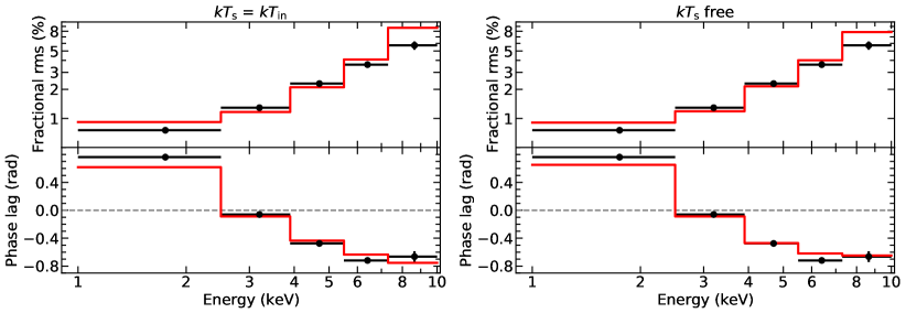
Figure 4: A comparison of the best-fitting model to the rms spectra (upper panels) and phase-lag spectra (lower panels) in the case in which $kT_{\text{s}}=kT_{\text{in}}=1.141$ keV (left panels) and $kT_{\text{s}}$ is free (right panels). In the case in which $kT_{\text{s}}=kT_{\text{in}}$, $\chi^{2}=104.0$ for 10 bins, while in the case in which $kT_{\text{s}}$ is free, $\chi^{2}=62.3$ for 10 bins. The data and the best-fitting model are in black and red, respectively.

Figure 5: The joint fitting of MAXI J1535$-$571 using NICER data. From top to bottom, the left panels show, respectively, the energy spectra of the 26 orbits, and the rms and phase-lag spectra of the type-B QPO with the best-fitting models. The right panels show the residuals with respect to the best-fitting model.

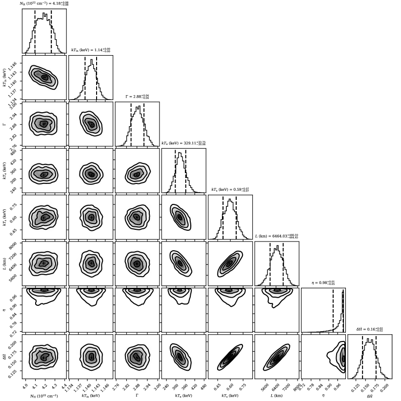
Figure 6: MCMC simulation of the spectral parameters of MAXI J1535$-$571. The contours in each panel indicate the 1-$\sigma$, 2-$\sigma$ and 3-$\sigma$ confidence ranges. The parameters are the same as those in the Model 2 in Tab. 2.

Table 2: Spectral parameters of the joint fitting for MAXI J1535$-$571. The error indicates the 1-$\sigma$ confidence level. See the text for more details about the parameters.

Component	Parameter	Model 1	Model 2
TBfeo	$N_{\text{H}}$ ($10^{22}$ cm-2)	$4.18\pm 0.08$	$4.18\pm 0.08$
	$A_{\text{O}}$	$0.44\pm 0.05$	$0.52\pm 0.05$
	$A_{\text{Fe}}$	$1.74\pm 0.08$	$1.51\pm 0.09$
diskbb	$kT_{\text{in}}$ (keV)	$1.138\pm 0.002$	$1.139\pm 0.002$
vKompthdk	$kT_{\text{s}}$ (keV)	$0.59\pm 0.06$	$0.59\pm 0.07$
	$kT_{\text{e}}$ (keV)	$330\pm 50$	$330\pm 30$
	$\Gamma$	$2.91\pm 0.06$	$2.88\pm 0.04$
	$L$ ($10^{3}$ km)	$6.5\pm 0.4$	$6.5\pm 0.5$
	$\eta^{\text{a}}$	$1_{-0.07}$	$1_{-0.07}$
	$\delta\dot{H}$	$0.15\pm 0.02$	$0.16\pm 0.02$
gaussian1	LineE (keV)	$6.80\pm 0.04$	$6.75\pm 0.05$
	$\sigma$ (keV)	$0.96\pm 0.04$	$1.01\pm 0.05$
	Norm ($10^{-2}$)	$6.2\pm 0.5$	$5.9\pm 0.4$
gaussian2	LineE (keV)		$6.62\pm 0.02$
	$\sigma$ (keV)		$0.14\pm 0.02$
	Norm ($10^{-3}$)		$3.0\pm 0.7$
$\chi^{2}/\text{bin}$ (SSS${}^{\text{b}}$)		4137.84 / 4576	4098.42 / 4576
$\chi^{2}/\text{bin}$ (rms${}^{\text{c}}$)		46.76 / 5	45.81 / 5
$\chi^{2}/\text{bin}$ (phase lag${}^{\text{d}}$)		15.57 / 5	15.47 / 5
$\chi^{2}/\text{d.o.f.}$		4200.08 / 4520	4159.70 / 4517
Disk flux${}^{\text{e}}$ (erg cm-2 s-1)		$1.577\pm 0.004\times 10^{-7}$
Corona flux${}^{\text{e}}$ (erg cm-2 s-1)		$0.444\pm 0.003\times 10^{-7}$

• We give only the negative error of the feedback fraction, $\eta$, because the parameter is consistent with 1, the maximum possible value at the 1-$\sigma$ confidence level.

• Steady-state spectrum.

• Fractional rms spectrum.

• Phase-lag spectrum.

• Unabsorbed flux.

4 Discussion

We have analyzed 36 NICER observations of the black hole candidate MAXI J1535$-$571 during the 2017/2018 outburst. We identify a type-B QPO in 26 NICER orbits where the source is in the SIMS, during which the inner disk is relatively hot, $kT_{\text{in}}\sim 1.1$ keV, and the corona photon index is relatively high, $\Gamma\sim 2.9$. From the simultaneous fit of the energy spectra of the source and the rms and phase-lag spectra of the type-B QPO, we find that the corona has a size $L=6500\pm 500$ km and a feedback fraction $\eta=1_{-0.07}$. We detect an additional significant narrow iron line with central energy of $\sim 6.6$ keV and FWHM of $\sim 0.1$ keV, consistent with a large corona illuminating the outer and cooler parts of the accretion disk.

4.1 The phase-lag spectrum of type-B QPOs

By systematically studying the type-B QPOs using RXTE data, the lags of type-B QPOs are hard for the BHB systems of low inclination angle, while they are either hard or soft for the BHB systems of high inclination angle (Van den Eijnden et al., 2017; Gao et al., 2017). The hard lags are likely due to inverse-Compton scattering of the soft disk photons in the corona (Kylafis et al., 2008), while the soft lags are likely due to the down-scattering of the hard photons in the disk (Uttley et al., 2014). Stevens & Uttley (2016) studied the hard lags of type-B QPOs in GX 339$-$4 using RXTE data and suggested that a corona with a large-scale height ($\sim 1.8\times 10^{4}$ km) is the jet base. This scenario of a large corona derived from the phase-resolved spectroscopy of the type-B QPO is later modeled by Kylafis et al. (2020) who proposed that the type-B QPO in GX 339$-$4 originates from a precessing jet. Note that RXTE is not sensitive to photons below 2–3 keV. Using NICER observations of MAXI J1348$-$630, Belloni et al. (2020) found that the phase lags are positive both in the 3–10 keV and the 0.7–2 keV with respect to the reference band at 2–3 keV. The positive phase lags in the 0.7–2 keV band exclude the possibility that the type-B QPOs are due to propagation of mass accretion rate fluctuations which, in this scenario, the phase lags below 2 keV relative to the 2–3 keV band should be negative. Comptonization of the soft photons in the corona naturally explains the positive lags at energy above 3 keV, while Belloni et al. (2020) suggested that the positive lags of the type-B QPO below 2 keV in MAXI J1348$-$630 could be due to Compton down-scattering in the corona by using Monte Carlo simulations assuming a flat seed spectrum between 2 and 3 keV. However, because their seed spectrum does not emit below 2 keV, they neglected the effect of the direct emission of the seed source on the phase-lag spectrum. Indeed, the direct emission of a more realistic seed source (e.g. an accretion disc) leads to a flat phase-lag spectrum below $\sim$ 3 keV (Kylafis, priv. comm.; see also Figure 1 in Bellavita et al., 2022), contrary to the observations.

From the phase-lag spectrum (right panel of Fig. 3) in MAXI J1535$-$571, the phase lags generally decrease as the energy increases, with the lags being a minimum at around 6 keV. If we take the lowest energy band (1–2.5 keV) as the reference band, in MAXI J1535$-$571 all the lags are soft. Stevens et al. (2018) proposed that the soft lags of the type-B QPOs in MAXI J1535$-$571 are due to the phase offset between the peaks in the corona emission and the modulation of the disk spectrum. Based on the fitting results of our vKompthdk model, we find that $33\%\pm 2\%$ of the corona photons return to and are reprocessed in the accretion disk, producing the soft lags. Therefore, the observed soft lags can be explained as the light-crossing time of a large corona illuminating the disk. Note that the minimum in the phase-lag spectrum at $\sim$ 6 keV could be related to the iron line feature, but since the type-B QPO in this source is weak, we do not have good enough resolution to perform a detailed line analysis.

4.2 Comparison of corona models of variability

X-ray variability in the accreting X-ray binaries is generally classified as broadband noise and QPOs (Ingram & Motta, 2019, for a review). The broadband noise at low frequencies usually shows large hard lags that are thought to be due to Comptonization, while at relatively high frequencies it sometimes shows soft lags, which have been proposed to be caused by X-ray reverberation of corona photons reflected off the accretion disk (Uttley et al., 2014). In a lamppost geometry of the corona above a black hole, the model reltrans calculates the difference in the light-travel time of the photons reflected off the accretion disk relative to the corona photons that travel directly to the observer (Ingram et al., 2019). This model is able to fit the time-lag spectrum of the broadband noise in the black hole X-ray transient MAXI J1820+070, giving a corona height of up to $\sim$ 500 $R_{\text{g}}$ (Wang et al., 2021), equivalent to $\sim$ 6400 km for an 8.5-$M_{\odot}$ black hole (Torres et al., 2020). The lamppost geometry of the corona is a simplification to allow the calculation of the ray tracing in the spacetime around the black hole. On the other hand, this model cannot explain the hard lags observed sometimes in these systems that are therefore assigned to either Comptonization or fluctuation of accretion propagation (Arévalo & Uttley, 2006; Kylafis et al., 2008). Since the soft (reverberation) and the hard (inverse-Compton scattering and mass accretion rate fluctuation) are treated separately, the model is in essence two separate mechanisms that are connected by the fitting procedure.

From the perspective of QPOs that dynamically originate from the L-T precession, Ingram et al. (2016) and Nathan et al. (2022) developed a tomographic model that fits the QPO phase-dependent energy spectrum, explaining the energy shifts of the observed iron $K_{\alpha}$ emission line in different QPO phases. Using NICER and NuSTAR data of GRS 1915+105 with a QPO frequency at 2.2 Hz, Nathan et al. (2022) measured a thermalization time delay of 70 ms, which is too long since in this long time delay the QPO signal would be washed out. Nathan et al. (2022) attributed this problem to the oversimplification of the precessing corona model. For instance, the authors did not take into account the precessing corona/jet obscuring different disk azimuths, which would result in a variation of the shape of the observed disk spectrum, and they ignored the light-crossing delays which can be of the order of milliseconds. Systematic error in the spectral modeling would potentially affect the measured time lags as well. Nathan et al. (2022) also measured an inner radius, $R_{\text{in}}=1.5R_{\text{g}}$, of the accretion disk which is too small to produce the 2.2-Hz QPO predicted by the L-T precession of the corona lying inside a truncated disk (Ingram et al., 2009). It could be that the corona is not horizontally, but more likely vertically, extended in the form of a jet-like structure, namely the outflow (Stevens & Uttley, 2016; Kylafis et al., 2020).

Regardless of the dynamical origin of the QPOs, the time-dependent Comptonization model vKompthdk developed by Karpouzas et al. (2020) and Bellavita et al. (2022) describes both the hard and soft lags by considering inverse-Compton scattering in the corona and thermal reprocessing in the disk. Since the model solves the linearized Kompaneets equation, it provides the distribution of photons in energy at any given time, regardless of the history of these photons via a single mechanism. This model can successfully fit the steady-state Comptonization spectrum and the rms and phase-lag spectra of QPOs with energies in the 1–100 keV range (Karpouzas et al., 2020; García et al., 2021; Méndez et al., 2022; García et al., 2022a; Zhang et al., 2022). A limitation of the model is that even though it considers the thermal reprocessing of hard photons in the accretion disk, it ignores the relativistic reflection that produces the atom florescent emission lines and Compton hump (García et al., 2014). The corona size measured by vKompthdk is generally big compared with the corona size predicted by L-T precession inside the truncated disk (see supplementary Fig. 4 in Méndez et al. 2022 and Fig. 5 in García et al. 2022a). If the corona size is large, regardless of the feedback fraction, a big corona is likely to be vertically extended (Méndez et al., 2022; Zhang et al., 2022). A dual-Comptonization model is also used to fit the NICER data of the type-B QPO of MAXI J1348$-$630 (García et al., 2021), showing that the inner part of the corona is small ($L\simeq 400$ km) and spherical or slab, with the hard photons efficiently returning to the accretion disk, while the outer part of the corona is large ($L\simeq 10^{4}$ km) and jet-like with nearly no hard photon feedbacking onto the accretion disk. The corona geometry, e.g. the size, measured from different models mentioned above has features in common (see below).

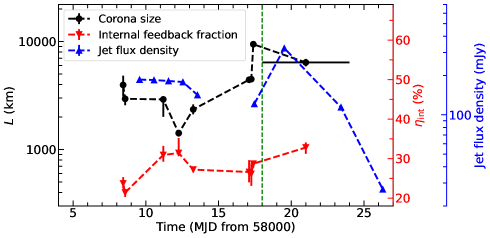
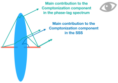
Figure 7: Left panel: The evolution of the corona geometry and the jet flux from the HIMS to the SIMS in MAXI J1535$-$571. The black, red, and blue points indicate the corona size, the intrinsic feedback fraction, and the jet flux density, respectively. The blue dashed line is discontinuous since the jet is quenched from MJD 58009 to 58017. The green dashed line indicates the time of the transition from the HIMS to the SIMS. Right panel: A schematic figure of the corona geometry of MAXI J1535$-$571 in the SIMS. The inner part of the disk provides the seed photons to the Comptonized emission that dominates the steady-state energy spectrum of the source, while the outer parts of the disk provide the seed photons to the Comptonized emission that dominates the rms and phase-lag spectra of the QPO. See text for more details.

4.3 Corona geometry

Fast transitions between type-B and other types (A and C) QPOs are often observed (e.g. Casella et al., 2004; Zhang et al., 2021). The detailed spectral-timing analysis of H 1743$-$322 indicates that the transition from type-B to type-C QPOs could be explained by the presence of a jet or a vertically extended optically thick Comptonization region (Harikrishna & Sriram, 2022). From a spectral-timing analysis of the Insight-HXMT data of MAXI J1348$-$630 in the SIMS, Liu et al. (2022) proposed a vertically extended corona that is the base of the jet, and explained the disappearance and appearance of the type-B QPO as the jet being parallel to the BH spin axis or not, due to the Bardeen-Petterson effect. In our study of MAXI J1535$-$571 in the SIMS, we notice that the type-B QPOs disappear in some NICER orbits as shown in Fig. 1 which may be explained by the L-T precession of the corona or the jet proposed by Liu et al. (2022).

The modeling of the corona through type-B QPOs in MAXI J1348$-$630 shows that the size of the jet-like corona is $\sim 10^{4}$ km (García et al., 2021). This size is comparable with the corona size of $6500\pm 500$ km that we find in MAXI J1535$-$571. The intrinsic feedback fraction in this work is $33\%\pm 2\%$, which indicates that the corona should be covering the accretion disk to some extent, as shown in the right panel of Fig. 7. From the fitting results in Tab. 2, the inner disk provides the seed photons and the Comptonized photons contribute mainly to the steady-state energy spectrum, while the outer disk provides relatively cold seed photons and the long light-crossing time of the Comptonized photons contribute mainly to the phase-lag spectrum. In MAXI J1535$-$571 we have already measured the corona geometry through type-C QPOs in the HIMS from MJD 58008 to 58017 (Zhang et al., 2022). The left panel of Fig. 7 shows the corona size, intrinsic feedback fraction, and the 9-GHz jet flux density (Russell et al., 2019) using the results both in Zhang et al. (2022) and this work. Note that we have converted the feedback fraction, $\eta$, into the intrinsic feedback fraction, $\eta_{\text{int}}$. As discussed in  Zhang et al. (2022), the corona on MJD 58017 is a vertically extended, jet-like corona, which expands vertically to its maximal size, $L\sim 9300$ km, with $\eta_{\text{int}}\sim 28\%$, two days before the transient jet reaches the maximum flux density. After MJD 58017, MAXI J1535$-$571 transits into the SIMS. In the SIMS from MJD 58018 to 58024, we measure a corona size $L\sim 6500$ km with $\eta_{\text{int}}\sim 33\%$. Compared to the corona geometry in the end of the HIMS on MJD 58017, in the SIMS the corona size contracts and the hard photons feedback onto the disk more efficiently, indicating that the corona contracts vertically and expands horizontally. After MJD 58024 no QPO appears in the intermediate and high-soft states and the transient jet flux density gradually decays until it is no longer detected. The change of the morphology of the corona geometry in the SIMS, together with that in the HIMS, and the change of the jet flux density, suggests that the increasing size of the jet-like corona may give rise to the large-scale transient jet ejecta lagging behind the change of the corona size. After the ejection, the corona in the jet base contracts and the transient jet loses its energy source so the observed radio flux density drops. This suggests a connection between the corona and the jet.

The corona-jet connection has been investigated using vKompthdk through type-C QPOs in GRS 1915+105 with 12-year RXTE observations (Karpouzas et al., 2021; Méndez et al., 2022; García et al., 2022a). The connection between the corona and the jet in the persistent source GRS 1915+105 is similar to that in the BH X-ray transient MAXI J1535$-$571. In GRS 1915+105, when the radio emission is weak the corona covers large parts of the accretion disk and the hard photons efficiently feedback onto the disk, while when the radio emission is strong the corona is vertically extended and jet-like, and less hard photons feedback onto the disk (Méndez et al., 2022). The only difference is that, in the SIMS of MAXI J1535$-$571, the hard photons feedback onto the disk more efficiently than in the HIMS. The $\sim 33\%$ intrinsic feedback fraction in the SIMS of MAXI J1535$-$571 is similar to the $\sim 35\%$ intrinsic feedback fraction in the SIMS of MAXI J1348$-$630 (García et al., 2021; Bellavita et al., 2022). In fact the feedback fraction of hard photons may either decrease or increase, depending on the balance between the Compton cooling process in the disk and the heating up of the corona (Merloni & Fabian, 2001; Karpouzas et al., 2020).

The evolution of the corona height using the light-crossing delays in reverberation shows quite a similar trend to our measurements using vKompthdk through the QPOs. Wang et al. (2022) studied archival data of 10 black hole candidates with NICER and found that during the hard to intermediate state transition the soft lags first decrease and then increase (see Fig. 6 in Wang et al., 2022). Assuming a lamppost geometry, the corona height in the hard state decreases from $\sim 1000$ km to $\sim 200$ km, in the HIMS it increases monotonically up to 9000 km, and in the SIMS it decreases slightly to $\sim 6000$ km. Comparing these results with those in the left panel of Fig. 7, we notice a general consistence of the measurements of the corona size. This consistence suggests the possibility to combine reltrans and vKompthdk to measure the corona geometry when reverberation lags and QPOs appear simultaneously.

Data Availability

The X-ray data used in this article are accessible at NASA’s High Energy Astrophysics Science Archive Research Center https://heasarc.gsfc.nasa.gov/. The software GHATS for Fourier timing analysis is available at http://www.brera.inaf.it/utenti/belloni/GHATS_Package/Home.html. The time-dependent Comptonization model and the generator of the MCMC corner plot are available at the GitHub repositories https://github.com/candebellavita/vkompth and https://github.com/garciafederico/pyXspecCorner.

Appendix A Observations and orbits used for concatenation

Table 3: NICER observations and QPO frequency of MAXI J1535$-$571. The error bars indicate the 1-$\sigma$ confidence level.

Observation ID	Orbit	MJD start	QPO frequency (Hz)
1050360114	1	58018.88	$6.1\pm 0.1$
	2	58018.94	$6.7\pm 0.4$
1050360115	1	58019.01	$6.2\pm 0.4$
	4	58019.22	$5.6\pm 0.4$
	5	58019.28	$5.5\pm 0.5$
	6	58019.47	$5.7\pm 0.3$
	7	58019.54	$5.5\pm 0.3$
	8	58019.60	$5.3^{+0.6}_{-0.1}$
	13	58019.92	$5.2\pm 0.5$
	14	58019.99	$6.0\pm 0.2$
1050360116	1	58020.05	$5.6\pm 0.5$
	4	58020.25	$5.1\pm 0.2$
	5	58020.31	$5.5\pm 0.4$
	6	58020.37	$5.8\pm 0.2$
	8	58020.50	$6.2\pm 0.2$
1050360117	2	58021.15	$6.2\pm 0.4$
	3	58021.40	$5.3\pm 0.2$
	4	58021.60	$5.8\pm 0.3$
	5	58021.77	$5.5^{+0.1}_{-0.5}$
1050360118	1	58022.24	$6.0\pm 0.2$
1050360119	1	58023.26	$6.1\pm 0.1$
	3	58023.77	$5.1\pm 0.1$
1050360120	1	58020.57	$6.6\pm 0.4$
	2	58020.63	$5.8\pm 0.2$
	4	58020.76	$5.6\pm 0.2$
	7	58020.95	$4.8\pm 0.1$

References

- Alabarta et al. (2021) Alabarta K., et al., 2021, MNRAS, 507, 5507
- Alabarta et al. (2022) Alabarta K., Méndez M., García F., Peirano V., Altamirano D., Zhang L., Karpouzas K., 2022, MNRAS, 514, 2839
- Arévalo & Uttley (2006) Arévalo P., Uttley P., 2006, MNRAS, 367, 801
- Arnaud (1996) Arnaud K. A., 1996, in Jacoby G. H., Barnes J., eds, Astronomical Society of the Pacific Conference Series Vol. 101, Astronomical Data Analysis Software and Systems V. p. 17
- Bambi et al. (2021) Bambi C., et al., 2021, Space Sci. Rev., 217, 65
- Bellavita et al. (2022) Bellavita C., García F., Méndez M., Karpouzas K., 2022, MNRAS, 515, 2099
- Belloni (2010) Belloni T. M., 2010, in Belloni T., ed., , Vol. 794, Lecture Notes in Physics, Berlin Springer Verlag. p. 53, doi:10.1007/978-3-540-76937-8_3
- Belloni & Hasinger (1990) Belloni T., Hasinger G., 1990, A&A, 230, 103
- Belloni & Motta (2016) Belloni T. M., Motta S. E., 2016, in Bambi C., ed., Astrophysics and Space Science Library Vol. 440, Astrophysics of Black Holes: From Fundamental Aspects to Latest Developments. p. 61 (arXiv:1603.07872), doi:10.1007/978-3-662-52859-4_2
- Belloni & Stella (2014) Belloni T. M., Stella L., 2014, Space Sci. Rev., 183, 43
- Belloni et al. (2002) Belloni T., Psaltis D., van der Klis M., 2002, ApJ, 572, 392
- Belloni et al. (2005) Belloni T., Homan J., Casella P., van der Klis M., Nespoli E., Lewin W. H. G., Miller J. M., Méndez M., 2005, A&A, 440, 207
- Belloni et al. (2011) Belloni T. M., Motta S. E., Muñoz-Darias T., 2011, Bulletin of the Astronomical Society of India, 39, 409
- Belloni et al. (2020) Belloni T. M., Zhang L., Kylafis N. D., Reig P., Altamirano D., 2020, MNRAS, 496, 4366
- Bhargava et al. (2019) Bhargava Y., Belloni T., Bhattacharya D., Misra R., 2019, MNRAS, 488, 720
- Cao et al. (2022) Cao Z., Lucchini M., Markoff S., Connors R. M. T., Grinberg V., 2022, MNRAS, 509, 2517
- Casella et al. (2004) Casella P., Belloni T., Homan J., Stella L., 2004, A&A, 426, 587
- Casella et al. (2005) Casella P., Belloni T., Stella L., 2005, ApJ, 629, 403
- Chauhan et al. (2019) Chauhan J., et al., 2019, MNRAS, 488, L129
- Connors et al. (2019) Connors R. M. T., et al., 2019, MNRAS, 485, 3696
- Connors et al. (2020) Connors R. M. T., et al., 2020, ApJ, 892, 47
- Corbel et al. (2004) Corbel S., Fender R. P., Tomsick J. A., Tzioumis A. K., Tingay S., 2004, ApJ, 617, 1272
- Cúneo et al. (2020) Cúneo V. A., et al., 2020, MNRAS, 496, 1001
- Dauser et al. (2022) Dauser T., García J. A., Joyce A., Licklederer S., Connors R. M. T., Ingram A., Reynolds C. S., Wilms J., 2022, MNRAS, 514, 3965
- Done et al. (2007) Done C., Gierliński M., Kubota A., 2007, A&ARv, 15, 1
- Dong et al. (2022) Dong Y., Liu Z., Tuo Y., Steiner J. F., Ge M., García J. A., Cao X., 2022, MNRAS, 514, 1422
- Esin et al. (1997) Esin A. A., McClintock J. E., Narayan R., 1997, ApJ, 489, 865
- Fabian et al. (1989) Fabian A. C., Rees M. J., Stella L., White N. E., 1989, MNRAS, 238, 729
- Fender (2006) Fender R., 2006, in , Vol. 39, Compact stellar X-ray sources. pp 381–419
- Fender et al. (2004) Fender R. P., Belloni T. M., Gallo E., 2004, MNRAS, 355, 1105
- Fender et al. (2009) Fender R. P., Homan J., Belloni T. M., 2009, MNRAS, 396, 1370
- Ferreira (1997) Ferreira J., 1997, A&A, 319, 340
- Galeev et al. (1979) Galeev A. A., Rosner R., Vaiana G. S., 1979, ApJ, 229, 318
- Gallo et al. (2003) Gallo E., Fender R. P., Pooley G. G., 2003, MNRAS, 344, 60
- Gallo et al. (2012) Gallo E., Miller B. P., Fender R., 2012, MNRAS, 423, 590
- Gao et al. (2017) Gao H. Q., et al., 2017, MNRAS, 466, 564
- García et al. (2014) García J., et al., 2014, ApJ, 782, 76
- García et al. (2021) García F., Méndez M., Karpouzas K., Belloni T., Zhang L., Altamirano D., 2021, MNRAS, 501, 3173
- García et al. (2022a) García F., Karpouzas K., Méndez M., Zhang L., Zhang Y., Belloni T., Altamirano D., 2022a, MNRAS, 513, 4196
- García et al. (2022b) García J. A., Dauser T., Ludlam R., Parker M., Fabian A., Harrison F. A., Wilms J., 2022b, ApJ, 926, 13
- Gendreau et al. (2016) Gendreau K. C., et al., 2016, in den Herder J.-W. A., Takahashi T., Bautz M., eds, Society of Photo-Optical Instrumentation Engineers (SPIE) Conference Series Vol. 9905, Space Telescopes and Instrumentation 2016: Ultraviolet to Gamma Ray. p. 99051H, doi:10.1117/12.2231304
- Gilfanov (2010) Gilfanov M., 2010, in Belloni T., ed., , Vol. 794, Lecture Notes in Physics, Berlin Springer Verlag. p. 17, doi:10.1007/978-3-540-76937-8_2
- Goodman & Weare (2010) Goodman J., Weare J., 2010, Communications in Applied Mathematics and Computational Science, 5, 65
- Haardt & Maraschi (1991) Haardt F., Maraschi L., 1991, ApJ, 380, L51
- Harikrishna & Sriram (2022) Harikrishna S., Sriram K., 2022, MNRAS,
- Homan & Belloni (2005) Homan J., Belloni T., 2005, Ap&SS, 300, 107
- Homan et al. (2020) Homan J., et al., 2020, ApJ, 891, L29
- Huang et al. (2018) Huang Y., et al., 2018, ApJ, 866, 122
- Ingram (2019) Ingram A., 2019, MNRAS, 489, 3927
- Ingram & Motta (2019) Ingram A. R., Motta S. E., 2019, New Astron. Rev., 85, 101524
- Ingram & van der Klis (2013) Ingram A., van der Klis M., 2013, MNRAS, 434, 1476
- Ingram et al. (2009) Ingram A., Done C., Fragile P. C., 2009, MNRAS, 397, L101
- Ingram et al. (2016) Ingram A., van der Klis M., Middleton M., Done C., Altamirano D., Heil L., Uttley P., Axelsson M., 2016, MNRAS, 461, 1967
- Ingram et al. (2019) Ingram A., Mastroserio G., Dauser T., Hovenkamp P., van der Klis M., García J. A., 2019, MNRAS, 488, 324
- Kalemci et al. (2022) Kalemci E., Kara E., Tomsick J. A., 2022, arXiv e-prints, p. arXiv:2206.14410
- Kara et al. (2019) Kara E., et al., 2019, Nature, 565, 198
- Karpouzas et al. (2020) Karpouzas K., Méndez M., Ribeiro E. M., Altamirano D., Blaes O., García F., 2020, MNRAS, 492, 1399
- Karpouzas et al. (2021) Karpouzas K., Méndez M., García F., Zhang L., Altamirano D., Belloni T., Zhang Y., 2021, MNRAS, 503, 5522
- Kawamura et al. (2022) Kawamura T., Axelsson M., Done C., Takahashi T., 2022, MNRAS, 511, 536
- Kennea et al. (2017) Kennea J. A., Evans P. A., Beardmore A. P., Krimm H. A., Romano P., Yamaoka K., Serino M., Negoro H., 2017, The Astronomer’s Telegram, 10700, 1
- Kylafis & Reig (2018) Kylafis N. D., Reig P., 2018, A&A, 614, L5
- Kylafis et al. (2008) Kylafis N. D., Papadakis I. E., Reig P., Giannios D., Pooley G. G., 2008, A&A, 489, 481
- Kylafis et al. (2020) Kylafis N. D., Reig P., Papadakis I., 2020, A&A, 640, L16
- Leahy et al. (1983) Leahy D. A., Darbro W., Elsner R. F., Weisskopf M. C., Sutherland P. G., Kahn S., Grindlay J. E., 1983, ApJ, 266, 160
- Lee & Miller (1998) Lee H. C., Miller G. S., 1998, MNRAS, 299, 479
- Liu et al. (2022) Liu H. X., et al., 2022, ApJ, 938, 108
- Ma et al. (2021) Ma X., et al., 2021, Nature Astronomy, 5, 94
- Marcel et al. (2018) Marcel G., et al., 2018, A&A, 615, A57
- Marcel et al. (2019) Marcel G., et al., 2019, A&A, 626, A115
- Marcel et al. (2020) Marcel G., et al., 2020, A&A, 640, A18
- Markoff et al. (2001) Markoff S., Falcke H., Fender R., 2001, A&A, 372, L25
- Markoff et al. (2005) Markoff S., Nowak M. A., Wilms J., 2005, ApJ, 635, 1203
- Martocchia & Matt (1996) Martocchia A., Matt G., 1996, MNRAS, 282, L53
- Méndez & van der Klis (1997) Méndez M., van der Klis M., 1997, ApJ, 479, 926
- Méndez et al. (2022) Méndez M., Karpouzas K., García F., Zhang L., Zhang Y., Belloni T. M., Altamirano D., 2022, Nature Astronomy, 6, 577
- Merloni & Fabian (2001) Merloni A., Fabian A. C., 2001, MNRAS, 321, 549
- Meyer-Hofmeister et al. (2012) Meyer-Hofmeister E., Liu B. F., Meyer F., 2012, A&A, 544, A87
- Miller et al. (2018) Miller J. M., et al., 2018, ApJ, 860, L28
- Mirabel & Rodríguez (1994) Mirabel I. F., Rodríguez L. F., 1994, Nature, 371, 46
- Mitsuda et al. (1984) Mitsuda K., et al., 1984, PASJ, 36, 741
- Miyamoto et al. (1988) Miyamoto S., Kitamoto S., Mitsuda K., Dotani T., 1988, Nature, 336, 450
- Motta et al. (2012) Motta S., Homan J., Muñoz Darias T., Casella P., Belloni T. M., Hiemstra B., Méndez M., 2012, MNRAS, 427, 595
- Nakahira et al. (2017) Nakahira S., et al., 2017, The Astronomer’s Telegram, 10729, 1
- Nathan et al. (2022) Nathan E., et al., 2022, MNRAS, 511, 255
- Negoro et al. (2017) Negoro H., et al., 2017, The Astronomer’s Telegram, 10699, 1
- Nowak (2000) Nowak M. A., 2000, MNRAS, 318, 361
- Nowak et al. (1999) Nowak M. A., Vaughan B. A., Wilms J., Dove J. B., Begelman M. C., 1999, ApJ, 510, 874
- Peirano & Méndez (2022) Peirano V., Méndez M., 2022, MNRAS, 513, 2804
- Petrucci et al. (2008) Petrucci P.-O., Ferreira J., Henri G., Pelletier G., 2008, MNRAS, 385, L88
- Rawat et al. (2023) Rawat D., et al., 2023, arXiv e-prints, p. arXiv:2301.04418
- Reis et al. (2008) Reis R. C., Fabian A. C., Ross R. R., Miniutti G., Miller J. M., Reynolds C., 2008, MNRAS, 387, 1489
- Remillard et al. (2002) Remillard R. A., Sobczak G. J., Muno M. P., McClintock J. E., 2002, ApJ, 564, 962
- Remillard et al. (2022) Remillard R. A., et al., 2022, AJ, 163, 130
- Russell et al. (2019) Russell T. D., et al., 2019, ApJ, 883, 198
- Russell et al. (2020) Russell T. D., et al., 2020, MNRAS, 498, 5772
- Shapiro et al. (1976) Shapiro S. L., Lightman A. P., Eardley D. M., 1976, ApJ, 204, 187
- Sharma et al. (2018) Sharma R., Jaleel A., Jain C., Pandey J. C., Paul B., Dutta A., 2018, MNRAS, 481, 5560
- Stella & Vietri (1998) Stella L., Vietri M., 1998, ApJ, 492, L59
- Stevens & Uttley (2016) Stevens A. L., Uttley P., 2016, MNRAS, 460, 2796
- Stevens et al. (2018) Stevens A. L., et al., 2018, ApJ, 865, L15
- Sunyaev & Titarchuk (1980) Sunyaev R. A., Titarchuk L. G., 1980, A&A, 86, 121
- Tagger & Pellat (1999) Tagger M., Pellat R., 1999, A&A, 349, 1003
- Tao et al. (2018) Tao L., et al., 2018, MNRAS, 480, 4443
- Tetarenko et al. (2019) Tetarenko A. J., Casella P., Miller-Jones J. C. A., Sivakoff G. R., Tetarenko B. E., Maccarone T. J., Gandhi P., Eikenberry S., 2019, MNRAS, 484, 2987
- Tetarenko et al. (2021) Tetarenko A. J., et al., 2021, MNRAS, 504, 3862
- Torres et al. (2020) Torres M. A. P., Casares J., Jiménez-Ibarra F., Álvarez-Hernández A., Muñoz-Darias T., Armas Padilla M., Jonker P. G., Heida M., 2020, ApJ, 893, L37
- Uttley et al. (2014) Uttley P., Cackett E. M., Fabian A. C., Kara E., Wilkins D. R., 2014, A&ARv, 22, 72
- Van den Eijnden et al. (2017) Van den Eijnden J., Ingram A., Uttley P., Motta S. E., Belloni T. M., Gardenier D. W., 2017, MNRAS, 464, 2643
- Van der Klis (1989) Van der Klis M., 1989, in Ögelman H., van den Heuvel E. P. J., eds, NATO Advanced Study Institute (ASI) Series C Vol. 262, Timing Neutron Stars. p. 27
- Vaughan & Nowak (1997) Vaughan B. A., Nowak M. A., 1997, ApJ, 474, L43
- Verner et al. (1996) Verner D. A., Ferland G. J., Korista K. T., Yakovlev D. G., 1996, ApJ, 465, 487
- Wang-Ji et al. (2018) Wang-Ji J., et al., 2018, ApJ, 855, 61
- Wang et al. (2021) Wang J., et al., 2021, ApJ, 910, L3
- Wang et al. (2022) Wang J., et al., 2022, ApJ, 930, 18
- Wilms et al. (2000) Wilms J., Allen A., McCray R., 2000, ApJ, 542, 914
- Xu et al. (2018) Xu Y., et al., 2018, ApJ, 852, L34
- You et al. (2018) You B., Bursa M., Życki P. T., 2018, ApJ, 858, 82
- You et al. (2021) You B., et al., 2021, Nature Communications, 12, 1025
- Zdziarski et al. (1996) Zdziarski A. A., Johnson W. N., Magdziarz P., 1996, MNRAS, 283, 193
- Zdziarski et al. (2021) Zdziarski A. A., Dziełak M. A., De Marco B., Szanecki M., Niedźwiecki A., 2021, ApJ, 909, L9
- Zel’dovich & Shakura (1969) Zel’dovich Y. B., Shakura N. I., 1969, Soviet Ast., 13, 175
- Zhang et al. (2021) Zhang L., et al., 2021, MNRAS, 505, 3823
- Zhang et al. (2022) Zhang Y., et al., 2022, MNRAS, 512, 2686
- Życki et al. (1999) Życki P. T., Done C., Smith D. A., 1999, MNRAS, 309, 561