SimCGNN: Simple Contrastive Graph Neural Network for Session-based Recommendation

Abstract

Session-based recommendation (SBR) problem, which focuses on next-item prediction for anonymous users, has received increasingly more attention from researchers. Existing graph-based SBR methods all lack the ability to differentiate between sessions with the same last item, and suffer from severe popularity bias. Inspired by nowadays emerging contrastive learning methods, this paper presents a Simple Contrastive Graph Neural Network for Session-based Recommendation (SimCGNN). In SimCGNN, we first obtain normalized session embeddings on constructed session graphs. We next construct positive and negative samples of the sessions by two forward propagation and a novel negative sample selection strategy, and then calculate the constructive loss. Finally, session embeddings are used to give prediction. Extensive experiments conducted on two real-word datasets show our SimCGNN achieves a significant improvement over state-of-the-art methods.

1 Introduction

With the progressive development of the contemporary internet and the explosion of information on the Internet, recommender systems have become an essential component. Sequential recommender systems consider the dynamic preference development and take both user-level information and item-level information into consideration. In certain scenarios, however, the user can be anonymous, which means that we only have access to item-level features and user-level features are not visible. Session-based recommender, which observes only the current session rather than sufficient historical user-item interaction records, has drawn attention in recent years.

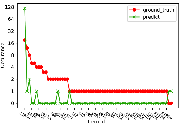
Figure 1: We trained SR-GNN on the diginetica dataset and selected a set of sessions (127 in total) with the same last-interacted item (item 33889, the most commonly occurred last-item) from the diginetica dataset for prediction. This line graph counts the number of occurrences of different items on the ground truth and model predicted values.

To capture the sequential relationship, Markov Chain (MC)-based sequential recommendersHe and McAuley (2016)Rendle et al. (2010) are the first to be proposed. However, due to limited representation ability and the strong reliance upon the last interacted item in each session, their performances are limited. Recurrent neural networks (RNNs) are then introduced into session-based recommendation thanks to their natural ability for modeling sequential information. With the introduction of GRU4RecHidasi et al. (2016), RNN turned out to be the structure of choice for solving the session recommendation problem, for example, NARMLi et al. (2017) designs two RNNs to capture user’s global and local sequential preference correspondingly. It was not until the existence of SR-GNNWu et al. (2019), which utilized a gated graph neural network (GGNN) to extract sequential information on a session graph. Since then, works following the basic schema of SR-GNN have been proposed. TAGNNYu et al. (2020) added a target-attentive mechanism onto SR-GNN and gain promising performance. Also, as SR-GNN focuses only on a local session, methods like FGNNQiu et al. (2019) and GCE-GNNWang et al. (2020) both utilize global information in session-based recommendation but in different ways.

Although all methods mentioned above have favorable results, they maintain a drawback inherited from the MC-based approach to the present day. That is the strong dependency upon the last interacted item. Take the classical SR-GNN as an example, when assembling the final session, it simply takes linear transformation over the concatenation of the embedding vector of the last-item and the global embedding vector. And as a result, these methods may have trouble in distinguishing between sessions that have the same last interacted item. As shown in Fig.1, we first trained an SR-GNN on the Diginetica dataset and then visualized the distribution of predicted labels and ground-truth labels of sessions that shares the same last-interacted item. This indicates a phenomenon that methods with this assembling techniques tends to predict the same items for sessions with the same last-item, despite of the underlying diversity. As we have mentioned earlier, a large branch of existing graph-based methods (Yu et al. (2020); Wang et al. (2020) for example) refers to the same approach as SR-GNN in the final assembly of the session embedding, resulting in this phenomenon will also be widespread in the current advanced graph-based SBR method. In this paper, we refer to this phenomenon as the ”same last-item confusion” problem. Apart from this, Fig.1 also proved the hypothesis proposed by Gupta et al. (2019) that the prediction of SR-GNN is likely to be affected by popularity bias.

To cope with the last-item, intuitively we tend to increase the discrepancy between sessions with the same last-item, which naturally fits the schema of constractive learning methods by considering sessions with the same last-item as negative samples. However, as positive samples are hard to define, we simply follows the idea of Gao et al. (2021) by treating the session itself as a positive sample through dropoutSrivastava et al. (2014) techniques. To this end, we proposed a novel session-based recommender namely Simple Contrastive Graph Neural Network for Session-based Recommendation (SimCGNN). Firstly, in order deal with the ”same last-item confusion” problem, we designed a novel contrastive module to increase the discrepancy between sessions with the same last interacted item. Secondly, to eliminate the advantage of popular items in the final prediction and to predict the underlying interest of the users themselves as much as possible, we normalised both the embedding of items and sessions.

Our main contributions in this paper are listed as follows.

1) We introduce a contrast learning approach to solve the last-item interaction confusion problem and propose a novel negative sample selection strategy.

2) To alleviate the popularity bias, we proposed normalized item embeddings and session embeddings.

3) Extensive experiments conducted on real-world datasets show that SimCGNN outperforms the sota methods and additional experiments also demonstrate the effectiveness of our approach for both of these two problems.

2 Related Work

2.1 Traditional Methods

A series of approaches Sarwar et al. (2001a); Salakhutdinov and Mnih (2007); Koren et al. (2009) based on matrix factorization (MF) are representatives of the traditional methods. MF-based methods consider that the user-item interaction matrix is too sparse and then decompose the matrix into two low-rank dense matrices, which correspond to users and items respectively. However, MF-based approaches do not model users’ sequential interaction behavior, and therefore not suitable for making sequential recommendations.

Given that static matrix decomposition methods do not model sequence behavior, FPMCRendle et al. (2010) models user behavior as a Markov Chain and combines Markov Chains with MF. FOSSILHe and McAuley (2016) improves on FPMC by introducing factorized sequential prediction with an item similarity model and higher-order Markov Chains, thus both long-term and short-term user behaviour are taken into account. However, due to expressive capability limitation of their shallow network, they do not perform well in nowadays more complex recommendation scenarios.

2.2 Deep Learning-Based Methods

In recent years, as deep-learning methods emerge, deep learning-based recommendation methodsSun et al. (2019); de Souza Pereira Moreira et al. (2021) utilizing recurrent neural networks (RNNs) are on the rise. GRU4RecHidasi et al. (2016) is a typical pioneer in utilizing RNN structure for making sequential recommendations. After that, more attempts have been made to perform sequential recommendations on RNNs. Tan et al.Tan et al. (2016) improved the performance of RNN recommendation models by proposing several data enhancements and training tricks. Li et al.Li et al. (2017) proposed a neural attentive recommendation machine with an encoder-decoder structure based on RNN to capture the user’s sequential preference. STAMPLiu et al. (2018), which deposits the RNN structure by using simple MLPs and attention mechanisms, proved to be efficient in capturing both users’ static and dynamic interests. Although deep learning-based models have more powerful representation capabilities than traditional methods, these approaches caanot still model complex item relationships, for example, non-adjacent item transitions.

2.3 Neural Network on Graphs

Recently, thanks to the rise of graph neural networksVelickovic et al. (2017); Chang et al. (2015); Dong et al. (2020), many approachesXu et al. (2019); Chen et al. (2022); He et al. (2020) use GNN-based network structures to solve SBR problems. SR-GNNWu et al. (2019) is one of the earliest and most representative ones, which models each session as a session graph, and applies a gated-GNNLi et al. (2016) to finally get a representative embedding of the session. After the great success of SR-GNN, many variants of SR-GNN have been proposed. For example, TAGNNYu et al. (2020) proposed a target-aware attention mechanism upon SR-GNN, which adaptively activates different user interests concerning varied target items. FGNNQiu et al. (2019) takes both sequence order and the latent order in the session graph into consideration. Disen-GNNLi et al. (2022) constructs a disentangled session graph to discover underlying session purpose. $S^{2}$-DHCNXia et al. (2021) leverages hypergraph techniques to represent each session and utilizes constractive learning techniques to perform self-supervised learning. Instead of utilizing local session graphs only, methods such as GCE-GNNWang et al. (2020) construct global graphs to obtain global information on the dataset. However, as mentioned in the previous section, all of these methods have serious ”same last-item confusion” problem and thus suffer from performance degradation.

3 Methodology

3.1 Problem Formulation

A session-based recommender is supposed to give recommendations to users based on the inputs of their anonymous historical interaction sequences, e.g. clicks or purchases. Given $\mathcal{V}=\left\{v_{1},v_{2},...,v_{m}\right\}$ as the item set, an anonymous interaction session $s$ is an item sequence $s_{i}=[v_{1}^{i},v_{2}^{i},...,v_{|s_{i}|}^{i}],s_{i}\in\mathcal{S}$, where $v_{j}^{i}$ is the $j$-th interacted item of the $i$-th session. Given session $s_{i}$, our goal is to predict $v_{|s_{i}|+1}^{i}$.

3.2 Overview

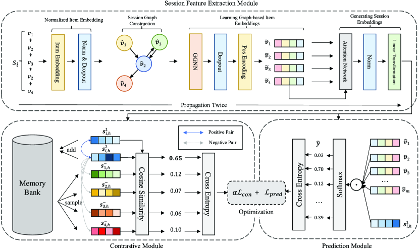
Figure 2: The overall network architecture of SimCGNN.

The overall workflow of our proposed SimCGNN is illustrated in Fig.2.

3.3 Session Feature Extraction Module

3.3.1 Normalized Item Embedding

Since the one-hot vectors of items are sparse and high-dimensional and do not carry pairwise distance information, we first embed each item $v_{i}\in\mathcal{V}$ into a $d$-dimensional representation $\bm{v}_{i}\in\mathbb{R}^{d}$.

As some existing methods directly utilize $\bm{v}_{i}$ for downstream tasks, we argue that the direct use of embedded vectors would lead to popularity bias Gupta et al. (2019). To this end, we intuitively add $L_{2}$ normalization to the raw feature vector. Apart from this, we also add Dropout directly on embedding layer for the downstream contrastive module. The normalized vectors $\hat{\bm{v}}_{i}$ are given as follows:

$$\hat{\bm{v}}_{i}=Dropout(Norm(\bm{v}_{i}),p)$$ (1)

where $p$ is the dropout probability, $Norm(\cdot)$ is the L2-normalization function.

3.3.2 Session Graph Construction

To explore rich transitions among items and generate accurate latent vectors of items, we model each session $s$ as a directed graph $\mathcal{G}_{s}=(\mathcal{V}_{s},\mathcal{E}_{s})$, where each node $v_{s,i}\in\mathcal{V}_{s}$ represents an item and each edge $(v_{s,i-1},v_{s,i})\in\mathcal{E}_{s}$ represents a user interact $v_{s,i}$ after the interaction of $v_{s,i-1}$. To deal with items that occurs multiple times in sessions, we assign a normalized weight to each edge. The weight is calculated by the occurrence of the corresponding interaction ($(v_{s,i-1},v_{s,i})$) divides the out-degree of the starting node ($v_{s,i-1}$). We use the previously obtained embedding vector $\hat{\bm{v}}_{i}$ as the initial state of the nodes in the constructed session graph. After the construction, we obtain the outgoing adjacency matrix $\mathbf{A}_{i}^{out}\in\mathbb{R}^{d\times d}$ and incoming adjacency matrix $\mathbf{A}_{i}^{in}\in\mathbb{R}^{d\times d}$, where $n=|V|$. By concatenating $\mathbf{A}_{i}^{out}$ and $\mathbf{A}_{i}^{in}$, we obtain the final connection matrix $\mathbf{A}_{s}\in\mathbb{R}^{d\times 2d}$ of the session graph.

3.3.3 Learning Graph-based Item Embeddings

Once the corresponding session graph has been constructed, we will then need to use a graph neural network to extract the structured information from the graph. In SimCGNN, we leverage a gated graph neural network (GGNN) to learn node vectors in a session graph. Formally, for node $v_{s,i}$ in graph $\mathcal{G}_{s}$, the update function can be formulated as,

$$\bm{a}_{s,i}^{t} =\mathbf{A}_{s,i:}\left[\bm{v}_{1}^{t-1},\bm{v}_{2}^{t-1},...,\bm{v}_{|s_{i}|}^{t-1}\right]^{\top}\mathbf{H}+\bm{b},$$ (2)

$$\bm{z}_{s,i}^{t} =\sigma\left(\mathbf{W}_{z}\bm{a}_{s,i}^{t}+\mathbf{U}_{z}\bm{v}_{i}^{t-1}\right),$$ (3)

$$\bm{r}_{s,i}^{t} =\sigma\left(\mathbf{W}_{r}\bm{a}_{s,i}^{t}+\mathbf{U}_{r}\bm{v}_{i}^{t-1}\right),$$ (4)

$$\overline{\bm{v}}_{i}^{t} =\mathrm{tanh}\left(\mathbf{W}_{o}\bm{a}_{s,i}^{t}+\mathbf{U}_{o}\left(\bm{r}_{s,i}^{t}\odot\bm{v}_{i}^{t-1}\right)\right),$$ (5)

$$\bm{v}_{i}^{t} =\left(1-\bm{z}_{s,i}^{t}\right)\odot\bm{v}_{i}^{t-1}+\bm{z}_{s,i}^{t}\odot\overline{\bm{v}}_{i}^{t},$$ (6)

where $t$ is the training step, $\mathbf{A}_{s,i:}$ is the $i$-th row of matrix $\mathbf{A}_{s}$ corresponding to $v_{s,i}$, $\mathbf{H}\in\mathbb{R}^{d\times 2d}$ is trainable parameter, $\bm{z}_{s,i}^{t}$ and $\bm{r}_{s,i}^{t}$ are the reset and update gates respectively, $\left[\bm{v}_{1}^{t-1},\bm{v}_{2}^{t-1},...,\bm{v}_{|s_{i}|}^{t-1}\right]$ is the list of item vectors in $s$, $\sigma(\cdot)$ is the sigmoid function and $\odot$ is the Hadamard product operator.

In order to add the necessary noise to the resulting graph item representation vector, we also applied Dropout to the final output vector $\bm{v}_{i}^{l}$ after $l$-layers GNN. Also, since there is no location information embedded in the graph neural network, we do the usual positional embedding on the generated item vectors. The final graph-based item embeddings $\widetilde{\bm{v}_{i}}$ can be calculated as,

$$\widetilde{\bm{v}_{i}}=\bm{w}_{pos(v_{i})}+Dropout(\bm{v}_{i},p),$$ (7)

where $\bm{w}_{t}\in\mathbb{R}^{d}$ is the trainable positional embedding, $pos(v_{i})$ is the absolute position of the item in the session., $p$ is the Dropout probability.

3.3.4 Generating Session Embeddings

In this section, we consider constructing the session representation vector by combining long-term preference and short-term preference.

First, intuitively, we can represent the session’s short-term preference by its last-interacted item $\bm{v}_{s,|s_{i}|}$. Thus, for session $s_{i}=[v_{s,1},v_{s,2},...,v_{s,n}]$, the short-term session embedding $\bm{s}_{i,s}$ of session $s$ can be defined as $\widetilde{\bm{v}}_{n}$.

As for the long-term preference, we consider the long-term session embedding of session graph $\mathcal{G}_{s}$ by aggregating all node vectors. Meanwhile, as different interaction records may own different levels of priority, we utilize the attention mechanism to gain the long-term session preference $\bm{s}_{i,l}$ as follows,

$$\alpha_{i} =\mathrm{softmax}(\bm{q}^{\top}\sigma(\mathbf{W}_{1}\widetilde{\bm{v}}_{n}+\mathbf{W}_{2}\widetilde{\bm{v}}_{i}+\bm{b})),$$ (8)

$$\bm{s}_{i,l} =\sum_{i=1}^{n}\alpha_{i}\widetilde{\bm{v}}_{i},$$ (9)

where $\bm{q}\in\mathbb{R}^{d}$ and $\mathbf{W}_{1},\mathbf{W}_{2}\in\mathbb{R}^{d\times d}$ are trainable weights.

Finally, we get the final hybrid embedding $\bm{s}_{i,h}$ by simply linear transform over the concatenation of the short-term and the long-term session embeddings.

$$\bm{s}_{i,h}=\mathbf{W}_{3}[\bm{s}_{i,l};\bm{s}_{i,s}],$$ (10)

where $\mathbf{W}_{3}\in\mathbb{R}^{2d\times d}$ is trainable parameter and $[\cdot;\cdot]$ represents concatenation operation.

3.4 Prediction Module

After extracting session hybrid embeddings, we adopt an MF layer to predict the relevance between the given session $s_{i}$ and each candidate item $v_{n}\in V$ by multiplying the normalized session representation $Norm(\bm{s}_{i,h})$ and normalized item embedding $Norm(\bm{v}_{n})$ for the avoidance of popularity bias, which can be defined as,

$$\hat{h_{n}}=r*Norm(\bm{s}_{i,h})*Norm(\bm{v}_{n}),$$ (11)

As $Norm(\bm{s}_{i,h})*Norm(\bm{v}_{n})$ is equal to the cosine similarity between $\bm{s}_{i,h}$ and $\bm{v}_{n}$, the predicted logits are restricted to $[-1,1]$, and the softmax score is likely to get saturated at high values for the training set. To this end, we add a scaling factor $r>1$, which is useful in practice to allow for better convergence.

Then we apply a softmax function on the output logit to get the final scaled output probability vector $\hat{\bm{y}}$,

$$\hat{\bm{y}}=\mathrm{softmax}(\hat{\bm{h}}),$$ (12)

where $\hat{\bm{h}}$ denotes the recommendation scores of all candidate items $v_{n}\in V$.

The prediction loss $\mathcal{L}_{pred}$ is defined by calculating the cross-entropy of the prediction and ground truth,

$$\mathcal{L}_{pred}=-\sum_{i=1}^{|D|}\bm{y}_{i}\log(\hat{\bm{y}})+(1-\bm{y}_{i})\log(1-\hat{\bm{y}}),$$ (13)

where $\bm{y}$ denotes the one-hot encoding vector for the ground truth item.

3.5 Contrastive Module

As we mentioned before, simply using the hybrid session embedding $\bm{s}_{i,h}$ for item prediction inevitably leads to the same last-item confusion problem.

To address this, the most intuitive idea is to separate session representations with the same last-item as much as possible. Naturally, we came up with the idea of using comparative learning to solve this problem. We refer to the schema of Gao et al. (2021), and since we have added the Dropout layer above, we can simply perform twice forward propagation for each session $s_{i}$ to produce two hybrid embeddings. For the embedding vector obtained by the first forward propagation, we denote it by $\bm{s}_{i,h}^{1}$ and the second by $\bm{s}_{i,h}^{2}$, which constructs a ”positive pair”. We use all embeddings of sessions with the same last item as negative samples, which can be represented by $\bm{s}^{-}_{j,h},j\in 1,2,...,N$, $N$ indicates the number of negative samples. In this way, the contrastive loss $\mathcal{L}_{con}$ can be calculated as,

$$\mathcal{L}_{con}=-\sum_{i=1}^{|D|}\log\frac{e^{\mathrm{sim}(\bm{s}_{i,h}^{1},\bm{s}^{2}_{i,h})/\tau}}{\sum_{j=1}^{N}\left(e^{\mathrm{sim}(\bm{s}_{i,h}^{1},\bm{s}^{2}_{i,h})/\tau}+e^{\mathrm{sim}(\bm{s}_{i,h}^{1},\bm{s}^{-}_{j,h})/\tau}\right)},$$ (14)

where $\tau$ is the temperature hyperparameter, $D$ is the training dataset, and we utilize cosine similarity for $\mathrm{sim}(\cdot,\cdot)$ as follows,

$$\mathrm{sim}(\bm{s}_{1},\bm{s}_{2})=\frac{\bm{s}_{1}\bm{s}_{2}}{||\bm{s}_{1}||||\bm{s}_{2}||}$$ (15)

However, unlike Gao et al. (2021), since there are not always adequate negative sessions with the same last-item in the same training batch, we cannot directly use sessions in the same training batch as negative samples. And if we forward the corresponding negative sessions each time we calculate the contrastive loss, it would result in a huge waste of computational resources. As a result, instead of exhaustively computing these representations, similar to Wu et al. (2018), we maintain a memory bank $M=\{(\bm{f}^{1}_{i},\bm{f}^{2}_{i})\}$. During each learning iteration, the two hybrid embeddings $\bm{s}_{i,h}^{1},\bm{s}_{i,h}^{2}$ are updated to $M$ at the corresponding session entry $\bm{s}_{i,h}^{1}\longrightarrow\bm{f}^{1}_{i},\bm{s}_{i,h}^{2}\longrightarrow\bm{f}^{2}_{i}$, and negative session embeddings can be sampled from $M$, i.e., $\bm{s}_{j,1,h}^{-}\longleftarrow\bm{f}_{j}^{1},\bm{s}_{j,2,h}^{-}\longleftarrow\bm{f}_{j}^{2}$. This allows us to compute the comparison loss without additional forward propagation, but only with the corresponding vector in the memory bank $M$.

3.6 Model Optimization

In the previous section, we defined the prediction loss $\mathcal{L}_{pred}$ and the contrastive loss $\mathcal{L}_{con}$, we define our final loss function with the integration of both of them as follows:

$$\mathcal{L}=\mathcal{L}_{pred}+\beta\mathcal{L}_{con}+\lambda||\Theta||_{2}^{2},$$ (16)

where $\Theta$ is all trainable parameters, $\beta$ is the hyper-parameter for balancing the contrastive module, $\lambda$ is the regularization hyper-parameter.

4 Experiments

4.1 Datasets

Following previous work, we choose two commonly used session recommendation datasets, that is, Yoochoose 1/64 and Diginetica. The Yoochoose dataset is from the RecSys Challenge 2015 and consists of six months of interaction sessions from an E-commercial website. We only make use of the most recent fractions 1/64 of the training sequences of Yoochoose denoted. The Diginetica dataset comes from CIKM Cup 2016, and only the transaction data is used.

For fairness consideration, we use the same preprocessing techniques as Wu et al. (2019), which filter out all sessions of length 1 and items that appears less than 5 times in both datasets. Moreover, we do data augmentation on a session to obtain sequences and corresponding labels. For example, for session $s=[v_{1},v_{2},...,v_{n}]$, we split it in to $([v_{1}],v_{2}),([v_{1},v_{2}],v_{3}),...,([v_{1},v_{2},...,v_{n-1}],v_{n})$. The statistics of the two datasets are shown in Table 1.

Table 1: Statistic of the Datasets

Dataset	Yoochoose 1/64	Diginetica
#click	557,248	982,961
#training sessions	369,859	719,470
#test sessions	55,898	60,858
#items	16,766	43,097
Average Length	6.16	5.12

4.2 Evaluation Metrics

According to previous works, Recall@20 and MRR@20 are selected to evaluate the performance of our method and baselines.

4.3 Baselines

To evident the effectiveness of our proposed SimCGNN, we compare it with the following representative baselines.

• POP and SPOP recommend the top-K popular item in training dataset and in the current predicting session respectively.

• Item-KNNSarwar et al. (2001b) leverages item-to-item collaborative filtering techniques, which recommends items similar to the previously interacted items by consine similarity.

• BPRRendle et al. (2009) is a classical matrix factorization (MF) methods, and is optimized by a pairwise ranking loss function.

• FPMCRendle et al. (2010) is a sequential prediction method combining the Markov chain and MF.

• GRU4RECHidasi et al. (2016) utilizes the RNN structure to model the sequential interaction of users and leverages multiple tricks to help the RNN converge to the session recommendation problem.

• NARMLi et al. (2017) improves GRU4REC by incorporating an attention mechanism into RNN.

• STAMPLiu et al. (2018) replaces the RNN structures by employing attention mechanism.

• SR-GNNWu et al. (2019) first introduces session graph structure into a session-based recommendation. By utilizing a Gated GNN to extract on-graph item embeddings, the last item together with a weighted sum of all the session embeddings are concatenated for prediction.

• FGNNQiu et al. (2019) formulates the next item recommendation within the session as a graph classification problem.

• GCE-GNNWang et al. (2020) constructed a global graph using session data and modifies the model structure to introduce the global information learned from the global graph.

• Disen-GNNLi et al. (2022) proposes a disentangled graph neural network to capture the session purpose.

• $S^{2}$-DHCNXia et al. (2021) constructs each session as a hypergraph and utilizes contractive learning methods.

4.4 Implementation Details

To align with the previous work, we set the hidden size $d=100$, while model parameters are initialized using Gaussian distribution with a mean of 0 and deviation of 0.1. The mini-batch Adam optimizer is utilized to optimize model parameters. The initial learning rate is set to 1e-3 and decays by 0.1 every 3 epochs. Dropout probabilities for all dropout layers are set to 0.1. For the contrastive module, the temperature parameter $\tau$ is set to 12, and $\beta$ is set to 0.1 for Yoochoose 1/64 and 1 for Diginetica. All the hyperparameters are tuned on the validation set.

4.5 Experiment Results

Table 2: Recommendation performance on two datasets. The best performing method in each column is boldfaced, and the second best method is underlined.

Method	Yoochoose 1/64		Diginetica
	Recall@20	MRR@20	Recall@20	MRR@20
POP	6.71	1.65	0.89	0.20
S-POP	30.44	18.35	21.06	13.68
Item-KNN	51.60	21.81	35.75	11.57
BPR	31.31	12.08	5.24	1.98
FPMC	45.62	15.01	26.53	6.95
GRU4REC	60.64	22.89	29.45	8.33
NARM	68.32	28.63	49.70	16.17
STAMP	68.74	29.67	45.64	14.32
SR-GNN	70.57	30.94	50.73	17.59
FGNN	71.75	31.71	51.36	18.47
GCE-GNN	70.91	30.63	54.22	19.04
Disen-GNN	71.46	31.36	53.79	18.99
$S^{2}$-DHCN	70.39	29.92	53.66	18.51
SimCGNN	71.61	31.99	54.01	19.04

To further demonstrate the overall performance of our proposed SimCGNN, we compare it with the selected baselines described above. The experimental results are shown in Table 2. From Table 2, we can say that our SimCGNN achieves the best performance on all two datasets, especially in MRR@20, which illustrates the superior ranking capability compared with other baseline methods.

Among traditional methods, the Item-KNN achieves the best performance, although the overall performance of all traditional methods is relatively poor. To our surprise, the simple yet effective S-POP shows better performance than those of BPR and FPMC. Notably, the S-POP takes only item popularity into consideration, which means both the Yoochoose 1/64 dataset and the Diginetica dataset are suffered from popularity bias. It’s also vital to point out that, the Item-KNN utilizes pairwise item similarities only and performs better than FPMC, which is an MC-based approach with the assumption that only the last interacted items are needed to perform sequential recommendation. This phenomenon indicates that the simple MC assumption is not suitable for such complex sessions.

As for Deep learning-based methods, all DL-based methods consistently outperform traditional methods. GRU4REC and NARM are both based on RNN structure, and they together achieved decent performances. However, since NARM adds an attention mechanism to the original RNN to give different weights to items at different positions in the session, the performance of NARM has a significant improvement over GRU4REC. STAMP, which replaces RNN with attentional MLPs, shows comparative performance over NARM. At last, all DL-base methods share better performance over FPMC, which shows the importance of modeling the whole interaction sequence instead of considering merely the last click. However, both RNNs and MLPs are not suitable for capturing complex transitions among sessions. This may be the reason why they perform worse than graph-based methods.

Graph-based methods outperform all other baselines by a large margin. More specifically, GCE-GNN outperforms SR-GNN as it effectively leverages global information in different ways. FGNN also shows competitive results by rethinking item order and replacing the assembling method by a well-designed readout function. Disen-GNN gains decent performance on both datasets, showing the importance of disentangled session graphs. The $S^{2}-DHCN$, however, performs the worst on Yoochoose 1/64, which does not match the capacity of hypergraph neural networks. Compared with these state-of-the-art methods, our methods achieve comparative performances or even better performances without explicitly applying global information. Expanding on this, our method has optimal MRR@20 on both datasets. The Recall@20 of our method is higher than GCE-GNN and lower than FGNN on the Yoochoose 1/64 dataset and the opposite on the Diginetica dataset. We must also point out that the number of parameters used in our SimCGNN is consistent with the SR-GNN. This means that we have achieved a top-level performance using the least parameters among all graph-based methods, which strongly demonstrates the superiority of our network structure. In conclusion, graph-based methods have an inherent advantage over traditional methods and DL-based methods in modeling complex sessions.

4.6 Ablation Study

Table 3: Performance of variants of SimCGNN.

Method	Yoochoose 1/64		Diginetica
	Recall@20	MRR@20	Recall@20	MRR@20
SR-GNN	70.57	30.94	50.73	17.59
SimCGNN	71.61	31.99	54.01	19.04
-Contrast	71.31	31.80	53.49	19.01
-WeakNeg	71.65	31.16	53.99	18.92
-Norm	71.01	31.55	51.77	17.58
-PE	71.39	30.92	53.80	18.94

To further validate the effectiveness of each module in our SimCGNN, we compare our SimCGNN with the following four variants.

• SimCGNN-Contrast. We removed the contrastive module of SimCGNN to prove its effectiveness.

• SimCGNN-WeakNeg. We randomly sample negative sessions instead of choosing sessions with the same last item.

• SimCGNN-Norm. We removed all normalizations to prove the effectiveness of normalized session embeddings.

• SimCGNN-PE. We removed positional embeddings to validate whether the positional information is useful for session graphs.

The results of the proposed ablation studies are shown in Table 3.

As the most essential component of our approach, we first verified the effectiveness of the proposed contrastive module. It is not difficult to see from the experimental results that SimCGNN-Contrast performs weaker than the original SimCGNN on both datasets. This demonstrates the effectiveness of using the contrastive related approach to enhance the representation ability of session embeddings.

In SimCGNN-WeakNeg, we did not emphasize the importance of negative sessions with the same last-item, which greatly affected the ranking performance of the model on both datasets. In terms of recall metrics, the model was not affected too much, and there was even a marginal increase on the Yoochoose 1/64 dataset. This illustrates that our sampling method can give more favorable rankings to items that are more suitable for the target session in a relatively similar set of candidate items.

As shown in Table 3, the overall performance of SimCGNN-Norm is severely damaged. This is not only because normalization is effective in suppressing popularity bias, but also because removing normalization makes it more difficult for the contrastive module to learn the intrinsic discrepancies between sessions.

We finally verified the effectiveness of introducing positional information into the session graph. Experimental results demonstrate that the ranking performance of the model, especially on the Yoochoose 1/64 dataset, is greatly affected after the removal of the positional embedding.

4.7 Case Study

4.7.1 Effect on Solving Same Last-Item Confusion

Consistent with the Introduction section, we still take sessions with the same last-item (item 33889) and utilize the trained SR-GNN and SimCGNN to provide predictions. For each session, 20 items are recommended and counted. The relationship between the number of occurrences of an item in the prediction candidate set and its corresponding occurrence ranking is shown in Fig.3. From the figure we can see that SimCGNN predicts a lower curve of item occurrences compared to SR-GNN, which shows that SimCGNN can provide different recommendations for sessions with the same last-item. At the same time, SimCGNN recommended a total of 142 kinds of items, 20 more than the 122 kinds of items in SR-GNN, which also demonstrates the effectiveness of our method in solving the same last-item confusion.

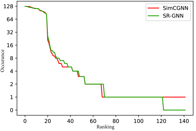
Figure 3: Predicted results of SimCGNN and SR-GNN on sessions with the same last-item (item 33889).

4.7.2 Effect on Solving Popularity Bias

To measure the popularity of recommended items, we calculated Average Recommendation Popularity (ARP) on SR-GNN and SimCGNN to compare the difference in popularity of recommended items between the two methods. The ARP can be calculated as follows,

$$ARP=\frac{1}{|S|}\sum_{s\in S}\frac{\sum_{i\in L_{s}}\phi(i)}{K},$$ (17)

where $\phi(i)$ is the number of times that item $i$ appears in the training dataset, $L_{s}$ is the recommended item list for session $s$, and $S$ is the set of sessions in the test dataset.

From Table 4, it is easy to see that our SimCGNN method has a huge difference in the popularity of recommended items on both datasets compared to SR-GNN. This proves that our method can indeed solve the problem of popularity bias to some extent.

Table 4: SimCGNN versus SR-GNN in terms of Average Recommendation Popularity (ARP). Lower ARP value indicates lower popularity bias.

Method	Yoochoose 1/64	Diginetica
SR-GNN	4128.54	495.25
SimCGNN	2678.64	285.85

5 Conclusion

In this paper, to address the session-based recommendation problem, we proposed a novel Simple Contrastive Graph Neural Network (SimCGNN), which introduces a contrastive module to deal with the ”same last-item confusion” problem and normalized item and session embeddings to cope with popularity bias. Experiments on two real-world datasets validate that our SimCGNN outperforms the state-of-the-art approaches with a significant margin in terms of Recall@20 and MRR@20. In future work, we aim to propose a new combination approach that can eliminate the impact of the last item to a greater extent.

References

- Chang et al. [2015] Shiyu Chang, Wei Han, Jiliang Tang, Guo-Jun Qi, Charu C. Aggarwal, and Thomas S. Huang. Heterogeneous network embedding via deep architectures. In Longbing Cao, Chengqi Zhang, Thorsten Joachims, Geoffrey I. Webb, Dragos D. Margineantu, and Graham Williams, editors, Proceedings of the 21th ACM SIGKDD International Conference on Knowledge Discovery and Data Mining, Sydney, NSW, Australia, August 10-13, 2015, pages 119–128. ACM, 2015.
- Chen et al. [2022] Jinpeng Chen, Yuan Cao, Fan Zhang, Pengfei Sun, and Kaimin Wei. Sequential intention-aware recommender based on user interaction graph. In Vincent Oria, Maria Luisa Sapino, Shin’ichi Satoh, Brigitte Kerhervé, Wen-Huang Cheng, Ichiro Ide, and Vivek K. Singh, editors, ICMR ’22: International Conference on Multimedia Retrieval, Newark, NJ, USA, June 27 - 30, 2022, pages 118–126. ACM, 2022.
- de Souza Pereira Moreira et al. [2021] Gabriel de Souza Pereira Moreira, Sara Rabhi, Jeong Min Lee, Ronay Ak, and Even Oldridge. Transformers4rec: Bridging the gap between NLP and sequential / session-based recommendation. In Humberto Jesús Corona Pampín, Martha A. Larson, Martijn C. Willemsen, Joseph A. Konstan, Julian J. McAuley, Jean Garcia-Gathright, Bouke Huurnink, and Even Oldridge, editors, RecSys ’21: Fifteenth ACM Conference on Recommender Systems, Amsterdam, The Netherlands, 27 September 2021 - 1 October 2021, pages 143–153. ACM, 2021.
- Dong et al. [2020] Yuxiao Dong, Ziniu Hu, Kuansan Wang, Yizhou Sun, and Jie Tang. Heterogeneous network representation learning. In Christian Bessiere, editor, Proceedings of the Twenty-Ninth International Joint Conference on Artificial Intelligence, IJCAI 2020, pages 4861–4867. ijcai.org, 2020.
- Gao et al. [2021] Tianyu Gao, Xingcheng Yao, and Danqi Chen. Simcse: Simple contrastive learning of sentence embeddings. In Marie-Francine Moens, Xuanjing Huang, Lucia Specia, and Scott Wen-tau Yih, editors, Proceedings of the 2021 Conference on Empirical Methods in Natural Language Processing, EMNLP 2021, Virtual Event / Punta Cana, Dominican Republic, 7-11 November, 2021, pages 6894–6910. Association for Computational Linguistics, 2021.
- Gupta et al. [2019] Priyanka Gupta, Diksha Garg, Pankaj Malhotra, Lovekesh Vig, and Gautam Shroff. NISER: normalized item and session representations with graph neural networks. CoRR, abs/1909.04276, 2019.
- He and McAuley [2016] Ruining He and Julian J. McAuley. Fusing similarity models with markov chains for sparse sequential recommendation. In Francesco Bonchi, Josep Domingo-Ferrer, Ricardo Baeza-Yates, Zhi-Hua Zhou, and Xindong Wu, editors, IEEE 16th International Conference on Data Mining, ICDM 2016, December 12-15, 2016, Barcelona, Spain, pages 191–200. IEEE Computer Society, 2016.
- He et al. [2020] Xiangnan He, Kuan Deng, Xiang Wang, Yan Li, Yong-Dong Zhang, and Meng Wang. Lightgcn: Simplifying and powering graph convolution network for recommendation. In Jimmy X. Huang, Yi Chang, Xueqi Cheng, Jaap Kamps, Vanessa Murdock, Ji-Rong Wen, and Yiqun Liu, editors, Proceedings of the 43rd International ACM SIGIR conference on research and development in Information Retrieval, SIGIR 2020, Virtual Event, China, July 25-30, 2020, pages 639–648. ACM, 2020.
- Hidasi et al. [2016] Balázs Hidasi, Alexandros Karatzoglou, Linas Baltrunas, and Domonkos Tikk. Session-based recommendations with recurrent neural networks. In Yoshua Bengio and Yann LeCun, editors, 4th International Conference on Learning Representations, ICLR 2016, San Juan, Puerto Rico, May 2-4, 2016, Conference Track Proceedings, 2016.
- Koren et al. [2009] Yehuda Koren, Robert M. Bell, and Chris Volinsky. Matrix factorization techniques for recommender systems. Computer, 42(8):30–37, 2009.
- Li et al. [2016] Yujia Li, Daniel Tarlow, Marc Brockschmidt, and Richard S. Zemel. Gated graph sequence neural networks. In Yoshua Bengio and Yann LeCun, editors, 4th International Conference on Learning Representations, ICLR 2016, San Juan, Puerto Rico, May 2-4, 2016, Conference Track Proceedings, 2016.
- Li et al. [2017] Jing Li, Pengjie Ren, Zhumin Chen, Zhaochun Ren, Tao Lian, and Jun Ma. Neural attentive session-based recommendation. In Ee-Peng Lim, Marianne Winslett, Mark Sanderson, Ada Wai-Chee Fu, Jimeng Sun, J. Shane Culpepper, Eric Lo, Joyce C. Ho, Debora Donato, Rakesh Agrawal, Yu Zheng, Carlos Castillo, Aixin Sun, Vincent S. Tseng, and Chenliang Li, editors, Proceedings of the 2017 ACM on Conference on Information and Knowledge Management, CIKM 2017, Singapore, November 06 - 10, 2017, pages 1419–1428. ACM, 2017.
- Li et al. [2022] Ansong Li, Zhiyong Cheng, Fan Liu, Zan Gao, Weili Guan, and Yuxin Peng. Disentangled graph neural networks for session-based recommendation. CoRR, abs/2201.03482, 2022.
- Liu et al. [2018] Qiao Liu, Yifu Zeng, Refuoe Mokhosi, and Haibin Zhang. STAMP: short-term attention/memory priority model for session-based recommendation. In Yike Guo and Faisal Farooq, editors, Proceedings of the 24th ACM SIGKDD International Conference on Knowledge Discovery & Data Mining, KDD 2018, London, UK, August 19-23, 2018, pages 1831–1839. ACM, 2018.
- Qiu et al. [2019] Ruihong Qiu, Jingjing Li, Zi Huang, and Hongzhi Yin. Rethinking the item order in session-based recommendation with graph neural networks. pages 579–588, 2019.
- Rendle et al. [2009] Steffen Rendle, Christoph Freudenthaler, Zeno Gantner, and Lars Schmidt-Thieme. BPR: bayesian personalized ranking from implicit feedback. In Jeff A. Bilmes and Andrew Y. Ng, editors, UAI 2009, Proceedings of the Twenty-Fifth Conference on Uncertainty in Artificial Intelligence, Montreal, QC, Canada, June 18-21, 2009, pages 452–461. AUAI Press, 2009.
- Rendle et al. [2010] Steffen Rendle, Christoph Freudenthaler, and Lars Schmidt-Thieme. Factorizing personalized markov chains for next-basket recommendation. In Michael Rappa, Paul Jones, Juliana Freire, and Soumen Chakrabarti, editors, Proceedings of the 19th International Conference on World Wide Web, WWW 2010, Raleigh, North Carolina, USA, April 26-30, 2010, pages 811–820. ACM, 2010.
- Salakhutdinov and Mnih [2007] Ruslan Salakhutdinov and Andriy Mnih. Probabilistic matrix factorization. In John C. Platt, Daphne Koller, Yoram Singer, and Sam T. Roweis, editors, Advances in Neural Information Processing Systems 20, Proceedings of the Twenty-First Annual Conference on Neural Information Processing Systems, Vancouver, British Columbia, Canada, December 3-6, 2007, pages 1257–1264. Curran Associates, Inc., 2007.
- Sarwar et al. [2001a] Badrul Munir Sarwar, George Karypis, Joseph A. Konstan, and John Riedl. Item-based collaborative filtering recommendation algorithms. In Vincent Y. Shen, Nobuo Saito, Michael R. Lyu, and Mary Ellen Zurko, editors, Proceedings of the Tenth International World Wide Web Conference, WWW 10, Hong Kong, China, May 1-5, 2001, pages 285–295. ACM, 2001.
- Sarwar et al. [2001b] Badrul Munir Sarwar, George Karypis, Joseph A. Konstan, and John Riedl. Item-based collaborative filtering recommendation algorithms. In Vincent Y. Shen, Nobuo Saito, Michael R. Lyu, and Mary Ellen Zurko, editors, Proceedings of the Tenth International World Wide Web Conference, WWW 10, Hong Kong, China, May 1-5, 2001, pages 285–295. ACM, 2001.
- Srivastava et al. [2014] Nitish Srivastava, Geoffrey E. Hinton, Alex Krizhevsky, Ilya Sutskever, and Ruslan Salakhutdinov. Dropout: a simple way to prevent neural networks from overfitting. J. Mach. Learn. Res., 15(1):1929–1958, 2014.
- Sun et al. [2019] Fei Sun, Jun Liu, Jian Wu, Changhua Pei, Xiao Lin, Wenwu Ou, and Peng Jiang. Bert4rec: Sequential recommendation with bidirectional encoder representations from transformer. In Wenwu Zhu, Dacheng Tao, Xueqi Cheng, Peng Cui, Elke A. Rundensteiner, David Carmel, Qi He, and Jeffrey Xu Yu, editors, Proceedings of the 28th ACM International Conference on Information and Knowledge Management, CIKM 2019, Beijing, China, November 3-7, 2019, pages 1441–1450. ACM, 2019.
- Tan et al. [2016] Yong Kiam Tan, Xinxing Xu, and Yong Liu. Improved recurrent neural networks for session-based recommendations. In Alexandros Karatzoglou, Balázs Hidasi, Domonkos Tikk, Oren Sar Shalom, Haggai Roitman, Bracha Shapira, and Lior Rokach, editors, Proceedings of the 1st Workshop on Deep Learning for Recommender Systems, DLRS@RecSys 2016, Boston, MA, USA, September 15, 2016, pages 17–22. ACM, 2016.
- Velickovic et al. [2017] Petar Velickovic, Guillem Cucurull, Arantxa Casanova, Adriana Romero, Pietro Liò, and Yoshua Bengio. Graph attention networks. CoRR, abs/1710.10903, 2017.
- Wang et al. [2020] Ziyang Wang, Wei Wei, Gao Cong, Xiao-Li Li, Xianling Mao, and Minghui Qiu. Global context enhanced graph neural networks for session-based recommendation. In Jimmy X. Huang, Yi Chang, Xueqi Cheng, Jaap Kamps, Vanessa Murdock, Ji-Rong Wen, and Yiqun Liu, editors, Proceedings of the 43rd International ACM SIGIR conference on research and development in Information Retrieval, SIGIR 2020, Virtual Event, China, July 25-30, 2020, pages 169–178. ACM, 2020.
- Wu et al. [2018] Zhirong Wu, Yuanjun Xiong, Stella X. Yu, and Dahua Lin. Unsupervised feature learning via non-parametric instance discrimination. In 2018 IEEE Conference on Computer Vision and Pattern Recognition, CVPR 2018, Salt Lake City, UT, USA, June 18-22, 2018, pages 3733–3742. Computer Vision Foundation / IEEE Computer Society, 2018.
- Wu et al. [2019] Shu Wu, Yuyuan Tang, Yanqiao Zhu, Liang Wang, Xing Xie, and Tieniu Tan. Session-based recommendation with graph neural networks. In The Thirty-Third AAAI Conference on Artificial Intelligence, AAAI 2019, The Thirty-First Innovative Applications of Artificial Intelligence Conference, IAAI 2019, The Ninth AAAI Symposium on Educational Advances in Artificial Intelligence, EAAI 2019, Honolulu, Hawaii, USA, January 27 - February 1, 2019, pages 346–353. AAAI Press, 2019.
- Xia et al. [2021] Xin Xia, Hongzhi Yin, Junliang Yu, Qinyong Wang, Lizhen Cui, and Xiangliang Zhang. Self-supervised hypergraph convolutional networks for session-based recommendation. In Thirty-Fifth AAAI Conference on Artificial Intelligence, AAAI 2021, Thirty-Third Conference on Innovative Applications of Artificial Intelligence, IAAI 2021, The Eleventh Symposium on Educational Advances in Artificial Intelligence, EAAI 2021, Virtual Event, February 2-9, 2021, pages 4503–4511. AAAI Press, 2021.
- Xu et al. [2019] Chengfeng Xu, Pengpeng Zhao, Yanchi Liu, Victor S. Sheng, Jiajie Xu, Fuzhen Zhuang, Junhua Fang, and Xiaofang Zhou. Graph contextualized self-attention network for session-based recommendation. In Sarit Kraus, editor, Proceedings of the Twenty-Eighth International Joint Conference on Artificial Intelligence, IJCAI 2019, Macao, China, August 10-16, 2019, pages 3940–3946. ijcai.org, 2019.
- Yu et al. [2020] Feng Yu, Yanqiao Zhu, Qiang Liu, Shu Wu, Liang Wang, and Tieniu Tan. TAGNN: target attentive graph neural networks for session-based recommendation. In Jimmy X. Huang, Yi Chang, Xueqi Cheng, Jaap Kamps, Vanessa Murdock, Ji-Rong Wen, and Yiqun Liu, editors, Proceedings of the 43rd International ACM SIGIR conference on research and development in Information Retrieval, SIGIR 2020, Virtual Event, China, July 25-30, 2020, pages 1921–1924. ACM, 2020.