Cut your Losses with Squentropy

Abstract

Nearly all practical neural models for classification are trained using cross-entropy loss. Yet this ubiquitous choice is supported by little theoretical or empirical evidence. Recent work (Hui & Belkin, 2020) suggests that training using the (rescaled) square loss is often superior in terms of the classification accuracy. In this paper we propose the “squentropy” loss, which is the sum of two terms: the cross-entropy loss and the average square loss over the incorrect classes. We provide an extensive set of experiments on multi-class classification problems showing that the squentropy loss outperforms both the pure cross entropy and rescaled square losses in terms of the classification accuracy. We also demonstrate that it provides significantly better model calibration than either of these alternative losses and, furthermore, has less variance with respect to the random initialization. Additionally, in contrast to the square loss, squentropy loss can typically be trained using exactly the same optimization parameters, including the learning rate, as the standard cross-entropy loss, making it a true “plug-and-play” replacement. Finally, unlike the rescaled square loss, multiclass squentropy contains no parameters that need to be adjusted.

1 Introduction

As with the choice of an optimization algorithm, the choice of loss function is an indispensable ingredient in training neural network models. Yet, while there is extensive theoretical and empirical research into optimization and regularization methods for training deep neural networks (Sun, 2019), far less is known about the selection of loss functions. In recent years, cross-entropy loss has been predominant in training for multi-class classification with modern neural architectures. There is surprisingly little theoretical or empirical evidence in support of this choice. To the contrary, an extensive set of experiments with neural architectures conducted in (Hui & Belkin, 2020) indicated that training with the (rescaled) square loss produces similar or better classification accuracy than cross entropy on most classification tasks. Still, the rescaled square loss proposed in that work requires additional parameters (which must be tuned) when the number of classes is large. Further, the optimization learning rate for the square loss is typically different from that of cross entropy, which precludes the use of square loss as an out-of-the-box replacement.

In this work we propose the “squentropy” loss function for multi-class classification. Squentropy is the sum of two terms: the standard cross-entropy loss and the average square loss over the incorrect classes. Unlike the rescaled square loss, squentropy has no adjustable parameters. Moreover, in most cases, we can simply use the optimal hyperparameters for cross-entropy loss without any additional tuning, making it a true “plug-and-play” replacement for cross-entropy loss.

To show the effectiveness of squentropy, we provide comprehensive experimental results over a broad range of benchmarks with different neural architectures and data from NLP, speech, and computer vision. In 24 out of 34 tasks, squentropy has the best (or tied for best) classification accuracy, in comparison with cross entropy and the rescaled square loss. Furthermore, squentropy has consistently improved calibration, an important measure of how the output values of the neural network match the underlying probability of the labels (Guo et al., 2017). Specifically, in 26 out of 32 tasks for which calibration results can be computed, squentropy is better calibrated than either alternative. We also show results on 121 tabular datasets from (Fernández-Delgado et al., 2014). Compared with cross entropy, squentropy has better test accuracy on 94 out of 121 tasks, and better calibration on 83 datasets. Finally, we show that squentropy is less sensitive to the randomness of the initialization than either of the two alternative losses.

Our empirical evidence suggests that in most settings, squentropy should be the first choice of loss function for multi-class classification via neural networks.

2 The squentropy loss function

The problem we consider here is supervised multi-class classification. We focus on the loss functions for training neural classifiers on this task.

Let $D=(\bm{x}_{i},y_{i})_{i=1}^{n}$ denote the dataset sampled from a joint distribution $\mathcal{D}(\mathcal{X},\mathcal{Y})$. For each sample $i$, $\bm{x}_{i}\in\mathcal{X}$ is the input and $y_{i}\in\mathcal{Y}=\{1,2,\dotsc,C\}$ is the true class label. The one-hot encoding label used for training is $\bm{e}_{y_{i}}=[0,\ldots,\underbrace{1}_{y_{i}},0,\ldots,0]^{T}\in\mathbb{R}^{C}$. Let $f(\bm{x}_{i})\in\mathbb{R}^{C}$ denote the logits (output of last linear layer) of a neural network of input $\bm{x}_{i}$, with components $f_{j}(\bm{x}_{i})$, $j=1,2,\dotsc,C$. Let $p_{i,j}=e^{f_{j}(\bm{x}_{i})}/\sum_{j=1}^{C}e^{f_{j}(\bm{x}_{i})}$ denote the predicted probability of $\bm{x}_{i}$ to be in class $j$. Then the squentropy loss function on a single sample $\bm{x}_{i}$ is defined as follows:

$$l_{\text{sqen}}(\bm{x}_{i},y_{i})=-\log p_{i,y_{i}}(\bm{x}_{i})+\frac{1}{C-1}\sum_{\begin{subarray}{c}j=1,\end{subarray}{j\neq y_{i}}}^{C}f_{j}(\bm{x}_{i})^{2}.$$ (1)

The first term $-\log p_{i,y_{i}}(\bm{x}_{i})$ is simply cross-entropy loss. The second term is the square loss averaged over the incorrect ($j\neq y_{i}$) classes.

The cross-entropy loss is minimized when $f_{y_{i}}(\bm{x}_{i})\to\infty$ while $f_{j}(\bm{x}_{i})\to-\infty$ or at least stays finite for $j\neq y_{i}$. By encouraging all incorrect logits to go to a specific point, namely $0$, it is possible that squentropy yields a more “stable” set of logits — the potential for the incorrect logits to behave chaotically is taken away. In other words, the square loss term plays the role of a regularizer. We discuss this point further in Section 4.2.

Dissecting squentropy.

Cross entropy acts as an effective penalty on the prediction error made for the true class $y_{i}$, as it has high loss and large gradient when $p_{i,y_{i}}$ is close to zero, leading to effective steps in a gradient-based optimization scheme. The “signal” coming from the gradient for the incorrect classes is weaker, so such optimization schemes may be less effective in driving the probabilities for these classes to zero. Squentropy can be viewed as a modification of the rescaled square loss (Hui & Belkin, 2020), in which cross entropy replaces the term $t(f_{y_{i}}(\bm{x}_{i})-M)^{2}$ corresponding to the true class, which depends on two parameters $t$, $M$ that must be tuned. This use of cross entropy dispenses with the additional parameters yet provides an adequate “signal” for the gradient for a term that captures loss on the “true” class.

The second term in (1) pushes all logits $f_{j}(\bm{x}_{i})$ corresponds to false classes $j\neq y_{i}$ to $0$. Cross entropy attains a loss close to zero on term $i$ by sending $f_{y_{i}}(\bm{x}_{i})\to\infty$ and/or $f_{j}(\bm{x}_{i})\to-\infty$ for all $j\neq y_{i}$. By contrast, squentropy “anchors” the incorrect logits at zero (via the second term) while driving $f_{y_{i}}(\bm{x}_{i})\to\infty$ (via the first term). Then the predicted probability of true class $p_{i,y_{i}}(\bm{x}_{i})$ will be close to $\frac{e^{f_{y_{i}}(\bm{x}_{i})}}{e^{f_{y_{i}}(\bm{x}_{i})}+C-1}$ for squentropy, which possibly approaches $1$ more slowly than for cross entropy. When the training process is terminated, the probabilities $p_{i,y_{i}}(\bm{x}_{i})$ tend to be less clustered near $1$ for squentropy than for cross entropy. Confidence in the true class thus tends to be slightly lower in squentropy. We see the same tendency toward lower confidence in the test data, thus helping calibration.

In calibration literature, various post-processing methods, such as Platt scaling (Platt et al., 1999) and temperature scaling (Guo et al., 2017), also improves calibration by reducing $p_{i,y_{i}}$ below $1$, while other methods such as label smoothing (Müller et al., 2019; Liu et al., 2022) and focal loss (Mukhoti et al., 2020) achieve similar reduction on the predicted probability. While all these methods require additional hyperparameters, squentropy does not. We conjecture that calibration of squentropy can be further improved by combining it with these techniques.

Relationship to neural collapse.

Another line of work that motivates our choice of loss function is the concept of neural collapse (Papyan et al., 2020). Results and observations for neural collapse interpose a linear transformation between the outputs of the network (the transformed features $f_{j}(\bm{x}_{i})$) and the loss function. They show broadly that the features collapse to a class average and that, under a cross-entropy loss, the final linear transformation maps them to rays that point in the direction of the corners of the simplex in $\mathbb{R}^{C}$. (A modified version of this claim is proved for square loss in (Han et al., 2021).) Our model is missing the interposing linear transformation, but these observations suggest roughly that cross entropy should drive the true logits $f_{y_{i}}(\bm{x}_{i})$ to $\infty$ while the incorrect logits $f_{j}(\bm{x}_{i})$ for $j\neq y_{i}$ tend to drift toward $-\infty$, as discussed above. As noted earlier, the square loss term in our squentropy loss function encourages $f_{j}(\bm{x}_{i})$ for $j\neq y_{i}$ to be driven to zero instead — a more well defined limit and one that may be achieved without blowing up the weights in the neural network (or by increasing them at a slower rate). In this sense, as mentioned above, the squared loss term is a kind of regularizer.

Confidence calibration.

We use the expected calibration error (ECE) (Naeini et al., 2015) to evaluate confidence calibration performance. It is defined as $\mathbb{E}_{p}[|\mathbb{P}(\hat{y}=y|p)-p|]$, where $p$ and $y$ correspond to the estimated probability and true label of a test sample $\bm{x}$. $\hat{y}$ is the predicted label given by $\operatorname*{arg\,max}_{j}p_{j}$. It captures the expected difference between the accuracy $\mathbb{P}(\hat{y}=y|p)$ and the estimated model confidence $p$. Because we only have finite samples in practice, and because we do not have access to the true confidences $p_{\text{true}}$ for the test set (only the labels $y)$, we need to replace this definition with an approximate ECE. This quantity is calculated by dividing the interval $[0,1]$ of probability predictions into $K$ equally-spaced bins with the $k$-th bin interval to be $(\frac{k-1}{K},\frac{k}{K}]$. Let $B_{k}$ denote the set of test samples $(\bm{x}_{i},\hat{y}_{i})$ for which the confidence $p_{i,y_{i}}$ predicted by the model lies in bin $k$. (The probabilities $p_{i,j}$ are obtained from a softmax on the exponentials of the logits $f_{j}(\bm{x}_{i})$.) The accuracy of this bin is defined to be $\text{acc}(B_{k})=\frac{1}{|B_{k}|}\sum_{i\in B_{k}}\mathbf{1}(\hat{y}_{i}=y_{i})$, where $y_{i}$ is the true label for the test sample $\bm{x}_{i}$ and $\hat{y}_{i}$ is the model prediction for this item (the one for which $p_{i,j}$ are maximized over $j=1,2,\dotsc,C$). The confidence for bin $k$ is defined empirically as $\text{conf}(B_{k})=\frac{1}{|B_{k}|}\sum_{i\in B_{k}}p_{i,y_{i}}$. We then use the following definition of ECE:

$$\text{ECE}=\sum_{k=1}^{K}\frac{|B_{k}|}{n}\left|\text{acc}(B_{k})-\text{conf}(B_{k})\right|.$$ (2)

This quantity is small when the frequency of correct classification over the test set matches the probability of the predicted label.

3 Experiments

In this paper we consider three loss functions, our proposed squentropy, cross entropy and the (rescaled) square loss from (Hui & Belkin, 2020). The latter is formulated as follows:

$${l}_{s}(\bm{x}_{i},y_{i})=\frac{1}{C}\left(t*(f_{y_{i}}(\bm{x}_{i})-M)^{2}+\sum_{j=1,j\neq y_{i}}^{C}f_{j}(\bm{x}_{i})^{2}\right),$$ (3)

where $t$ and $M$ are positive parameters. ($t=M=1$ yields standard square loss.) We will point out those entries in which values $t>1$ or $M>1$ were used; for the others, we set $t=M=1$. Note that following (Hui & Belkin, 2020), the square loss is directly applied to the logits, with no softmax layer in training.

We conduct extensive experiments on various datasets. These include a wide range of well-known benchmarks across NLP, speech, and vision with different neural architectures — more than $30$ tasks altogether. In addition, we evaluate the loss functions on 121 tabular datasets (Fernández-Delgado et al., 2014). In the majority of our experiments, training with squentropy gives best test performance and also consistently better calibration results.

Training scheme.

In most of experiments we train with squentropy with hyperparameter settings that are optimal for cross entropy, given in (Hui & Belkin, 2020). This choice favors cross entropy. This choice also means that switching to squentropy requires a change of just one line of code. Additional gains in performance of squentropy might result from additional tuning, at the cost of more computation in the hyperparameter tuning process.

Table 1: Test performance (perf(%): accuracy for NLP&Vision, error rate for speech data) and calibration: ECE(%).

Domain	Model	Task	Squentropy		Cross-entropy		Square loss
			perf	ECE	perf	ECE	perf	ECE
NLP	fine-tuned BERT (Devlin et al., 2018)	MRPC	84.0	7.9	$82.1$	$13.1$	$83.8$	$14.0$
		SST-2	94.2	$7.0$	$93.9$	6.7	$94.0$	$19.8$
		QNLI	91.0	$7.3$	$90.6$	$7.4$	$90.6$	4.2
		QQP	89.0	2.2	$88.9$	$5.8$	$88.9$	$2.8$
		text5	85.2	12.4	$84.5$	$14.9$	$84.6$	$46.7$
		text20	81.2	10.5	$80.8$	$16.2$	$80.8$	$69.2$
	Transformer-XL (Dai et al., 2019)	text8	$71.5$	3.9	72.8	$5.8$	$73.2$	$57.6$
		enwik8	$77.0$	4.8	77.5	$9.3$	$76.7$	$64.5$
		enwik8 (subset)	48.9	10.7	$48.6$	$18.9$	$47.3$	$70.6$
	LSTM+Attention (Chen et al., 2016)	MRPC	$71.4$	3.2	$70.9$	$7.1$	71.7	$3.5$
		QNLI	79.3	7.2	$79.0$	$7.6$	79.3	$13.0$
		QQP	83.5	2.4	$83.1$	$3.2$	83.4	$16.5$
	LSTM+CNN (He & Lin, 2016)	MRPC	$70.5$	5.2	$69.4$	$6.3$	73.2	$16.3$
		QNLI	76.0	$4.1$	76.0	2.3	76.0	$20.5$
		QQP	84.5	5.1	$84.4$	$7.2$	$84.3$	$24.6$
Speech	Attention+CTC (Kim et al., 2017)	TIMIT (PER)	19.6	0.7	$20.0$	$3.1$	$20.0$	$2.8$
		TIMIT (CER)	32.1	1.6	$33.4$	$3.3$	$32.5$	$4.3$
	VGG+BLSTMP (Moritz et al., 2019)	WSJ (WER)	$5.5$	3.2	$5.3$	$5.0$	5.1	$5.3$
		WSJ (CER)	$2.9$	3.2	$2.5$	$5.0$	2.4	$5.3$
	VGG+BLSTM (Moritz et al., 2019)	Librispeech (WER)	7.6	$7.1$	$8.2$	2.7	$8.0$	$7.9$
		Librispeech (CER)	9.7	$7.1$	$10.6$	2.7	9.7	$7.9$
	Transformer (Watanabe et al., 2018)	WSJ (WER)	3.9	2.1	$4.2$	$4.3$	$4.0$	$4.4$
		Librispeech (WER)	9.1	4.2	$9.2$	$4.9$	$9.4$	$5.1$
Vision	TCNN (Bai et al., 2018)	MNIST	97.8	1.4	$97.7$	$1.6$	$97.7$	$75.0$
	Resnet-18 (He et al., 2016)	CIFAR-10	85.5	8.9	$84.7$	$10.0$	$84.6$	$13.4$
		STL-10	$93.0$	21.2	93.7	$26.1$	$92.5$	$40.3$
	W-Resnet (Zagoruyko & Komodakis, 2016)	CIFAR-100	77.5	10.9	$76.7$	$17.9$	$76.5$	$12.7$
		CIFAR-100 (subset)	43.5	18.8	$41.5$	$40.3$	$41.0$	$23.8$
	Visual transformer	CIFAR-10	99.3	1.9	$99.2$	$3.8$	99.3	$7.2$
	VGG	SVHN	$67.7$	4.8	68.9	$5.7$	$67.0$	$65.4$
	Resnet-50 (He et al., 2016)	ImageNet (acc.)	76.3	6.3	$76.1$	$6.7$	$76.2$	8.2
		ImageNet (Top-5 acc.)	93.2	N/A	$93.0$	N/A	$93.0$	N/A
	EfficientNet (Tan & Le, 2019)	ImageNet (acc.)	$76.4$	$6.8$	77.0	5.6	$74.6$	$7.9$
		ImageNet (Top-5 acc.)	$93.0$	N/A	93.3	N/A	$92.7$	N/A

Datasets.

We test on a wide range of well-known benchmarks from NLP, speech and computer vision. NLP datasets include MRPC, SST-2, QNLI, QQP, text8, enwik8, text5, and text20. Speech datasets include TIMIT, WSJ, and Librispeech. MNIST, CIFAR-10, STL-10 (Coates et al., 2011), CIFAR-100, SVHN (Netzer et al., 2011), and ImageNet are vision tasks. See Appendix A of (Hui & Belkin, 2020) for details of most of those datasets. (The exceptions are SVHN, STL-10, and CIFAR-100, which we describe in Appendix A of this paper). The 121 tabular datasets are from (Fernández-Delgado et al., 2014) and they are mostly small datasets — $90$ of them have $\leq 5000$ samples. The feature dimension is small (mostly $<50$) and most datasets are class-imbalanced.

Architectures and hyperparameter settings.

We choose various modern neural architectures, including simple fully-connected networks, convolutional networks (TCNN(Bai et al., 2018), Resnet-18, VGG, Resnet-50 (He et al., 2016), EfficientNet(Tan & Le, 2019)), LSTM-based networks (Chen et al., 2016) (LSTM+CNN, LSTM+Attention, BLSTM), and Transformers (Vaswani et al., 2017) (fine-tuned BERT, Transformer-XL, Transformer, Visual transformer). See Table 1 for detailed references. We follow the hyperparameter settings given in Appendix B of (Hui & Belkin, 2020) for the cross-entropy loss and the square loss (other than SVHN, STL-10, and CIFAR-100), and use the algorithmic parameters settings of the cross entropy for squentropy in most cases. The exceptions are SVHN and STL-10, where squentropy and square loss have a smaller learning rate (0.1 for cross entropy while 0.02 for squentropy and square loss). More details about hyperparameter settings of SVHN, STL-10, CIFAR-100 are in Appendix B.

Metrics.

For NLP, vision and 121 tabular datasets, we report accuracy as the metric for test performance. For speech dataset, we conduct the automatic speech recognition (ASR) tasks and report test set error rates which are standard metrics for ASR. Precisely, for TIMIT, we report phone error rate (PER) and character error rate (CER). For WSJ and Librispeech, we report CER and word error rate (WER). ECE is the metric to measure the calibration results for all datasets. For speech datasets, we report calibration results for the acoustic modeling part. See Table 1 shows the results of NLP, speech and vision datasets. Figure 2 show results of 121 tabular datasets. In addition, we provide reliability diagrams (DeGroot & Fienberg, 1983; Niculescu-Mizil & Caruana, 2005) to visualize the confidence and accuracy of each interval and see details in Section 3.2.

Remarks on Table 1.

For the results of square loss, we use rescaled square loss with $t>1$ or $M>1$ for TIMIT(PER) ($t=1,M=15$), WSJ ($t=1,M=15$), Librispeech ($t=15,M=30$), CIFAR-10 and CIFAR-100 ($t=1,M=10$), and ImageNet ($t=15,M=30$). All others are the standard square loss. Note that WSJ (WER) and WSJ (CER) share the same ECE number as they share one acoustic model. (Similarly for Librispeech.) Additionally, since ECE numbers are not available for Top-5 accuracy, the corresponding entries (ImageNet, Top-5 acc.) are marked as “N/A”.

For the empirical results reported in Table 1, we discuss generalization / test performance in Section 3.1 and calibration results in Section 3.2. Results for 121 tabular datasets are reported in Section 3.3. We report the average accuracy/error rate (for test performance) and average ECE (for model calibration) of 5 runs with different random initializations for all experiments. We report the standard derivation of this collection of runs in Section 3.4.

3.1 Empirical results on test performance

Figure 1: Confidence histograms (top) and reliability diagrams (bottom) for a Wide Resnet on CIFAR-100. See Table 1 for its test accuracy. The Confidence histogram gives the portion of samples in each confidence interval, and the reliability diagrams show the accuracy as a function of the confidence. The ECE numbers are percentages as in Table 1. Left: Squentropy, Middle left: cross entropy, Middle right: Rescaled square loss, Right: Standard square loss. We see that models trained with squentropy are better calibrated, while cross entropy suffers from overconfidence and the standard square loss is highly underconfident.

Our results show that squentropy has better test performance than cross entropy and square loss in the majority of our experiments. The perf(%) numbers in Table 1 show the test accuracy of benchmarks of the NLP and vision tasks, and error rate for the speech tasks. Squentropy behaves the best in 24 out of 34 tasks. We also report the numbers for subsets of enwik8 and CIFAR-100. Compared with full datasets of these collections, squentropy seems to gain more when the datasets are small.

Applicability and significance.

Table 1 shows improvements for squentropy across a wide range distributions from the NLP, speech, and vision domains. On the other hand, the improvement on one single task often is not significant, and for some datasets, squentropy’s performance is worse. One reason may be our choice to use the optimal hyperparameter values for cross entropy in squentropy. Further tuning of these hyperparameters may yield significant improvements.

3.2 Empirical results on calibration

In this section we show model calibration results, measured with ECE of the models given in Table 1. The ECE numbers for NLP, speech, and vision tasks are also shown in Table 1.

Squentropy consistently improves calibration.

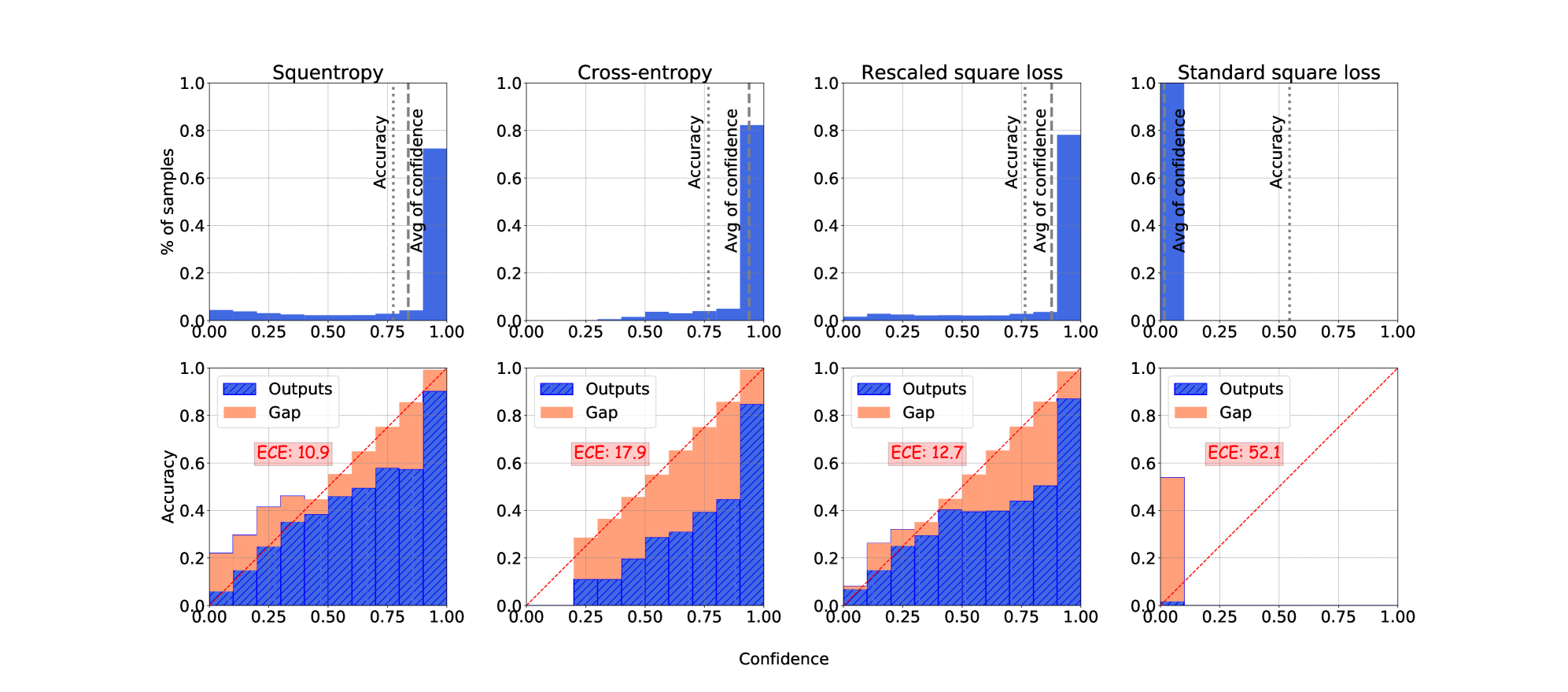
As can be seen in and Table 1, in 26 out of 32 tasks, the calibration error (ECE) of models trained with squentropy is smaller than for cross entropy and square loss, even in those cases in which squentropy had slightly worse test performance, such as WSJ, STL10, and SVHN.

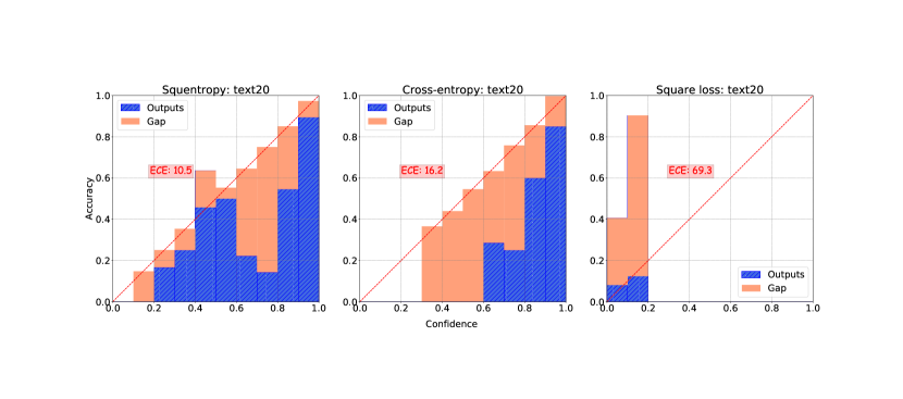
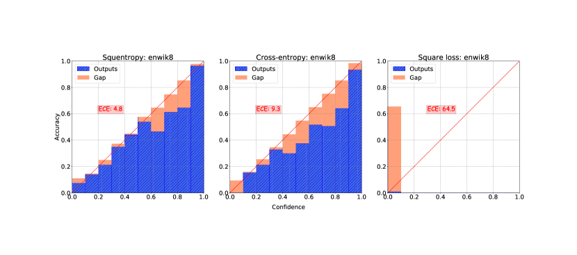
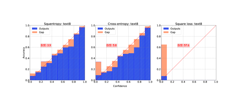
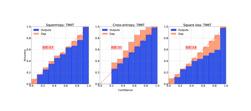
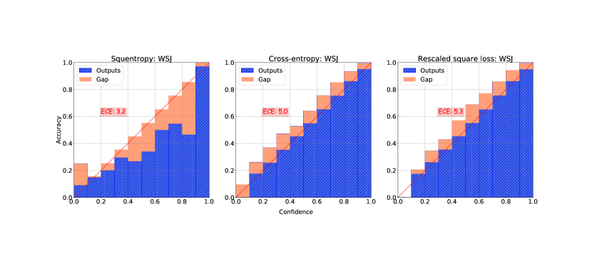
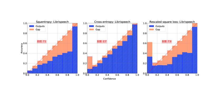
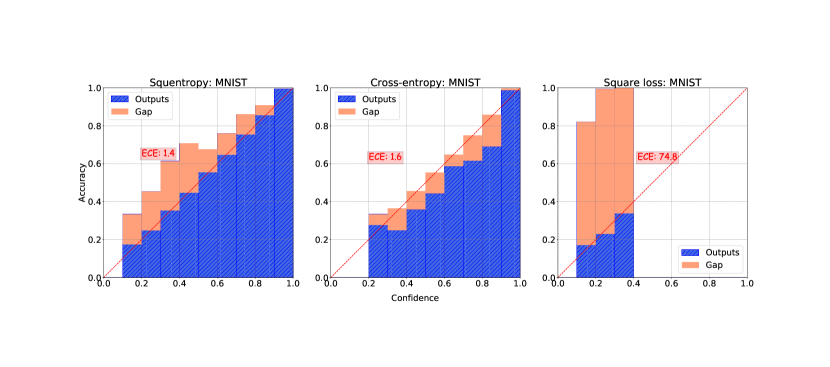
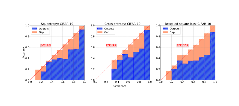
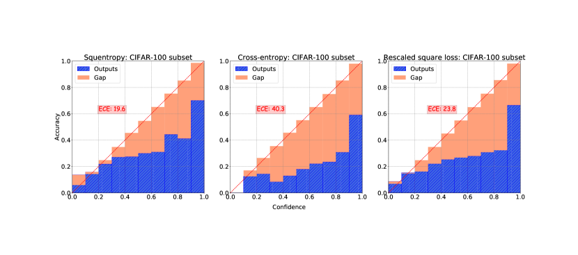
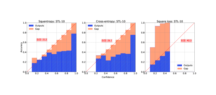
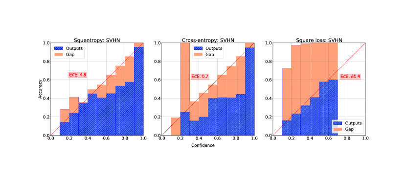
Besides using ECE to measure model calibration, we also provide a popular form of visual representation of model calibration: reliability diagrams (DeGroot & Fienberg, 1983; Niculescu-Mizil & Caruana, 2005), which show accuracy as a function of confidence as a bar chart. If the model is perfectly calibrated, i.e. $\mathbb{P}(\hat{y}_{i}=y_{i}|p_{i})=p_{i}$, the diagram should show all bars aligning with the identity function. If most of the bars lie below the identity function, the model is overconfident as the confidence is mostly larger than corresponding accuracy. When most bars lie above the identity function that means the model is underconfident as confidence is smaller than accuracy. For a given bin $k$, the difference between $\text{acc}(B_{k})$ and $\text{conf}(B_{k})$ represents the calibration gap (orange bars in reliability diagrams – e.g. the bottom row of Figure 1).

In Figure 1 we plot the confidence histogram (top) and the reliability diagrams (bottom) of Wide Resnets on CIFAR-100, trained with four different loss functions: squentropy, cross entropy, rescaled square loss (with $t=1,M=10$), and standard square loss ($t=1,M=1$). The confidence histogram gives the percentage of samples in each confidence interval, while the reliability diagrams show the test accuracy as a function of confidence.

In the reliability diagrams of Figure 1 bottom, the orange bars, which represent the confidence gap, start from the top of the blue (accuracy) bar. We show $\text{conf}(B_{k})-\text{acc}(B_{k})$ for all intervals in all reliability diagram plots. Note that for intervals where confidence is smaller than accuracy, the orange bars go down from the top of the blue bars, such as the one in the right bottom of Figure 1. More reliability diagrams for other tasks are given in Appendix C.

Squentropy vs. cross entropy.

If we compare the diagrams of squentropy and cross entropy, the bars for squentropy are closer to the identity function; cross entropy apparently yields more overconfident models. The gap for squentropy is also smaller than cross entropy in most confidence intervals.

Loss functions	Squentropy	Cross entropy	Square loss
Avg accuracy	85.6%	85.2%	85.5%
Avg ECE	11.6%	13.0%	15.7%

Figure 2: Test accuracy and model calibration of 121 tabular datasets from (Fernández-Delgado et al., 2014) trained with a 3 layer (64-128-64) fully connected network. The results for each dataset are averaged over 5 runs with different random initializations. Left: Test accuracy (larger is better). Right: Calibration error ECE (smaller is better). The top figures plot the results of squentropy and cross entropy, while the bottom figures plot the results of squentropy and the (rescaled) square loss. Test accuracy/ECE for each dataset are tabulated in Appendix D.

Standard square loss leads to underconfidence.

We also plot the reliability diagrams for training with the standard square loss on the right ones of Figure 1. We see that it is highly underconfident as the confidence is smaller than $0.1$ (exact number is $0.017$) for all samples. Note that the square loss is directly applied to the logits $f_{j}(x_{i})$, and the logits are driven to the one-hot vector $\bm{e}_{y_{i}}$, then the probabilities $p_{i,j}$ formed from these logits are not going to be close to the one-hot vector. The “max” probability (confidence) will instead be close to $\frac{e}{e+(C-1)}$, which is small when $C$ is large.

Rescaling helps with calibration.

The second-from-right bottom diagram in Figure 1 shows the results of training with the rescaled square loss ($t=1,M=10$) on CIFAR-100. This minimization problem drives the logits of true class closer to $M$, making the max probability approach $\frac{e^{M}}{e^{M}+(C-1)}$ - a much larger value than for standard square loss, leading to better calibration. However, squentropy can avoid extra rescaling hyperparameters while achieving even smaller values of ECE.

3.3 Additional results on 121 Tabular datasets

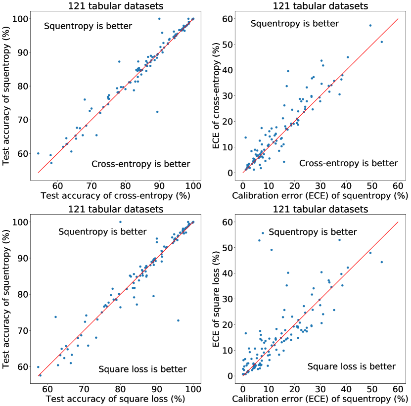
Additional results for 121 small, low dimensional, and class-imbalanced tabular dataset, obtained with 3-layer fully-connected networks, are shown in Figure 2. For all these cases, we use SGD optimizer with weight decay parameter $5*10^{-4}$ and run $400$ epochs with learning rate $0.01$. The “square loss” function used here is in fact rescaled version with parameters $t=1$ and $M=5$.

Figure 2 shows that for most datasets, squentropy has slightly better test accuracy and significantly smaller ECE than cross entropy or square loss. Squentropy has the best test accuracy in 71 out of 121 tasks and best calibration in 60 tasks. If only compare with cross entropy, squentropy is better in 94 tasks on accuracy, and is better on calibration in 83 tasks. Test accuracy and ECE for each dataset in this collection are tabulated in Appendix D.

Table 2: Standard deviation of test accuracy/error. Smaller number is bolded. CE is short for cross-entropy.

Model	Dataset	Squentropy	CE	Square loss
fine-tuned BERT	MRPC	0.285	0.766	0.484
	SST-2	0.144	0.173	0.279
	QNLI	0.189	0.205	0.241
	QQP	0.050	0.063	0.045
	text5	0.132	0.167	0.147
	text20	0.131	0.08	0.172
Transformer-XL	text8	0.149	0.204	0.174
	enwik8	0.156	0.102	0.228
LSTM +Attention	MRPC	0.315	0.786	0.484
	QNLI	0.198	0.371	0.210
	QQP	0.408	0.352	0.566
LSTM +CNN	MRPC	0.289	0.383	0.322
	QNLI	0.154	0.286	0.173
	QQP	0.279	0.161	0.458
Attention +CTC	TIMIT (PER)	0.332	0.249	0.508
	TIMIT (CER)	0.232	0.873	0.361
VGG+ BLSTMP	WSJ (WER)	0.147	0.249	0.184
	WSJ (CER)	0.082	0.118	0.077
VGG+ BLSTM	Libri (WER)	0.117	0.257	0.126
	Libri (CER)	0.125	0.316	0.148
Transformer	WSJ (WER)	0.186	0.276	0.206
	Libri (WER)	0.168	0.232	0.102
TCNN	MNIST	0.151	0.173	0.161
Resnet-18	CIFAR-10	0.147	0.452	0.174
	STL-10	0.413	0.376	0.230
W-ResNet	CIFAR-100	0.164	0.433	0.181
Visual Transformer	CIFAR-10	0.070	0.075	0.063
VGG	SVHN	0.283	0.246	0.307
Resnet-50	I-Net (Top-1)	0.029	0.045	0.032
	I-Net (Top-5)	0.098	0.045	0.126
EfficientNet	I-Net (Top-1)	0.099	0.122	0.138
	I-Net (Top-5)	0.092	0.089	0.089

Figure 3: Decision boundary along different epochs for test samples. We fix all random seeds to be the same for all cases and hence the test set is exactly the same. (Thus, we display legends only in the bottom-row figures). Color coding indicates the calculated probability of class label to be $1$, according to the scale on th eright. The white line between red and blue areas indicates the decision boundary. We train a 3-layer fully connected network with 12 units in each layer, for a 2-class spiral data set in $\mathbb{R}^{2}$. There are 1000 samples for training and 500 samples for test, and we train for 1000 epochs, yielding a training accuracy of $100\%$ for all loss functions. Test accuracies are squentropy: $99.9\%$, cross entropy: $99.7\%$, square loss: $99.8\%$. Top: squentropy. Middle: cross entropy. Bottom: square loss. Columns show results after 100, 500, and 1000 epochs, respectively.

3.4 Robustness to initialization

To evaluate the stability of the model trained with the loss functions considered in this paper, we report the standard deviation of the accuracy/error rate with respect to the randomness in initialization of weights for NLP, speech, and vision tasks. Standard deviation is over 5 runs with different random initializations; see Table 2 for results. The standard derivation of squentropy is smaller in the majority of the tasks considered, so results are comparatively insensitive to model initialization.

4 Observations

As mentioned previously, we conjecture that the square term of squentropy acts as an implicit regularizer and in this section we provide some observations in support of this conjecture. We discuss the decision boundary learnt by a fully-connected network on a 2-class spiral data problem (the “Swiss roll”) in Section 4.1, and remark on the weight norm of the last linear layer of several networks in Section 4.2.

4.1 Predicted probabilities and decision boundary

Using a simple synthetic setting, we observe that the decision boundary learned with squentropy appears to be smoother than that for cross entropy and the square loss. We illustrate this point with a 2-class classification task with spiral data and a 3-layer fully-connected network with parameter $\theta$. This setup enables visual observations. Given a sample $\bm{x}_{i}\in\mathbb{R}^{2}$ and labels $y_{i}\in\{1,2\}$, and the one hot encoding $\bm{y}_{i}=[0,1]$ or $\bm{y}_{i}=[1,0]$, we solve for weights $\theta$ to define functions $f_{1}(\bm{x}_{i})$ and $f_{2}(\bm{x}_{i})$ corresponding to the two classes. For any $\bm{x}_{i}$, we then predict a probability of $\bm{x}_{i}$ being classified as class $1$ as follows: $p(\bm{x}_{i}):=e^{f_{1}(\bm{x}_{i})}/(e^{f_{1}(\bm{x}_{i})}+e^{f_{2}(\bm{x}_{i})})$. Samples are assigned to class $1$ if $f_{i,1}>f_{i,2}$ and to class 2 otherwise. The decision boundary is the set of points for which $\{\bm{x}\,|\,f_{1}(\bm{x})=f_{2}(\bm{x})\}$ or $\{\bm{x}|p(\bm{x}_{i})=1/2\}$.

We see from Figure 3 that the decision boundary obtained with squentropy is smoother than those learnt with both cross entropy and square loss. This appears to be true throughout the training process, on this simple example. Meanwhile, the margin (distance from training points to the decision boundary) is also larger for squentropy in many regions. Together, the large margin and smooth decision boundary imply immunity to perturbations and could be one of the reasons for the improved generalization resulting from the use of squentropy (Elsayed et al., 2018).

Figure 4: Weight norm along training. We train a Resnet-18 on CIFAR-10 (calibration error, ECE: Squentropy: $8.9\%$, cross entropy: $10.0\%$) and STL-10 (ECE: Squentropy: $21.2\%$, cross entropy: $26.1\%$), a wide Resnet on CIFAR-100 (ECE: Squentropy: $10.9\%$, cross entropy: $17.9\%$), and show the norm of the last linear layer’s weights. These are the same experiments as given in Table 1.

4.2 Weight norm

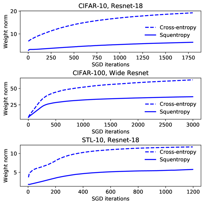
Neural classifiers trained with cross-entropy loss suffer from overconfidence, causing miscalibration of the model (Guo et al., 2017). Our calibration results in Figure 1 and Section C show evidence of this phenomenon. As can be seen in the confidence histogram of cross entropy — the $(1,2)$ figure in Figure 1 — the average confidence $p_{y_{i}}(\bm{x}_{i})$ for the predicted label in cross entropy is close to $1$. This fact suggests that the logits $f_{y_{i}}(\bm{x}_{i})$ of true class are close to $\infty$, while the logits of the incorrect classes approach $-\infty$. Such limits are possible only when the weights of last linear layer have large norm. To quote (Mukhoti et al., 2020), “cross-entropy loss thus inherently induces this tendency of weight magnification in neural network optimisation.”

Guo et al. (2017) comment that weight decay, which corresponds to adding a penalty term to the loss consisting of the sum of squares of the weights, can produce appreciably better calibration while having a minimal effect on test error; see the rightmost diagram in Figure 2 of (Guo et al., 2017). In (Mukhoti et al., 2020; Liu et al., 2022), the authors point out how focal loss proposed in (Lin et al., 2017) improves calibration by encouraging the predicted distribution to have higher entropy, thus implicitly regularizing the weights. Figure C.1 of (Mukhoti et al., 2020) compares weight norm and final logit values between cross entropy and the focal loss, showing that the latter are significantly smaller. We perform a similar experiment, showing in Figure 4 the weight norm of the final-layer weights for three examples from Table 1 as a function of training steps. We observe that the weight norm for the model trained with squentropy is much smaller than the norms for the same set of weights in the model trained with cross entropy, along the whole training process.

5 Summary, thoughts, future investigations

As with the selection of an optimization procedure, the choice of the loss function is an ineluctable aspect of training all modern neural networks. Yet the machine learning community has paid little attention to understanding the properties of loss functions. There is little justification, theoretical or empirical, for the predominance of cross-entropy loss in practice. Recent work  (Hui & Belkin, 2020) showed that the square loss, which is universally used in regression, can perform at least as well as cross entropy in classification. Other works have made similar observations: (Rifkin, 2002; Sangari & Sethares, 2015; Que & Belkin, 2016; Demirkaya et al., 2020). While several alternative loss functions, such as the focal loss (Lin et al., 2017), have been considered in the literature with good results, none have been adopted widely. Even the hinge loss, the former leader in the popularity contest for classification losses, is barely used outside the context of Support Vector Machines.

In this work we demonstrate that a simple hybrid loss function can achieve better accuracy and better calibration than the standard cross entropy on a significant majority of a broad range of classification tasks. Our squentropy loss function has no tunable parameters. Moreover, most of our experiments were conducted in a true “plug-and-play” setting using the same algorithmic parameters in the optimization process as for training with the standard cross-entropy loss. Performance of squentropy can undoubtedly be further improved by tuning the optimization parameters. Furthermore, various calibration techniques can potentially be applied with squentropy in the same way they are used with cross entropy.

Thus, from a practical point of view, squentropy currently appears to be the natural first choice to train neural models.

By no means does it imply that we know of fundamental reasons or compelling intuition indicating that squentropy is the last word on the choice of loss functions for classification. One of the main goals of this work is to encourage both practitioners and theoreticians to investigate the properties of loss functions, an important but largely overlooked aspect of modern Machine Learning.

Appendix A Datasets

Datasets used in our tests include the following.

• CIFAR-100: (Krizhevsky et al., 2009) consists of 50, 000 32×32 pixel training images and 10, 000 32 × 32 pixel test images in 100 different classes. It is a balanced dataset with 6, 00 images of each class.

• SVHN: (Netzer et al., 2011) is a real-world image dataset obtained from house numbers in Google Street View images and it incorporates over 600,000 digit images with labeles. It is a good choice for developing machine learning and object recognition algorithms with minimal requirement on data preprocessing and formatting.

• STL-10: (Coates et al., 2011) is an image recognition dataset mainly for developing unsupervised feature learning as it contains many images without labels. The resolution of this dataset is 96x96 and this makes it a challenging benchmark.

See Appendix A of (Hui & Belkin, 2020) for details of other datasets.

Table 3: Hyper-parameters for CIFAR-100, SVHN, and STL-10.

Model	Task	Hyper-parameters	Epochs training w/
			squentropy	square loss	CE
Wide-ResNet	CIFAR-100	lr=0.1, layer=28 wide-factor=20, batch size: 128	200	200	200
VGG	SVHN	lr=0.1 for cross-entropy lr=0.0.02 for squentropy and square loss	200	200	200
Resnet-18	STL-10	lr=0.1 for cross-entropy for squentropy and square loss lr=0.02	200	200	200

Appendix B Hyperparameters

Detailed hyperparameter settings for CIFAR-100, SVHN, and STL-10 are shown in Table 3. For the other tasks, we follow the exact same settings as provided in Appendix B of (Hui & Belkin, 2020).

Appendix C More reliability diagrams

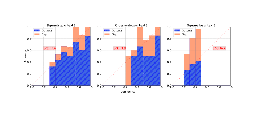
We provide the reliability diagrams for more tasks. Note that the values given for ECE (Expected calibration error as defined in (2) and the smaller the better) in these plots are percentages as in Table 1.

Figure 5: Reliability diagrams for a pretrained BERT on text5 data. Left: squentropy, middle: cross-entropy, right: square loss.

Figure 6: Reliability diagrams for a pretrained BERT on text20 data. Left: squentropy, middle: cross-entropy, right: square loss.

Figure 7: Reliability diagrams for a Transformer-XL on enwik8. Left: squentropy, middle: cross-entropy, right: square loss.

Figure 8: Reliability diagrams for a Transformer-XL on text8. Left: squentropy, middle: cross-entropy, right: square loss.

Figure 9: Reliability diagrams for a Attention+CTC model on TIMIT. Left: squentropy, middle: cross-entropy, right: square loss.

Figure 10: Reliability diagrams for a VGG+BLSTMP model on WSJ. Left: squentropy, middle: cross-entropy, right: scaled square loss.

Figure 11: Reliability diagrams for a VGG+BLSTM model on Librispeech. Left: squentropy, middle: cross-entropy, right: scaled square loss.

Figure 12: Reliability diagrams for a TCN on MNIST. Left: squentropy, middle: cross-entropy, right: square loss.

Figure 13: Reliability diagrams for a Resnet18 on CIFAR-10.Left: squentropy, middle: cross-entropy, right: scaled square loss.

Figure 14: Reliability diagrams for a Wide Resnet on CIFAR-100 subset. Left: squentropy, middle: cross-entropy, right: scaled square loss.

Figure 15: Reliability diagrams for a Resnet18 on STL10. Left: squentropy, middle: cross-entropy, right: square loss.

Figure 16: Reliability diagrams for a VGG on SVHN. Left: squentropy, middle: cross-entropy, right: square loss.

Appendix D Results for 121 tabular datasets

We list the test accuracy and calibration results (ECE) of each tabular dataset in Tables 4, 5 and 6. Note that the square loss of in those tables are all rescaled square loss defined in Equation (3). with $t=1,M=5$.

Table 4: Test accuracy (Acc)/ECE for 121 tabular datasets

Dataset	Squentropy		Cross-entropy		Rescaled square
	Acc	ECE	Acc	ECE	Acc	ECE
abalone	66.0	3.9	67.9	14.1	68.3	13.8
acute-inflammation	96.4	3.8	91.3	4.7	95.8	4.3
acute-nephritis	100.0	1.7	100.0	3.0	100.0	4.8
adult	84.0	4.7	85.1	5.7	85.1	10.7
annealing	94.3	3.6	93.3	3.9	94.4	4.1
arrhythmia	68.1	21.4	67.0	24.5	68.4	17.3
audiology-std	72.6	26.3	73.0	26.0	70.3	29.7
balance-scale	97.2	5.0	96.3	3.8	96.5	4.0
balloons	95.6	23.7	95.4	21.4	90.0	25.8
bank	89.9	4.1	89.8	7.7	89.2	10.6
blood	81.6	11.7	81.9	7.0	81.7	16.6
breast-cancer	76.8	26.6	75.6	24.5	75.5	27.5
breast-cancer-wisc	98.0	4.8	97.6	4.9	97.1	4.5
breast-cancer-wisc-diag	99.5	3.5	99.2	3.4	98.8	2.2
breast-cancer-wisc-prog	89.6	16.3	87.9	15.7	89.0	19.3
breast-tissue	83.3	17.9	84.1	17.1	83.6	19.2
car	100.0	0.4	100.0	0.4	100.0	2.3
cardiotocography-10clases	87.7	6.3	87.8	7.3	87.2	3.9
cardiotocography-3clases	94.8	4.0	94.9	5.5	94.7	4.6
chess-krvk	86.6	3.7	87.8	1.8	86.1	16.0
chess-krvkp	99.8	0.4	99.7	0.5	99.8	0.7
congressional-voting	65.9	9.7	65.7	9.2	65.1	18.3
conn-bench-sonar-mines-rocks	90.6	11.7	91.4	10.2	91.4	13.1
conn-bench-vowel-deterding	99.6	2.7	99.1	1.9	98.9	9.3
connect-4	89.4	3.3	89.0	5.1	89.7	6.6
contrac	57.7	13.6	58.6	30.4	58.0	35.3
credit-approval	89.1	9.4	88.4	11.7	88.6	14.3
cylinder-bands	81.9	13.1	84.1	14.8	83.9	17.8
dermatology	97.6	4.7	97.2	4.4	97.3	3.5
echocardiogram	85.0	17.6	84.9	17.8	84.4	19.3
ecoli	88.2	12.4	88.1	7.8	88.2	9.8
energy-y1	97.3	4.2	97.5	4.2	97.3	3.0
energy-y2	97.2	4.4	96.7	5.3	96.4	4.0
fertility	94.6	23.3	93.4	26.3	90.0	19.4
flags	60.1	27.1	58.4	31.3	57.4	20.6
glass	78.7	18.7	78.1	25.4	78.1	20.8
haberman-survival	80.3	12.2	79.8	17.9	79.7	22.9
hayes-roth	85.8	5.4	84.1	11.4	83.7	13.6
heart-cleveland	62.5	32.0	62.1	32.5	64.6	25.7
heart-hungarian	85.3	17.6	84.8	16.0	85.4	19.2
heart-switzerland	43.8	50.4	43.6	47.7	46.4	44.4
heart-va	42.1	46.0	46.4	54.1	42.0	47.9
hepatitis	77.4	18.1	75.3	20.6	84.5	14.8
hill-valley	66.0	14.2	71.9	36.3	71.1	40.2
horse-colic	85.9	13.3	84.4	13.9	86.0	14.2

Table 5: Test accuracy (Acc)/ECE for 121 tabular datasets

Dataset	Squentropy		Cross-entropy		Rescaled square
	Acc	ECE	Acc	ECE	Acc	ECE
ilpd-indian-liver	77.2	12.7	75.3	22.9	75.9	25.7
image-segmentation	96.8	5.4	94.7	6.5	94.8	6.9
ionosphere	98.3	7.0	98.2	5.5	97.2	6.2
iris	97.2	3.9	97.1	4.3	98.0	2.9
led-display	75.2	10.7	75.3	5.2	74.9	8.3
lenses	76.6	20.8	68.4	21.5	80.0	17.8
letter	98.8	1.1	98.6	1.2	98.4	16.6
libras	93.1	4.9	92.9	5.7	92.5	12.9
low-res-spect	95.9	4.0	95.2	5.0	94.2	7.7
lung-cancer	60.6	27.1	54.7	40.4	62.9	40.4
lymphography	89.2	6.4	87.1	7.1	91.3	8.0
magic	88.3	5.5	89.1	5.3	89.2	8.3
mammographic	81.9	9.4	83.3	8.0	83.4	14.6
miniboone	81.7	20.3	81.5	20.3	77.9	27.2
molec-biol-promoter	87.9	11.4	78.6	9.9	85.5	14.8
molec-biol-splice	87.9	7.1	84.2	10.8	87.2	8.2
monks-1	85.4	14.0	83.6	13.5	87.2	14.6
monks-2	72.9	6.9	89.9	12.8	95.9	14.5
monks-3	93.4	6.7	91.6	7.6	92.0	9.4
mushroom	100.0	0.0	100.0	0.0	100.0	0.7
musk-1	95.2	3.3	94.6	6.3	95.6	4.9
musk-2	100.0	1.1	100.0	0.2	100.0	0.7
nursery	100.0	0.1	100.0	0.0	100.0	2.7
oocytes_merluccius_nucleus_4d	85.1	3.5	86.6	10.4	87.1	14.4
oocytes_merluccius_states_2f	95.4	3.2	95.2	6.3	95.2	4.6
oocytes_trisopterus_nucleus_2f	89.0	5.4	89.7	9.2	89.0	10.7
oocytes_trisopterus_states_5b	97.1	4.3	97.1	4.6	97.3	3.7
optical	99.6	0.9	99.3	1.2	99.0	6.6
ozone	97.7	4.5	97.5	3.9	97.1	3.1
page-blocks	97.7	2.2	97.5	2.3	97.1	1.8
parkinsons	97.0	2.9	97.9	5.8	97.4	4.2
pendigits	99.8	0.2	99.8	0.3	99.9	6.1
pima	79.9	20.8	78.0	22.4	77.4	24.6
pittsburg-bridges-MATERIAL	79.7	15.4	80.4	15.8	89.1	14.0
pittsburg-bridges-REL-L	68.2	30.2	66.2	28.3	73.3	36.5
pittsburg-bridges-SPAN	73.2	31.0	69.9	30.8	73.7	34.6
pittsburg-bridges-T-OR-D	90.1	19.3	90.0	24.5	89.5	17.9
pittsburg-bridges-TYPE	63.4	34.8	63.3	33.0	66.7	39.7
planning	77.9	23.4	75.6	33.5	76.8	31.7
plant-margin	85.1	4.4	84.0	5.9	82.9	55.7
plant-shape	74.3	7.8	73.9	13.9	70.6	49.1
plant-texture	85.3	3.1	84.3	6.2	82.6	52.8
post-operative	73.9	35.2	70.4	34.7	62.2	35.3
primary-tumor	50.0	27.7	49.8	38.5	48.5	24.0
ringnorm	98.6	1.7	98.5	2.1	98.1	1.5

Table 6: Test accuracy (Acc)/ECE for 121 tabular datasets

Dataset	Squentropy		Cross-entropy		Rescaled square
	Acc	ECE	Acc	ECE	Acc	ECE
seeds	100.0	4.0	99.0	6.3	98.6	5.9
semeion	95.4	2.3	94.9	3.5	94.8	10.7
soybean	92.2	3.4	90.8	3.9	91.3	17.5
spambase	95.6	4.1	95.4	4.6	95.0	4.9
spect	76.8	37.3	75.4	41.7	76.2	42.2
spectf	79.3	18.2	82.9	17.1	83.8	21.8
statlog-australian-credit	61.2	24.1	64.5	34.0	66.4	34.1
statlog-german-credit	80.3	15.7	79.1	21.2	79.6	23.1
statlog-heart	86.9	18.0	86.4	15.4	85.9	18.8
statlog-image	99.3	1.4	99.1	1.4	98.8	4.1
statlog-landsat	93.3	5.8	93.0	6.8	92.7	2.7
statlog-shuttle	99.8	0.5	99.8	0.5	99.8	3.7
statlog-vehicle	87.5	7.8	86.9	9.7	86.8	11.9
steel-plates	78.8	9.7	78.5	14.4	78.7	10.2
synthetic-control	99.1	2.1	99.1	2.0	98.7	4.9
teaching	65.1	29.9	63.0	30.5	63.9	37.2
thyroid	98.5	2.0	97.6	2.6	97.9	1.4
tic-tac-toe	99.8	0.3	99.8	0.2	99.8	0.6
titanic	78.6	12.6	78.4	4.2	78.9	13.6
trains	100.0	34.1	90.4	27.2	80.0	53.0
twonorm	98.2	2.0	98.1	2.6	97.7	2.0
vertebral-column-2clases	91.2	8.5	91.1	8.6	91.3	13.1
vertebral-column-3clases	88.0	15.4	86.6	15.1	87.1	16.1
wall-following	96.1	2.2	95.8	3.2	95.7	1.7
waveform	86.5	9.0	86.8	11.2	86.9	12.0
waveform-noise	85.4	9.4	85.4	11.9	86.1	14.1
wine	100.0	3.3	100.0	3.0	100.0	2.9
wine-quality-red	68.8	23.2	68.9	26.6	69.3	19.7
wine-quality-white	65.0	19.9	65.9	25.3	65.5	17.2
yeast	63.3	21.4	63.1	29.9	63.5	18.8
zoo	92.0	4.8	91.9	3.9	91.4	9.1

References

- Bai et al. (2018) Bai, S., Kolter, J. Z., and Koltun, V. An empirical evaluation of generic convolutional and recurrent networks for sequence modeling. arXiv preprint arXiv:1803.01271, 2018.
- Chen et al. (2016) Chen, Q., Zhu, X., Ling, Z., Wei, S., Jiang, H., and Inkpen, D. Enhanced lstm for natural language inference. arXiv preprint arXiv:1609.06038, 2016.
- Coates et al. (2011) Coates, A., Ng, A., and Lee, H. An analysis of single-layer networks in unsupervised feature learning. In Proceedings of the fourteenth international conference on artificial intelligence and statistics, pp. 215–223. JMLR Workshop and Conference Proceedings, 2011.
- Dai et al. (2019) Dai, Z., Yang, Z., Yang, Y., Carbonell, J., Le, Q. V., and Salakhutdinov, R. Transformer-xl: Attentive language models beyond a fixed-length context. arXiv preprint arXiv:1901.02860, 2019.
- DeGroot & Fienberg (1983) DeGroot, M. H. and Fienberg, S. E. The comparison and evaluation of forecasters. Journal of the Royal Statistical Society: Series D (The Statistician), 32(1-2):12–22, 1983.
- Demirkaya et al. (2020) Demirkaya, A., Chen, J., and Oymak, S. Exploring the role of loss functions in multiclass classification. In 2020 54th annual conference on information sciences and systems (ciss), pp. 1–5. IEEE, 2020.
- Devlin et al. (2018) Devlin, J., Chang, M.-W., Lee, K., and Toutanova, K. Bert: Pre-training of deep bidirectional transformers for language understanding. arXiv preprint arXiv:1810.04805, 2018.
- Elsayed et al. (2018) Elsayed, G., Krishnan, D., Mobahi, H., Regan, K., and Bengio, S. Large margin deep networks for classification. Advances in neural information processing systems, 31, 2018.
- Fernández-Delgado et al. (2014) Fernández-Delgado, M., Cernadas, E., Barro, S., and Amorim, D. Do we need hundreds of classifiers to solve real world classification problems? The journal of machine learning research, 15(1):3133–3181, 2014.
- Guo et al. (2017) Guo, C., Pleiss, G., Sun, Y., and Weinberger, K. Q. On calibration of modern neural networks. In International conference on machine learning, pp. 1321–1330. PMLR, 2017.
- Han et al. (2021) Han, X., Papyan, V., and Donoho, D. L. Neural collapse under mse loss: Proximity to and dynamics on the central path. In International Conference on Learning Representations, 2021. arXiv preprint arXiv:2106.02073.
- He & Lin (2016) He, H. and Lin, J. Pairwise word interaction modeling with deep neural networks for semantic similarity measurement. In Proceedings of the 2016 conference of the north American chapter of the Association for Computational Linguistics: human language technologies, pp. 937–948, 2016.
- He et al. (2016) He, K., Zhang, X., Ren, S., and Sun, J. Deep residual learning for image recognition. In Proceedings of the IEEE conference on computer vision and pattern recognition, pp. 770–778, 2016.
- Hui & Belkin (2020) Hui, L. and Belkin, M. Evaluation of neural architectures trained with square loss vs cross-entropy in classification tasks. arXiv preprint arXiv:2006.07322, 2020.
- Kim et al. (2017) Kim, S., Hori, T., and Watanabe, S. Joint ctc-attention based end-to-end speech recognition using multi-task learning. In 2017 IEEE international conference on acoustics, speech and signal processing (ICASSP), pp. 4835–4839. IEEE, 2017.
- Krizhevsky et al. (2009) Krizhevsky, A., Hinton, G., et al. Learning multiple layers of features from tiny images. 2009.
- Lin et al. (2017) Lin, T.-Y., Goyal, P., Girshick, R., He, K., and Dollár, P. Focal loss for dense object detection. In Proceedings of the IEEE international conference on computer vision, pp. 2980–2988, 2017.
- Liu et al. (2022) Liu, B., Ben Ayed, I., Galdran, A., and Dolz, J. The devil is in the margin: Margin-based label smoothing for network calibration. In Proceedings of the IEEE/CVF Conference on Computer Vision and Pattern Recognition, pp. 80–88, 2022.
- Moritz et al. (2019) Moritz, N., Hori, T., and Le Roux, J. Triggered attention for end-to-end speech recognition. In ICASSP 2019-2019 IEEE International Conference on Acoustics, Speech and Signal Processing (ICASSP), pp. 5666–5670. IEEE, 2019.
- Mukhoti et al. (2020) Mukhoti, J., Kulharia, V., Sanyal, A., Golodetz, S., Torr, P., and Dokania, P. Calibrating deep neural networks using focal loss. Advances in Neural Information Processing Systems, 33:15288–15299, 2020.
- Müller et al. (2019) Müller, R., Kornblith, S., and Hinton, G. E. When does label smoothing help? Advances in neural information processing systems, 32, 2019.
- Naeini et al. (2015) Naeini, M. P., Cooper, G., and Hauskrecht, M. Obtaining well calibrated probabilities using bayesian binning. In Proceedings of the AAAI conference on artificial intelligence, volume 29, 2015.
- Netzer et al. (2011) Netzer, Y., Wang, T., Coates, A., Bissacco, A., Wu, B., and Ng, A. Y. Reading digits in natural images with unsupervised feature learning. 2011.
- Niculescu-Mizil & Caruana (2005) Niculescu-Mizil, A. and Caruana, R. Predicting good probabilities with supervised learning. In Proceedings of the 22nd international conference on Machine learning, pp. 625–632, 2005.
- Papyan et al. (2020) Papyan, V., Han, X. Y., and Donoho, D. L. Prevalence of neural collapse during the terminal phase of deep learning training. Proceedings of the National Academy of Sciences, 117(40):24652–24663, 2020. doi: 10.1073/pnas.2015509117. URL https://www.pnas.org/doi/abs/10.1073/pnas.2015509117.
- Platt et al. (1999) Platt, J. et al. Probabilistic outputs for support vector machines and comparisons to regularized likelihood methods. Advances in large margin classifiers, 10(3):61–74, 1999.
- Que & Belkin (2016) Que, Q. and Belkin, M. Back to the future: Radial basis function networks revisited. In Artificial intelligence and statistics, pp. 1375–1383. PMLR, 2016.
- Rifkin (2002) Rifkin, R. M. Everything old is new again: a fresh look at historical approaches in machine learning. PhD thesis, MaSSachuSettS InStitute of Technology, 2002.
- Sangari & Sethares (2015) Sangari, A. and Sethares, W. Convergence analysis of two loss functions in soft-max regression. IEEE Transactions on Signal Processing, 64(5):1280–1288, 2015.
- Sun (2019) Sun, R. Optimization for deep learning: theory and algorithms. arXiv preprint arXiv:1912.08957, 2019.
- Tan & Le (2019) Tan, M. and Le, Q. Efficientnet: Rethinking model scaling for convolutional neural networks. In International conference on machine learning, pp. 6105–6114. PMLR, 2019.
- Towns et al. (2014) Towns, J., Cockerill, T., Dahan, M., Foster, I., Gaither, K., Grimshaw, A., Hazlewood, V., Lathrop, S., Lifka, D., Peterson, G. D., et al. Xsede: Accelerating scientific discovery computing in science & engineering, 16 (5): 62–74, sep 2014. URL https://doi. org/10.1109/mcse, 128, 2014.
- Vaswani et al. (2017) Vaswani, A., Shazeer, N., Parmar, N., Uszkoreit, J., Jones, L., Gomez, A. N., Kaiser, Ł., and Polosukhin, I. Attention is all you need. Advances in neural information processing systems, 30, 2017.
- Watanabe et al. (2018) Watanabe, S., Hori, T., Karita, S., Hayashi, T., Nishitoba, J., Unno, Y., Soplin, N. E. Y., Heymann, J., Wiesner, M., Chen, N., et al. Espnet: End-to-end speech processing toolkit. arXiv preprint arXiv:1804.00015, 2018.
- Zagoruyko & Komodakis (2016) Zagoruyko, S. and Komodakis, N. Wide residual networks. arXiv preprint arXiv:1605.07146, 2016.