YITP-23-07
AdS/BCFT with Brane-Localized Scalar Field
Hiroki Kandaa, Masahide Satoa, Yu-ki Suzukia, Tadashi Takayanagia,b,c and Zixia Weia
aCenter for Gravitational Physics and Quantum Information,
Yukawa Institute for Theoretical Physics, Kyoto University,
Kitashirakawa Oiwakecho, Sakyo-ku, Kyoto 606-8502, Japan
bInamori Research Institute for Science,
620 Suiginya-cho, Shimogyo-ku,
Kyoto 600-8411 Japan
cKavli Institute for the Physics and Mathematics
of the Universe (WPI),
University of Tokyo, Kashiwa, Chiba 277-8582, Japan
In this paper, we study the dynamics of end-of-the-world (EOW) branes in AdS with scalar fields localized on the branes as a new class of gravity duals of CFTs on manifolds with boundaries. This allows us to construct explicit solutions dual to boundary RG flows. We also obtain a variety of annulus-like or cone-like shaped EOW branes, which are not possible without the scalar field. We also present a gravity dual of a CFT on a strip with two different boundary conditions due to the scalar potential, where we find the confinement/deconfinement-like transition as a function of temperature and the scalar potential. Finally, we point out that this phase transition is closely related to the measurement-induced phase transition, via a Wick rotation.
1 Introduction
A boundary conformal field theory (BCFT) is a conformal field theory (CFT) defined on a manifold with boundaries where half of the conformal symmetries are preserved by the boundaries [1, 2, 3, 4]. Gravity duals of boundary conformal field theories (BCFTs) have been actively studied recently as a major generalization of AdS/CFT correspondence [5, 6, 7], so-called the AdS/BCFT [8, 9, 10, 11]. Its bottom-up construction is given by cutting out a part of the bulk AdS surrounded by the end-of-the-world brane (EOW brane). One of the major advantages of AdS/BCFT is that the computation of entanglement entropy in the AdS/BCFT is straightforward, such that the minimal surface in the holographic entanglement entropy [12, 13, 14] can end on the end-of-the-world brane as first noted in [9, 10] (see also [15]). This was recently employed to analyze black hole evaporation processes to derive the Page curve [16], where the Island prescription [17, 18] is expected from the brane-world holography [19, 20, 21, 22, 23, 24, 25, 26, 27, 28, 29, 30, 31]. For further applications of AdS/BCFT to black hole information problem refer to e.g.[32, 33, 34, 35, 36, 37, 38, 39, 40, 41, 42, 43, 44, 45, 46, 47, 48, 49, 50, 51, 52, 53, 54]. There are many other applications of the idea of AdS/BCFT, ranging from quantum many-body aspects of chaotic BCFTs [55, 56, 57, 58, 59, 60, 61, 62, 63, 64, 65, 66, 67, 68, 69, 70, 71, 72, 73] and boundary renormalization group flows [74, 75, 76, 77], to calculating quantum information measures [78, 79, 80, 81, 82, 83, 84, 85, 86] and building cosmological models [87, 88, 89, 90, 91]. The basic duality relations and their consistency of AdS/BCFT have also been analyzed in [92, 93, 94, 95, 96] and string theory realizations have also been studied in [97, 98, 99, 100, 101, 102, 103, 104, 105, 106]. The AdS/BCFT correspondence was generalized in [107, 108, 109, 110, 111, 112] to construct gravity duals with higher codimensions, named wedge holography.
So far, most of the works on the AdS/BCFT have focused on the case where a single conformally invariant boundary is present in a BCFT. The case where a non-conformal boundary is present or the case where different types of boundaries coexist has not been well studied. The main purpose of this paper is to investigate these problems by analyzing a simple variant of the AdS/BCFT where there is a scalar field localized on the end-of-the-world brane. For example, if we consider a string theory embedding of AdS/BCFT with an orientifold as in [10], we can add D-branes on top of the orientifold, which lead to fields localized on the end-of-the-world brane. This single scalar field on the brane is expected to be dual to a boundary primary operator in the BCFT. We also expect that some fields in the bulk AdS can be dynamically localized on the brane and these fields can also be treated as brane-localized fields. Also, a brane-localized scalar field plays an important role in the holographic Kondo effect [113, 57, 58, 114, 115].
Non-trivial profiles of brane-localized scalar fields allow us to construct explicit solutions which describe the boundary RG flows and also those which correspond to the presence of two boundaries with different boundary conditions. This problem was treated in a probe limit in [86] recently. There is another interesting approach to AdS/BCFT with different boundary conditions by introducing a defect on the EOW brane as discussed in [116, 117].
Analytical results are often available in simple constructions of AdS3/BCFT2 with a brane-localized scalar in three dimensions, because the bulk gravity dynamics is still given by the vacuum Einstein equation in three dimensions, whose local solutions are all equivalent to the pure AdS3. We can even design a large number of solutions by tuning the profile of the potential of the scalar field. As we will see in this paper, this allows us to construct explicit boundary RG solutions when the CFT is defined on an upper half plane, a strip, a round disk, and an annulus as we will explicitly see. Moreover, we will be able to find a solution with the end-of-the-world brane which connects two boundaries with different values of the scalar field, which is dual to a BCFT on a strip with two different boundary conditions. In this strip example, we can construct a connected EOW brane solution using the Poincaré AdS3 metric which is not possible without the brane-localized scalar field. We will observe that this solution experiences a phase transition which is analogous to the confinement/deconfinement transition in the presence of chemical potential and temperature. Moreover, we will present a connected EOW brane solution for a BCFT on an annulus for the first time, which is again impossible without the scalar field. In this way, our simple models describe a new broader class of boundary conditions in CFTs, which possess rich structures.
The Wick rotation of the strip example with the scalar field leads to a new time-dependent solution. This can be regarded as a deformation of the solution in [118], which describes a thermalization of a pure state described by a boundary state. In our case with the scalar field, as we will see in this paper, the solution can be more appropriately regarded as the transition matrix instead of a regular quantum state. Accordingly, the holographic entanglement entropy in this class of backgrounds is correctly interpreted as the holographic pseudo entropy. The pseudo entropy is a generalization of entanglement entropy such that it depends on two different quantum states [119]. We will observe that the confinement/deconfinement-like phase transition of the AdS/BCFT with a brane-localized scalar leads to an interesting transition of the time evolution of the entropy from to and then , which looks analogous to the measurement-induced phase transition [120, 121, 122]. Moreover, we will suggest a possibility that our time-dependent gravity dual solution with the EOW brane may be interpreted as a non-unitary evolution such as projection measurements of infrared degrees of freedom with the entanglement entropy showing a measurement-induced phase transition.
This paper is organized as follows. In section two, we present our basic setup of AdS/BCFT with a brane-localized scalar and derive the boundary condition on the end-of-the-world brane. In section three we investigate planar branes in AdSBCFT2 with a scalar field, each of which is dual to either the BCFT with a relevant perturbation on an upper half plane or the BCFT on a strip with a marginal perturbation. In section four, we examine round-shaped branes in AdSBCFT2, dual to BCFTs on annuli or disks with perturbations. In section five, we study higher dimensional examples. In section six, we consider a finite temperature setup in three dimension and analyze the phase transition between the connected and disconnected solution in the presence of the brane-localized scalar field. In section seven we study transition matrices by choosing the time-dependent profile of the brane-localized scalar field which computes the pseudo entropy. We will show that it exhibits an interesting phase transition. In section eight, we draw conclusions and discuss future problems. In appendix A, a detailed analysis of round-shaped EOW brane solutions is presented.
2 AdS/BCFT with brane-localized scalar field
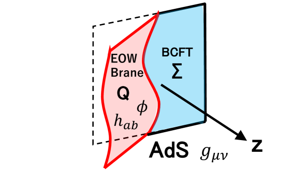
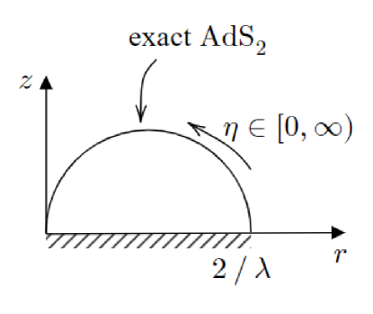
In this section, we present a general formulation of Einstein gravity with a scalar field localized on the end-of-the-world brane (EOW brane) in AdSd+1. This is dual to the -dimensional BCFT on via the AdSBCFTd. The gravity dual is given by the dimensional region whose boundary is given by , as depicted in Fig.1.
This model is described by the total action:
| (2.1) |
where is the bulk metric and is the induced metric on the EOW brane , whose extrinsic curvature is denoted by . On the EOW brane we consider a scalar field as a matter field. The first term is the Einstein-Hilbert action with the cosmological constant and the second one is the Gibbons-Hawking-York term on the asymptotic AdS boundary . By setting the AdS radius to be one, we have . The final term consists of the kinetic term of the scalar field and the potential term in addition to the Gibbons-Hawking term on . If we set and , where is some constant (i.e. the tension of the EOW brane), then this model is reduced to the standard pure gravity model of AdS/BCFT, introduced in [9, 10]. A similar setup with a brane-localized scalar has been analyzed in the context of holographic model Kondo effect [113, 57, 58, 114, 115].
Now, we derive the boundary condition on the EOW brane . This is obtained by varying the action with the bulk equation of motion i.e. the Einstein equation imposed:
| (2.2) |
We obtain the boundary condition by setting the total variation to be vanishing:
| (2.3) |
Particularly, we consider the dynamical gravity on the brane and we choose the following Neumann-type boundary condition:
| (2.4) |
The equation of motion for the scalar field reads
| (2.5) |
It is possible to show that this scalar field equation follows from (2.4) as the right hand side is the energy stress tensor of the scalar field, whose conservation law gives (2.5).
3 AdS3/BCFT2 with planar branes
In this section, we consider a class of AdSBCFT2 setup where the EOW brane takes a planar shape.
We assume the bulk metric is the Poincaré AdS3:
| (3.1) |
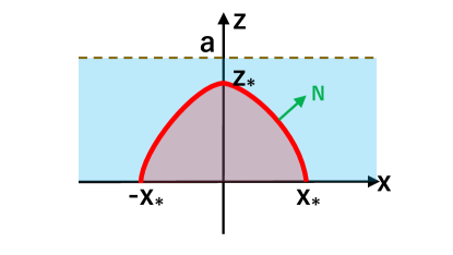
We specify the shape of the EOW brane by
| (3.2) |
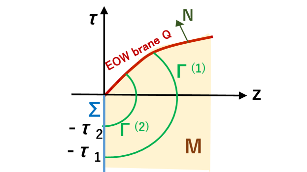
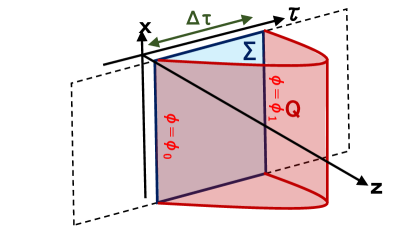
assuming the translationally invariance in the direction. This is depicted in Fig.2. The scalar field also depends on
| (3.3) |
The induced metric reads
| (3.4) |
where we set . The normal vector of the EOW brane reads
| (3.5) |
This leads to the extrinsic curvatures
| (3.6) |
By plugging them into (2.4), the equations are summarized into the following two ones:
| (3.7) | |||
| (3.8) |
Note that for any profile of EOW brane , which satisfies , we can find a solution . This also fixes the form of potential . Thus we can design the potential such that we can obtain a desired solution of the EOW brane.
3.1 Vacuum solution
If we set , then we obtain the standard vacuum solution in AdS/BCFT (see [9, 10]):
| (3.9) |
The entanglement entropy is a useful quantity which characterize the degrees of freedom in BCFTs. The entanglement entropy is defined by the von Neumann entropy for the reduced density matrix , obtained by tracing out the region outside of the subsystem . In AdS/CFT, the entanglement entropy can be computed by the area of minimal area surface which ends on the boundary of the subsystem by
| (3.10) |
In AdS/BCFT, there is one more important aspect: the minimal surface can end on the-end-of-the-world-brane [9, 10, 15].
In Poincaré AdS3, we can easily find that the minimal surface is given by an arc of a circle as shown in Fig.2. If we choose the subsystem to be the interval , then the holographic entanglement entropy reads (we put the UV cut off )
| (3.11) | |||||
where we employed the well-known relation to the central charge of the dual two dimensional CFT: [123]. By comparing with the CFT result [124], the boundary entropy (or the logarithm of the -function) is found to be [9, 10]
| (3.12) |
This vanishes at or equally at and gets divergent at or equally at .
3.2 Boundary RG flow solutions
We expect that the boundary RG will be described as follows: at we have UV fixed point with a tachyon mass , which will flow into the IR fixed point at by a relevant perturbation such that .
At the fixed points, is equal to the tension of the EOW brane and is related to the boundary entropy as in (3.12). We can introduce the boundary entropy (or the logarithm of the -function) in the middle of RG flow by regarding as . This allows us to show the boundary entropy monotonically decreasing as can be derived by noting that is non-negative as required by the equation of motion (3.7). In more general setups, the holographic -theorem was shown in [9, 10] assuming the null energy condition.
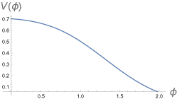
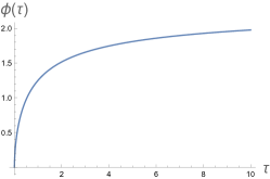
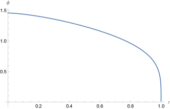
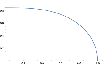
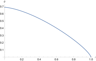
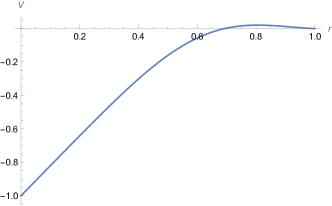
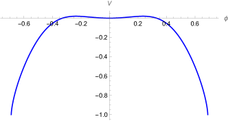
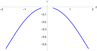
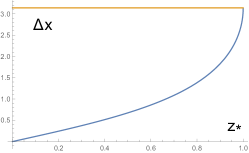
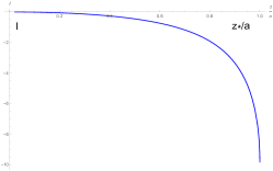
To construct explicit examples of holographic boundary RG flow, we note that we can design the potential such that it solves the equations of motion for a desired profile of as we mentioned before. As the first example, we choose to be
| (3.13) |
This has the UV fixed point at , where , and the IR fixed point is given by the limit , where we have . Note that it satisfies and thus . The potential reads
| (3.14) |
We can find the behavior at :
| (3.15) |
The full plot is shown in Fig.3.
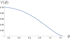
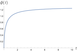
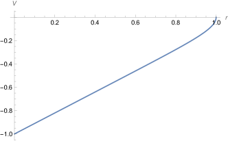
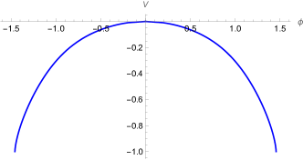
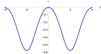
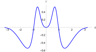
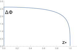
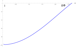
Another example is
| (3.16) |
This also has the UV fixed point at , where , and IR fixed point is also given by the limit , where we have . Again it satisfies and thus . The potential reads
| (3.17) |
we can find the behavior at :
| (3.18) | |||
| (3.19) |
The full plot is shown in Fig.4

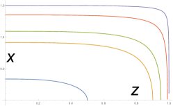
It is also helpful to evaluate the holographic entanglement entropy. We choose subsystem as an interval and the coordinates of two endpoints of the interval as
| (3.20) |
By increasing the value of , we can probe from UV to IR degrees of freedom. Thus the flow of is interpreted as the RG flow.
To calculate the entanglement entropy, we would like to identify the geodesic which ends on the EOW brane. So we write the endpoint on the brane as . Because of the symmetry of the interval under , it is sufficient to assume that the surface begins from and ends on the EOW brane (refer to Fig.2). It is helpful to embed Euclidean AdS3 spacetime in -dimensional Minkowski space
| (3.21) |
with the following embedding equation
| (3.22) |
where satisfies
| (3.23) |
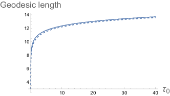
By using this embedding, we can evaluate geodesic length between and as
| (3.24) |
where and are embedding of and respectively. By using this formula, we get the geodesic length between P and the EOW brane
| (3.25) |
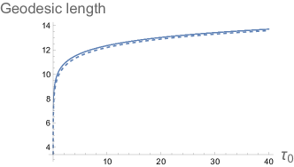
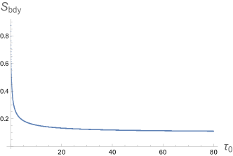
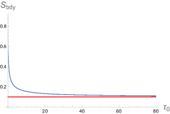
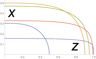
In order to find the minimum value of the quantity above, we need to minimize the first term in the bracket. After choosing the profile , the -dependent term can be minimized by a numerical calculation and we can evaluate the behavior of boundary entropy by subtracting from the minimum geodesic length. We chose the two different cases: and and study their behaviors (we set ). In the case , since we have , in the UV limit , the boundary entropy takes the value . On the other hand, in the IR limit we find . We can confirm this from the plot in right panel of Fig.5. Similarly, in the case , boundary entropy should satisfy and in the UV and IR limit, respectively. Again we can confirm these from the right panel of Fig.6. These behaviors are consistent with the -theorem.
3.3 BCFT on a strip
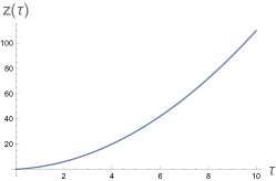
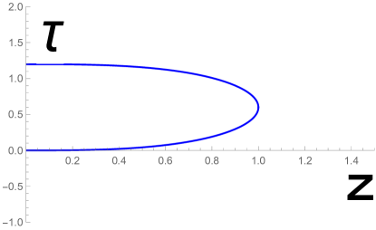
Now we turn to the AdSBCFT2 setup which is dual to a BCFT on a strip . In this case, assuming that the EOW brane is a connected surface, takes a half cylinder shape as depicted in Fig.7. We again assume the translational invariance along and write the profile of as . Choosing the sign convention of the normal vector as , we obtain the following equation of motion
| (3.26) |
By eliminating , we obtain
| (3.27) |
For simplicity, we set , i.e. the massless scalar and zero tension. In this case we have , which is solved by setting , leading to . In the end we find that is obatined by solving
| (3.28) |
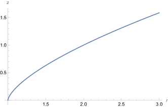
where is an integration constant which gives the turning point. We obtain
| (3.29) |
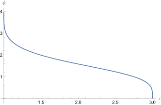
Near , they behave like
| (3.30) |
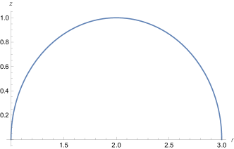
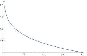
We write the two end points as and . The full solution of is plotted in Fig.9.
It is also easy to estimate the shift:
| (3.31) |
It is also intriguing to note that dependence of on , which is asymptotically AdS2, agrees with the standard asymptotic behavior of scalar field dual to a marginal deformation:
| (3.32) |
in the boundary limit . Here, is the marginal boundary primary operator in the BCFT and is its source. This agrees with the standard dictionary of AdS/CFT [6, 7, 127]. It is intriguing to remember that without any scalar field, a connected solution dual to the BCFT on a strip is not available in the Poincaré AdS3 but is only possible in the thermal AdS3 geometry. In the presence of brane-localized scalar, we are able to construct such a solution in the Poincaré AdS3. Even though we only constructed the solution with a special value of , solutions for other values of will be constructed in section 6, using either the thermal AdS3 or BTZ spacetime.
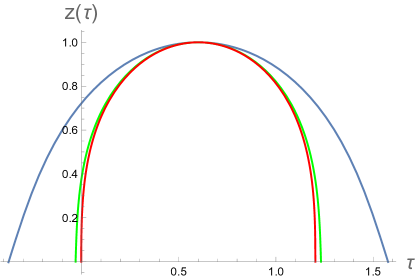
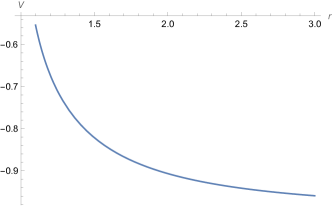
Even if we set , we can get similar profile of . For example, in case of , behaves like the figure below and their end point and beginning point on the boundary changes with respect to the value of .
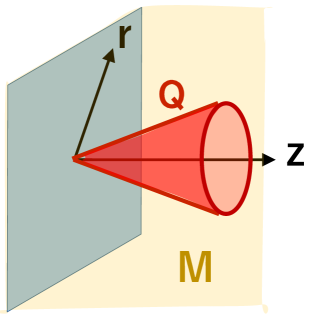
4 AdS3/BCFT2 with round-shaped branes
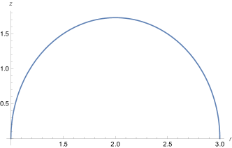
Here we consider the AdSBCFT2 setup with round shaped branes as depicted in Fig.10. For this, we introduce the polar coordinate of Poincaré AdS3:
| (4.1) |
We consider the EOW brane with the rotational invariant profile
| (4.2) |
The induced metric reads
| (4.3) |
where we set . The normal vector of the EOW brane reads
| (4.4) |
This leads to
| (4.5) |
The full equations of motion (2.4) are summarized into
| (4.6) |
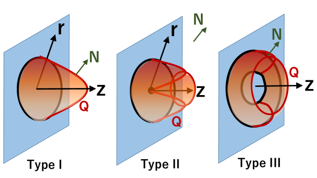
4.1 Type I, Hemisphere-like shaped brane
The boundary conditions of Type I are
| (4.7) |
The third condition demands the brane intersect with the asymptotic boundary. Solving will impose restrictions on :
| (4.8) |
where is an arbitrary function satisfying and on , and is an intersection point of the brane and the asymptotic boundary. In particular, when is constant and , this solution reproduces the well-known hemispherical brane with constant tension and without matter fields. The solution (4.8) is an improvement of this hemispherical brane. A more detailed derivation is summarized in the Appendix A.
Try to stretch or compress the obtained solutions. In other words, when is a solution of (4.7), we find conditions in for which also becomes solution. Then there exists a satisfying the following
| (4.9) |
Therefore, has an upper bound
| (4.10) |
For example, when is constant, we cannot stretch spheres and only oblate spheres () are allowed.
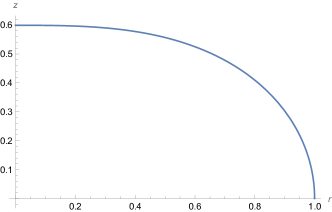
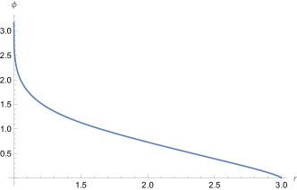
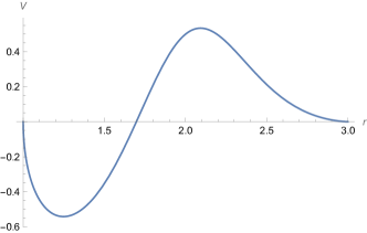
Calculate the mass of the scalar field on brane and the conformal dimension of corresponding boundary operator when and . is determined so that . As the result, is complicated function expressed using a hypergeometric function. The numerical profile of this configuration is summarized in Fig.11.
Obviously, the induced metric (4.3) is not exact Poincaré, but coordinate transformation tells that this is asymptotic AdS2. Actually, since, near the asymptotic boundary , is expanded by as
| (4.11) |
the induced metric can be read
| (4.12) |
In this coordinate, the behavior of is
| (4.13) |
and conformal dimension of corresponding boundary operator reads as . This implies the mass of is and is consistent with the coefficient of potential . Therefore, we can conclude this deformation is relevant.
As before, by introducing new coordinate , we can get asymptotically AdS2 induced metric. At this time Near the asymptotic boundary, behaves as follows:
| (4.14) |
Hence, we can read and , and they match the result from potential, but this is irrelevant because .
However, when is slightly less than , e.g., , the result is
| (4.15) |
and this is a relevant perturbation. Namely, serves as the threshold between relevant and irrelevant deformation.
4.2 Type II, Cone-like shaped brane
In this and next subsections, analyses similar to those in the previous subsection will be performed for different configurations Type II and III.
The boundary conditions of Type II are
| (4.16) |
This solution is
| (4.17) |
where controls the gradient and is arbitrary function satisfying
| (4.18) |
When , we can find a conical solution (Fig.13):
| (4.19) |
In this case, the induced metric
| (4.20) |
is not asymptotically AdS2, but conformally flat because, by ,
| (4.21) |
This means conical solution is not made by any boundary perturbations.
We see another example with and . After some calculation, we get a configuration:
| (4.22) |
This brane is half of a torus whose minor radius is 0, and and diverge at .
A geometry on this brane is exactly AdS2 because the induced metric
| (4.23) |
can be changed into
| (4.24) |
by coordinates changing
| (4.25) |
This means , corresponding to , is an asymptotic boundary of the brane but is deep interior.
Only for the boundary , we can apply calculation of conformal dimension of . Near the asymptotic boundary of the brane,
| (4.26) |
This means that the conformal dimension of the dual scalar operator is and the mass of the scalar field is .
4.3 Type III, Annulus-like shaped brane
The boundary conditions of the third case is
| (4.27) |
The Solution is
| (4.28) |
and satisfies
| (4.29) |
For example, and passes this conditions, the corresponding configuration is given by
| (4.30) |
or a half of torus whose minor radius is and major radius is .
This brane has two asymptotic boundaries. As in Type I, new coordinate is introduced as follows:
| (4.31) |
Near , we choose negative sign, on the other hand, near , positive sign. Then induced metric for both boundaries becomes
| (4.32) |
can also be expanded, for one boundary ,
| (4.33) |
and, for the other boundary ,
| (4.34) |
where we ignore constant shift of . Therefore dimension of dual operator is and mass of scalar field is . This type of configuration is dual of Janus solution.
By similar analysis in Type I, we can find that this configuration can be stretched by . When , at , conformal weight is , but, at , (Fig.16). Hence, only the boundary at is irrelevant. Furthermore, for example, when , corresponding boundary RG flows are relevant for both boundary.
Next, we consider the case where brane does not intersect with the asymptotic boundary in . We find that any function satisfying , and is a special solution of (4.27) because meets (4.29).
In the following we list the results for two example and .
the former is an example where AdS2 radius of asymptotic boundary of brane is . The potential can be displayed analytically using as follows:
| (4.35) |
Then the induced metric is
| (4.36) |
where . Namely, the geometry of this brane is asymptotically AdS2 with radius and
| (4.37) |
Therefore conformal weight is consistent since
| (4.38) |
In this way, the gradient of at asymptotic boundary changes the boundary AdS radius .
The latter is an example of . Actually, the profile Fig.17 are
| (4.39) |
and we can read , , and . Of course, these satisfy the relation .
4.4 Holographic entanglement entropy
In this subsection, we calculate the entanglement entropy in this polar system in similar way as the previous chapter.
The geodesic length (3.24) of AdS in polar coordinates is
| (4.40) |
where is a point in dual BCFT region and is a point of the brane. Obviously, to minimize this length implies . The derivative with respect to yields
| (4.41) |
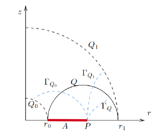
Specially, we calculate the entropy when the dual BCFT region is annulus and subregion is a interval , i.e., like Fig.18. Also, the geodesic connecting and brane is denoted as . If BCFT has no boundary perturbation, the shape of the brane is an exact hemisphere. Therefore, the entropy change of this RG flow is computed by
| (4.42) |
For the branes and , solving (4.41), we obtain
| (4.43) |
Hence, for example, when the brane is simply , , and , we find
| (4.44) |
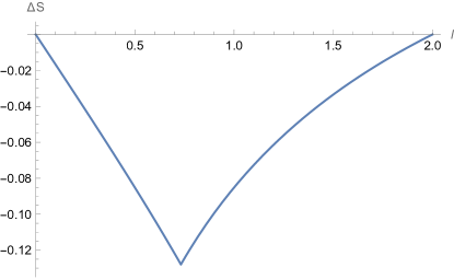
As we can see in Fig.19, vanishes at and decreases as the brane flows to deep interior. These mean also that the corresponding RG flow is relevant.
4.5 Boundary entropy in the presence of brane-localized scalar
In this section, we calculate boundary entropy for simple case. Consider a case where BCFT region is and brane is . If , brane is a tension-less and has no matter part. Therefore, the boundary entropy can be calculated by , where
| (4.45) |
and is gravitational dual region. After some calculation, we get
| (4.46) |
Since this integral diverges, we introduce cutoff . Then the integral have finite value
| (4.47) |
Finally the boundary entropy is
| (4.48) |
5 Analysis of higher dimensional AdS/BCFT
Next we consider extensions of the results in previous sections to higher dimensional AdS/BCFT setups.
5.1 Planar branes
We assume the bulk metric is Poincaré AdSd+1:
| (5.1) |
We specify the shape of the EOW brane and the brane-localized scalar field on by
| (5.2) |
The induced metric on reads
| (5.3) |
The normal vector of the EOW brane is
| (5.4) |
Then, the extrinsic curvature satisfies
| (5.5) | |||
| (5.6) |
By plugging them into(2.4), we get
| (5.7) | |||
| (5.8) |
By eliminating from , we can express as
| (5.9) |
We consider case and then we get .We can solve this equation by setting . Then reads to
| (5.10) |
By solving this equation, we finally find
| (5.11) |
where is an integration constant i.e. the value of of turning point. According to this, we have
| (5.12) | |||
| (5.13) |
Around , these behave as
| (5.14) | |||
| (5.15) |
Near , the geometry is approximated by AdS d
| (5.16) |
and dependence of agrees with the marginal deformation in the standard dictionary of AdS/CFT [6, 7, 127].
It is also useful to evaluate the on-shell action namely the free energy as an exercise of our later analysis of phase transition in section 6. The total action is given by in (2.1), namely,
where we added the counter term .
We would like to evaluate the on-shell action for the solution (5.11) and (5.13) with the UV cut off . We note that the extrinsic curvature takes the value on and . Then the action is evaluated as follows:
| (5.17) | |||||
where the counter term removes all divergent terms proportional to . In this way, we find that the total action or free energy vanishes. In section 6, we will extend this analysis at zero temperature to that at finite temperature to study phase transitions, focusing on the case.
5.2 Round-shaped branes
The polar AdSd+1 metric is
| (5.18) |
where is a metric of . We assume the shape of EOW brane and the scalar field depends on
| (5.19) |
The induced metric reads
| (5.20) |
The normal vector of the EOW brane is
| (5.21) |
Then, we get
| (5.22) | |||
| (5.23) |
By combining (2.4) with them,we get
| (5.24) | |||
| (5.25) |
and the expression of does not depend on the dimension . Because the shape of brane is determined by the positivity condition of in polar case, we can apply the same discussion as and only the mass and the conformal dimension are modified by potential.
6 AdS3/BCFT2 with brane-localized scalar at finite temperature and phase transition
In the standard AdS/CFT, we expect the Hawking-Page phase transition from the thermal AdS phase to AdS black hole phase as we increase the temperature [128, 7, 129], which is interpreted as the confinement/deconfinement phase transition. In the AdS/BCFT, an analogous phase transition was found in [9, 10] for AdSBCFT2 without any matter fields. The purpose of this section is to extend this analysis to AdSBCFT2 with a brane-localized scalar field. We will set the potential to zero . Thus we have a massless scalar on the EOW brane.
The BCFT2 is defined on a cylinder, which is described by the coordinate such that
| (6.1) |
where is the width of the cylinder and is the inverse temperature. See the left panel of Fig.20 for a sketch. This is dual to a region surrounded by the EOW brane whose profile is specified by , assuming the translational invariance in the Euclidean time direction. There are two candidates of the bulk metric, namely the thermal AdS3 and the BTZ metric.111 One may wonder if other bulks solutions give the brane solutions with the required boundary condition. However, this is not possible and we do not need to worry this. This is shown as follows. The general bulk solution to the vacuum Einstein equation with a negative cosmological constant is characterized by energy flux and as in the Banados’s solution [130, 131]. However, here we require the translation invariance in the time direction as we are interested in a static AdS/BCFT setup. Then the energy flux should take a constant value. Thus this leads to either thermal AdS or BTZ, depending on whether the energy density is positive or negative. In addition we turn on the massless scalar field on the EOW brane, whose configuration is expressed as . Below we write the derivative of w.r.t as .
In this model, the only input parameters are two dimensionless quantities: the temperature times the width and the difference of the scalar field
| (6.2) |
owing to the conformal invariance. Once these two values are given, we can find a unique solution which satisfies the equation of motion and the boundary condition in the AdS/BCFT. In case we have multiple solutions we pick up the one with the smallest free energy. Below we will study the thermal AdS3 solution and the BTZ one in detail. Then we will work out the phase structure for non-zero and .
6.1 Thermal AdS3 Solution
Consider the thermal AdS3 solution:
| (6.3) |
In the absence of EOW brane, we need to compactify the coordinate such that to avoid the conical singularity. However, in AdS/BCFT, we do not need to worry about the singularity if it is outside of the considered region surrounded by the EOW brane. Notice also that in the absence of the brane-localized scalar, the Neumann boundary condition fixes the width of the interval to be [9, 10]. However this is no longer true in our model when the scalar field is turned on.
The normal vector of EOW brane reads
| (6.5) |
The Neumann boundary condition (2.4) leads to
| (6.6) |
In our brane profile we can calculation the extrinsic curvature as follows:
| (6.7) |
where .
6.1.1 Analysis of Thermal AdS3 at
By setting , we find
| (6.8) |
We can rewrite this as follows
| (6.9) |
where notice again that and mean and , respectively.
Now, we introduce which is related to via
| (6.10) |
This is solved in terms of as
| (6.11) |
Note that behaves as follows
| (6.12) |
The function satisfies the following equation of motion when we regard as the time:
| (6.13) |
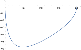
where we introduced the potential energy . This potential is given in terms of as
| (6.14) |
which is a function of via (6.11). It behaves like
| (6.15) |
The energy conservation leads to
| (6.16) |
where is the turning point of the trajectory. The EOW brane is described by such that at we have and at we have .
Thus and are obtained by solving the first order differential equations
| (6.17) |
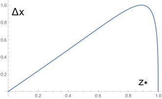
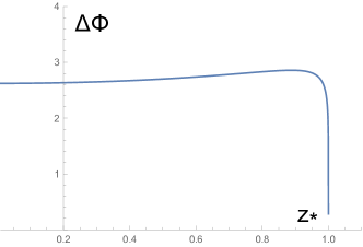
In Fig.21, we plotted the value of the width and the shift of scalar field as function of at . Note that takes the values in the range and that the limit (or equally ) reproduces the previous results for the Poincaré AdS3 in section 3.3. Indeed, we can confirm (3.31) in the limit, which is rewritten as and in the present notation. Also notice that in the opposite limit , the solution is reduced to the known standard one [9, 10] without any scalar field, which means . Also refer to Fig.22 for the plots of the brane profile .
Now, we consider how we can find solution when the width , the temperature and the strength of the external field are given.
In our thermal AdS brane solution, the temperature i.e. periodicity of is arbitrary. The integral of (6.17) leads to the relation
| (6.18) |
where the functions and are given by Fig.21. Therefore, for a given , we find and then for a given , is determined. In this way, we can fully fix the solution. This implies that there is an upper bound of . This argument also shows that the independent input parameters are the two dimensionless quantities (6.2), as expected from the conformal symmetry of this system. Note that we have
| (6.19) |
where agrees with (3.31).222It is intriguing to note that is always less than i.e. . In the standard case without any matter field on the EOW brane, we have , which means that the EOW brane covers the precisely semi-circle of the AdS boundary. In the presence of brane-localized scalar, the above results shows that it only covers less than a half of the boundary circle. This prohibits a construction of traversable wormhole in the present AdS/BCFT setup, providing a consistency check of our model.
6.1.2 Free Energy in Thermal AdS3
Now we would like to evaluate the free energy at a fixed temperature , which is given by the on-shell action (2.1) itself, using our solution in thermal AdS3. The total on-shell action, written by , is given by
| (6.20) |
where is the local counter term which subtract divergence for the standard geometric cut off . Note that since we set , the boundary condition (2.4) leads to . We compactify the Euclidean time direction as . we write the bulk 3d space by i.e. the region , which is surrounded by the AdS boundary and the EOW brane . We also note
| (6.21) |
We have to be careful when we subtract the counter term. The counter term corresponds to the contribution of Poincaré AdS3 i.e. the metric with . However, we need to adjust the length of interval in direction [128] such that
| (6.22) |
where is the length of the interval in the Poincaré Ad33, while is the original one in thermal AdS3.
is explicitly given by the gravity action on the Poincaré AdS3 with the two parallel EOW brane :
| (6.23) | |||||
Thus, the boundary term on cancels completely as usual in AdS:
| (6.24) |
Now we can evaluate the on-shell action in the thermal AdS3 with the EOW brane as follows
| (6.25) |
where we employed the differential equation (6.17) many times. It is useful to note that we can write the free energy (6.25) as follows
| (6.26) |
such that it only depends on the two input parameters (6.2). This is plotted in the left panel of Fig.23.
6.2 Connected EOW brane in BTZ
Now, we consider a connected EOW brane in the BTZ black hole solution:
| (6.28) |
The induced metric on a EOW brane reads
| (6.29) |
Using the normal vector of EOW brane
| (6.30) |
we find the Neumann boundary condition (2.4) explicitly
| (6.31) |
In our setup, we have
| (6.32) |
where .
6.2.1 Analysis of BTZ at
By setting , we obtain
| (6.33) |
We can rewrite this as follows
| (6.34) |
where notice again that and mean and , respectively.
Introduce a new function , related to via
| (6.35) |
which is solved in terms of as
| (6.36) |
It is helpful to notice that behaves as
| (6.37) |
The function satisfies
| (6.38) |
where we introduced the potential energy . This potential is given in terms of as
| (6.39) |
which is the same as that in thermal AdS3. As a function of via (6.36), this behaves like
| (6.40) |
The energy conservation leads to
| (6.41) |
where is the turning point of the trajectory. The EOW brane is described by such that at we have and at we have .
Thus and are obtained by solving the first order differential equations
| (6.42) |
In Fig.24, we showed the value of the width and the shift of scalar field as function of at . Note that takes the values in the range and that the limit reproduces the previous results for the Poincaré AdS3 in section 3.3. Also notice that in the limit , the solution is reduced to the know standard one without any scalar field i.e. the disconnected vertical solution and . Refer to Fig.25 for the plots of the brane profile.
In our BTZ solution, the temperature i.e. periodicity of is arbitrary, assuming . If , then we consider the disconnected solution where the temperature is fixed as as usual. The integral of (6.42) leads to the relation
| (6.43) |
where the functions and are given by Fig.24. Therefore, for a given , we find and then the given fixes the value of . In this way we can fully fixes the solution once the two input parameters (6.2) are given. However, we will see shortly below, the connected EOW brane solution in BTZ is never favored as it has a larger free energy.
6.2.2 Free Energy for a connected EOW brane in BTZ
Now we would like to evaluate the gravity action to calculate the free energy (6.20) for our on-shell solution in BTZ with the EOW brane, which is written as . When we subtract the Poincaré AdS3 solution as the counter term, we need to rescale the inverse temperature as follows
| (6.44) |
where is the periodicity of in the Poincaré AdS3, while is the original one in BTZ.
The counter term is explicitly given by the gravity action on the Poincaré AdS3 with the two parallel EOW branes :
| (6.45) | |||||
Thus, the boundary term on cancels completely as usual in AdS:
| (6.46) |
Now we can evaluate the on-shell action in the BTZ with the EOW brane as follows
| (6.47) |
This shows that . We have in the limit i.e. when the solution approaches the one in the Poincaré AdS3. This agrees with our previous result (5.17). Also in the opposite limit we find . However, since , this connected solution in BTZ will not be favored thermodynamically.
6.3 Disconnected EOW Solution in BTZ
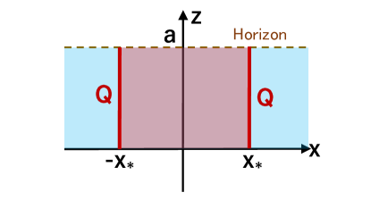
It is important to note that there is another solution of EOW branes in BTZ even when . This is the solution with two disconnected EOW branes as sketched in Fig.26. This is given by setting the scalar field to be a constant value and in each of the two disconnected EOW branes. Thus the solution is the same as the standard AdS/BCFT without any scalar field with vanishing tension [9, 10]. Thus the free energy reads
| (6.48) |
Note that such a disconnected EOW brane solution is not possible in thermal AdS3 due to an obvious topological reason.
6.4 Comparing Free Energy and Phase Transition
When we have multiple classical solutions in gravity for input values of and from the BCFT, we need to select the one with the minimal values of action (or the free energy). Since the connected EOW brane in BTZ has the non-negative free energy, we only have two candidates of dominant solutions: one is a connected brane in thermal AdS3 and the other is two disconnected branes in BTZ, whose free energies and are given by (6.25) and (6.48), respectively.
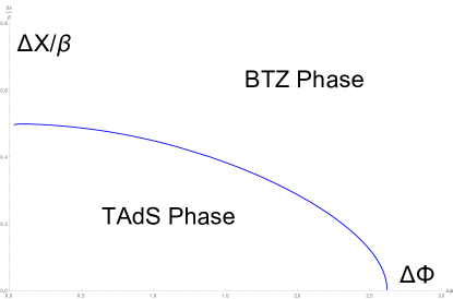
The connected EOW brane in thermal AdS3 is favored when , which leads to the condition , where this the temperature at the phase transition point, as a function of , is given by
| (6.49) |
Thus we can conclude that in the low temperature phase and high temperature phase , the connected EOW brane in thermal AdS3 and the disconnected EOW branes in BTZ are realized, respectively. This phase structure is depicted in Fig.27.
7 Transition matrix from AdS/BCFT and phase transition
In previous sections, we have introduced a brane-localized scalar field into the minimal AdS/BCFT construction [9, 10] and realized various novel configurations by designing the scalar. One of the most simple setup in this framework is realized by setting the potential to zero, i.e. considering a massless free scalar. In this case, the nontriviality can be introduced by considering a brane which has two asymptotic infinities and impose different boundary values of on each. Such setups are discussed in section 3.3 and section 6.
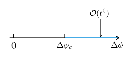
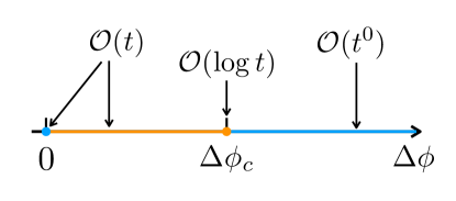
In this section, we construct a setup in this framework and argue that there exists a novel phase transition in its time evolution behavior induced by the parameter . More precisely, we consider a 1D quantum many-body system and a class of time-dependent transition matrices which is characterized by a single parameter. After seeing how this single parameter can be related to in an AdS3 gravity via the AdS/BCFT correspondence, we will argue that the time growth of the pseudo entropy [119, 132, 133] in this setup is when is sufficiently small, when is sufficiently large, and at the phase transition point. This behavior is similar to the measurement-induced phase transition of the entanglement entropy in 1D quantum many-body systems [120, 121, 122] when changing the measurement rate.
In the following, we will first explain the basic concepts of transition matrices and pseudo entropy. Then we will introduce our setup in the BCFT language and explain how it can be related to setups studied in section 3.3 and section 6 via the AdS/BCFT correspondence. After that, we will explain the details of the phase transition mentioned above and why we expect it exists.
7.1 Pseudo Entropy and The Setup
Pseudo entropy is a generalization of entanglement entropy, and it was firstly introduced in [119]. Let us consider a bipartite system composited by and . The total Hilbert space is given by
| (7.1) |
For two pure states which are not orthogonal to each other, the transition matrix is defined as
| (7.2) |
Such a transition matrix describes a post-selection or weak measurement [134, 135] procedure where one prepares an initial state , performs operations on it, and then post-selects it to . For example, the weak value [134, 135] of an operator can be obtained by computing .
The reduced transition matrix on is defined as
| (7.3) |
Note that the (reduced) transition matrix reduces to a standard (reduced) density matrix when . The pseudo entropy is defined by formally computing the von Neumann entropy
| (7.4) |
Note that the pseudo entropy is not an entropy in the sense that it does not satisfy all the axioms of entropy such as reality or convexity. However, it reduces to entanglement entropy when and hence is a generalization of it. Moreover, in holographic setups, the leading order of the pseudo entropy can be computed using the same recipe for holographic entanglement entropy [119].
While the entanglement entropy of a pure state counts the number of EPR pairs one can distill by performing local operations and classical communications (LOCC) on the state, the operational meaning of pseudo entropy for general transition matrices is unclear. For a special class of transition matrices, the pseudo entropy can be interpreted as the number of EPR pairs one can distill in the post-selection procedure described by [119]. However, despite the fact that its physical meaning is not completely clear, it has been found that pseudo entropy is useful for studying various physical systems such as phase transitions in quantum many-body systems [132, 133].
In the following, let us consider a 1D system defined on an infinite line. Starting from an area law state and time evolving it with a gapless Hamiltonian , the entanglement will grow linearly and the state will become a volume law state. More precisely, the entanglement entropy of a single interval with length in the time-evolved state will grow as and saturate to . This is well-known as the global quench setup [136, 137].
In CFT, such an initial state can be realized by a regularized boundary state [136, 137]
| (7.5) |
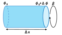
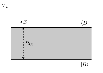
In the path integral language, one can consider a Euclidean strip parameterized by , where is the Euclidean time and is the spatial coordinate. Here, the boundary conditions imposed on and are the same. In this case, when focusing on the time slice , the state realized by the path integral over and that over are and respectively. By performing the analytic continuation , one can realize the time evolved state . It is well-known that the effective temperature of such a state is given by .
Let us consider a generalization of the setup described above. Instead of imposing the same boundary condition on the two boundaries, let us impose different ones. Denoting the boundary conditions imposed on and as and , respectively, the current path integral describes the following transition matrix
| (7.6) |
after performing the analytical continuation . In the following, let us divide the subsystem given by and consider the pseudo entropy associated with it.

7.2 Holographic Duals and Phase Transition
The setups with brane-localized free massless scalar naturally realize a class of the transition matrices (7.6) in the AdS/BCFT correspondence. The boundary values of the brane-localized scalar field on the two asymptotic infinities correspond to the boundary states imposed on the two boundaries on the BCFT side. In this sense, the boundary value of parameterizes the boundary states. Accordingly, we can write
| (7.7) |
where
| (7.8) |
The gravity dual of the Euclidean setup can been straightforward obtained from the results in section 6. In section 6, we have discussed the gravity dual of a BCFT defined on a manifold with topology , where we regard as the Euclidean time direction parameterized by and as the spatial direction parameterized by . Now we are considering a BCFT defined on , where we regard as the Euclidean time direction parameterized by and as the spatial direction parameterized by . While not precise, it is useful to consider the infinite system as the infinite radius limit of an . In this sense, the definitions of and used here are opposite to that used in section 6.
The , and in section 6 correspond to , and in the current section, respectively. Looking at the part of figure 27, one can see that there is a phase transition when changing and the phase transition point is given by . Since the coordinates of space and time are different between section 6 and this section, let us call the BTZ phase (thermal AdS phase) in section 6 the large phase (small phase) in this section to avoid confusion. Let us consider the Lorentzian counterparts for all these cases.
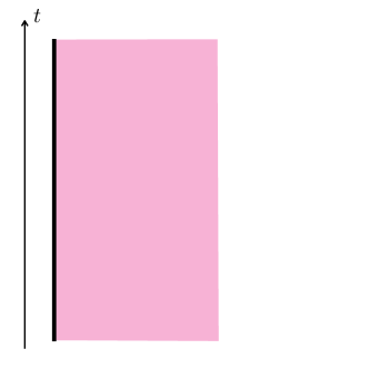
7.2.1 Small Phase
The small phase corresponds to the thermal AdS phase in section 6. The Euclidean gravity dual is given by a BTZ metric333Again, note that the time and space are opposite in section 6 and this setion.
| (7.9) |
with an end-of-the-world brane connecting the boundaries at the Euclidean past and future. Here, is determined by solving
| (7.10) |
where the functions and are given by figure 21. The effective temperature of the BTZ metric is given by
| (7.11) |
Accordingly, the corresponding Lorentzian setup is a one-sided BTZ black hole with temperature and an end-of-the-world brane falling behind the horizon. See figure 29 for a sketch. A crucial feature of the current setup is that, while the Euclidean path integral is not time reflection symmetric on the BCFT side, the geometry of the gravity dual is. All the non-reflection symmetric elements in the gravity dual is the scalar field . This feature allows us to get a real geometry corresponding to the Lorentzian setup by simply perform the analytical continuation. This is also true in other phases.

The pseudo entropy can be computed from the HRT surface extending from and ends on the brane. To grasp an intuition, let us firstly consider the case. This is nothing but the standard global quench setup [136, 137] or the Hartman-Maldacena setup [118]. In this case, the computation can be analytically performed [118] and the pseudo entropy reduces to the standard entanglement entropy after a global quench and turns out to be [118]
| (7.12) |
at late time. The linear behavior reflects the fact that the end-of-the-world brane goes deeper behind the horizon as the time evolves, and the coefficient reflects the temperature of the background geometry.
Although we are not going to explicitly compute the time evolution of the pseudo entropy for more general , it is natural to expect the late time behaviors of the brane dynamics are similar for different . Therefore, we conjecture that the leading order at late time is also
| (7.13) |
even in this case. We leave testing this conjecture as a future problem. See figure for a sketch of what we have found in the small phase.
7.2.2 Large Phase
The large phase corresponds to the BTZ phase in section 6. The Euclidean gravity dual is given by a thermal AdS
| (7.14) |
with two end-of-the-world branes extending from the two boundaries at the Euclidean past and future. Here, is determined by solving
| (7.15) |
where the functions and are given by figure 24. The effective temperature of the thermal AdS metric is given by
| (7.16) |
It is straightforward to find that the corresponding Lorentzian setup is a static thermal AdS with temperature and no time evolution. Moreover, there is no end-of-the-world branes involved in the Lorentzian configuration. See figure 31 for a sketch.
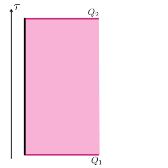
Accordingly, the holographic pseudo entropy has no time evolution either, i.e.
| (7.17) |
See figure 32 for a sketch of what we have found in the large phase.
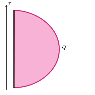
7.2.3 The Phase Transition Point
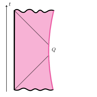
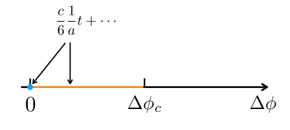
As the last case, let us consider the phase transition point . The corresponding Euclidean setup has been already studied in section 3.3. By performing the analytic continuation, one can find that the Lorentzian setup is a Poincare AdS with an end-of-the-world brane accelerating and falling towards the Poincare horizon. See figure 33 for a sketch.
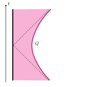
If we approximates the holographic pseudo entropy with the minimal geodesic lying in the time slice , one can find the time growth of the approximated pseudo entropy is
| (7.18) |
In general, when there is an end-of-the-world brane approaching the speed of light and falling towards the Poincaré horizon, the coefficient can be modified by the back reaction444The HRT surface goes outside of the Poincaé patch when the end-of-the-world brane approaches the speed of light and falls towards the Poincaré horizon. The segment outside of the Poincaé patch can modify the coefficient of the term in the time evolution. See [63, 64] for details. of the end-of-the-world brane but the logarithmic behavior is robust.
| (7.19) |
It would be an interesting future direction to determine the coefficient in this case. See figure 34 for a sketch of what we have found in this phase transition.
7.3 Possible connection to measurement-induced phase transition
For our transition matrix in a holographic two dimensional CFT, we observed the time evolution of pseudo entropy changes from the linear growth (small phase with BTZ geometry) to the trivial one (large phase with thermal AdS geometry) when turning up the parameter , and the behavior at the phase transition point with Poincaré geometry is . This looks very similar to the behavior of entanglement entropy under the measurement-induced phase transition in 1D quantum many-body systems [120, 121, 122]. Motivated by this, we would like to propose below a possible interpretation of our phase transition of transition matrix as a version of the measurement-induced phase transition.
To begin with, let us first point out that the gravity side of the current setup effectively realize a classical open system. In the current setup, the BCFT side is a path integral which represents a transition matrix, which means that the BCFT side is not in a standard quantum state, but a combination of two quantum states. On the other hand, the gravity side in the Lorentzian signature can be determined by solving the Einstein equation with the initial condition at and turns out to be a standard state in classical gravity. The only exotic part on the gravity side is that the brane-localized scalar field takes imaginary values and turns out to be a ghost in the Lorentzian signature. This can be easily seen from the equation of motion of the scalar field (3.29) with the Wick rotation performed. As a result, the energy in the gravity sector leaks to the brane-localized scalar sector under the time evolution, and the current setup effectively realize an open system when viewing from the bulk gravity sector. The “openness” of the system is characterized by the shift of the scalar field .
The behavior on the gravity side discussed above motivates us to conjecture that the field theory side effectively realize a single quantum state under a non-unitary time evolution which describes a quantum open system555Note that the canonical explanation on the field theory side is a combination of two quantum states under unitary time evolution.. In this explanation, the quantity computed by the HRT formula turns out to be the entanglement entropy of the single quantum state under a non-unitary time evolution, but not the pseudo entropy of the transition matrix under a unitary time evolution. Again, the “openness” of the quantum system is characterized by the shift of the scalar field . When gets larger, the system gets more open to the outside environment which may be interpreted as measurements, and the entanglement growth gets reduced and experiences the phase transition. Indeed, this is very similar to the measurement-induced phase transition.
To summary, discussions above suggest that our time-dependent solution with the EOW brane with a ghost field may be a gravity dual of an open quantum system where a quantum system evolves in a non-unitary way, driven by e.g. non-hermitian Hamiltonians or projection measurements. Note that if we perform projection measurements in the UV degrees of freedom, then the EOW brane should intersect with the AdS boundary as in the setups studied earlier [59, 72]. Instead in our present construction, we expect non-unitary operations such as projections are acted on the IR degrees of freedom as the EOW brane is inserted in the interior. Such non-unitary EOW branes seem to imply a new holographic relation including open systems. We leave more detailed studies of this interpretation for an important future problem.
8 Conclusions and Discussions
In this paper, we studied the dynamics of a scalar field localized on the end-of-the-world (EOW) brane as a new extension of the minimal setup of AdS/BCFT. This brane-localized scalar field is dual to a boundary primary operator. As opposed to setups with bulk scalar fields, it is often possible to analytically solve the equation of motion at least partially. Owing to this advantage, we obtained various new solutions which are only possible in the presence of the scalar field.
Firstly, we found planar solutions which are gravity duals of boundary RG flows. Next, by imposing rotational invariance, we obtained hemisphere, annulus and cone shaped solutions in the Poincaré AdS3. Among them, annulus and cone shaped ones are impossible in the minimal AdS/BCFT model. We also give interpretations from the viewpoint of boundary RG flows for the hemisphere and annulus shaped solutions. We leave the field theoretic interpretation of the cone shaped solutions as a future problem. At the intuitive level, they look like poking small holes in the space. Notice that these constructions of above solutions can be done in any dimension in a similar way, though we often presented solutions in AdSBCFT2 explicitly.
We can also get intriguing solutions for BCFTs on strips. Even when the two boundaries of the strip have different values of the scalar potential, we can construct a connected EOW brane in our setup. We find that there is a phase transition point in the value of the difference of the scalar potential . If is smaller than the value at the phase transition point, the gravity dual is given by a connected EOW brane in thermal AdS3. If it is larger, then the dual geometry is given by disconnected EOW branes in BTZ. At the phase transition point and at the zero temperature, the dual is a connected EOW brane in the Poincaré AdS3. Our phase diagram Fig.27 is analogous to the Hawking-Page transition with a chemical potential, which describes the physics of confinement/deconfinement phase transition.
We can also regard these solutions as transition matrices via a Wick rotation. In this interpretation, the phase transition we found describes the transition of dynamical evolutions of pseudo entropy from the area law to volume law . At the phase transition point we may expect the logarithmic evolution in two dimensions. It is intriguing to note that in the corresponding Lorentzian gravity dual, the EOW brane does not intersect with the AdS boundary, which can be regarded as a deformation of [118]. We may try to interpret this time-dependent geometry as a gravity dual of the time evolution of a certain quantum state in the CFT. However, the new thing in our solution is that the scalar field on the EOW brane takes imaginary values, which is equivalent to a ghost-like scalar on the brane. The amount of such non-unitarity is controlled by the parameter . The above results imply that as the non-unitary effect gets larger, the entanglement growth gets reduced. This is analogous to the measurement-induced phase transition [120, 121, 122]. This suggests that our time-dependent solution with the EOW brane with a ghost field may be a gravity dual of an open quantum system where a quantum system evolves in a non-unitary way derived by e.g. non-hermitian Hamiltonians or projection measurements. This obviously deserves future investigations.
Since our setup is a small extension of the minimal AdS/BCFT, it would be interesting to analyze setups of AdS/BCFT with richer contents of brane-localized fields such as multiple scalar fields and gauge fields. Such further extensions may allow us to study boundary problems in condensed matter physics. Another application may be to build new holographic cosmology models, by taking into account the brane-world dynamics of localized graviton on EOW branes. Finally, since we relied on a bottom-up construction in this paper, it will be important to consider the string theory realizations of our models.
Acknowledgements
We are grateful to Brian Swingle and Tomonori Ugajin for useful discussions. This work is supported by the Simons Foundation through the “It from Qubit” collaboration and by MEXT KAKENHI Grant-in-Aid for Transformative Research Areas (A) through the “Extreme Universe” collaboration: Grant Number 21H05187. This work is also supported by Inamori Research Institute for Science and by JSPS Grant-in-Aid for Scientific Research (A) No. 21H04469. ZW is supported by Grant-in-Aid for JSPS Fellows No. 20J23116. TT would like to thank 2022 Simons Collaboration on It from Qubit Annual Meeting where a part of the present work was done.
Appendix A The round-shaped solution of
We solve in (4):
| (A.1) |
under some boundary conditions. In the considering region, we can simplify into
| (A.2) |
since . Introducing , we have
| (A.3) |
First, we can easily find soltions for the case of equal sign
| (A.4) |
As mentioned in Chapter 4.1, this solution corresponds to a part of an exact sphere. Now we make dependent of . Then inequality (A.3) can be read as
| (A.5) |
equivalently, .
Next, We restrict by boundary conditions. In the Type I, for example, we impose and on the general solution
| (A.6) |
and, therefore, solutions must satisfy and . The same applies to the Type III. On the other hand, in the Type II, we impose and . This means
| (A.7) |
Therefore, we can conclude must be displayed by
| (A.8) |
where function satisfies and is finite.
References
- [1] J. L. Cardy, Conformal Invariance and Surface Critical Behavior, Nucl. Phys. B 240 (1984) 514–532.
- [2] J. L. Cardy, Boundary conformal field theory, hep-th/0411189.
- [3] D. M. McAvity and H. Osborn, Energy momentum tensor in conformal field theories near a boundary, Nucl. Phys. B 406 (1993) 655–680, [hep-th/9302068].
- [4] D. M. McAvity and H. Osborn, Conformal field theories near a boundary in general dimensions, Nucl. Phys. B 455 (1995) 522–576, [cond-mat/9505127].
- [5] J. M. Maldacena, The Large N limit of superconformal field theories and supergravity, Adv. Theor. Math. Phys. 2 (1998) 231–252, [hep-th/9711200].
- [6] S. S. Gubser, I. R. Klebanov, and A. M. Polyakov, Gauge theory correlators from noncritical string theory, Phys. Lett. B 428 (1998) 105–114, [hep-th/9802109].
- [7] E. Witten, Anti-de Sitter space and holography, Adv. Theor. Math. Phys. 2 (1998) 253–291, [hep-th/9802150].
- [8] A. Karch and L. Randall, Open and closed string interpretation of SUSY CFT’s on branes with boundaries, JHEP 06 (2001) 063, [hep-th/0105132].
- [9] T. Takayanagi, Holographic Dual of BCFT, Phys. Rev. Lett. 107 (2011) 101602, [arXiv:1105.5165].
- [10] M. Fujita, T. Takayanagi, and E. Tonni, Aspects of AdS/BCFT, JHEP 11 (2011) 043, [arXiv:1108.5152].
- [11] M. Nozaki, T. Takayanagi, and T. Ugajin, Central Charges for BCFTs and Holography, JHEP 06 (2012) 066, [arXiv:1205.1573].
- [12] S. Ryu and T. Takayanagi, Holographic derivation of entanglement entropy from AdS/CFT, Phys. Rev. Lett. 96 (2006) 181602, [hep-th/0603001].
- [13] S. Ryu and T. Takayanagi, Aspects of Holographic Entanglement Entropy, JHEP 08 (2006) 045, [hep-th/0605073].
- [14] V. E. Hubeny, M. Rangamani, and T. Takayanagi, A Covariant holographic entanglement entropy proposal, JHEP 07 (2007) 062, [arXiv:0705.0016].
- [15] R.-X. Miao, C.-S. Chu, and W.-Z. Guo, New proposal for a holographic boundary conformal field theory, Phys. Rev. D 96 (2017), no. 4 046005, [arXiv:1701.04275].
- [16] A. Almheiri, R. Mahajan, J. Maldacena, and Y. Zhao, The Page curve of Hawking radiation from semiclassical geometry, JHEP 03 (2020) 149, [arXiv:1908.10996].
- [17] G. Penington, Entanglement Wedge Reconstruction and the Information Paradox, JHEP 09 (2020) 002, [arXiv:1905.08255].
- [18] A. Almheiri, N. Engelhardt, D. Marolf, and H. Maxfield, The entropy of bulk quantum fields and the entanglement wedge of an evaporating black hole, JHEP 12 (2019) 063, [arXiv:1905.08762].
- [19] L. Randall and R. Sundrum, A Large mass hierarchy from a small extra dimension, Phys. Rev. Lett. 83 (1999) 3370–3373, [hep-ph/9905221].
- [20] L. Randall and R. Sundrum, An Alternative to compactification, Phys. Rev. Lett. 83 (1999) 4690–4693, [hep-th/9906064].
- [21] S. S. Gubser, AdS / CFT and gravity, Phys. Rev. D 63 (2001) 084017, [hep-th/9912001].
- [22] A. Karch and L. Randall, Locally localized gravity, JHEP 05 (2001) 008, [hep-th/0011156].
- [23] S. B. Giddings, E. Katz, and L. Randall, Linearized gravity in brane backgrounds, JHEP 03 (2000) 023, [hep-th/0002091].
- [24] T. Shiromizu and D. Ida, Anti-de Sitter no hair, AdS / CFT and the brane world, Phys. Rev. D 64 (2001) 044015, [hep-th/0102035].
- [25] T. Shiromizu, T. Torii, and D. Ida, Brane world and holography, JHEP 03 (2002) 007, [hep-th/0105256].
- [26] S. Nojiri, S. D. Odintsov, and S. Zerbini, Quantum (in)stability of dilatonic AdS backgrounds and holographic renormalization group with gravity, Phys. Rev. D 62 (2000) 064006, [hep-th/0001192].
- [27] S. Nojiri and S. D. Odintsov, Brane world inflation induced by quantum effects, Phys. Lett. B 484 (2000) 119–123, [hep-th/0004097].
- [28] S. W. Hawking, T. Hertog, and H. S. Reall, Brane new world, Phys. Rev. D 62 (2000) 043501, [hep-th/0003052].
- [29] K. Koyama and J. Soda, Strongly coupled CFT in FRW universe from AdS / CFT correspondence, JHEP 05 (2001) 027, [hep-th/0101164].
- [30] S. Kanno and J. Soda, Brane world effective action at low-energies and AdS / CFT, Phys. Rev. D 66 (2002) 043526, [hep-th/0205188].
- [31] R. Emparan, R. Luna, R. Suzuki, M. Tomašević, and B. Way, Holographic duals of evaporating black holes, arXiv:2301.02587.
- [32] A. Almheiri, R. Mahajan, and J. E. Santos, Entanglement islands in higher dimensions, SciPost Phys. 9 (2020), no. 1 001, [arXiv:1911.09666].
- [33] M. Rozali, J. Sully, M. Van Raamsdonk, C. Waddell, and D. Wakeham, Information radiation in BCFT models of black holes, JHEP 05 (2020) 004, [arXiv:1910.12836].
- [34] H. Z. Chen, Z. Fisher, J. Hernandez, R. C. Myers, and S.-M. Ruan, Information Flow in Black Hole Evaporation, JHEP 03 (2020) 152, [arXiv:1911.03402].
- [35] V. Balasubramanian, A. Kar, O. Parrikar, G. Sárosi, and T. Ugajin, Geometric secret sharing in a model of Hawking radiation, JHEP 01 (2021) 177, [arXiv:2003.05448].
- [36] H. Geng and A. Karch, Massive islands, JHEP 09 (2020) 121, [arXiv:2006.02438].
- [37] H. Z. Chen, R. C. Myers, D. Neuenfeld, I. A. Reyes, and J. Sandor, Quantum Extremal Islands Made Easy, Part I: Entanglement on the Brane, JHEP 10 (2020) 166, [arXiv:2006.04851].
- [38] H. Z. Chen, R. C. Myers, D. Neuenfeld, I. A. Reyes, and J. Sandor, Quantum Extremal Islands Made Easy, Part II: Black Holes on the Brane, JHEP 12 (2020) 025, [arXiv:2010.00018].
- [39] R. Bousso and E. Wildenhain, Gravity/ensemble duality, Phys. Rev. D 102 (2020), no. 6 066005, [arXiv:2006.16289].
- [40] H. Z. Chen, Z. Fisher, J. Hernandez, R. C. Myers, and S.-M. Ruan, Evaporating Black Holes Coupled to a Thermal Bath, JHEP 01 (2021) 065, [arXiv:2007.11658].
- [41] Y. Chen, V. Gorbenko, and J. Maldacena, Bra-ket wormholes in gravitationally prepared states, JHEP 02 (2021) 009, [arXiv:2007.16091].
- [42] I. Akal, Y. Kusuki, N. Shiba, T. Takayanagi, and Z. Wei, Entanglement Entropy in a Holographic Moving Mirror and the Page Curve, Phys. Rev. Lett. 126 (2021), no. 6 061604, [arXiv:2011.12005].
- [43] M. Miyaji, Island for gravitationally prepared state and pseudo entanglement wedge, JHEP 12 (2021) 013, [arXiv:2109.03830].
- [44] I. Akal, Y. Kusuki, N. Shiba, T. Takayanagi, and Z. Wei, Holographic moving mirrors, Class. Quant. Grav. 38 (2021), no. 22 224001, [arXiv:2106.11179].
- [45] H. Geng, A. Karch, C. Perez-Pardavila, S. Raju, L. Randall, M. Riojas, and S. Shashi, Entanglement phase structure of a holographic BCFT in a black hole background, JHEP 05 (2022) 153, [arXiv:2112.09132].
- [46] A. Bhattacharya, A. Bhattacharyya, P. Nandy, and A. K. Patra, Bath deformations, islands, and holographic complexity, Phys. Rev. D 105 (2022), no. 6 066019, [arXiv:2112.06967].
- [47] Q.-L. Hu, D. Li, R.-X. Miao, and Y.-Q. Zeng, AdS/BCFT and Island for curvature-squared gravity, JHEP 09 (2022) 037, [arXiv:2202.03304].
- [48] T. Anous, M. Meineri, P. Pelliconi, and J. Sonner, Sailing past the End of the World and discovering the Island, SciPost Phys. 13 (2022), no. 3 075, [arXiv:2202.11718].
- [49] T. Kawamoto, T. Mori, Y.-k. Suzuki, T. Takayanagi, and T. Ugajin, Holographic local operator quenches in BCFTs, JHEP 05 (2022) 060, [arXiv:2203.03851].
- [50] L. Bianchi, S. De Angelis, and M. Meineri, Radiation, entanglement and islands from a boundary local quench, arXiv:2203.10103.
- [51] I. Akal, T. Kawamoto, S.-M. Ruan, T. Takayanagi, and Z. Wei, Page curve under final state projection, Phys. Rev. D 105 (2022), no. 12 126026, [arXiv:2112.08433].
- [52] I. Akal, T. Kawamoto, S.-M. Ruan, T. Takayanagi, and Z. Wei, Zoo of holographic moving mirrors, JHEP 08 (2022) 296, [arXiv:2205.02663].
- [53] H. Geng, L. Randall, and E. Swanson, BCFT in a black hole background: an analytical holographic model, JHEP 12 (2022) 056, [arXiv:2209.02074].
- [54] A. Bhattacharjee and M. Saha, JT gravity from holographic reduction of 3D asymptotically flat spacetime, JHEP 01 (2023) 138, [arXiv:2211.13415].
- [55] M. Fujita, M. Kaminski, and A. Karch, SL(2,Z) Action on AdS/BCFT and Hall Conductivities, JHEP 07 (2012) 150, [arXiv:1204.0012].
- [56] T. Ugajin, Two dimensional quantum quenches and holography, arXiv:1311.2562.
- [57] J. Erdmenger, M. Flory, and M.-N. Newrzella, Bending branes for DCFT in two dimensions, JHEP 01 (2015) 058, [arXiv:1410.7811].
- [58] J. Erdmenger, M. Flory, C. Hoyos, M.-N. Newrzella, A. O’Bannon, and J. Wu, Holographic impurities and Kondo effect, Fortsch. Phys. 64 (2016) 322–329, [arXiv:1511.09362].
- [59] T. Numasawa, N. Shiba, T. Takayanagi, and K. Watanabe, EPR Pairs, Local Projections and Quantum Teleportation in Holography, JHEP 08 (2016) 077, [arXiv:1604.01772].
- [60] D. Seminara, J. Sisti, and E. Tonni, Corner contributions to holographic entanglement entropy in AdS4/BCFT3, JHEP 11 (2017) 076, [arXiv:1708.05080].
- [61] D. Seminara, J. Sisti, and E. Tonni, Holographic entanglement entropy in AdS4/BCFT3 and the Willmore functional, JHEP 08 (2018) 164, [arXiv:1805.11551].
- [62] Y. Hikida, Y. Kusuki, and T. Takayanagi, Eigenstate thermalization hypothesis and modular invariance of two-dimensional conformal field theories, Phys. Rev. D 98 (2018), no. 2 026003, [arXiv:1804.09658].
- [63] T. Shimaji, T. Takayanagi, and Z. Wei, Holographic Quantum Circuits from Splitting/Joining Local Quenches, JHEP 03 (2019) 165, [arXiv:1812.01176].
- [64] P. Caputa, T. Numasawa, T. Shimaji, T. Takayanagi, and Z. Wei, Double Local Quenches in 2D CFTs and Gravitational Force, JHEP 09 (2019) 018, [arXiv:1905.08265].
- [65] M. Mezei and J. Virrueta, Exploring the Membrane Theory of Entanglement Dynamics, JHEP 02 (2020) 013, [arXiv:1912.11024].
- [66] W. Reeves, M. Rozali, P. Simidzija, J. Sully, C. Waddell, and D. Wakeham, Looking for (and not finding) a bulk brane, JHEP 12 (2021) 002, [arXiv:2108.10345].
- [67] Y. Kusuki, Analytic bootstrap in 2D boundary conformal field theory: towards braneworld holography, JHEP 03 (2022) 161, [arXiv:2112.10984].
- [68] M. Miyaji, T. Takayanagi, and T. Ugajin, Spectrum of End of the World Branes in Holographic BCFTs, JHEP 06 (2021) 023, [arXiv:2103.06893].
- [69] T. Numasawa and I. Tsiares, Universal dynamics of heavy operators in boundary CFT2, JHEP 08 (2022) 156, [arXiv:2202.01633].
- [70] J. Chandra and T. Hartman, Coarse graining pure states in AdS/CFT, arXiv:2206.03414.
- [71] Y. Kusuki, Semiclassical gravity from averaged boundaries in two-dimensional boundary conformal field theories, Phys. Rev. D 106 (2022), no. 6 066020, [arXiv:2206.03035].
- [72] S. Antonini, G. Bentsen, C. Cao, J. Harper, S.-K. Jian, and B. Swingle, Holographic measurement and bulk teleportation, JHEP 12 (2022) 124, [arXiv:2209.12903].
- [73] Y. Kusuki and Z. Wei, AdS/BCFT from conformal bootstrap: construction of gravity with branes and particles, JHEP 01 (2023) 108, [arXiv:2210.03107].
- [74] M. Gutperle and J. Samani, Holographic RG-flows and Boundary CFTs, Phys. Rev. D 86 (2012) 106007, [arXiv:1207.7325].
- [75] J. Estes, K. Jensen, A. O’Bannon, E. Tsatis, and T. Wrase, On Holographic Defect Entropy, JHEP 05 (2014) 084, [arXiv:1403.6475].
- [76] N. Kobayashi, T. Nishioka, Y. Sato, and K. Watanabe, Towards a -theorem in defect CFT, JHEP 01 (2019) 039, [arXiv:1810.06995].
- [77] Y. Sato, Boundary entropy under ambient RG flow in the AdS/BCFT model, Phys. Rev. D 101 (2020), no. 12 126004, [arXiv:2004.04929].
- [78] S. Chapman, D. Ge, and G. Policastro, Holographic Complexity for Defects Distinguishes Action from Volume, JHEP 05 (2019) 049, [arXiv:1811.12549].
- [79] Y. Sato and K. Watanabe, Does Boundary Distinguish Complexities?, JHEP 11 (2019) 132, [arXiv:1908.11094].
- [80] P. Braccia, A. L. Cotrone, and E. Tonni, Complexity in the presence of a boundary, JHEP 02 (2020) 051, [arXiv:1910.03489].
- [81] Y. Sato, Complexity in a moving mirror model, Phys. Rev. D 105 (2022), no. 8 086016, [arXiv:2108.04637].
- [82] J. Hernandez, R. C. Myers, and S.-M. Ruan, Quantum extremal islands made easy. Part III. Complexity on the brane, JHEP 02 (2021) 173, [arXiv:2010.16398].
- [83] S. Collier, D. Mazac, and Y. Wang, Bootstrapping Boundaries and Branes, arXiv:2112.00750.
- [84] A. Chalabi, C. P. Herzog, A. O’Bannon, B. Robinson, and J. Sisti, Weyl anomalies of four dimensional conformal boundaries and defects, JHEP 02 (2022) 166, [arXiv:2111.14713].
- [85] A. Belin, S. Biswas, and J. Sully, The spectrum of boundary states in symmetric orbifolds, JHEP 01 (2022) 123, [arXiv:2110.05491].
- [86] K. Suzuki, Y.-k. Suzuki, T. Tsuda, and M. Watanabe, Information metric on the boundary, arXiv:2212.10899.
- [87] S. Cooper, M. Rozali, B. Swingle, M. Van Raamsdonk, C. Waddell, and D. Wakeham, Black hole microstate cosmology, JHEP 07 (2019) 065, [arXiv:1810.10601].
- [88] S. Antonini and B. Swingle, Cosmology at the end of the world, Nature Phys. 16 (2020), no. 8 881–886, [arXiv:1907.06667].
- [89] M. Van Raamsdonk, Comments on wormholes, ensembles, and cosmology, JHEP 12 (2021) 156, [arXiv:2008.02259].
- [90] M. Van Raamsdonk, Cosmology from confinement?, JHEP 03 (2022) 039, [arXiv:2102.05057].
- [91] C. Waddell, Bottom-up holographic models for cosmology, JHEP 09 (2022) 176, [arXiv:2203.03096].
- [92] Y.-k. Suzuki, One-loop correction to the AdS/BCFT partition function in three-dimensional pure gravity, Phys. Rev. D 105 (2022), no. 2 026023, [arXiv:2106.00206].
- [93] H. Omiya and Z. Wei, Causal structures and nonlocality in double holography, JHEP 07 (2022) 128, [arXiv:2107.01219].
- [94] K. Suzuki and T. Takayanagi, BCFT and Islands in two dimensions, JHEP 06 (2022) 095, [arXiv:2202.08462].
- [95] Y.-k. Suzuki and S. Terashima, On the dynamics in the AdS/BCFT correspondence, JHEP 09 (2022) 103, [arXiv:2205.10600].
- [96] K. Izumi, T. Shiromizu, K. Suzuki, T. Takayanagi, and N. Tanahashi, Brane dynamics of holographic BCFTs, JHEP 10 (2022) 050, [arXiv:2205.15500].
- [97] M. Chiodaroli, E. D’Hoker, Y. Guo, and M. Gutperle, Exact half-BPS string-junction solutions in six-dimensional supergravity, JHEP 12 (2011) 086, [arXiv:1107.1722].
- [98] M. Chiodaroli, E. D’Hoker, and M. Gutperle, Holographic duals of Boundary CFTs, JHEP 07 (2012) 177, [arXiv:1205.5303].
- [99] A. Karch and L. Randall, Geometries with mismatched branes, JHEP 09 (2020) 166, [arXiv:2006.10061].
- [100] C. Bachas, S. Chapman, D. Ge, and G. Policastro, Energy Reflection and Transmission at 2D Holographic Interfaces, Phys. Rev. Lett. 125 (2020), no. 23 231602, [arXiv:2006.11333].
- [101] P. Simidzija and M. Van Raamsdonk, Holo-ween, JHEP 12 (2020) 028, [arXiv:2006.13943].
- [102] H. Ooguri and T. Takayanagi, Cobordism Conjecture in AdS, arXiv:2006.13953.
- [103] M. V. Raamsdonk and C. Waddell, Holographic and localization calculations of boundary F for = 4 SUSY Yang-Mills theory, JHEP 02 (2021) 222, [arXiv:2010.14520].
- [104] C. F. Uhlemann, Islands and Page curves in 4d from Type IIB, JHEP 08 (2021) 104, [arXiv:2105.00008].
- [105] L. Coccia and C. F. Uhlemann, Mapping out the internal space in AdS/BCFT with Wilson loops, JHEP 03 (2022) 127, [arXiv:2112.14648].
- [106] A. Karch, H. Sun, and C. F. Uhlemann, Double holography in string theory, JHEP 10 (2022) 012, [arXiv:2206.11292].
- [107] I. Akal, Y. Kusuki, T. Takayanagi, and Z. Wei, Codimension two holography for wedges, Phys. Rev. D 102 (2020), no. 12 126007, [arXiv:2007.06800].
- [108] R.-X. Miao, An Exact Construction of Codimension two Holography, JHEP 01 (2021) 150, [arXiv:2009.06263].
- [109] H. Geng, A. Karch, C. Perez-Pardavila, S. Raju, L. Randall, M. Riojas, and S. Shashi, Jackiw-Teitelboim Gravity from the Karch-Randall Braneworld, Phys. Rev. Lett. 129 (2022), no. 23 231601, [arXiv:2206.04695].
- [110] H. Geng, Aspects of AdS2 quantum gravity and the Karch-Randall braneworld, JHEP 09 (2022) 024, [arXiv:2206.11277].
- [111] N. Ogawa, T. Takayanagi, T. Tsuda, and T. Waki, Wedge holography in flat space and celestial holography, Phys. Rev. D 107 (2023), no. 2 026001, [arXiv:2207.06735].
- [112] J. H. Lee, D. Neuenfeld, and A. Shukla, Bounds on gravitational brane couplings and tomography in AdS3 black hole microstates, JHEP 10 (2022) 139, [arXiv:2206.06511].
- [113] J. Erdmenger, C. Hoyos, A. O’Bannon, and J. Wu, A Holographic Model of the Kondo Effect, JHEP 12 (2013) 086, [arXiv:1310.3271].
- [114] J. Erdmenger, M. Flory, C. Hoyos, M.-N. Newrzella, and J. M. S. Wu, Entanglement Entropy in a Holographic Kondo Model, Fortsch. Phys. 64 (2016) 109–130, [arXiv:1511.03666].
- [115] J. Erdmenger, C. M. Melby-Thompson, and C. Northe, Holographic RG Flows for Kondo-like Impurities, JHEP 05 (2020) 075, [arXiv:2001.04991].
- [116] M. Miyaji and C. Murdia, Holographic BCFT with a Defect on the End-of-the-World brane, JHEP 11 (2022) 123, [arXiv:2208.13783].
- [117] S. Biswas, J. Kastikainen, S. Shashi, and J. Sully, Holographic BCFT spectra from brane mergers, JHEP 11 (2022) 158, [arXiv:2209.11227].
- [118] T. Hartman and J. Maldacena, Time Evolution of Entanglement Entropy from Black Hole Interiors, JHEP 05 (2013) 014, [arXiv:1303.1080].
- [119] Y. Nakata, T. Takayanagi, Y. Taki, K. Tamaoka, and Z. Wei, New holographic generalization of entanglement entropy, Phys. Rev. D 103 (2021), no. 2 026005, [arXiv:2005.13801].
- [120] B. Skinner, J. Ruhman, and A. Nahum, Measurement-Induced Phase Transitions in the Dynamics of Entanglement, Phys. Rev. X 9 (2019), no. 3 031009, [arXiv:1808.05953].
- [121] Y. Li, X. Chen, and M. P. A. Fisher, Quantum Zeno effect and the many-body entanglement transition, Phys. Rev. B 98 (2018), no. 20 205136, [arXiv:1808.06134].
- [122] Y. Li, X. Chen, and M. P. A. Fisher, Measurement-driven entanglement transition in hybrid quantum circuits, Phys. Rev. B 100 (2019), no. 13 134306, [arXiv:1901.08092].
- [123] J. D. Brown and M. Henneaux, Central Charges in the Canonical Realization of Asymptotic Symmetries: An Example from Three-Dimensional Gravity, Commun. Math. Phys. 104 (1986) 207–226.
- [124] P. Calabrese and J. L. Cardy, Entanglement entropy and quantum field theory, J. Stat. Mech. 0406 (2004) P06002, [hep-th/0405152].
- [125] I. Affleck and A. W. W. Ludwig, Universal noninteger ’ground state degeneracy’ in critical quantum systems, Phys. Rev. Lett. 67 (1991) 161–164.
- [126] D. Friedan and A. Konechny, On the boundary entropy of one-dimensional quantum systems at low temperature, Phys. Rev. Lett. 93 (2004) 030402, [hep-th/0312197].
- [127] I. R. Klebanov and E. Witten, AdS / CFT correspondence and symmetry breaking, Nucl. Phys. B 556 (1999) 89–114, [hep-th/9905104].
- [128] S. W. Hawking and D. N. Page, Thermodynamics of Black Holes in anti-De Sitter Space, Commun. Math. Phys. 87 (1983) 577.
- [129] E. Witten, Anti-de Sitter space, thermal phase transition, and confinement in gauge theories, Adv. Theor. Math. Phys. 2 (1998) 505–532, [hep-th/9803131].
- [130] M. Banados, Three-dimensional quantum geometry and black holes, AIP Conf. Proc. 484 (1999), no. 1 147–169, [hep-th/9901148].
- [131] M. M. Roberts, Time evolution of entanglement entropy from a pulse, JHEP 12 (2012) 027, [arXiv:1204.1982].
- [132] A. Mollabashi, N. Shiba, T. Takayanagi, K. Tamaoka, and Z. Wei, Pseudo Entropy in Free Quantum Field Theories, Phys. Rev. Lett. 126 (2021), no. 8 081601, [arXiv:2011.09648].
- [133] A. Mollabashi, N. Shiba, T. Takayanagi, K. Tamaoka, and Z. Wei, Aspects of pseudoentropy in field theories, Phys. Rev. Res. 3 (2021), no. 3 033254, [arXiv:2106.03118].
- [134] Y. Aharonov, D. Z. Albert, and L. Vaidman, How the result of a measurement of a component of the spin of a spin-1/2 particle can turn out to be 100, Phys. Rev. Lett. 60 (1988) 1351–1354.
- [135] J. Dressel, M. Malik, F. M. Miatto, A. N. Jordan, and R. W. Boyd, Colloquium: Understanding quantum weak values: Basics and applications, Rev. Mod. Phys. 86 (Mar, 2014) 307–316.
- [136] P. Calabrese and J. L. Cardy, Time-dependence of correlation functions following a quantum quench, Phys. Rev. Lett. 96 (2006) 136801, [cond-mat/0601225].
- [137] P. Calabrese and J. Cardy, Quantum quenches in 1 + 1 dimensional conformal field theories, J. Stat. Mech. 1606 (2016), no. 6 064003, [arXiv:1603.02889].