A nonlocal Lagrangian traffic flow model and the zero-filter limit

Abstract.

In this study, we start from a Follow-the-Leaders model for traffic flow that is based on a weighted harmonic mean (in Lagrangian coordinates) of the downstream car density. This results in a nonlocal Lagrangian partial differential equation (PDE) model for traffic flow. We demonstrate the well-posedness of the Lagrangian model in the $L^{1}$ sense. Additionally, we rigorously show that our model coincides with the Lagrangian formulation of the local LWR model in the “zero-filter” (nonlocal-to-local) limit. We present numerical simulations of the new model. One significant advantage of the proposed model is that it allows for simple proofs of (i) estimates that do not depend on the “filter size” and (ii) the dissipation of an arbitrary convex entropy.

1. Introduction

The LWR model, developed by Lighthill, Whitham, and Richards [23] more than six decades ago, was the first macroscopic traffic model. The basic form of the LWR model is a hyperbolic conservation law [13], which is a PDE that states that the total number of vehicles on a given stretch of road must remain constant over time. This is expressed mathematically as a continuity equation, which relates the flow of vehicles $uV$ into and out of a given region to the change in the density $u$ of vehicles within that region. The LWR model also includes equations that describe how the speed $V$ of vehicles changes over time $t$ and space $x$. These equations are based on the assumption that the speed $V$ of a vehicle located at a point $x$ at time $t$ is determined by the density $u$ of vehicles at $(t,x)$, $V=V(u(t,x))$, and that the speed of a vehicle will tend to decrease as the density of surrounding vehicles increases, $V^{\prime}(\cdot)\leq 0$. We refer to $uV(u)$ as the flux function and the conservation law

(1.1) $$\partial_{t}u+\partial_{x}\bigl{(}uV(u)\bigr{)}=0$$

as the original LWR model. There have been many generalisations of the LWR model over the years. For a comprehensive discussion of traffic flow data and the various models used to mathematically represent it, we recommend consulting the book [28].

The original LWR model is based on local PDEs, which means that the speed function $V$ is determined by the values of the car density at a single point $x$ in space. There have been numerous efforts to develop alternative speed functions. In particular, many authors examined nonlocal generalisations of the original LWR model, taking into account the look-ahead distance of drivers in order to better model their behavior. Some models assume that drivers react to the mean downstream traffic density, while others assume that they react to the mean downstream velocity. The corresponding nonlocal LWR models take the form

(1.2) $$\partial_{t}u+\partial_{x}\left(uV\left(\overline{u}\right)\right)=0,\quad\partial_{t}u+\partial_{x}\left(u\overline{V(u)}\right)=0,$$

where, for a given integrable function $v=v(x)$, $\overline{v}(x):=\int_{x}^{\infty}\Phi_{\alpha}(y-x)v(y)\,dy$. The anisotropic kernel $\Phi_{\alpha}$ characterizes the nonlocal effect through the “filter size” $\alpha>0$. It is a nonnegative, non-increasing, and $C^{1}$ function defined on the nonnegative real numbers, and it has unit mass: $\int_{0}^{\infty}\Phi_{\alpha}(x)\,dx=1$. Setting $J_{\alpha}(x):=\Phi_{\alpha}(-x)\chi_{(-\infty,0]}(x)$, the function $\overline{v}(x)$ can be expressed as the convolution $v\star J_{\alpha}(x)$, noting that $\left\{J_{\alpha}(x)\right\}_{\alpha>0}$ is an approximate identify (convolution kernel) that generally is discontinuous at $x=0$. In the formal limit $\alpha\to 0$ (the “zero-filter” limit), the nonlocal fluxes $uV\left(\overline{u}\right)$ and $u\overline{V(u)}$ converge to the local flux $uV(u)$ of the original LWR model (1.1).

The mathematical study of conservation laws with nonlocal flux has gained significant attention in recent years. A comprehensive list of references on this topic is beyond the scope of this text. Instead, we refer the reader to the recent paper [10] (on weak solutions) and the references cited therein. Here we only mention a few references [3, 7, 15, 16] related to nonlocal conservation laws (1.2) that arise as generalisations of the original LWR model. In particular, in [3, 7, 16] the authors establish the well-posedness (of entropy solutions) and convergence of numerical schemes for the first equation in (1.2), as well as a more general version of it. For modifications of these results to account for the second equation in (1.2), see [15].

In general [11], solutions of nonlocal conservation laws like $\partial_{t}u_{\alpha}+\partial_{x}\bigl{(}u_{\alpha}V(u_{\alpha}\star J_{\alpha})\bigr{)}=0$, where $J_{\alpha}$ is an arbitrary approximate identity and $V$ is a Lipschitz function, do not converge to the entropy solution of the corresponding local conservation law as the “filter size” $\alpha$ approaches zero. The counterexamples in [11] do not exclude the possibility that convergence may still hold in specific cases. In particular, the case where $V^{\prime}(\cdot)\leq 0$, the initial function is nonnegative, and the convolution kernel $J_{\alpha}$ is anisotropic, specifically supported on the negative axis $(-\infty,0]$. This case corresponds to nonlocal traffic flow PDEs, like the first one in (1.2). Recently, under assumptions like these, positive results have been obtained for the zero-filter limit [4, 5, 9, 12, 20].

Traffic flow models can be divided into two categories: macroscopic models, which describe the flow of vehicles on a roadway as a continuous fluid, and microscopic models, which describe the motion and interactions of individual vehicles. LWR-type PDEs are examples of macroscopic traffic flow models, while microscopic models are often described using systems of differential equations, such as the Follow-the-Leaders (FtL) model. In the FtL model, the velocity of each vehicle is determined by the velocity of the vehicle in front of it. There is a (rigorous) connection between FtL models and hyperbolic conservation laws, which has been studied in detail in the literature, see [14, 18] and the references therein. In [6, 8, 24, 26], the authors provide links between nonlocal FtL models and the macroscopic LWR-type equations (1.2).

Before we present our own model, it is helpful to briefly describe the nonlocal FtL models of [8, 24, 26]. Let $x_{i}(t)$, $i\in\mathbb{Z}$, be the position of the $i$th car, ordering them so that $x_{i+1}(t)\geq x_{i}(t)+\ell$, where $\ell$ is the (common) length of the cars. Set

(1.3) $$u_{i}(t):=\frac{\ell}{x_{i+t}(t)-x_{i}(t)},$$

which is the local discrete density (or “car saturation”) perceived by the driver of car $i\in\mathbb{Z}$. One of the nonlocal FtL models of [24] asks that the car positions $x_{i}(t)$ satisfy the following system of differential equations:

(1.4) $$x_{i}^{\prime}(t)=V\left(\overline{u_{i}}(t)\right),\quad i\in\mathbb{Z},\,\,t>0,$$

where

(1.5) $$\overline{u_{i}}(t):=\sum_{j=0}^{\infty}\Phi_{ij\alpha}(t)u_{i+j}(t),\quad\Phi_{ij\alpha}(t):=\int_{x_{i+j}(t)}^{x_{i+1+j}(t)}\Phi_{\alpha}(\zeta-x_{i}(t))\,d\zeta,\quad i\in\mathbb{Z}.$$

In other words, the velocity of each vehicle is not only determined by the vehicle directly in front of it, but also by the other vehicles in the surrounding (downstream) area. Replacing (1.4) by

(1.6) $$x_{i}^{\prime}(t)=\overline{V(u_{i}(t))},\quad i\in\mathbb{Z},\,\,t>0,$$

we obtain a slightly different FtL model. While drivers under the model (1.4) react to the mean downstream traffic saturation, drivers under the model (1.6) react to the mean downstream velocity.

The nonlocal FtL model (1.4), (1.5) uses a weighted arithmetic mean of the (downstream) car-density values to calculate the speed. There are several ways to aggregate a sequence of numbers. While the arithmetic mean is a simple average calculated by adding up the values in a set and dividing by the number of values, the harmonic mean is calculated by taking the reciprocal of the arithmetic mean of the reciprocals of the values in a set. In view of the well-known harmonic mean-arithmetic mean inequality [27, p. 126], the harmonic mean is generally a more conservative estimate of the average value in a set; roughly speaking, the harmonic mean takes into account the “size” of the values in the set, while the arithmetic mean does not.

In this paper we propose a nonlocal FtL model based on a weighted harmonic mean in the Lagrangian coordinates. The governing differential equations are of the form

(1.7) $$x_{i}^{\prime}(t)=V\left(\,\left[\,\overline{\frac{1}{u_{i}(t)}}\,\right]^{-1}\,\right),\quad\overline{\frac{1}{u_{i}(t)}}:=\sum_{j=0}^{\infty}\frac{\Phi_{ij\alpha}}{u_{i+j}(t)},\qquad i\in\mathbb{Z},\,\,t>0.$$

Now the weights are determined by

(1.8) $$\Phi_{ij\alpha}:=\int_{z_{i+j}}^{z_{i+1+j}}\Phi_{\alpha}(\zeta-z_{i})\,d\zeta,\quad j=0,1,2,\ldots,$$

where $z_{i}:=i\ell$ is the Lagrangian coordinate of the $i$-th car. Note carefully that the weights $\Phi_{ij\alpha}$ are computed by averaging the kernel $\Phi(\cdot-z_{i})$ (centered at car $i$) between the Lagrangian particles $z_{i+j}$ (car $i+j$) and $z_{i+1+j}$ (car $i+1+j$). The cars are here labelled in the driving direction, so that the weights $\Phi_{ij\alpha}$ decrease with the car number (increasing $z_{i}$). Averaging between Lagrangian particles is different from the more traditional approach (1.5). The contrast between the position $x_{i}$ of car $i$ and the Lagrangian coordinate $z_{i}$ is that $x_{i}$ represents the actual physical position of the car in space, while $z_{i}$ is a mathematical construct (labelling) used to describe the car’s position relative to other cars.

The corresponding macroscopic equation becomes

(1.9) $$\partial_{t}\left(\frac{1}{u(z,t)}\right)-\partial_{z}V\left(\,\left[\,\overline{\frac{1}{u(z,t)}}\,\right]^{-1}\,\right)=0,\quad z\in\mathbb{R},\,\,t>0,$$

where

(1.10) $$\overline{\frac{1}{u(z,t)}}=\int_{z}^{\infty}\Phi_{\alpha}(\zeta-z)\frac{1}{u(\zeta,t)}\,d\zeta.$$

In other words, in terms of the Lagrangian variable $y=y(z,t)=\frac{1}{u(z,t)}$ (“amount of road per car”, also known as “spacing” or “gap” between cars), we obtain a nonlocal conservation law of the form

(1.11) $$\partial_{t}y-\partial_{z}W\left(\overline{y}\right)=0,\quad\overline{y}(z,t)=\int_{z}^{\infty}\Phi_{\alpha}(\zeta-z)y(\zeta,t)\,d\zeta,\quad W(y):=V\left(\frac{1}{y}\right).$$

Formally, as the filter size $\alpha$ approaches zero, the local Lagrangian PDE $\partial_{t}(1/u)-\partial_{z}V(u)=0$ is obtained. This PDE can be transformed into the Eulerian PDE (1.1) through a change of variable [29]. The nonlocal LWR equations (1.1) are Eulerian models, while the model (1.9) analysed in this paper is a Lagrangian model. The main difference between the two is the coordinate system used. In Eulerian coordinates, traffic is observed from a fixed point and the coordinates are fixed in space, while in Lagrangian coordinates, traffic is observed from a car travelling with the flow and coordinates move with the cars. In Eulerian coordinates, the main variable is density $u$ as a function of space $x$ and time $t$, while in the Lagrangian formulation, it is spacing $y$ as a function of “car number” $z$ and time $t$ (the smaller the spacing, the higher the traffic density, and vice versa). Lagrangian traffic flow models have become increasingly important in recent times, as advancements in technology have allowed for the collection of data via GPS, on-board sensors, and smartphones. This provides more accurate Lagrangian traffic measurements.

We will see that the mathematical and numerical analysis of the Lagrangian PDE (1.9) becomes fairly simple, whereas its Eulerian counterpart leads to a complicated PDE that appears much harder to analyse directly. Besides, we are able to rigourously justify the zero-filter limit of (1.9). More precisely, we show the existence, uniqueness, and $L^{1}$ stability of solutions to (1.9), for any fixed value of the filter size $\alpha>0$. To prove the existence of a weak solution, we use approximate solutions obtained from the FtL model and compactness arguments. The resulting solution is regular enough to make it easy to prove the uniqueness and stability of the weak solution. A key aspect of our approach is that we derive estimates and strong convergence for the filtered variable

(1.12) $$w:=\overline{y}=\int_{z}^{\infty}\Phi_{\alpha}(\zeta-z)y(\zeta,t)\,d\zeta,$$

rather than for the original variable $y=1/u$ itself. This allows for simple proofs of estimates that are independent of the filter size $\alpha$, which is at variance with the more traditional analyses of [3, 7, 15, 16]. As a result, we can consider a sequence $\left\{w_{\alpha}=\overline{y_{\alpha}}\right\}_{\alpha>0}$ of filtered solutions of (1.9) and show that a subsequence converges strongly in $L^{1}_{\operatorname{loc}}$ to a function $w$ that is a solution of the (Lagrangian form) of the LWR equation (1.1). Besides, we demonstrate that $w_{\alpha}$ dissipates any convex entropy function, which implies that the limit $w$ is the unique Kružkov entropy solution of the LWR equation. We even provide an explicit rate of convergence, namely that $\left\|w_{\alpha}(t)-w(t)\right\|_{L^{1}(\mathbb{R})}\leq C\sqrt{\alpha}$. It is worth noting that the zero-filter limit has only recently been successfully studied in [9, 12], but only for the first nonlocal conservation law in (1.2). Our work provides a different approach for studying an alternative nonlocal Langrangian model (1.9), which is distinct from (1.2), and its zero-filter limit.

In this study, we also demonstrate that the variable $y_{\alpha}$ converges strongly through the estimation of $w_{\alpha}-y_{\alpha}$ in the $L^{1}$ norm for exponential kernels. Based on numerical experiments, the same appears to be true for Lipschitz kernels. However, the convergence is not expected for general discontinuous kernels. Our numerical experiments indicate that as $\alpha$ approaches zero, oscillations persist in the variable $y_{\alpha}$ for discontinuous kernels.

The paper is structured as follows: Section 2 analyzes a fully discrete scheme for $w_{\alpha}$. Section 3 explores the connection between $y_{\alpha}=1/u_{\alpha}$ and $w_{\alpha}$. Section 4 provides an Eulerian formulation for the discussed Lagrangian PDE for easy comparison with existing literature. Section 5 examines the zero-filter limit. Finally, Section 6 showcases numerical examples.

2. Analysis of a fully discrete scheme

In this section, we will present and analyze a fully discrete numerical approach based on the nonlocal FtL model (1.7). The numerical examples for this approach will be provided in Section 6. Before that, however, we will list some properties of the averaging kernel $\Phi_{\alpha}$ and the associated averaging operator.

Let $\Phi:\mathbb{R}_{+}\to\mathbb{R}_{+}$ be a non-increasing function such that

(2.1) $$\int_{0}^{\infty}\Phi(z)\,dz=1\ \ \ \text{and}\ \ \ \int_{0}^{\infty}z\Phi(z)\,dz<\infty.$$

For $\alpha>0$ define

(2.2) $$\Phi_{\alpha}(z)=\frac{1}{\alpha}\Phi\Bigl{(}\frac{z}{\alpha}\Bigr{)},$$

and for any suitable function $h:\mathbb{R}\to\mathbb{R}$ define

(2.3) $$\overline{h}(z)=\int_{z}^{\infty}\Phi_{\alpha}(\zeta-z)h(\zeta)\,d\zeta=\int_{0}^{\infty}\Phi_{\alpha}(\zeta)h(z+\zeta)\,d\zeta.$$

We have that

$$\overline{h}^{\prime}(z)=\overline{h^{\prime}}(z)\ \ \text{if $h$ is differentiable,}$$

$$\left\|\overline{h}\right\|_{L^{p}(\mathbb{R})}\leq\left\|h\right\|_{L^{p}(\mathbb{R})},\ \ p\in[1,\infty],$$

$$\overline{h}^{\prime}(z)=\int_{0}^{\infty}\Phi^{\prime}_{\alpha}(\zeta)\left[h(z)-h(z+\zeta)\right]\,d\zeta=-\int_{z}^{\infty}\Phi^{\prime}_{\alpha}(\zeta-z)\left[h(\zeta)-h(z)\right]\,d\zeta,$$

if $\Phi$ is differentiable.

We shall consider a time-forward Euler discretization of the system of ODEs (1.7). We set ${\Delta z}=\ell>0$ and employ the usual notation $z_{j}=(j-1/2){\Delta z}$, $j\in\mathbb{Z}/2$, $z_{1/2}=0$, and $\lambda={\Delta t}/{\Delta z}$, where ${\Delta t}>0$ is a sufficiently small (to be specified) number. Subtracting the equation for $x_{i}^{\prime}$ in (1.7) from that for $x_{i+1}^{\prime}$ and dividing the result by ${\Delta z}$, we get

(2.4) $$\frac{d}{dt}\Bigl{(}\frac{1}{u_{i}(t)}\Bigr{)}=\frac{1}{{\Delta z}}\Bigl{(}V\Bigl{(}\,\overline{\frac{1}{u_{i+1}}}\,\Bigr{)}-V\Bigl{(}\,\overline{\frac{1}{u_{i}}}\,\Bigr{)}\Bigr{)},$$

where

$$\overline{h}_{i}=\sum_{j\geq i}\Phi_{ij\alpha}h_{j},\quad\Phi_{ij\alpha}=\int_{z_{j-1/2}}^{z_{j+1/2}}\Phi_{\alpha}(\zeta-z_{i-1/2})\,d\zeta,\quad i\in\mathbb{Z},$$

and we have used (1.3). The semi-discrete scheme (2.4) represents an approximation of the nonlocal Lagrangian PDE (1.9). Throughout the paper, $\Phi_{ij\alpha}$ and $\Phi_{i,j,\alpha}$ are used interchangeably, with either commas or no commas in their notation.

To greatly facilitate the analysis, we will shift our focus from the variable $y=1/u$ to its filtered counterpart by introducing

(2.5) $$w_{i}=\overline{\frac{1}{u_{i}}},\quad W(w)=V\Bigl{(}\frac{1}{w}\Bigr{)},\quad\text{$V\in C^{1}([0,\infty))$ non-increasing}$$

as previously mentioned in the introduction, cf. (1.12).

Applying the $\overline{\;\cdot\;}$ operator to (2.4), we get

$$\frac{d}{dt}w_{i}=\frac{1}{{\Delta z}}\left(\overline{W(w_{i+1})}-\overline{W(w_{i})}\right),\ \ \ i\in\mathbb{Z}.$$

We shall analyse the following scheme for the this system of ODEs:

(2.6) $$\begin{aligned} w^{n+1}_{i}&=w^{n}_{i}+\lambda\left(\overline{W}\negthinspace^{\;n}_{i+1/2}-\overline{W}\negthinspace^{\;n}_{i-1/2}\right),\ \ n\geq 0,\\ w^{0}_{i}&=\sum_{j\geq i}\Phi_{ij\alpha}y_{0,j},\end{aligned}\ \ i\in\mathbb{Z},$$

where $w^{n}_{i}\approx w_{i}(n{\Delta t})$ and

$$\overline{W}\negthinspace^{\;n}_{i-1/2}=\sum_{j\geq i}\Phi_{ij\alpha}W(w^{n}_{j}),\ \ \ \ y_{0,i}=\frac{1}{u_{0,i}}=\frac{x_{i+1}(0)-x_{i}(0)}{\ell}.$$

It is readily verified that the infinite matrix $\Phi_{ij\alpha}$ satisfies

$$\Phi_{i-1,j-1,\alpha} =\int_{z_{j-3/2}}^{z_{j-1/2}}\Phi_{\alpha}(\zeta-z_{i-3/2})\,d\zeta=\int_{z_{j-1/2}}^{z_{j+1/2}}\Phi_{\alpha}(\zeta-z_{i-1/2})\,d\zeta=\Phi_{ij\alpha},$$

$$\sum_{j\geq i}\Phi_{ij\alpha} =\sum_{j\geq 1}\Phi_{1j\alpha}=\sum_{j\geq 1}\int_{z_{j-1/2}}^{z_{j+1/2}}\Phi_{\alpha}(\zeta)\,d\zeta=\int_{0}^{\infty}\Phi(\zeta)\,d\zeta=1,$$

$$\sum_{i\in\mathbb{Z}}\sum_{j\geq i}\Phi_{ij\alpha}\,\mu_{j} =\sum_{i\in\mathbb{Z}}\sum_{k=1}^{\infty}\Phi_{i,i+k-1,\alpha}\,\mu_{i+k-1}=\sum_{i\in\mathbb{Z}}\sum_{k=1}^{\infty}\Phi_{1,k,\alpha}\,\mu_{i+k-1}=\sum_{j\in\mathbb{Z}}\mu_{j}\sum_{k=1}^{\infty}\Phi_{1,k,\alpha}$$

$$=\sum_{i\in\mathbb{Z}}\mu_{i},$$

$$\sum_{i\in\mathbb{Z}}\Bigl{|}\sum_{j\geq i}\Phi_{ij\alpha}\,\mu_{j}\Bigr{|}^{p} \leq\sum_{i\in\mathbb{Z}}\left|\mu_{j}\right|^{p},\ \ 1\leq p<\infty,$$

$$\sup_{i\in\mathbb{Z}}\Bigl{|}\sum_{j\geq i}\Phi_{ij\alpha}\,\mu_{j}\Bigr{|} \leq\sup_{i\in\mathbb{Z}}\left|\mu_{i}\right|.$$

The following lemma demonstrates that the scheme (2.6) for the filtered variable $w=\overline{y}$ adheres to the classical monotonicity criteria of Harten, Hyman, and Lax. The monotonicity of the scheme ensures that the numerical solution does not create spurious oscillations or produce unphysical values outside of the set of initial conditions. Note that the (exact) solution operator for the original variable $y=1/u$ is not monotone.

Lemma 2.1.

If ${\Delta t}$ and ${\Delta x}$ are chosen such that the CFL -condition

(2.7) $$0\leq\lambda\sup_{w}W^{\prime}(w)\leq 1$$

holds, then the scheme (2.6) is monotone in the sense that

$$w^{n}_{i}\geq\widetilde{w}^{n}_{i}\ \ \text{for all $i\in\mathbb{Z}$}\ \ \ \Longrightarrow\ \ \ w^{n+1}_{i}\geq\widetilde{w}^{n+1}_{i}\ \ \text{for all $i\in\mathbb{Z}$,}$$

where $\widetilde{w}^{n+1}$ is a corresponding solution of (2.6).

Proof.

We compute

$$\frac{\partial w^{n+1}_{i}}{\partial w^{n}_{k}}=\begin{cases}0,&k<i,\\ 1-\lambda\Phi_{ii\alpha}W^{\prime}(w_{i}),&k=i,\\ \lambda\bigl{(}\Phi_{ik\alpha}-\Phi_{i,k+1,\alpha}\bigr{)}W^{\prime}(w_{k}),&k>i,\end{cases}\ \ \ \geq 0,$$

if (2.7) holds, since $\Phi_{ii\alpha}\leq 1$ and $\Phi_{ik\alpha}-\Phi_{i,k+1,\alpha}\geq 0$. ∎

As a direct result of the monotonicity, the scheme (2.6) for the filtered variable $w$ is also $L^{1}$ contractive (stable with respect to the initial data).

Corollary 2.2.

Assume that the CFL-condition (2.7) holds and let $\widetilde{w}^{n}_{i}$ be the result of applying the scheme (2.6) to the initial data $\widetilde{y}_{0,i}$. Then

$${\Delta z}\sum_{i}\left|w^{n}_{i}-\widetilde{w}^{n}_{i}\right|\leq{\Delta z}\sum_{i}\left|w^{0}_{i}-\widetilde{w}^{0}_{i}\right|={\Delta z}\sum_{i}\left|y_{0,i}-\tilde{y}_{0,i}\right|.$$

Proof.

Since the scheme is monotone, we can use the Crandall-Tartar lemma [17, Lemma 2.13] on the set

$$D_{a,b}=\Bigl{\{}\left\{w_{i}\right\}_{i\in\mathbb{Z}}\;\Bigm{|}\;1\leq w_{i}<\infty,\ \ {\Delta z}\sum_{i\leq 0}\left|w_{i}-a\right|<\infty,\ \ {\Delta z}\sum_{i\geq 0}\left|w_{i}-b\right|<\infty\Bigr{\}},$$

and conclude that the corollary holds. ∎

The monotonicity of the scheme (2.6) for the filtered variable implies several basic estimates that are independent of the filter size $\alpha$. This is a key feature of using the filtered variable, as it allows for the numerical scheme to be stable and well-balanced as $\alpha\to 0$. These estimates are not used to prove the convergence of the scheme to the filtered version of the nonlocal Lagrangian PDE (1.9) (for fixed $\alpha$), but rather to address the behavior of the scheme in the limit as $\alpha$ approaches zero. This is important because it helps to ensure consistency with the original LWR model. We will return to the zero-filter limit of (1.9) in Section 5.

Corollary 2.3.

Assume that the CFL-condition (2.7) holds. Then

(2.8) $$1\leq\inf_{i}y_{0,i} \leq w^{n}_{i}\leq\sup_{i}y_{0,i},$$

(2.9) $$\sum_{i}\left|w^{n}_{i+1}-w^{n}_{i}\right| \leq\sum_{i}\left|y_{0,i+1}-y_{0,i}\right|,$$

(2.10) $${\Delta z}\sum_{i}\left|w^{n+1}_{i}-w^{n}_{i}\right| \leq{\Delta t}\left\|W^{\prime}\right\|_{L^{\infty}}\left|y_{0,\cdot}\right|_{BV}.$$

Proof.

To prove (2.8), observe that the constants $c=\inf_{i}y_{0,i}$ and $C=\sup_{i}y_{0,i}$ are solutions to the scheme (2.6) and then apply monotonicity. To prove the $BV$ bound (2.9), set $\widetilde{w}^{n}_{i}=w^{n}_{i+1}$ in Corollary 2.2. To prove $L^{1}$-continuity (2.10), choose $\widetilde{w}=w^{n+1}_{i}$ in Corollary 2.2 and calculate

$${\Delta z}\sum_{i}\left|w^{n+1}_{i}-w^{n}_{i}\right| \leq{\Delta z}\sum_{i}\left|w^{1}_{i}-w^{0}_{i}\right|={\Delta t}\sum_{i}\left|\overline{W}\negthinspace^{\;0}_{i+1/2}-\overline{W}\negthinspace^{\;0}_{i-1/2}\right|$$

$$={\Delta t}\sum_{i}\Bigl{|}\sum_{j\geq i+1}\Phi_{i+1,j,\alpha}W(w^{0}_{j})-\sum_{j\geq i}\Phi_{ij\alpha}W(w^{0}_{j})\Bigr{|}$$

$$={\Delta t}\sum_{i}\Bigl{|}\sum_{j\geq i}\Phi_{ij\alpha}W(w^{0}_{j+1})-\sum_{j\geq i}\Phi_{ij\alpha}W(w^{0}_{j})\Bigr{|}$$

$$\leq{\Delta t}\sum_{i}\sum_{j\geq i}\Phi_{ij\alpha}\left|W(w^{0}_{j+1})-W(w^{0}_{j})\right|$$

$$\leq{\Delta t}\left\|W^{\prime}\right\|_{\infty}\sum_{i}\left|w^{0}_{j+1}-w^{0}_{j}\right|\leq{\Delta t}\left\|W^{\prime}\right\|_{\infty}\left|y_{0,\cdot}\right|_{BV}.$$

∎

Next, we will estimate the variations in space and time of the solution $w_{i}^{n}$ of the scheme (2.6) for the filtered variable $w=\overline{y}$. These estimates will be dependent on the filter size $\alpha$, but they will be sufficient to demonstrate uniform convergence to a Lipschitz continuous limit $w_{\alpha}(x,t)$ for a fixed value of $\alpha$. As we wish to bound the “derivatives” of $w^{n}_{i}$, let us define

$$\Delta w^{n}_{j+1/2}=w^{n}_{j+1}-w^{n}_{j},\ \ \Delta W_{j}=W(w_{j+1})-W(w_{j})\ \ \text{and}\ \ \Delta\overline{W}\negthinspace_{j}=\overline{W}\negthinspace_{j+1/2}-\overline{W}\negthinspace_{j-1/2},$$

and set

(2.11) $$\left(\Delta\widehat{w}\right)^{n}=\sup_{i}\left|\Delta w^{n}_{i+1/2}\right|.$$

Note that $\Delta\overline{W}\negthinspace_{i}=\sum_{j\geq i}\Phi_{ij\alpha}\Delta W_{j}$.

Lemma 2.4.

Assume that the CFL-condition (2.7) holds. We have

(2.12) $$(\Delta\widehat{w})^{n} \leq(\Delta\hat{w})^{0}\exp\Bigl{(}\frac{C}{\alpha}t^{n}\Bigr{)},$$

(2.13) $$\sup_{i}\left|w^{n+1}_{i}-w^{n}_{i}\right| \leq\lambda\left\|W^{\prime}\right\|_{\infty}(\Delta\widehat{w})^{0}\exp\Bigl{(}\frac{C}{\alpha}t^{n}\Bigr{)},$$

where $t^{n}=n{\Delta t}$, $(\Delta\widehat{w})^{n}$ is defined in (2.11), and the constant $C$ is independent of $n$, ${\Delta z}$ and $\alpha$.

Proof.

We calculate

$$\left|\Delta w^{n+1}_{i+1/2}\right| =\left|\Delta w^{n}_{i+1/2}+\lambda\left(\Delta\overline{W}\negthinspace^{\;n}_{j+1}-\Delta\overline{W}\negthinspace^{\;n}_{j}\right)\right|$$

$$\leq\left|\Delta w^{n}_{i+1/2}\right|+\lambda\Bigl{|}\sum_{j\geq i+1}\Phi_{i+1,j,\alpha}\Delta W^{n}_{j}-\sum_{j\geq i}\Phi_{ij\alpha}\Delta W^{n}_{j}\Bigr{|}$$

$$=\left|\Delta w^{n}_{i+1/2}\right|+\lambda\Bigl{|}\sum_{j\geq i+1}\left(\Phi_{i+1,j,\alpha}-\Phi_{ij\alpha}\right)\Delta W^{n}_{j}-\lambda\Phi_{1,1,\alpha}\Delta W^{n}_{i}\Bigr{|}$$

$$\leq\left|\Delta w^{n}_{i+1/2}\right|-\lambda\sum_{j\geq 1}\left(\Phi_{1,j+1,\alpha}-\Phi_{1,j,\alpha}\right)\left|\Delta W^{n}_{j}\right|+\lambda\Phi_{1,1,\alpha}\left|\Delta W^{n}_{i}\right|$$

$$\leq\left|\Delta w^{n}_{i+1/2}\right|+{\Delta t}\left\|W^{\prime}\right\|_{\infty}\sum_{j\geq 1}\frac{\Phi_{1,j,\alpha}-\Phi_{1,j+1,\alpha}}{{\Delta z}}\left|\Delta w^{n}_{j+1/2}\right|+{\Delta t}\left\|W^{\prime}\right\|_{\infty}\frac{\Phi_{1,1,\alpha}}{{\Delta z}}\left|\Delta w^{n}_{j+1/2}\right|$$

$$\leq(\Delta\widehat{w})^{n}\biggl{(}1+{\Delta t}\left\|W^{\prime}\right\|_{\infty}\Bigl{(}\,\sum_{j\geq 1}\frac{\Phi_{1,j,\alpha}-\Phi_{1,j+1,\alpha}}{{\Delta z}}+\frac{\Phi_{1,1,\alpha}}{{\Delta z}}\,\Bigr{)}\biggr{)}$$

$$=(\Delta\widehat{w})^{n}\Bigl{(}1+2{\Delta t}\left\|W^{\prime}\right\|_{\infty}\frac{\Phi_{1,1,\alpha}}{{\Delta z}}\Bigr{)},$$

which implies (2.12). We can also use this to prove (2.13),

$$\left|w^{n+1}_{i}-w^{n}_{i}\right| =\lambda\left|\Delta\overline{W}\negthinspace^{\;n}_{i+1/2}\right|\leq\lambda\sum_{j\geq i}\Phi_{ij\alpha}\left|W(w^{n}_{j+1})-W(w^{n}_{j})\right|$$

$$\leq\lambda\left\|W^{\prime}\right\|_{\infty}(\Delta\widehat{w})^{n}\sum_{j\geq i}\Phi_{ij\alpha}\leq\lambda\left\|W^{\prime}\right\|_{\infty}(\Delta\widehat{w})^{0}\exp\Bigl{(}\frac{C}{\alpha}t^{n}\Bigr{)}.$$

∎

The main theorem of this section states that the solutions to the scheme (2.6) for the filtered variable converge to a Lipschitz continuous weak solution of the filtered version of the nonlocal Lagrangian PDE (1.9) (for a fixed $\alpha$). To assist the convergence proof, define $w_{{\Delta t},\alpha}(z,t)$ to be the bi-linear interpolation of the points $\left\{(z_{i},t^{n},w^{n}_{i})\right\}$ with $j\in\mathbb{Z}$ and $n\geq 0$.

Theorem 2.5.

Let $0<T<\infty$ and assume that as ${\Delta t}\to 0$, ${\Delta z}\to 0$ in such a way that the CFL condition (2.7) is always satisfied. Let $W(\cdot)$ be defined by (2.5) and consider an initial function $1\leq y_{0}\in BV(\mathbb{R})$. Let $\alpha>0$ be fixed and assume furthermore that the sequence of initial functions $\left\{w_{{\Delta t},\alpha}(z,0)\right\}_{{\Delta t}>0}$ is such that $\left|\partial_{z}w_{{\Delta t},\alpha}(z,0)\right|\leq M$, where $M$ does not depend on ${\Delta t}$ (but on $\alpha$). Suppose the averaging kernel $\Phi_{\alpha}$ satisfies (2.1), (2.2). Then there exists a Lipschitz continuous function $w_{\alpha}:\mathbb{R}\times[0,T]\mapsto\mathbb{R}$ such that

$$\lim_{{\Delta t}\to 0}w_{{\Delta t},\alpha}=w_{\alpha}\quad\text{in $C(K\times[0,T])$, \,\, $\forall K\subset\subset\mathbb{R}$}.$$

Moreover, $w_{\alpha}$ is a weak (distributional) solution of

(2.14) $$\begin{cases}\partial_{t}w_{\alpha}=\partial_{z}\overline{W(w_{\alpha})},&\ \ z\in\mathbb{R},\ \ 0<t\leq T,\\ w_{\alpha}(z,0)=\overline{y_{0}},&\ \ z\in\mathbb{R},\end{cases}$$

where the averaging (overline) operator is defined by (2.3), i.e.,

$$\int_{0}^{T}\int_{\mathbb{R}}w_{\alpha}(z,t)\partial_{t}\varphi(z,t)-\overline{W(w_{\alpha})}\partial_{z}\varphi(z,t)\,dzdt=\int_{\mathbb{R}}w_{\alpha}(z,T)\varphi(z,T)-w_{\alpha}(z,0)\varphi(z,0)\,dz$$

for all test functions $\varphi\in C^{\infty}_{0}(\mathbb{R}\times[0,T])$. The solution is uniquely determined by the initial data.

Proof.

The uniform convergence $w_{{\Delta t},\alpha}\to w_{\alpha}$ follows by the Arzelà-Ascoli theorem and Lemma 2.4.

For a fixed test function $\varphi$ define

$$\varphi^{n}_{i}=\int_{z_{i-1/2}}^{z_{i+1/2}}\int_{t_{n}}^{t_{n+1}}\varphi(z,t)\,dtdz,$$

and write (2.6) as

$$\frac{1}{{\Delta t}}\left(w^{n+1}_{i}-w^{n}_{i}\right)-\frac{1}{{\Delta z}}\left(\overline{W}\negthinspace^{\;n}_{i+1/2}-\overline{W}\negthinspace^{\;n}_{i-1/2}\right)=0.$$

Multiply this with $\varphi^{n}_{i}$, sum over $n=0,1,\ldots,N-1$, where $N{\Delta t}=T$, and over $i\in\mathbb{Z}$ and finally sum by parts to arrive at

$$\sum_{i\in\mathbb{Z}}\sum_{n=1}^{N-1}w^{n}_{i}\frac{1}{{\Delta t}}\left(\varphi^{n}_{i}-\varphi^{n-1}_{i}\right)-\sum_{i\in\mathbb{Z}}\sum_{n=0}^{N-1}\overline{W}\negthinspace^{\;n}_{i-1/2}\frac{1}{{\Delta z}}\left(\varphi^{n}_{i}-\varphi^{n}_{i-1}\right)=\sum_{i\in\mathbb{Z}}\frac{1}{{\Delta t}}w^{N}_{i}\varphi^{N-1}_{i}-\frac{1}{{\Delta t}}w^{0}_{i}\varphi^{0}_{i}.$$

If we insert the definition of $\varphi^{n}_{i}$

(2.15) $$\sum_{i\in\mathbb{Z}}\sum_{n=1}^{N-1}w^{n}_{i}\int_{z_{i-1/2}}^{z_{i+1/2}}\int_{t_{n}}^{t_{n+1}}\frac{1}{{\Delta t}}\left(\varphi(z,t)-\varphi(z,t-{\Delta t})\right)\,dtdz\\ -\sum_{i\in\mathbb{Z}}\sum_{n=0}^{N-1}\overline{W}\negthinspace^{\;n}_{i-1/2}\int_{z_{i-1/2}}^{z_{i+1/2}}\int_{t_{n}}^{t_{n+1}}\frac{1}{{\Delta z}}\left(\varphi(z,t)-\varphi(z-{\Delta z},t)\right)\,dtdz\\ =\sum_{i\in\mathbb{Z}}w^{N}_{i}\int_{z_{i-1/2}}^{z_{i+1/2}}\frac{1}{{\Delta t}}\int_{t_{N-1}}^{t_{N}}\varphi(z,t)\,dtdz-w^{0}_{i}\int_{z_{i-1/2}}^{z_{i+1/2}}\frac{1}{{\Delta t}}\int_{0}^{{\Delta t}}\varphi(z,t)\,dtdz.$$

Now define the piecewise constant function (this is “omega”, not “double-u”)

(2.16) $$\omega_{{\Delta t},\alpha}(z,t)=w^{n}_{i}\ \ \text{for $(z,t)\in[z_{i-1/2},z_{i+1/2})\times[t^{n},t^{n+1})$.}$$

Since $w_{{\Delta t},\alpha}$ is uniformly Lipschitz continuous with a Lipschitz constant $L$ not depending on ${\Delta t}$ we have that $\left|\omega_{{\Delta t},\alpha}(z,t)-w_{{\Delta t},\alpha}(z,t)\right|\leq L{\Delta t}$. Furthermore

$$\overline{W}\negthinspace^{\;n}_{i-1/2} =\sum_{j\geq i}\Phi_{ij\alpha}W(w^{n}_{j})=\sum_{j\geq i}\int_{z_{j-1/2}}^{z_{j+1/2}}\Phi_{\alpha}(\zeta-z_{i-1/2})\,d\zeta W(w^{n}_{j})$$

$$=\int_{z_{i-1/2}}^{\infty}\Phi_{\alpha}(\zeta-z_{i-1/2})W(\omega_{{\Delta t},\alpha}(\zeta,t))\,d\zeta=\overline{W(\omega_{{\Delta t},\alpha})}(z_{i-1/2},t).$$

Since $W$ is Lipschitz, it follows that $W(\omega_{{\Delta t},\alpha})$ converges a.e. and in $L^{1}_{\operatorname{loc}}$ to $W(w_{\alpha})$. Additionally, as the $\overline{\;\cdot\;}$ operator is continuous in $L^{\infty}$, we also have that $\overline{W(\omega_{{\Delta t},\alpha})}$ converges a.e. and in $L^{1}_{\operatorname{loc}}$ to $\overline{W(w_{\alpha})}$. Hence also the piecewise constant function $\mathcal{W}$ defined by

$$\mathcal{W}_{\Delta t}(z,t)=\overline{W(\omega_{{\Delta t},\alpha})}(z_{i-1/2},t)\ \ \ \text{for $z\in[z_{i-1/2},z_{i+1/2})$,}$$

will converge in $L^{1}_{\operatorname{loc}}$ to $\overline{W(w_{\alpha})}$ as ${\Delta t}\to 0$. With this notation, (2.15) can be rewritten

(2.17) $$\int_{\mathbb{R}}\int_{{\Delta t}}^{T}\omega_{{\Delta t},\alpha}(z,t)\frac{1}{{\Delta t}}\left(\varphi(z,t)-\varphi(z,t-{\Delta t})\right)\,dtdz\\ -\int_{\mathbb{R}}\int_{0}^{T}\mathcal{W}_{\Delta t}(z,t)\frac{1}{{\Delta z}}\left(\varphi(z,t)-\varphi(z-{\Delta z},t)\right)\,dtdz\\ =\int_{\mathbb{R}}\omega_{{\Delta t},\alpha}(z,T)\frac{1}{{\Delta t}}\int_{t_{N}-{\Delta t}}^{t_{N}}\varphi(z,t)\,dtdz-\int_{\mathbb{R}}\omega_{{\Delta t},\alpha}(z,0)\frac{1}{{\Delta t}}\int_{0}^{{\Delta t}}\varphi(z,t)\,dtdz.$$

Now we can send ${\Delta t}$ to $0$ in (2.17) and conclude that $w_{\alpha}$ is a (Lipschitz continuous) distributional solution of (2.14).

Finally, the assertion of uniqueness follows directly from the $L^{1}$ contraction principle stated in the upcoming Theorem 5.3. ∎

Finally, we will demonstrate a discrete entropy inequality for the filtered scheme. Although this inequality will not be used directly in our analysis, it serves as an important validation of the numerical scheme (see also Corollary 2.3). The inequality shows that as the filter size becomes increasingly small, the numerical scheme accurately captures the correct solution. This is a crucial aspect, as it ensures the accuracy and well-balanced nature of the scheme used.

Lemma 2.6.

If the CFL-condition (2.7) holds, then for any constant $c$

$$\left|w^{n+1}_{i}-c\right|\leq\left|w^{n}_{i}-c\right|+\lambda\sum_{j\geq i}\Phi_{ij\alpha}\left(Q_{c}(w^{n}_{j+1})-Q_{c}(w^{n}_{i})\right),$$

where $Q_{c}(w)=\operatorname*{sign}\left(w-c\right)(W(w)-W(c))$.

Proof.

For $\bm{w}=\left\{w_{i}\right\}_{i\in\mathbb{Z}}$ we define

$$G(\bm{w})_{i}=w_{i}+\lambda\sum_{j\geq i}\Phi_{ij\alpha}\left(W(w_{j+1})-W(w_{j})\right),$$

and observe that the mapping $\bm{w}\mapsto G(\bm{w})$ is monotone in the sense that if $v_{i}\leq w_{i}$ for all $i$, then $G(\bm{v})_{i}\leq G(\bm{w})_{i}$ for all $i$. Using $G$ the scheme reads $w^{n+1}_{i}=G\left(\bm{w}^{n}\right)_{i}$. Let $\bm{c}$ denote the constant vector with all entries equal to the number $c$, $\max\left\{\bm{a},\bm{b}\right\}_{i}=\max\left\{a_{i},b_{i}\right\}$, and $\min\left\{\bm{a},\bm{b}\right\}_{i}=\min\left\{a_{i},b_{i}\right\}$. Then we have

$$G\left(\max\left\{\bm{w}^{n},\bm{c}\right\}\right)_{i} =\max\left\{\bm{w}^{n}_{i},c\right\}+\lambda\sum_{j\geq i}\Phi_{ij\alpha}\left(W\left(\max\left\{w^{n}_{j+1},c\right\}\right)-W\left(\max\left\{w^{n}_{j},c\right\}\right)\right)$$

$$\leq\max\left\{G(\bm{w}^{n})_{i},c\right\},$$

$$G\left(\min\left\{\bm{w}^{n},\bm{c}\right\}\right)_{i} =\min\left\{w^{n}_{i},c\right\}+\lambda\sum_{j\geq i}\Phi_{ij\alpha}\left(W\left(\min\left\{w^{n}_{j+1},c\right\}\right)-W\left(\min\left\{w^{n}_{j},c\right\}\right)\right)$$

$$\geq\min\left\{G(\bm{w}^{n})_{i},c\right\}.$$

Subtracting these inequalities we get

$$\left|w^{n+1}_{i}-c\right| =\max\left\{G(\bm{w}^{n})_{i},c\right\}-\min\left\{G(\bm{w}^{n})_{i},c\right\}$$

$$\leq\max\left\{w^{n}_{i},c\right\}-\min\left\{w^{n}_{i},c\right\}$$

$$\qquad+\lambda\sum_{j\geq i}\Phi_{ij\alpha}\bigl{[}\left(W\left(\max\left\{w^{n}_{j+1},c\right\}\right)-W\left(\min\left\{w^{n}_{j+1},c\right\}\right)\right)$$

$$\qquad\hphantom{+\lambda\sum_{j\geq i}\Phi_{ij\alpha}\Bigl{[}}-\left(W\left(\max\left\{w^{n}_{j},c\right\}\right)-W\left(\min\left\{w^{n}_{j},c\right\}\right)\right)\bigr{]}$$

$$=\left|w^{n}_{i}-c\right|+\lambda\sum_{j\geq i}\Phi_{ij\alpha}\left(Q_{c}\left(w^{n}_{j+1}\right)-Q_{c}\left(w^{n}_{i}\right)\right).$$

∎

Recall that $w_{\alpha}$ is the Lipschitz continuous weak solution of (2.14), which is the filtered version of the nonlocal Lagrangian PDE model (1.9). Using similar reasoning as in the proof of Theorem 2.5, it can be demonstrated that $w_{\alpha}$ satisfies the Kružkov entropy inequalities $\partial_{t}\left|w_{\alpha}-c\right|\leq\partial_{z}\overline{Q_{c}(w_{\alpha})}$, for $c\in\mathbb{R}$. In Section 5 we will show that a refined version of this entropy inequality is satisfied by any Lipschitz continuous weak solution of (2.14).

Remark 2.7.

The unique form of the “filtered equation”, i.e., the nonlocal PDE (2.14), suggests it can be interpreted as a fractional conservation law, where the spatial derivative is a fractional derivative operator. Recent studies, such as those referenced in [1, 2, 19] and many other others, have explored perturbations of conservation laws through the use of fractional diffusion or more general Lévy operators. This connection will be further clarified in the following.

Recall that the transport part of the nonlocal PDE (2.14) can be written in the form

$$\partial_{z}\overline{W(w_{\alpha})}(z,t)=\int_{0}^{\infty}\bigl{(}-\Phi^{\prime}_{\alpha}\bigr{)}(\zeta)\bigl{[}W(w_{\alpha}(z+\zeta,t))-W(w_{\alpha}(z,t))\bigr{]}\,d\zeta.$$

For motivational reasons, let us specify the kernel as $\Phi_{\alpha}(z)=e^{-z/\alpha}/\alpha$. Then it follows that $\bigl{(}-\Phi_{\alpha}^{\prime}\bigr{)}(z)=\Phi_{\alpha}(z)/\alpha$ and $\int_{0}^{\infty}\bigl{(}-\Phi_{\alpha}^{\prime}\bigr{)}(z)\,dz=1/\alpha$, but note that $\int_{0}^{\infty}z\bigl{(}-\Phi_{\alpha}^{\prime}\bigr{)}(z)\,dz=1$.

Introducing the measure $\pi(dz)$ on $\mathbb{R}$ defined by

$$\pi(dz)=\bigl{(}-\Phi_{\alpha}^{\prime}\bigr{)}(z)\chi_{(-\infty,0]}(z)\,dz,$$

which satisfies first moment condition $\int_{\mathbb{R}}\left|z\right|\,\pi(dz)<\infty$, we may express the term $\partial_{z}\overline{W(w_{\alpha})}(z,t)$ as $\int_{\mathbb{R}}\bigl{[}W(w_{\alpha}(z+\zeta,t))-W(w_{\alpha}(z,t))\bigr{]}\,\pi(d\zeta)$. Dropping the $\alpha$-subscript, the nonlocal PDE (2.14) now becomes

$$\partial_{t}w=\int_{\mathbb{R}}\bigl{[}W(w(z+\zeta,t))-W(w(z,t))\bigr{]}\,\pi(d\zeta).$$

The measure $\pi(dz)$ depends discontinuously on the position $z$, which contrasts with studies such as [1, 2, 19]. Aiming for a generalised traffic flow model, we may treat $\pi(d\zeta)$ as a general Lévy measure, which describes the distribution of jumps in a Lévy process. In particular, one-sided Lévy processes (subordinators) may be relevant. A Lévy process is a stochastic process with independent and stationary increments and can be thought of as an extension of Brownian motion. Lévy processes and fractional derivatives can be used to model various types of anomalous diffusion phenomena, including the spread of information in complex transportation systems impacted by factors such as network structure, individual behavior, and external disruptions. Fractional derivatives are non-local operators that account for long-range interactions and memory effects. A famous example of a Lévy measure is provided by $\pi(dz)=|z|^{-(1+\gamma)}\,\chi_{|z|<1}\,dz$, for $\gamma\in(0,2)$. This example is related to the fractional Laplacian $\Delta_{\alpha}:=-(-\Delta)^{\frac{\gamma}{2}}$on $\mathbb{R}$. For more information on Lévy processes, including one-sided processes (subordinators), see [25].

3. The nonlocal Lagrangian PDE for $y=1/u$

Let us discuss the relationship between the scheme for the filtered variable $w=\overline{y}$ and a (fully discrete) scheme for the original variable $y=1/u$. Assuming that the nonlocal operator $\overline{\;\cdot\;}$ is invertible (which is true for certain averaging kernels, such as $\Phi_{\alpha}(z)=e^{-z/\alpha}/\alpha$), then we can directly recover the values $\left\{y_{i}^{n}\right\}$ from the values $\left\{w_{i}^{n}\right\}$ computed via the scheme (2.6). Alternatively, we can start from a fully discrete version of (2.4) for $y_{i}^{n}=1/u_{i}^{n}$:

(3.1) $$y^{n+1}_{i}=y^{n}_{i}+\lambda\left(W(w_{i+1}^{n})-W(w_{i}^{n})\right),\quad i\in\mathbb{Z},\,\,n\in\mathbb{N},$$

where, for $n=0$, $\left\{y^{0}_{i}\right\}$ is an approximation of the initial function $y_{0}=1/u_{0}$, and $w_{i}^{n}=\sum_{j\geq i}\Phi_{ij\alpha}y_{j}^{n}$, $\Phi_{ij\alpha}=\int_{z_{j-1/2}}^{z_{j+1/2}}\Phi_{\alpha}(\zeta-z_{i-1/2})\,d\zeta$, $i\in\mathbb{Z}$. This is an explicit upwind (Godunov-type) scheme for approximating solutions $y=1/u$ to the nonlocal Lagrangian PDE (1.9). Applying the averaging operator $\overline{\;\cdot\;}$ to (3.1) leads to the scheme (2.6) for the filtered variable $w_{i}^{n}=\overline{y}_{i}^{n}=\overline{\frac{1}{u_{i}^{n}}}$.

The ($\alpha$-independent) bound of the subsequent lemma implies that the scheme (3.1) converges weakly to a limit $y_{\alpha}$, which will be proven later to be a solution of the nonlocal PDE (1.11).

Lemma 3.1.

Let $1\leq y_{0}\in BV(\mathbb{R})$ be given. If the CFL-condition (2.7) holds, then

(3.2) $$\inf_{z\in\mathbb{R}}y_{0}(z)\leq y^{n}_{i}\leq\sup_{z\in\mathbb{R}}y_{0}(z),$$

for every $\alpha>0$ and $i\in\mathbb{Z}$, $n\geq 0$, where $\left\{y^{n}_{i}\right\}_{i,n}$ solves (3.1).

Proof.

Introduce the notation

$$I_{j}=\int_{z_{j}}^{z_{j+1}}\Phi_{\alpha}(\zeta)\,d\zeta\ \ \ \text{and}\ \ \ A^{n}_{i}=\frac{W(w^{n}_{i+1})-W(w^{n}_{i})}{w^{n}_{i+1}-w^{n}_{i}}\geq 0.$$

By a summation by parts, the scheme for $y^{n}_{i}$ (3.1) can be written

$$y^{n+1}_{i}-y^{n}_{i} =\lambda\left(W\left(w^{n}_{i+1}\right)-W\left(w^{n}_{i}\right)\right)=\lambda A^{n}_{i}\left(w^{n}_{i+1}-w^{n}_{i}\right)$$

$$=\lambda A^{n}_{i}\sum_{j=1}^{\infty}I_{j-1}\left(y^{n}_{i+j}-y^{n}_{i+j-1}\right)$$

$$=\lambda A^{n}_{i}\Bigl{(}\sum_{j=1}^{\infty}\left(I_{j-1}-I_{j}\right)y^{n}_{i+j}-I_{0}y^{n}_{i}\Bigr{)}\hskip 85.35826pt\Bigl{(}I_{0}=\sum_{j=1}^{\infty}\left(I_{j-1}-I_{j}\right)\Bigr{)}$$

$$=\lambda A^{n}_{i}\sum_{j=1}^{\infty}\left(I_{j-1}-I_{j}\right)\left(y^{n}_{i+j}-y^{n}_{i}\right),$$

or

$$y^{n+1}_{i}=G(A^{n}_{i},y_{i}^{n},y_{i+1}^{n},y_{i+2}^{n},\ldots),$$

with the bilinear function $G$ defined by

$$G(A,\bm{y})=\left(1-\lambda AI_{0}\right)y_{1}+\lambda A\sum_{j=1}^{\infty}\left(I_{j-1}-I_{j}\right)y_{j+1}=y_{1}+\lambda A\sum_{j=1}^{\infty}\left(I_{j-1}-I_{j}\right)\left(y_{j+1}-y_{1}\right),$$

for a number $A$ and a vector $\bm{y}=\left\{y_{i}\right\}_{i=1}^{\infty}$. Observe that $G(A,y,y,y,\ldots)=y$ and that for fixed $A\geq 0$, the map $\left\{y_{i}\right\}\mapsto G(A,\left\{y_{i}\right\})$ (by the CFL-condition and the fact that $I_{j-1}\geq I_{j}$) is monotone increasing in each argument $y_{1},y_{2},y_{3},\ldots$. Set

$$\check{y}=\inf_{i\in\mathbb{Z}}y^{n}_{i}\ \ \ \text{and}\ \ \ \hat{y}=\sup_{i\in\mathbb{Z}}y^{n}_{i}.$$

For any $i\in\mathbb{Z}$ and any $n\geq 0$

$$\check{y} =G\left(A^{n}_{i},\check{y},\check{y},\check{y},\ldots\right)\leq G\left(A^{n}_{i},y^{n}_{i},y^{n}_{i+1},y^{n}_{i+2},\ldots\right)$$

$$=y^{n+1}_{i}=G\left(A^{n}_{i},y^{n}_{i},y^{n}_{i+1},y^{n}_{i+2},\ldots\right)\leq G\left(A^{n}_{i},\hat{y},\hat{y},\hat{y},\ldots\right)=\hat{y}.$$

Hence $\inf_{i\in\mathbb{Z}}y^{n}_{i}\leq\inf_{i\in\mathbb{Z}}y^{n+1}_{i}\leq\sup_{i\in\mathbb{Z}}y^{n+1}_{i}\leq\sup_{i\in\mathbb{Z}}y^{n}_{i}$, and the lemma follows by induction. ∎

We denote by $w_{{\Delta t},\alpha}(z,t)$ the bi-linear interpolation of the points $\left\{(z_{i},t^{n},w^{n}_{i})\right\}$ with $j\in\mathbb{Z}$, $n\geq 0$, and $t^{n}=n{\Delta t}$, recalling (3.1). Based on Theorem 2.5, we conclude that $w_{{\Delta t},\alpha}(z,t)$ converges uniformly on compacts to a Lipschitz continuous limit $w_{\alpha}(z,t)$ as ${\Delta t}\to 0$. The piecewise constant interpolation of the points $\left\{(z_{i},t^{n},w^{n}_{i})\right\}$ is denoted by $\omega_{{\Delta t},\alpha}(z,t)$ and it converges a.e. and thus in $L^{1}(K\times[0,T])$, $\forall K\subset\subset\mathbb{R}$. The piecewise constant interpolation of the points $\left\{(z_{i},t^{n},y^{n}_{i})\right\}$ is denoted by $y_{{\Delta t},\alpha}(z,t)$. Due to the estimate (3.2), $y_{{\Delta t},\alpha}$ is bounded in $L^{\infty}(\mathbb{R}\times\mathbb{R}_{+})$ uniformly in ${\Delta t}$ (and $\alpha$). Hence, there exists a subsequence $\left\{y_{{\Delta t}_{m},\alpha}\right\}_{m\in\mathbb{N}}$ that converges weak-$\star$ in $L^{\infty}(\mathbb{R}\times\mathbb{R}_{+})$ to some limit $y_{\alpha}$. This implies that the functions $y_{\alpha}$, $w_{\alpha}$ satisfy (weakly) the nonlocal Lagrangian PDE (1.11) with $w_{\alpha}=\overline{y_{\alpha}}$. By the uniqueness of solutions (from Remark 3.3), the entire sequence $\left\{y_{{\Delta t},\alpha}\right\}$ converges. In summary, we have proved the following proposition:

Proposition 3.2.

Suppose the assumptions of Theorem 2.5 hold. There exists a pair $\bigl{(}y_{\alpha},w_{\alpha}\bigr{)}$, with $1\leq y_{\alpha}\in L^{\infty}(\mathbb{R}\times\mathbb{R}_{+})$ and $w_{\alpha}\in\bigl{(}\operatorname{Lip}_{\operatorname{loc}}\cap L^{\infty}\bigr{)}(\mathbb{R}\times\mathbb{R}_{+})$, such that the following convergences hold as ${\Delta t}\to 0$ (with $\alpha>0$ fixed):

$$y_{{\Delta t},\alpha}\to y_{\alpha}\quad\text{weak-$\star$ in $L^{\infty}(\mathbb{R}\times\mathbb{R}_{+})$},$$

$$\text{$w_{{\Delta t},\alpha}\to w_{\alpha}$ uniformly on compacts of $\mathbb{R}\times\mathbb{R}_{+}$}.$$

Besides, $\bigl{(}y_{\alpha},w_{\alpha}\bigr{)}$ is a weak solution of

(3.3) $$\begin{cases}\partial_{t}y_{\alpha}=\partial_{z}W(w_{\alpha}),&\quad z\in\mathbb{R},\,t>0,\\[3.0pt] \displaystyle w_{\alpha}(z,t)=\int_{z}^{\infty}\Phi_{\alpha}\left({\zeta-z}\right)y_{\alpha}(\zeta,t)\,d\zeta,&\quad z\in\mathbb{R},\,t>0,\\[3.0pt] y_{\alpha}(z,0)=y_{0}(z),&\quad z\in\mathbb{R}.\end{cases}$$

Weak solutions from the class $L^{\infty}(\mathbb{R}\times\mathbb{R}_{+})\times\bigl{(}\operatorname{Lip}_{\operatorname{loc}}\cap L^{\infty}\bigr{)}(\mathbb{R}\times\mathbb{R}_{+})$ are uniquely determined by their initial data.

Remark 3.3.

To conclude this section, we examine the stability of the nonlocal Lagrangian PDE (3.3) in response to perturbations in the averaging kernel $\Phi$. Suppose $\Phi_{1}$ and $\Phi_{2}$ both adhere to the same assumptions outlined in (2.1) as $\Phi$. Consider the solutions $y_{1,\alpha}$ and $y_{2,\alpha}$ to (3.3) with $\Phi_{1,\alpha}$ and $\Phi_{2,\alpha}$ as the averaging kernels, see (2.2), and $y_{1,0}$, $y_{1,0}$ as the initial data. A simple calculation yields the stability estimate

$$\left\|y_{1,\alpha}(\cdot,t)-y_{2,\alpha}(\cdot,t)\right\|_{L^{1}(\mathbb{R})}\leq e^{ct/\alpha}\left\|y_{1,0}-y_{2,0}\right\|_{L^{1}(\mathbb{R})}$$

$$+c\alpha\bigl{(}e^{ct/\alpha}-1\bigr{)}\left\|\Phi_{1}-\Phi_{2}\right\|_{L^{1}(\mathbb{R})}+c\bigr{(}e^{ct/\alpha}-1\bigr{)}\left\|\Phi_{1}^{\prime}-\Phi_{2}^{\prime}\right\|_{L^{1}(\mathbb{R})}.$$

where $c$ does not depend on $\alpha$.

4. Eulerian formulation

One can transform the nonlocal Lagrangian PDE (3.3)—or (1.9)—into an Eulerian PDE via a change of variable, assuming that smooth solutions exist. However, this results in a complex and difficult-to-analyse Eulerian PDE. We only display this PDE here to highlight differences from other nonlocal Eulerian traffic flow equations, like (1.2). Wagner’s result [29] provides a rigourous framework for converting Lagrangian PDEs to Eulerian PDEs for weak solutions.

The Eulerian form of (1.9) reads

(4.1) $$\partial_{t}{\widetilde{u}}+\partial_{x}\left({\widetilde{u}}\,V\left(\,\left[\,\overline{\frac{1}{{\widetilde{u}}(x,t)}}\,\right]^{-1}\,\right)\right)=0,$$

(4.2) $$\overline{\frac{1}{{\widetilde{u}}(x,t)}}=\int_{x}^{\infty}\Phi_{\alpha}\left(\,\int_{x}^{\sigma}\widetilde{u}(\theta,t)\,d\theta\,\right)\,d\sigma.$$

We may rewrite (4.2) in a slightly clearer form. Since $0<u_{*}\leq{\widetilde{u}}\leq 1$, the function $\sigma\mapsto\int_{x}^{\sigma}{{\widetilde{u}}(\theta,t)}\,d\theta$ is invertible and $\int_{x}^{\infty}\widetilde{u}(\theta,t)\,d\theta=\infty$. Therefore, we may express $\overline{\frac{1}{\widetilde{u}}}$ at the point $(x,t)$ as a weighted harmonic mean of $\widetilde{u}$ around different points $\ell\mapsto\bigl{(}\sigma(\ell,x,t),t\bigr{)}$:

(4.3) $$\overline{\frac{1}{{\widetilde{u}}(x,t)}}=\int_{0}^{\infty}\Phi_{\alpha}\left(\ell\right)\frac{1}{\widetilde{u}(\sigma(\ell,x,t),t)}\,d\ell,$$

where $\sigma(\ell,x,t)$ satisfies $\ell=\int_{x}^{\sigma(\ell,x,t)}\widetilde{u}(\theta,t)\,d\theta$; the new variable $\ell$ should not be confused with the $\ell$ appearing in (1.3).

Remark 4.1.

Formally, by sending $\alpha\to 0$ in (4.1) and (4.2), we arrive at the local LWR equation (1.1). To see this, note that the relation $\ell=\int_{x}^{\sigma}\widetilde{u}(\theta,t)\,d\theta$ implies $0=\int_{x}^{\sigma(0,x,t)}{{\widetilde{u}}(\theta,t)}\,d\theta$, from which we conclude that $\sigma(0,x,t)=x$. As a result, sending $\alpha\to 0$ in (4.3) yields

$$\int_{0}^{\infty}\Phi_{\alpha}\left(\ell\right)\frac{1}{{\widetilde{u}}(\sigma(\ell,x,t),t)}\,d\ell\longrightarrow\frac{1}{\widetilde{u}(\sigma(0,x,t),t)}=\frac{1}{\widetilde{u}(x,t)},$$

and then (4.1) becomes (1.1): $\partial_{t}\widetilde{u}+\partial_{x}\bigl{(}\widetilde{u}V(\widetilde{u})\bigr{)}=0$.

Under the assumption of smooth solutions, we will outline a derivation of (4.1) and (4.2). For a derivation that works for weak solutions, see [29]. Let $\psi_{t}(z)$ satisfy

(4.4) $$\partial_{z}\psi_{t}(z)=\frac{1}{u(z,t)},\qquad\partial_{t}\psi_{t}(z)=V\left(\,\left[\,\overline{\frac{1}{u(z,t)}}\,\right]^{-1}\,\right).$$

Denote by $\psi_{t}^{-1}(\cdot)$ the inverse of $\psi_{t}(\cdot)$, so that

(4.5) $$\psi_{t}(\psi_{t}^{-1}(x))=x.$$

Define

(4.6) $$\widetilde{u}(x,t)=u(\psi_{t}^{-1}(x),t).$$

Differentiating (4.5) with respect to $x$ yields $\partial_{z}\psi_{t}(\psi_{t}^{-1}(x))\partial_{x}\psi_{t}^{-1}(x)=1$. Thus, by (4.4), $\partial_{x}\psi_{t}^{-1}(x)$ equals $1/\partial_{z}\psi_{t}(\psi_{t}^{-1}(x))=u(\psi_{t}^{-1}(x),t)$, and, thanks to (4.6),

(4.7) $$\partial_{x}\psi_{t}^{-1}(x)=\widetilde{u}(x,t).$$

Differentiating (4.5) with respect to $t$ yields $\partial_{z}\psi_{t}(\psi_{t}^{-1}(x))\partial_{t}\psi_{t}^{-1}(x)+\partial_{t}\psi_{t}(\psi_{t}^{-1}(x))=0$. Hence, using (4.4) and (4.6),

(4.8) $$\partial_{t}\psi_{t}^{-1}(x)=-u(\psi_{t}^{-1}(x),t)V\left(\,\left[\,\overline{\frac{1}{u(\psi_{t}^{-1}(x),t)}}\,\right]^{-1}\,\right)=-\widetilde{u}(x,t)V\left(\,\left[\,\overline{\frac{1}{{\widetilde{u}}(x,t)}}\,\right]^{-1}\,\right).$$

Using (4.6), (4.8), and (1.9) to express $\partial_{t}u(z,t)$ as $-u^{2}(z,t)\partial_{z}V\Bigl{(}\,\left[\,\overline{\frac{1}{u(z,t)}}\,\right]^{-1}\,\Bigr{)}$, we obtain

$$\partial_{t}\widetilde{u}(x,t) =\partial_{z}u(\psi_{t}^{-1}(x),t)\partial_{t}\psi_{t}^{-1}(x)+\partial_{t}u(\psi_{t}^{-1}(x),t)$$

$$=-\partial_{z}u(\psi_{t}^{-1}(x),t)u(\psi_{t}^{-1}(x),t)\partial_{z}V\left(\,\left[\,\overline{\frac{1}{u(\psi_{t}^{-1}(x),t)}}\,\right]^{-1}\,\right)$$

$$\qquad-u^{2}(\psi_{t}^{-1}(x),t)V\left(\,\left[\,\overline{\frac{1}{u(\psi_{t}^{-1}(x),t)}}\,\right]^{-1}\,\right)$$

$$=-u(\psi_{t}^{-1}(x),t)\partial_{z}\left(u(\psi_{t}^{-1}(x),t)V\left(\,\left[\,\overline{\frac{1}{u(\psi_{t}^{-1}(x),t)}}\,\right]^{-1}\,\right)\right).$$

In view of (4.7) and (4.6), this yields

$$\partial_{t}\widetilde{u}(x,t) =-\partial_{x}\psi_{t}^{-1}(x)\partial_{z}\left(u(\psi_{t}^{-1}(x),t)V\left(\,\left[\,\overline{\frac{1}{u(\psi_{t}^{-1}(x),t)}}\,\right]^{-1}\,\right)\right)$$

$$=-\partial_{x}\left(u(\psi_{t}^{-1}(x),t)V\left[\,\overline{\frac{1}{u(\psi_{t}^{-1}(x),t)}}\,\right]^{-1}\,\right)=-\partial_{x}\left(\widetilde{u}(x,t)V\left(\,\left[\,\overline{\frac{1}{\widetilde{u}(x,t)}}\,\right]^{-1}\,\right)\right),$$

which is (4.1). Furthermore, using (4.6) and (1.10),

$$\overline{\frac{1}{\widetilde{u}(x,t)}} =\overline{\frac{1}{u(\psi_{t}^{-1}(x),t)}}=\int_{\psi_{t}^{-1}(x)}^{\infty}\Phi_{\alpha}\left({\zeta-\psi_{t}^{-1}(x)}\right)\frac{1}{u(\zeta,t)}\,d\zeta.$$

Introduce the change of variable $\zeta=\psi_{t}^{-1}(\sigma)$ for $\sigma\in[x,\infty)$, so that $d\zeta=\partial_{x}\psi_{t}^{-1}(\sigma)\,d\sigma=\widetilde{u}(\sigma,t)\,d\sigma$, cf. (4.7) and (4.6). Then

$$\overline{\frac{1}{\widetilde{u}(x,t)}} =\int_{x}^{\infty}\Phi_{\alpha}\left({\psi_{t}^{-1}(\sigma)-\psi_{t}^{-1}(x)}\right)\,d\sigma=\int_{x}^{\infty}\Phi_{\alpha}\left(\int_{x}^{\sigma}{\partial_{x}\psi_{t}^{-1}(\theta)}\,d\theta\right)\,d\sigma$$

$$=\int_{x}^{\infty}\Phi_{\alpha}\left(\int_{x}^{\sigma}{\widetilde{u}(\theta,t)}\,d\theta\right)\,d\sigma,$$

which is (4.2).

Remark 4.2.

For comparative purposes, let us discuss the relationship between Lagrangian and Eulerian variables in the “standard” nonlocal traffic flow equations (1.2), starting with the first equation. The macroscopic Lagrangian model corresponding to the nonlocal FtL model (1.4) is

$$\partial_{t}\left(\frac{1}{u(z,t)}\right)-\partial_{z}V\left(\overline{u}(z,t)\right)=0,\quad z\in\mathbb{R},\,\,t>0,$$

where

(4.9) $$\overline{u}(z,t)=\int_{\psi_{t}(z)}^{\infty}\Phi_{\alpha}(\zeta-\psi_{t}(z))u(\psi_{t}^{-1}(\zeta),t)\,d\zeta,$$

and $\psi_{t}(z)$ satisfies the equations

$$\partial_{z}\psi_{t}(z)=\frac{1}{u(z,t)},\qquad\partial_{t}\psi_{t}(z)=V\left(\overline{u}(z,t)\right).$$

By repeating the steps that led to (4.1) and (4.2), with necessary adjustments to account for the differences between (1.10) and (4.9), we derive the first Eulerian PDE in (1.2) for the function $\widetilde{u}(x,t)=u(\psi_{t}^{-1}(x),t)$. These adjustments include expressing (4.9) as

$$\overline{\widetilde{u}}(x,t)=\overline{u(\psi_{t}^{-1}(x),t)} =\int_{\psi_{t}(z)}^{\infty}\Phi_{\alpha}(\zeta-\psi_{t}(z))u(\psi_{t}^{-1}(\zeta),t)\,d\zeta=\int_{x}^{\infty}\Phi_{\alpha}(\zeta-x)\widetilde{u}(\zeta,t)\,d\zeta.$$

Similarly, the macroscopic Lagrangian model correponding to (1.6) takes the form

$$\partial_{t}\left(\frac{1}{u(z,t)}\right)-\partial_{z}\overline{V\left(u(z,t)\right)}=0,\quad z\in\mathbb{R},\,\,t>0,$$

where

$$\overline{V\left(u(z,t)\right)}=\int_{\psi_{t}(z)}^{\infty}\Phi_{\alpha}(\zeta-\psi_{t}(z))V(u(\psi_{t}^{-1}(\zeta),t))\,d\zeta,$$

and $\psi_{t}(z)$ satisfies

$$\partial_{z}\psi_{t}(z)=\frac{1}{u(z,t)},\qquad\partial_{t}\psi_{t}(z)=\overline{V\left(u(z,t)\right)}.$$

Using the same reasoning, the second Eulerian PDE in (1.2) is derived.

5. Zero-filter limit of the nonlocal model

In this section, we will examine a sequence of Lipschitz continuous weak solutions $w_{\alpha}$, indexed by the filter size $\alpha>0$, of the filtered version of the nonlocal Lagrangian PDE (1.9), see (2.14) and Theorem 2.5. We will prove that these solutions have $\alpha$-independent estimates, precise entropy equalities, and converge to the unique entropy solution of the original LWR equation (1.1) in Lagrangian coordinates.

Let $(\eta,Q)$ be an entropy/entropy-flux pair, i.e., $\eta$ is a convex, twice continuously differentiable function and $Q$ is a function satisfying $Q^{\prime}(w)=\eta^{\prime}(w)W^{\prime}(w)$. Multiply (2.14) with $\eta^{\prime}(w(z,t))$ to get

$$\partial_{t}\eta(w_{\alpha}) =\partial_{z}\overline{Q(w_{\alpha})}+\eta^{\prime}(w_{\alpha})\partial_{z}\overline{W(w_{\alpha})}-\partial_{z}\overline{Q(w_{\alpha})}$$

$$=\partial_{z}\overline{Q(w_{\alpha})}$$

$$\quad+\int_{0}^{\infty}\Phi^{\prime}_{\alpha}(\zeta)\bigl{[}\left(\eta^{\prime}(w_{\alpha}(z,t))W(w_{\alpha}(z,t))-Q(w_{\alpha}(z,t))\right)$$

$$\quad\hphantom{\int_{0}^{\infty}\Phi^{\prime}_{\alpha}(\zeta)}\;-\left(\eta^{\prime}(w_{\alpha}(z,t))W(w_{\alpha}(z+\zeta,t))-Q(w_{\alpha}(z+\zeta,t))\right)\bigr{]}\,d\zeta$$

$$=\partial_{z}\overline{Q(w_{\alpha})}+\int_{0}^{\infty}\Phi^{\prime}_{\alpha}(\zeta)H(w_{\alpha}(z,t),w_{\alpha}(z+\zeta,t))\,d\zeta,$$

where, recalling that $W^{\prime}(\cdot)\geq 0$,

$$H(a,b) =\left[\bigl{(}\eta^{\prime}(a)W(a)-Q(a)\bigr{)}-\bigl{(}\eta^{\prime}(a)W(b)-Q(b)\bigr{)}\right]$$

$$=\int^{a}\bigl{(}\eta^{\prime}(a)-\eta^{\prime}(\sigma)\bigr{)}W^{\prime}(\sigma)\,d\sigma-\int^{b}\bigl{(}\eta^{\prime}(a)-\eta^{\prime}(\sigma)\bigr{)}W^{\prime}(\sigma)\,d\sigma$$

$$=\int_{a}^{b}\bigl{(}\eta^{\prime}(\sigma)-\eta^{\prime}(a)\bigr{)}W^{\prime}(\sigma)\,d\sigma=\int_{a}^{b}\int_{a}^{\sigma}\eta^{\prime\prime}(\mu)\,d\mu\,W^{\prime}(\sigma)\,d\sigma\geq 0.$$

Since $\Phi^{\prime}_{a}\leq 0$, we have proved that a solution $w_{\alpha}$ of (2.14) satisfies an entropy (in)equality.

Theorem 5.1.

Let $w_{\alpha}$ be a Lipschitz continuous distributional solution of (2.14), see Theorem 2.5. Then for any entropy/entropy-flux pair $(\eta,Q)$

(5.1) $$\partial_{t}\eta(w_{\alpha}(z,t))+D(z,t)=\partial_{z}\overline{Q(w_{\alpha})}(z,t),$$

where

$$D(z,t)=\int_{0}^{\infty}\bigl{(}-\Phi_{\alpha}^{\prime}\bigr{)}(\zeta)\int_{w_{\alpha}(z,t)}^{w_{\alpha}(z+\zeta,t)}\int_{w_{\alpha}(z,t)}^{\sigma}\eta^{\prime\prime}(\mu)W^{\prime}(\sigma)\,d\mu\,d\sigma\,d\zeta\geq 0.$$

Remark 5.2.

For concrete choices of the entropy $\eta$ we obtain more precise estimates. If we suppose $\inf_{\mu,\sigma}[\eta^{\prime\prime}(\mu)W^{\prime}(\sigma)]\geq 2c>0$ for some constant $c$, then

$$\int_{a}^{b}\int_{a}^{\sigma}\eta^{\prime\prime}(\mu)\,d\mu W^{\prime}(\sigma)\,d\sigma\geq c(b-a)^{2},$$

and consequently

$$D(z,t)\geq c\int_{0}^{\infty}\bigl{(}-\Phi^{\prime}_{\alpha}\bigr{)}(\zeta)\bigl{(}w_{\alpha}(z+\zeta,t)-w_{\alpha}(z,t)\bigr{)}^{2}\,d\zeta\,\,(\geq 0).$$

For example, specifying $\eta(w)=w^{2}/2$ and integrating (5.1) over $[-R,R]\times[0,T]$, we obtain the additional a priori estimate

$$\int_{0}^{T}\int_{-R}^{R}\int_{0}^{\infty}\bigl{(}-\Phi^{\prime}_{\alpha}\bigr{)}(\zeta)\bigl{(}w_{\alpha}(z+\zeta,t)-w_{\alpha}(z,t)\bigr{)}^{2}\,d\zeta\,dz\,dt\leq C_{R}.$$

If we use the Kružkov entropy

$$\eta(w)=\left|w-k\right|,\ \ \eta^{\prime}(w)=\operatorname*{sign}\left(w-k\right),\ \ \eta^{\prime\prime}(w)=2\delta_{k}(w),$$

we obtain

$$H(w_{\alpha}(z,t),w_{\alpha}(z+\zeta,t))=\begin{cases}2\left|w_{\alpha}(z+\zeta,t)-w_{\alpha}(z,t)\right|&\text{if $k$ is between $w_{\alpha}(z,t)$ and $w_{\alpha}(z+\zeta,t)$,}\\ 0&\text{otherwise.}\end{cases}$$

Thus for this choice

$$D(z,t)=2\int_{0}^{\infty}\bigl{(}-\Phi_{\alpha}^{\prime}\bigr{)}(\zeta)\left|w_{\alpha}(z+\zeta,t)-w_{\alpha}(z,t)\right|\chi_{[m(z,\zeta),M(z,\zeta)]}(\zeta)\,d\zeta,$$

where $\chi_{I}$ denotes the indicator function of the interval $I$ and

$$m(z,\zeta)=\min\left\{w_{\alpha}(z+\zeta,t),w_{\alpha}(z,t)\right\},\ \ \ M(z,\zeta)=\max\left\{w_{\alpha}(z+\zeta,t),w_{\alpha}(z,t)\right\}.$$

Next we demonstrate that the Lipschitz continuous weak solutions of the filtered PDE (1.9) exhibit continuity with respect to the initial data in the $L^{1}$ norm. Specifically, we show that the solution operator is $L^{1}$ contractive. It is important to note that solutions of (2.14) cannot be integrated over $\mathbb{R}$. However, the theorem below demonstrates that the difference between two solutions, if they are initially integrable, will be integrable over $\mathbb{R}$ at later times.

Theorem 5.3.

Let $w_{\alpha}$ be a solution of (2.14) and let $v_{\alpha}$ be another solution with initial data $r_{0}$, see Theorem 2.5. If $y_{0}-r_{0}\in L^{1}(\mathbb{R})$, then $w_{\alpha}(\cdot,t)-v_{\alpha}(\cdot,t)\in L^{1}(\mathbb{R})$ for $t>0$, and

$$\left\|w_{\alpha}(\cdot,t)-v_{\alpha}(\cdot,t)\right\|_{L^{1}(\mathbb{R})}\leq\left\|y_{0}-r_{0}\right\|_{L^{1}(\mathbb{R})}.$$

In particular, Lipschitz continuous weak solutions are uniquely determined by their initial data.

Proof.

Subtracting the equation for $v_{\alpha}$ from that of $w_{\alpha}$ we get

$$\partial_{t}\left(w_{\alpha}-v_{\alpha}\right)=\partial_{z}\left(\overline{W(w_{\alpha})-W(v_{\alpha})}\right).$$

Using the notation $\Delta W(z,t)=W(w_{\alpha}(z,t))-W(v_{\alpha}(z,t))$, we multiply this with $\operatorname*{sign}\left(w_{\alpha}(z,t)-v_{\alpha}(z,t)\right)=\operatorname*{sign}\left(\Delta W(z,t)\right)$ and get

$$\partial_{t}\left|w_{\alpha}-v_{\alpha}\right| =\operatorname*{sign}\left(w_{\alpha}-v_{\alpha}\right)\partial_{z}\left(\overline{W(w_{\alpha})-W(v_{\alpha})}\right)$$

$$=\int_{0}^{\infty}\Phi_{\alpha}^{\prime}(\zeta)\operatorname*{sign}\left(\Delta W(z,t)\right)\left(\Delta W(z,t)-\Delta W(z+\zeta,t)\right)\,d\zeta$$

$$\leq\int_{0}^{\infty}\Phi_{\alpha}^{\prime}(\zeta)\left(\left|\Delta W(z,t)\right|-\left|\Delta W(z+\zeta),t\right|\right)\,d\zeta$$

(5.2) $$=\partial_{z}\int_{0}^{\infty}\Phi_{\alpha}(\zeta)\left|\Delta W(z+\zeta,t)\right|\,d\zeta=\partial_{z}\overline{\left|W(w_{\alpha})-W(v_{\alpha})\right|}.$$

Let $\delta>0$ be a constant, define $f_{\delta}(z)=e^{-\delta\left|z\right|}$, and observe that

$$f^{\prime}_{\delta}(z)=-\delta\operatorname*{sign}\left(z\right)f_{\delta}(z),\ \ \left|f^{\prime}_{\delta}(z)\right|\leq\delta f_{\delta}(z).$$

Multiply (5.2) with $f_{\delta}(z)$ and integrate in $z$ to get

$$\frac{d}{dt}\int_{\mathbb{R}}f_{\delta}(z)\left|w_{\alpha}(z,t)-v_{\alpha}(z,t)\right|\,dz \leq-\int_{\mathbb{R}}f_{\delta}^{\prime}(z)\overline{\left|\Delta W\right|}(z,t)\,dz=\delta\int_{\mathbb{R}}\operatorname*{sign}\left(z\right)f_{\delta}(z)\overline{\left|\Delta W\right|}(z,t)\,dz$$

$$\leq\delta\int_{0}^{\infty}f_{\delta}(z)\overline{\left|\Delta W\right|}(z,t)\,dz$$

$$=\delta\int_{0}^{\infty}\overline{f_{\delta}\left|\Delta W\right|}(z,t)\,dz+\delta\int_{0}^{\infty}f_{\delta}(z)\overline{\left|\Delta W\right|}(z,t)-\overline{f_{\delta}\left|\Delta W\right|}(z,t)\,dz$$

$$\leq\delta\left\|W^{\prime}\right\|_{\infty}\int_{\mathbb{R}}f_{\delta}(z)\left|w_{\alpha}(z,t)-v_{\alpha}(z,t)\right|\,dz$$

$$\qquad+\delta\int_{0}^{\infty}\int_{0}^{\infty}\Phi_{\alpha}(\zeta)\left(f_{\delta}(z)-f_{\delta}(z+\zeta)\right)\left|\Delta W(z+\zeta,t)\right|\,d\zeta dz$$

$$=\delta\left\|W^{\prime}\right\|_{\infty}\int_{\mathbb{R}}f_{\delta}(z)\left|w_{\alpha}(z,t)-v_{\alpha}(z,t)\right|\,dz$$

$$\qquad+\delta\int_{0}^{\infty}\int_{0}^{\infty}\Phi_{\alpha}(\zeta)e^{-\delta z}\left(1-e^{-\delta\zeta}\right)\left|\Delta W(z+\zeta,t)\right|\,d\zeta dz$$

$$\leq\delta\left\|W^{\prime}\right\|_{\infty}\int_{\mathbb{R}}f_{\delta}(z)\left|w_{\alpha}(z,t)-v_{\alpha}(z,t)\right|\,dz$$

$$\qquad+M\int_{0}^{\infty}\Phi_{\alpha}(\zeta)\left(1-e^{-\delta\zeta}\right)\,d\zeta$$

$$\leq\delta\left\|W^{\prime}\right\|_{\infty}\int_{\mathbb{R}}f_{\delta}(z)\left|w_{\alpha}(z,t)-v_{\alpha}(z,t)\right|\,dz+M\delta\int_{0}^{\infty}\Phi_{\alpha}(\zeta)\zeta\,d\zeta$$

$$=\delta\left\|W^{\prime}\right\|_{\infty}\int_{\mathbb{R}}f_{\delta}(z)\left|w_{\alpha}(z,t)-v_{\alpha}(z,t)\right|\,dz+M\delta c\alpha,$$

where $M$ is a bound on $\left|\Delta W\right|$ and $c=\int_{0}^{\infty}\Phi(\zeta)\zeta\,d\zeta<\infty$, see (2.1). We invoke Gronwall’s inequality and obtain

$$\int_{\mathbb{R}}f_{\delta}(z)\left|w_{\alpha}(z,t)-v_{\alpha}(z,t)\right|\,dz \leq e^{\delta\left\|W^{\prime}\right\|_{\infty}t}\int_{\mathbb{R}}f_{\delta}(z)\left|w_{\alpha}(z,0)-v_{\alpha}(z,0)\right|\,dz$$

$$\quad+\frac{Mc\alpha}{\left\|W^{\prime}\right\|_{\infty}}\left(e^{\delta\left\|W^{\prime}\right\|_{\infty}t}-1\right).$$

Since $w_{\alpha}(\cdot,0)-v_{\alpha}(\cdot,0)\in L^{1}(\mathbb{R})$, we can use the monotone convergence theorem to take the limit as $\delta\to 0$, and this concludes the proof. ∎

The following lemma presents three estimates that do not depend on the parameter $\alpha$, and when taken together, they imply the local $L^{1}$ precompactness of the sequence $\left\{w_{\alpha}\right\}_{\alpha>0}$. These estimates are modeled on the discrete estimates from Corollary 2.3.

Lemma 5.4.

Let $w_{\alpha}$ be the unique Lipschitz continuous solution of (2.14), see Theorem 2.5. Then the following $\alpha$-independent estimates hold:

(5.3) $$\inf_{x}y_{0}(z)\leq w_{\alpha}(z,t)\leq\sup_{z}y_{0}(z,t),$$

(5.4) $$\left|w_{\alpha}(\cdot,t)\right|_{BV(\mathbb{R})}\leq\left|y_{0}\right|_{BV(\mathbb{R})},$$

(5.5) $$\left\|w_{\alpha}(\cdot,t)-w_{\alpha}(\cdot,s)\right\|_{L^{1}(\mathbb{R})}\leq\left|t-s\right|\,\left\|W^{\prime}\right\|_{\infty}\left|y_{0}\right|_{BV(\mathbb{R})}.$$

Proof.

Note the translation invariance of $\Phi_{\alpha}$ in $\overline{\;\cdot\;}$, see the second part of (2.3). Consequently, choosing $v_{\alpha}(z,0)=w_{\alpha}(z+\zeta,0)$ in Theorem 5.3, we conclude that $\left|w_{\alpha}(\cdot,t)\right|_{BV(\mathbb{R})}\leq\left|w_{\alpha}(\cdot,0)\right|_{BV(\mathbb{R})}\leq\left|y_{0}\right|_{BV(\mathbb{R})}$. This proves (5.4).

To prove (5.5), for $t>s$ we calculate

$$\left\|w_{\alpha}(\cdot,t)-w_{\alpha}(\cdot,s)\right\|_{L^{1}(\mathbb{R})}\leq\int_{\mathbb{R}}\int_{s}^{t}\left|\overline{\partial_{z}W(w_{\alpha})}(z,\tau)\right|\,d\tau\,dz$$

$$\qquad\leq\int_{s}^{t}\int_{\mathbb{R}}\left|\partial_{z}W(w_{\alpha}(z,\tau))\right|\,dz\,d\tau$$

$$\qquad\leq\left\|W^{\prime}\right\|_{\infty}\int_{s}^{t}\left|w_{\alpha}(\cdot,\tau)\right|_{BV(\mathbb{R})}\,d\tau\leq(t-s)\left\|W^{\prime}\right\|_{\infty}\left|y_{0}\right|_{BV(\mathbb{R})}.$$

It remains to prove (5.3). Let $a^{+}=\max\left\{a,0\right\}$ and $H(a)$ be the Heaviside function. By an approximation argument, the functions

$$\eta(w)=\left(w-k\right)^{+},\quad Q(w)=H(w-k)(W(w)-W(k)),\quad k\in\mathbb{R},$$

are admissible entropy/entropy-flux pairs. Since $W$ is non-decreasing, $Q(w)=(W(w)-W(k))^{+}$. Using the notation of, and arguments similar to, the proof of Theorem 5.3 we find

$$\frac{d}{dt}\int_{\mathbb{R}}f_{\delta}(z)\eta(w_{\alpha}(z,t))\,dz \leq-\int_{0}^{\infty}f_{\delta}^{\prime}(z)\overline{Q(w_{\alpha})}(z,t)\,dz$$

$$=\delta\int_{0}^{\infty}\overline{f_{\delta}Q(w_{\alpha})}(z,t)\,dz+\delta\int_{0}^{\infty}f_{\delta}(z)\overline{Q(w_{\alpha})}(z,t)-\overline{f_{\delta}Q(w_{\alpha})}(z,t)\,dz$$

$$\leq\delta\int_{\mathbb{R}}f_{\delta}(z)Q(w_{\alpha}(z,t))\,dz$$

$$\qquad+\delta\int_{0}^{\infty}\int_{0}^{\infty}\Phi_{\alpha}(\zeta)\left(f_{\delta}(z)-f_{\delta}(z+\zeta)\right)Q(w_{\alpha}(z+\zeta,t))\,d\zeta\,dz$$

$$\leq\delta\left\|W^{\prime}\right\|_{\infty}\int_{\mathbb{R}}f_{\delta}(z)\eta(w_{\alpha}(z,t))\,dz+M\delta c\alpha,$$

where now $M$ is a bound on $Q$. Next, Gronwall’s inequality yields

$$\int_{\mathbb{R}}f_{\delta}(z)\eta(w_{\alpha}(z,t))\,dz \leq e^{\delta\left\|W^{\prime}\right\|_{\infty}t}\int_{\mathbb{R}}f_{\delta}(z)\eta(w_{\alpha}(z,0))\,dz+\frac{Mc\alpha}{\left\|W^{\prime}\right\|_{\infty}}\left(e^{\delta\left\|W^{\prime}\right\|_{\infty}t}-1\right).$$

Thus if $w_{\alpha}(z,0)<k$ for almost all $z$ then

$$\int_{\mathbb{R}}f_{\delta}(z)\eta(w_{\alpha}(z,t))\,dz\leq\frac{Mc\alpha}{\left\|W^{\prime}\right\|_{\infty}}\left(e^{\delta\left\|W^{\prime}\right\|_{\infty}t}-1\right),$$

for all $\delta>0$. We send $\delta\to 0$ and conclude that if $w_{\alpha}(z,0)<k$ for almost all $z$, then $w_{\alpha}(z,t)<k$ for almost all $z$. The other inequality is proved using $\eta(w)=(w-k)^{-}$ and analogous arguments. ∎

Consider now the scalar conservation law

(5.6) $$\partial_{t}w=\partial_{z}W(w),\quad w(\cdot,0)=y_{0},\quad z\in\mathbb{R},\;t>0,$$

which coincides with the original LWR equation (1.1) written in Lagrangian coordinates, where $W(\cdot)=V(1/w)$, see (2.5), and $V$ is the local speed function. By a solution of (5.6) we mean a distributional solution, i.e., a function $w=w(z,t)$ such that $w\in C([0,T];L^{1}_{\mathrm{loc}}(\mathbb{R}))\cap L^{\infty}(\mathbb{R}\times[0,T])$, $T>0$, and

$$\int_{0}^{T}\int_{\mathbb{R}}w\partial_{t}\varphi-W(w)\partial_{z}\varphi\,dzdt=\int_{\mathbb{R}}w(z,T)\varphi(z,T)-y_{0}(z)\varphi(z,0)\,dz,$$

for all test functions $\varphi\in C^{\infty}_{0}(\mathbb{R}\times[0,T])$.

By an entropy solution of (5.6) we mean a weak solution which also satisfies

(5.7) $$\int_{0}^{T}\int_{\mathbb{R}}\eta(w)\partial_{t}\varphi-Q(w)\partial_{z}\varphi\,dzdt\geq\int_{\mathbb{R}}\eta(w(z,T))\varphi(z,T)-\eta(y_{0}(z))\varphi(z,0)\,dz,$$

for all entropy/entropy-flux pairs $(\eta,Q)$ and all non-negative test functions in $\varphi\in C^{\infty}_{0}(\mathbb{R}\times[0,T])$. If $y_{0}\in BV(\mathbb{R})$ (for example), there exists such unique entropy solution $w$ of (5.6) [21].

By Lemma 5.4 the set $\left\{w_{\alpha}\right\}_{\alpha>0}$ is precompact in $C([0,T];L^{1}_{\operatorname{loc}}(\mathbb{R}))$, see e.g. [17, Theorem A.11]. Let $\left\{\alpha\right\}$ be some subsequence such that $w=\lim_{\alpha\to 0}w_{\alpha}$ exists.

The following theorem demonstrates that the limit $w$ satisfies the entropy inequalities, which identify the unique weak solution of (5.6). The fact that there is only one solution means that the entire sequence $\left\{w_{\alpha}\right\}$ converges to $w$, rather than just a subsequence of it.

Theorem 5.5.

Consider $W(\cdot)$ defined by (2.5) and an initial function $y_{0}\in BV(\mathbb{R})$ such that $1\leq y_{0}$. Suppose the averaging kernel $\Phi_{\alpha}$ satisfies the conditions in (2.1) and (2.2). Then the limit $w=\lim_{\alpha\to 0}w_{\alpha}$ coincides with the unique entropy solution to (5.6).

Proof.

Let $\varphi$ be a non-negative test function and define

$$\Upsilon(w) =\int_{0}^{T}\int_{\mathbb{R}}\eta(w)\partial_{t}\varphi-Q(w)\partial_{z}\varphi\,dzdt-\int_{\mathbb{R}}\eta(w(z,T))\varphi(z,T)-\eta(y_{0}(z))\varphi(z,0)\,dz,$$

$$\Upsilon_{\alpha}(w) =\int_{0}^{T}\int_{\mathbb{R}}\eta(w)\partial_{t}\varphi-\overline{Q(w)}\partial_{z}\varphi\,dzdt-\int_{\mathbb{R}}\eta(w(z,T))\varphi(z,T)-\eta(y_{0}(z))\varphi(z,0)\,dz.$$

By Theorem 5.1 $\Upsilon_{\alpha}(w_{\alpha})\geq 0$. We write $\Upsilon(w)\geq\Upsilon_{\alpha}(w_{\alpha})-\left|\Upsilon_{\alpha}(w_{\alpha})-\Upsilon(w)\right|\geq-\left|\Upsilon_{\alpha}(w_{\alpha})-\Upsilon(w)\right|$. Since $w_{\alpha}\to w$ in $C([0,T];L^{1}(\mathbb{R}))$, it is easily shown that $\left|\Upsilon_{\alpha}(w_{\alpha})-\Upsilon(w)\right|\to 0$ as $\alpha\to 0$. Hence the limit $w$ satisfies the entropy inequality (5.7) which implies that $w$ is a weak solution. ∎

We have shown that $w_{\alpha}(\cdot,t)\to w(\cdot,t)$ in $L^{1}_{\operatorname{loc}}$ as $\alpha\to 0$. By employing Kuznetsov’s lemma [17, Theorem 3.14] we can demonstrate that $w_{\alpha}\to w$ at a rate. For simplicity, we assume that $\lim_{\left|z\right|\to\infty}y_{0}(z)=c$ for some constant $c$. Since $v_{\alpha}=c$ is a solution of (2.14), Theorem 5.3 ensures that $w_{\alpha}(\cdot,t)-c\in L^{1}(\mathbb{R})$. Since $w$ solves the scalar conservation law (5.6), by finite speed of propagation, $w(\cdot,t)-c\in L^{1}(\mathbb{R})$ and thus $w_{\alpha}(\cdot,t)-w(\cdot,t)\in L^{1}(\mathbb{R})$. To state Kuznetsov’s lemma, we need some notation. Let $(\eta,Q)$ be the Kružkov entropy/entropy-flux pair

$$\eta(w)=\left|w-k\right|,\quad Q(w,k)=\left|W(w)-W(k)\right|,$$

and let

$$\Lambda_{T}(w,\varphi,k) =\int_{0}^{T}\int_{\mathbb{R}}\eta(w(z,t))\partial_{t}\varphi(z,t)-Q(w(z,t),k)\partial_{z}\varphi(z,t)\,dzdt$$

$$\qquad-\int_{\mathbb{R}}\eta(w(z,T))\varphi(z,T)-\eta(y_{0}(z))\varphi(z,0)\,dz.$$

Let $\omega_{\varepsilon}$ be a standard mollifier and define the test function

$$\Omega_{\varepsilon_{0},\varepsilon}(z,z^{\prime},t,t^{\prime})=\omega_{\varepsilon_{0},\varepsilon}(t-t^{\prime})\omega_{\varepsilon}(z-z^{\prime}).$$

Let $w_{\alpha}$ be the unique solution of (2.14) and let $w$ be the entropy solution of (5.6). Observe that $w$ and $w_{\alpha}$ share the same initial data. Finally define

$$\Lambda_{\varepsilon_{0},\varepsilon}(w_{\alpha},w)=\int_{0}^{T}\int_{\mathbb{R}}\Lambda_{T}\left(w_{\alpha},\Omega\left(\cdot,t^{\prime},\cdot,z^{\prime}\right),w\left(z^{\prime},t^{\prime}\right)\right)\,dz^{\prime}\,dt^{\prime}.$$

Since we know that $\left|w(\cdot,t)\right|_{BV(\mathbb{R})}\leq\left|y_{0}\right|_{BV(\mathbb{R})}$ and $\left|w_{\alpha}(\cdot,t)\right|_{BV(\mathbb{R})}\leq\left|y_{0}\right|_{BV(\mathbb{R})}$, in this context Kuznetsov’s lemma reads

$$\left\|w_{\alpha}(\cdot,t)-w(\cdot,t)\right\|_{L^{1}(\mathbb{R})}\leq 2\left(\varepsilon+\left\|W^{\prime}\right\|_{\infty}\varepsilon_{0}\right)\left|y_{0}\right|_{BV(\mathbb{R})}-\Lambda_{\varepsilon_{0},\varepsilon}(w_{\alpha},w).$$

This can be used to prove the following result quantifying the convergence $w_{\alpha}\to w$.

Theorem 5.6.

Suppose the assumptions of Theorem 5.5 hold. Let $w_{\alpha}$ and $w$ be solutions respectively of (2.14) and (5.6). Then

$$\left\|w_{\alpha}(\cdot,t)-w(\cdot,t)\right\|_{L^{1}(\mathbb{R})}\leq 2\sqrt{2T\left\|W^{\prime}\right\|_{\infty}\left|y_{0}\right|_{BV(\mathbb{R})}\alpha},\ \ \ \text{for $t\leq T$.}$$

Proof.

Using Theorem 5.1

$$-\Lambda_{\varepsilon_{0},\varepsilon}(w_{\alpha},w)= -\overline{\Lambda}_{\varepsilon_{0},\varepsilon}(w,w_{\alpha})+\overline{\Lambda}_{\varepsilon_{0},\varepsilon}(w,w_{\alpha})-\Lambda_{\varepsilon_{0},\varepsilon}(w_{\alpha},w)$$

$$\leq\left|\overline{\Lambda}_{\varepsilon_{0},\varepsilon}(w,w_{\alpha})-\Lambda_{\varepsilon_{0},\varepsilon}(w_{\alpha},w)\right|,$$

where

$$\overline{\Lambda}_{\varepsilon_{0},\varepsilon}(w_{\alpha},w) =\int_{0}^{T}\int_{\mathbb{R}}\int_{0}^{T}\int_{\mathbb{R}}\left|w_{\alpha}(z,t)-w(z^{\prime},t^{\prime})\right|\partial_{t}\Omega(z,z^{\prime},t,t^{\prime})$$

$$\quad\hphantom{\int_{0}^{T}\int_{\mathbb{R}}\int_{0}^{T}\int_{\mathbb{R}}}-\overline{Q(w_{\alpha},w(z^{\prime},t^{\prime}))}(z,t)\partial_{z}\Omega(z,z^{\prime},t,t^{\prime})\,dzdt\,dz^{\prime}dt^{\prime}$$

$$\qquad-\int_{0}^{T}\int_{\mathbb{R}}\int_{\mathbb{R}}\left|w_{\alpha}(z,T)-w(z^{\prime},t^{\prime})\right|\Omega(z,z^{\prime},T,t^{\prime})$$

$$\qquad\hphantom{-\int_{0}^{T}\int_{\mathbb{R}}\int_{\mathbb{R}}}-\left|w_{\alpha}(z,0)-w(z^{\prime},t^{\prime})\right|\Omega(z,z^{\prime},0,t^{\prime})\,dz\,dz^{\prime}dt^{\prime}.$$

Thus

$$\overline{\Lambda}_{\varepsilon_{0},\varepsilon}(w,w_{\alpha})-\Lambda_{\varepsilon_{0},\varepsilon}(w_{\alpha},w) =\int_{0}^{T}\int_{\mathbb{R}}\int_{0}^{T}\int_{\mathbb{R}}\left(Q(w_{\alpha}(z,t),w(z^{\prime},t^{\prime}))-\overline{Q(w_{\alpha},w(z^{\prime},t^{\prime}))}(z,t)\right)$$

$$\hphantom{\int_{0}^{T}\int_{\mathbb{R}}\int_{0}^{T}\int_{\mathbb{R}}}\quad\times\partial_{z}\Omega(z,z^{\prime},t,t^{\prime})\,dzdt\,dz^{\prime}dt^{\prime}.$$

Regarding the difference $Q(\ )-\overline{Q}(\ )$,

$$\left|Q(w_{\alpha}(z,t),w(z^{\prime},t^{\prime}))-\overline{Q(w_{\alpha},w(z^{\prime},t^{\prime}))}(z,t)\right| =\Bigl{|}\int_{0}^{\infty}\Phi_{\alpha}(\zeta)\bigl{(}Q(w_{\alpha}(z,t),w(z^{\prime},t^{\prime}))$$

$$\hphantom{=\Bigl{|}\int_{0}^{\infty}\Phi_{\alpha}(\zeta)\bigl{(}}\quad-Q(w_{\alpha}(z+\zeta,t),w(z^{\prime},t^{\prime}))\bigr{)}\,d\zeta\Bigr{|}$$

$$\leq\left\|W^{\prime}\right\|_{\infty}\int_{0}^{\infty}\Phi_{\alpha}(\zeta)\left|w_{\alpha}(z+\zeta,t)-w_{\alpha}(z,t)\right|\,d\zeta.$$

Therefore we can proceed as follows:

$$-\Lambda_{\varepsilon_{0},\varepsilon}(w_{\alpha},w) \leq\left\|W^{\prime}\right\|_{\infty}\int_{0}^{T}\int_{\mathbb{R}}\int_{0}^{T}\int_{\mathbb{R}}\int_{0}^{\infty}\Phi_{\alpha}(\zeta)\left|w_{\alpha}(z+\zeta,t)-w_{\alpha}(z,t)\right|$$

$$\hphantom{\leq\left\|W^{\prime}\right\|_{\infty}\int_{0}^{T}\int_{\mathbb{R}}\int_{0}^{T}\int_{\mathbb{R}}\int_{0}^{\infty}}\times\omega_{\varepsilon_{0}}(t-t^{\prime})\omega_{\varepsilon}^{\prime}(z-z^{\prime})\,d\zeta\,dzdt\,dz^{\prime}dt$$

$$\leq\left\|W^{\prime}\right\|_{\infty}\int_{0}^{T}\int_{0}^{\infty}\Phi_{\alpha}(\zeta)\zeta\left|y_{0}\right|_{BV(\mathbb{R})}\frac{1}{\varepsilon}\,d\zeta\,dt$$

$$\leq T\left\|W^{\prime}\right\|_{\infty}\left|y_{0}\right|_{BV(\mathbb{R})}\frac{\alpha}{\varepsilon},$$

where we have used (2.1). Hence

$$\left\|w_{\alpha}(\cdot,t)-w(\cdot,t)\right\|_{L^{1}(\mathbb{R})}\leq 2\varepsilon+T\left\|W^{\prime}\right\|_{\infty}\left|y_{0}\right|_{BV(\mathbb{R})}\frac{\alpha}{\varepsilon},$$

for $\varepsilon>0$. Minimising the right hand side over $\varepsilon$ concludes the proof. ∎

Theorems 5.5 and 5.6 state that as the filter size $\alpha$ approaches 0, the filtered variables $w_{\alpha}$, which are equal to $\overline{y_{\alpha}}$, converge strongly in $L^{1}_{\operatorname{loc}}$ to the entropy solution of the LWR conservation law (5.6). By Proposition 3.2, we know only that $y_{\alpha}$ converges weakly. The question of whether the Lagrangian variables $y_{\alpha}$ (spacing between cars) also converge strongly is a natural one, and our next result shows that this is true when using the exponential kernel.

Corollary 5.7.

Suppose the assumptions of Theorem 5.5 hold, and specify $\Phi(\zeta)=e^{-\zeta}$. Let $y_{\alpha}$ and $w$ be solutions respectively of (3.3) and (5.6). Then

$$\left\|y_{\alpha}(\cdot,t)-w(\cdot,t)\right\|_{L^{1}(\mathbb{R})}\leq\alpha\left|y_{0}\right|_{BV(\mathbb{R})}+2\sqrt{2T\left\|W^{\prime}\right\|_{\infty}\left|y_{0}\right|_{BV(\mathbb{R})}\alpha},\ \quad\text{for $t\in[0,T]$.}$$

Proof.

Due to the special choice of the function $\Phi$ we have the identity $-\alpha\partial_{z}w_{\alpha}+w_{\alpha}=y_{\alpha}$. Thus, using (5.4) and Theorem 5.6, we get

$$\left\|y_{\alpha}(\cdot,t)-w(\cdot,t)\right\|_{L^{1}(\mathbb{R})} \leq\left\|y_{\alpha}(\cdot,t)-w_{\alpha}(\cdot,t)\right\|_{L^{1}(\mathbb{R})}+\left\|w_{\alpha}(\cdot,t)-w(\cdot,t)\right\|_{L^{1}(\mathbb{R})}$$

$$\leq\alpha\left|w_{\alpha}(\cdot,t)\right|_{BV(\mathbb{R})}+2\sqrt{2T\left\|W^{\prime}\right\|_{\infty}\left|y_{0}\right|_{BV(\mathbb{R})}\alpha}$$

$$\leq\alpha\left|y_{0}\right|_{BV(\mathbb{R})}+2\sqrt{2T\left\|W^{\prime}\right\|_{\infty}\left|y_{0}\right|_{BV(\mathbb{R})}\alpha}.$$

∎

Remark 5.8.

Let us examine conditions on the kernel $\Phi$ that enhance the weak convergence of ${y_{\alpha}}$ from Proposition 3.2 to strong convergence (to the limit $w$ of $w_{\alpha}$). It appears that the only scenario is the one described in Corollary 5.7. Using (3.3),

$$\partial_{z}w_{\alpha}(z,t) =-\Phi_{\alpha}(0)y_{\alpha}(z,t)-\int_{0}^{\infty}\Phi_{\alpha}^{\prime}\left({\zeta}\right)y_{\alpha}(\zeta+z,t)\,d\zeta$$

$$=\Phi_{\alpha}(0)(w_{\alpha}(z,t)-y_{\alpha}(z,t))-\int_{0}^{\infty}\left(\Phi_{\alpha}(0)\Phi_{\alpha}(\zeta)+\Phi_{\alpha}^{\prime}\left({\zeta}\right)\right)y_{\alpha}(\zeta+z,t)\,d\zeta$$

$$=\frac{\Phi(0)}{\alpha}(w_{\alpha}(z,t)-y_{\alpha}(z,t))-\frac{1}{\alpha^{2}}\int_{0}^{\infty}\left(\Phi(0)\Phi\left(\frac{\zeta}{\alpha}\right)+\Phi^{\prime}\left(\frac{\zeta}{\alpha}\right)\right)y_{\alpha}(\zeta+z,t)\,d\zeta.$$

For every $R>0$, using (3.2) and (5.4),

$$\int_{-R}^{R} \left|w_{\alpha}(z,t)-y_{\alpha}(z,t)\right|\,dz$$

$$\leq\frac{\alpha}{\Phi(0)}\int_{-R}^{R}\left|\partial_{z}w_{\alpha}(z,t)\right|\,dz+\frac{1}{\alpha\Phi(0)}\int_{-R}^{R}\int_{0}^{\infty}\left|\Phi(0)\Phi\left(\frac{\zeta}{\alpha}\right)+\Phi^{\prime}\left(\frac{\zeta}{\alpha}\right)\right|y_{\alpha}(\zeta+z,t)\,d\zeta\,dz$$

$$\leq\frac{\alpha}{\Phi(0)}\left|w_{\alpha}(\cdot,t)\right|_{BV(\mathbb{R})}+\frac{2R\left\|y_{\alpha}(\cdot,t)\right\|_{L^{\infty}(\mathbb{R})}}{\Phi(0)}\int_{0}^{\infty}\left|\Phi(0)\Phi\left({\zeta}\right)+\Phi^{\prime}\left({\zeta}\right)\right|\,d\zeta$$

$$\leq\frac{\alpha}{\Phi(0)}\left|y_{0}\right|_{BV(\mathbb{R})}+\frac{2R\left\|y_{0}\right\|_{L^{\infty}(\mathbb{R})}}{\Phi(0)}\int_{0}^{\infty}\left|\Phi(0)\Phi\left({\zeta}\right)+\Phi^{\prime}\left({\zeta}\right)\right|\,d\zeta.$$

Strong convergence is achieved only when the last term is zero, meaning $\Phi(0)\Phi\left({\zeta}\right)+\Phi^{\prime}\left({\zeta}\right)=0$, which only holds when $\Phi(\zeta)=e^{-\zeta}$. Although numerical evidence suggests that strong convergence of $y_{\alpha}$ occurs for Lipschitz continuous kernels different from $e^{-\zeta}$, weak convergence (oscillations persist) is observed for $BV$ (discontinuous) kernels in the limit as $\alpha\to 0$.

6. Numerical examples

This section presents three numerical experiments that showcase the features of our proposed model and compare it with established models in the field, giving a deeper understanding and valuable insights for future improvement.

6.1. Comparing different models

We compare solutions of the standard (local) LWR FtL model, the more sophisticated non-local FtL model given by (1.4), (1.5), and the nonlocal FtL model (1.7), (1.8) proposed in this work.

Concretely, let the initial values (initial positions of vehicles) $x_{i}(0)=\tilde{x}_{i}(0)=\bar{x}_{i}(0)$ be specified as follows: Let $\ell$ be a small parameter (the length of a vehicle) and $\rho_{0}$ be a function such that $0<\rho_{0}(x)\leq 1$ and that $\rho_{0}(x)$ is constant for $x$ outside the interval $(a,b)$. Then we set $x_{1}(0)=a$ and define $x_{i+1}(0)$, $u_{i}(0)$ by

$$\int_{x_{i}(0)}^{x_{i+1}(0)}\rho_{0}(x)\,dx=\ell,\quad u_{i}(0)=\frac{\ell}{x_{i+1}(0)-x_{i}(0)},\quad i=1,\ldots,N,$$

where $N$ is the smallest integer such that $x_{N+1}(0)>b$. Finally, we set $u_{N+1}(0)=\rho_{0}(x_{N+1})$, $x_{N+1}=\infty$ and $u_{0}(0)=\rho_{0}(a-1)$. Given $\left\{\tilde{x}_{i}\right\}_{i=1}^{N+1}$ with $x_{N+1}=\infty$ and $z_{i}=i\ell$ for $i=1,\ldots,N$, $z_{N+1}=\infty$, define the $N\times N$ upper triangular matrices $\tilde{\Phi}_{\alpha}$ and $\overline{\Phi}_{\alpha}$ with entries

$$\tilde{\Phi}_{i,j,\alpha}=\int_{\tilde{x}_{j}}^{\tilde{x}_{j+1}}\Phi_{\alpha}\left(\xi-\tilde{x}_{i}\right)\,d\xi,\ \ \ \ \overline{\Phi}_{i,j,\alpha}=\int_{z_{j}}^{z_{j+1}}\Phi_{\alpha}\left(\zeta-z_{i}\right)\,d\zeta,$$

respectively. Observe that $\tilde{\Phi}_{N,N,\alpha}=\overline{\Phi}_{N,N,\alpha}=1$. For $t>0$, $i=1,\ldots,N-1$, let $x_{i}(t)$, $\tilde{x}_{i}(t)$ and $\bar{x}_{i}(t)$ solve

(6.1) $$\text{(local FtL)}\qquad x_{i}^{\prime} =V(u_{i}),\ \ \ u_{i}=\frac{\ell}{x_{i+1}-x_{i}},$$

(6.2) $$\text{(standard nonlocal FtL)}\qquad\tilde{x}_{i}^{\prime} =V(\tilde{u}_{i}),\ \ \ \tilde{u}_{i}=\sum_{j=i}^{N}\tilde{\Phi}_{i,j,\alpha}\frac{\ell}{\tilde{x}_{j+1}-\tilde{x}_{j}},$$

(6.3) $$\text{(our nonlocal FtL)}\qquad\bar{x}_{i}^{\prime} =V(\bar{u}_{i}),\ \ \ \bar{u}_{i}=\Bigl{(}\,\sum_{j=i}^{N}\overline{\Phi}_{i,j,\alpha}\frac{\bar{x}_{i+1}-\bar{x}_{i}}{\ell}\,\Bigr{)}^{-1},$$

and $x_{N}^{\prime}=\tilde{x}_{N}^{\prime}=\bar{x}_{N}^{\prime}=V(u_{N})$, where $V$ is a non-increasing Lipschitz continuous function $V:[0,1]\mapsto[0,1]$ with $V(1)=0$. We define the piecewise constant function

$$u_{\ell}(x,t)=\begin{cases}u_{0}&x\leq a,\\ u_{i}(t)&x_{i}(t)<x\leq x_{i+1}(t),\ \ i=1,\ldots,N-1,\\ u_{N}&x_{N}(t)<x.\end{cases}$$

The piecewise constant functions $\tilde{u}_{\ell}$ and $\bar{u}_{\ell}$ are defined analogously. To solve (6.1) – (6.3) numerically we utilise the explicit Euler scheme with ${\Delta t}=\ell$. In all our computations we use

$$V(v)=1-v\ \ \ \text{and}\ \ \ \Phi(\xi)=e^{-\xi}.$$

We consider the (box) initial condition

(6.4) $$\rho_{0}(x)=\begin{cases}1&\left|x\right|<0.75,\\ 0.05&\text{otherwise.}\end{cases}$$

If Figure 1 we show a numerical solution to (6.1) – (6.3) computed with the explicit Euler scheme and $\alpha=0.5$ at $t=1.4$ for $\ell=0.06$ (left) and $\ell=0.005$ (right). It appears that the limits as $\ell\to 0$ of $\tilde{u}_{\ell}$ and $\bar{u}_{\ell}$ are different, and that both of these differ from the limit of $u_{\ell}$ — the entropy solution of the conservation law (1.1). We also observe that the limits of $\tilde{u}_{\ell}$ and $\bar{u}_{\ell}$ (as $\ell\to 0$) seem to have both positive and negative jumps and thus cannot satisfy an Oleinik type entropy condition.

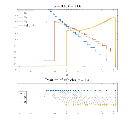
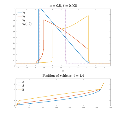
Figure 1. Numerical solutions of (6.1) – (6.3) computed by the explicit Euler scheme. Left: $\ell=0.06$ , right: $\ell=0.005$.

The simulations show that when the speed is determined using weighted Lagrangian coordinates (6.3), vehicles drive faster compared to when the speed is determined by the local FtL model (6.1) or Eulerian coordinates (6.2). This is because the Lagrangian distance between vehicles remains constant even if the Eulerian distance increases. The Lagrangian distance is always less than or equal to the Eulerian distance, giving the Lagrangian model more weight to spacings further ahead. As a result, in a decreasing density or thinly occupied road, the speed determined by the Lagrangian model is greater than or equal to that determined by the Eulerian model.

6.2. The zero-filter ($\alpha\to 0$) limit

We now study the scheme (2.6) for $\alpha=1/2$, $\alpha=1/8$, $\alpha=1/32$ and $\alpha=1/128$ in order to compare $1/w_{\alpha}$ and $1/y_{\alpha}$ with $\rho$, where $\rho$ is the unique entropy solution of the local LWR model

(6.5) $$\partial_{t}\rho+\partial_{x}(\rho V(\rho))=0,\ \ \ \rho(x,0)=\rho_{0}(x).$$

In this setting ($\rho_{0}=\mathrm{const}$ outside an interval $(a,b)$), we define $u_{i}(0)$ and the matrix $\overline{\Phi}_{\alpha}$ as in the previous section and then define the initial data

(6.6) $$y_{i}^{0}=\frac{1}{u_{i}(0)}\ \ \ \text{and}\ \ \ w^{0}_{i}=\sum_{j=i}^{N}\overline{\Phi}_{i,j,\alpha}y^{0}_{j},$$

for $i=1,\ldots,N$. Set ${\Delta z}=\ell$, $\lambda={\Delta t}/{\Delta x}$ where ${\Delta t}$ is chosen such that the CFL-condition (2.7) holds. Let $w^{n}_{i}$ satisfy (2.6), which in this context reads

(6.7) $$w_{i}^{n+1}=w^{n}_{i}+\lambda\Bigl{(}\sum_{j=i+1}^{N}\overline{\Phi}_{i+1,j,\alpha}W\left(w^{n}_{j}\right)-\sum_{j=i+1}^{N}\overline{\Phi}_{i,j,\alpha}W\left(w^{n}_{j}\right)\Bigr{)},$$

for $i=1,\ldots,N$. The scheme for $y^{n}_{i}$ then reads

$$y_{i}^{n+1}=y^{n}_{i}+\lambda\left(W\left(w^{n}_{i+1}\right)-W\left(w^{n}_{i}\right)\right),$$

for $i=1,\ldots,N$. It is not very elucidating to compare $1/y$ and $1/w$ with $\rho$ in Lagrangian coordinates, let therefore the “discrete Eulerian coordinates” $\xi_{i}^{n}$ be defined by

$$\xi^{n}_{1}=x_{1}(0)+{\Delta t}\sum_{m=1}^{n}V\Bigl{(}\,\frac{1}{y^{m}_{1}}\,\Bigr{)},\ \ \ \xi^{n}_{i+1}=\xi^{n}_{i}+y^{n}_{i}{\Delta z},\ \ i=1,\ldots,N-1,$$

cf. (1.3). Hence, we expect that

$$\frac{1}{w^{n}_{i}}\approx\rho(\xi^{n}_{i},t^{n})\ \ \ \text{and}\ \ \ \frac{1}{y^{n}_{i}}\approx\rho(\xi^{n}_{i},t^{n})$$

for sufficiently small $\alpha$.

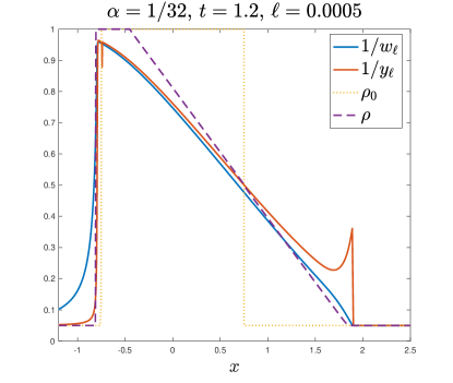
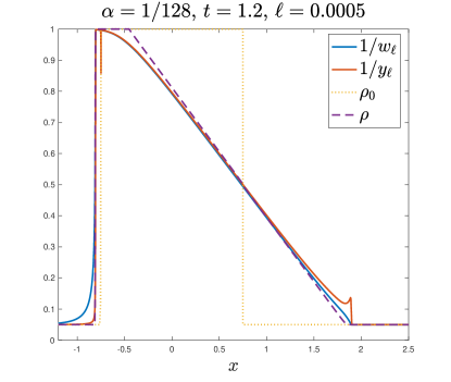
Figure 2. Solutions of (6.7), (6.3),with initial data given in (6.4), (6.6). For all computations $t=1.2$ and $\ell=1/2000$. For comparisons we also show a numerical solution of (6.5). Upper left: $\alpha=1/2$, upper right: $\alpha=1/8$, lower left: $\alpha=1/32$, lower right: $\alpha=1/128$.

In Figure 2 shows $1/w$, $1/y$ and $\rho$ for different values of $\alpha$. In these plots the $x$ axis is the Eulerian coordinates, i.e., we plot the points

$$\left(\xi^{n}_{i},1/w^{n}_{i}\right)\ \ \ \text{and}\ \ \ \left(\xi^{n}_{i},1/y^{n}_{i}\right),$$

for all relevant $i$, and $n$ is such that $t^{n}=1.2$. The approximation to the conservation law (6.5) is computed with the Engquist-Osher scheme on a fine grid. From this figure, we see that $\left\{1/w^{n}_{i}\right\}_{i=1}^{N}$ and $\left\{1/y^{n}_{i}\right\}_{i=1}^{N}$ approach $\left\{\rho(\xi^{n}_{i},t^{n})\right\}_{i=1}^{N}$ in $L^{1}$ as $\alpha$ traverses the sequence $\left\{1/2,1/8,1/32,1/128\right\}$.

6.3. Convergence of $y_{\alpha}$ and the effect of different filters.

We proved that the filter $\Phi=\Phi_{\mathrm{exp}}(z)=e^{-z}$ results in strong convergence of $y_{\alpha}$ to $1/\rho$, the entropy solution of the local LWR conservation law (1.1). This convergence, which followed from $\left\|y_{\alpha}(\cdot,t)-w_{\alpha}(\cdot,t)\right\|_{L^{1}(\mathbb{R})}\lesssim\mathcal{O}(\alpha)$, was also seen in previous experiments. However, this strong convergence has only been proven for this specific filter and may not hold for others. To test this we experimented with other Lipschitz continuous filters:

$$\Phi_{1}(z)=\frac{4}{\pi}\frac{1}{(1+z^{2})^{2}},\ \ \Phi_{\mathrm{tri}}(z)=2\max\left\{1-z,0\right\}\ \ \text{and even}\ \ \Phi_{2}(z)=\frac{2}{\pi}\frac{1}{1+z^{2}},$$

although the last filter is not covered by the theory in this paper. Our numerical experiments show that $y_{\alpha}$ converges strongly for all filters. However, for the discontinuous filter $\Phi_{\mathrm{box}}(z)=\chi_{(0,1)}(z)$, we observe weak convergence oscillations that persist as $\alpha\to 0$.

Oscillatory solutions can be attributed to stop-and-go traffic patterns [28]. Recall that stop-and-go traffic refers to a situation where cars frequently start and stop, resulting in waves of congestion that can propagate through a traffic flow and cause oscillations.

In Figure 3 we compare computations using the initial data (6.4), $\ell=1/5000$, and the filters $\Phi_{\mathrm{tri}}$ (left column) and $\Phi_{\mathrm{box}}$ (right column). In the first row $\alpha=1/32$ and in the second row $\alpha=1/128$.

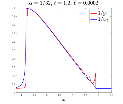
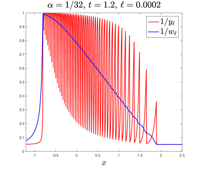
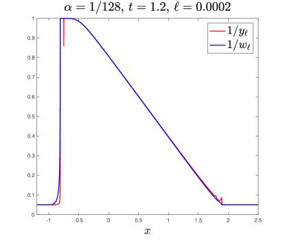
Figure 3. Solutions of (6.7), (6.3),with initial data given in (6.4), (6.6). For all computations $t=1.2$ and $\ell=1/5000$. In the left column, $\Phi=\Phi_{\mathrm{tri}}$, in the right column, $\Phi=\Phi_{\mathrm{box}}$.

From these computations, it is tempting to infer that (at least for these initial data) $y_{\ell}$ converges strongly to $1/\rho$ for the filter $\Phi_{\mathrm{tri}}$ and only weakly to $1/\rho$ for the discontinuous filter $\Phi_{\mathrm{box}}$. To substantiate our suspicion that $y_{\ell}$ only converges weakly, we did one final experiment in which we used the same initial data, but $\ell=1/10000$ and $\alpha=1/256$.

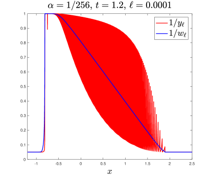
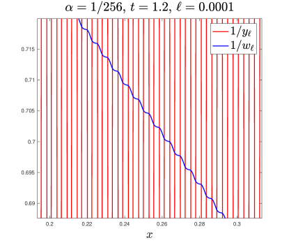
Figure 4. Solutions of (6.7), (6.3),with initial data given in (6.4), (6.6), using the discontinuous filter $\Phi_{\mathrm{box}}$ with $\alpha=1/256$ and $\ell=1/10000$. The figure to the right is just an enlargement of a region of the left figure.

The result is depicted in Figure 4. The right figure is a magnification of the region $x\in[0.2,0.3]$, $\rho\in[0.69,0.72]$ in the left figure.

Our experiment leads us to propose the conjecture that if a filter $\Phi$ is continuous, then the convergence of $y_{\alpha}$ to $1/\rho$ is strong. However, a proof has yet to be provided, except in the case of the exponential filter.

References

• [1] N. Alibaud. Entropy formulation for fractal conservation laws. J. Evol. Equ., 7(1):145–175, 2007.
• [2] N. Alibaud, S. Cifani, and E. R. Jakobsen. Continuous dependence estimates for nonlinear fractional convection-diffusion equations. SIAM J. Math. Anal., 44(2):603–632, 2012.
• [3] S. Blandin and P. Goatin. Well-posedness of a conservation law with non-local flux arising in traffic flow modeling. Numer. Math., 132(2):217–241, 2016.
• [4] A. Bressan and W. Shen. On traffic flow with nonlocal flux: a relaxation representation. Arch. Ration. Mech. Anal., 237(3):1213–1236, 2020.
• [5] A. Bressan and W. Shen. Entropy admissibility of the limit solution for a nonlocal model of traffic flow. Commun. Math. Sci., 19(5):1447–1450, 2021.
• [6] F. A. Chiarello, J. Friedrich, P. Goatin, and S. Göttlich. Micro-macro limit of a nonlocal generalized Aw-Rascle type model. SIAM J. Appl. Math., 80(4):1841–1861, 2020.
• [7] F. A. Chiarello and P. Goatin. Global entropy weak solutions for general non-local traffic flow models with anisotropic kernel. ESAIM Math. Model. Numer. Anal., 52(1):163–180, 2018.
• [8] J. Chien and W. Shen. Stationary wave profiles for nonlocal particle models of traffic flow on rough roads. NoDEA Nonlinear Differential Equations Appl., 26(6):Paper No. 53, 25, 2019.
• [9] G. M. Coclite, J.-M. Coron, N. De Nitti, A. Keimer, and L. Pflug. A general result on the approximation of local conservation laws by nonlocal conservation laws: the singular limit problem for exponential kernels. Ann. Inst. H. Poincaré C Anal. Non Linéaire, 40(5):1205–1223, 2023.
• [10] G. M. Coclite, N. De Nitti, A. Keimer, and L. Pflug. On existence and uniqueness of weak solutions to nonlocal conservation laws with BV kernels. Z. Angew. Math. Phys., 73(6):10, 2022. Id/No 241.
• [11] M. Colombo, G. Crippa, E. Marconi, and L. V. Spinolo. Local limit of nonlocal traffic models: convergence results and total variation blow-up. Ann. Inst. H. Poincaré C Anal. Non Linéaire, 38(5):1653–1666, 2021.
• [12] M. Colombo, G. Crippa, E. Marconi, et al. Nonlocal traffic models with general kernels: singular limit, entropy admissibility, and convergence rate. Arch. Ration. Mech. Anal., 247(18), 2023.
• [13] C. M. Dafermos. Hyperbolic conservation laws in continuum physics. Springer-Verlag, Berlin, third edition, 2010.
• [14] M. Di Francesco and M. D. Rosini. Rigorous derivation of nonlinear scalar conservation laws from follow-the-leader type models via many particle limit. Arch. Ration. Mech. Anal., 217(3):831–871, 2015.
• [15] J. Friedrich, O. Kolb, and S. Göttlich. A Godunov type scheme for a class of LWR traffic flow models with non-local flux. Netw. Heterog. Media, 13(4):531–547, 2018.
• [16] P. Goatin and S. Scialanga. Well-posedness and finite volume approximations of the LWR traffic flow model with non-local velocity. Netw. Heterog. Media, 11(1):107–121, 2016.
• [17] H. Holden and N. H. Risebro. Front tracking for hyperbolic conservation laws, volume 152 of Applied Mathematical Sciences. Springer, Heidelberg, second edition, 2015.
• [18] H. Holden and N. H. Risebro. The continuum limit of Follow-the-Leader models—a short proof. Discrete Contin. Dyn. Syst., 38(2):715–722, 2018.
• [19] K. H. Karlsen and S. Ulusoy. Stability of entropy solutions for Lévy mixed hyperbolic-parabolic equations. Electron. J. Differential Equations, 2011(116):1–23, 2011.
• [20] A. Keimer and L. Pflug. On approximation of local conservation laws by nonlocal conservation laws. J. Math. Anal. Appl., 475(2):1927–1955, 2019.
• [21] S. N. Kružkov. First order quasilinear equations with several independent variables. Mat. Sb. (N.S.), 81 (123):228–255, 1970.
• [22] L. Leclercq, J. A. Laval, and E. Chevallier. The Lagrangian coordinates and what it means for first order traffic flow models. 2007.
• [23] M. J. Lighthill and G. B. Whitham. On kinematic waves. II. A theory of traffic flow on long crowded roads. Proc. Roy. Soc. London Ser. A, 229:317–345, 1955.
• [24] J. Ridder and W. Shen. Traveling waves for nonlocal models of traffic flow. Discrete Contin. Dyn. Syst., 39(7):4001–4040, 2019.
• [25] K.-i. Sato. Lévy processes and infinitely divisible distributions, volume 68 of Cambridge Studies in Advanced Mathematics. Cambridge University Press, Cambridge, 1999.
• [26] W. Shen and K. Shikh-Khalil. Traveling waves for a microscopic model of traffic flow. Discrete Contin. Dyn. Syst., 38(5):2571–2589, 2018.
• [27] J. M. Steele. The Cauchy-Schwarz master class. AMS/MAA Problem Books Series. Mathematical Association of America, Washington, DC; Cambridge University Press, Cambridge, 2004. An introduction to the art of mathematical inequalities.
• [28] M. Treiber and A. Kesting. Traffic flow dynamics. Springer, Heidelberg, 2013. Data, models and simulation, Translated by Treiber and Christian Thiemann.
• [29] D. H. Wagner. Equivalence of the Euler and Lagrangian equations of gas dynamics for weak solutions. J. Differential Equations, 68(1):118–136, 1987.