On Generalized Degree Fairness in Graph Neural Networks

Abstract

Conventional graph neural networks (GNNs) are often confronted with fairness issues that may stem from their input, including node attributes and neighbors surrounding a node. While several recent approaches have been proposed to eliminate the bias rooted in sensitive attributes, they ignore the other key input of GNNs, namely the neighbors of a node, which can introduce bias since GNNs hinge on neighborhood structures to generate node representations. In particular, the varying neighborhood structures across nodes, manifesting themselves in drastically different node degrees, give rise to the diverse behaviors of nodes and biased outcomes. In this paper, we first define and generalize the degree bias using a generalized definition of node degree as a manifestation and quantification of different multi-hop structures around different nodes. To address the bias in the context of node classification, we propose a novel GNN framework called Generalized Degree Fairness-centric Graph Neural Network (DegFairGNN). Specifically, in each GNN layer, we employ a learnable debiasing function to generate debiasing contexts, which modulate the layer-wise neighborhood aggregation to eliminate the degree bias originating from the diverse degrees among nodes. Extensive experiments on three benchmark datasets demonstrate the effectiveness of our model on both accuracy and fairness metrics.

1 Introduction

Graph neural networks (GNNs) (Kipf and Welling 2017; Hamilton, Ying, and Leskovec 2017; Veličković et al. 2018) have emerged as a powerful family of graph representation learning approaches. They typically adopt a message passing framework, in which each node on the graph aggregates information from its neighbors recursively in multiple layers, unifying both node attributes and structures to generate node representations. Despite their success, GNNs are often confronted with fairness issues stemming from input node attributes (Zemel et al. 2013; Dwork et al. 2012). To be more specific, certain sensitive attributes (e.g., gender, age or race) may trigger bias and cause unfairness in downstream applications. Naïvely removing the sensitive attributes does not adequately improve fairness, as the correlation between sensitive attributes and other attributes could still induce bias (Pedreshi, Ruggieri, and Turini 2008). Thus, prior work on Euclidean data often employs additional regularizations or constraints to debias the model or post-processing the predictions (Hardt, Price, and Srebro 2016; Pleiss et al. 2017). Similar principles have been extended to graphs to eliminate bias rooted in sensitive node attributes (Rahman et al. 2019; Bose and Hamilton 2019; Buyl and De Bie 2020; Li et al. 2021; Dai and Wang 2021; Wang et al. 2022). For example, CFC (Bose and Hamilton 2019) tries to debias by applying some filters on the generated node representations, and some others resort to adversarial learning to detect sensitive attributes (Bose and Hamilton 2019; Dai and Wang 2021).

However, these approaches fail to account for the other key input of GNNs—the neighborhood structures of each node, which can also induce bias into node representations. Specifically, each node is linked to different neighbors, forming diverse neighborhood structures and manifesting drastically different node degrees. By virtue of the message passing framework, GNNs generate the representation of a node based on its neighborhood structures, which is highly dependent on the abundance or scarcity of its neighboring nodes. Hence, drastic differences in node degrees could lead to differential node behaviors and biased outcomes. In particular, while the “value” of a node is usually co-determined by its own attributes and its neighboring structure (i.e., “social capital”), the latter may systematically bias against newcomers despite their individual attributes, and established individuals may passively accumulate more social capital and become even harder for newcomers to compete. For example, on a social network involving NBA players (Dai and Wang 2021), a player with more followers may command a higher salary than another player with comparable physical ability and skills due to his popularity among fans; in a citation network, a paper with more initial citations may attract even more future citations than another paper with comparable quality on the same topic. Generally, a node of larger degree is more likely to possess crucial advantages and thus receives more favorable outcomes than warranted. This reveals a notable issue of degree fairness, in which the degree-biased neighborhood structures can marginalize or even override the quality and competency of individual nodes. The goal of degree fairness is to achieve equitable outcomes for nodes of different degrees, such that individuals of comparable competency should receive similar outcomes. More generally, we can also consider the degree bias stemming from multi-hop structures surrounding a node, using a generalized definition of node degrees.

In this paper, we investigate the important problem of degree fairness in graph neural networks in the context of node classification, which has not been explored to date. On one hand, simply employing neighborhood sampling cannot address this issue due to the potential correlation between node attributes and their structures, and may further result in information loss (Wu, He, and Xu 2019; Tang et al. 2020; Liu, Nguyen, and Fang 2021). On the other hand, node degree is a manifestation of neighborhood structures, which is fundamentally different from a sensitive node attribute (Rahman et al. 2019; Bose and Hamilton 2019; Li et al. 2021; Dai and Wang 2021). Particularly, in GNNs each node receives information from its neighbors, and thus nodes of diverse degrees can access varying amount of information, giving rise to the degree bias in learnt representations. Moreover, the bias may be further amplified by multi-layered recursive neighborhood aggregation in GNNs. While existing debiasing approaches that directly filter node representations are plausible for attribute-oriented fairness, they do not debias the core operation of neighborhood aggregation and thus cannot fundamentally alleviate the degree bias intrinsic to the diverse neighborhood structures.

Toward degree fairness, we first introduce generalized degree to quantify the abundance or scarcity of multi-hop contextual structures for each node, since in a broader sense the degree bias of a node stems not only from its one-hop neighborhood, but also its local context within a few hops. We further propose a novel generalized Degree Fairness-centric GNN framework named DegFairGNN, which can work with any neighborhood aggregation-based GNN architecture. To fundamentally address degree fairness, we employ a learnable debiasing function to generate different debiasing contexts, which are meant to balance the structural contrast between nodes with high and low generalized degrees. Specifically, the debiasing contexts directly target the neighborhood aggregation operation in each GNN layer, aiming to complement the neighborhood of low-degree nodes, while distilling the neighborhood of high-degree nodes. As a result, the drastic differences in contextual structures across nodes can be balanced to reach a structurally fair state, enabling the generation of fair node representations.

To summarize, our contributions are three-fold. (1) We make the first attempt on defining and addressing generalized degree fairness in GNNs. (2) We propose a novel generalized degree fairness-centric GNN framework named DegFairGNN that can flexibly work with neighborhood aggregation-based GNNs, to eliminate the generalized degree bias rooted in the layer-wise neighborhood aggregation. (3) Extensive experiments demonstrate that our proposed model is effective in both fairness and accuracy metrics.

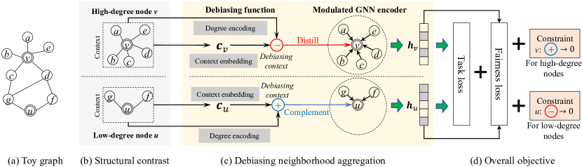
Figure 1: Overall framework of DegFairGNN.

2 Problem Formulation

In this section, we introduce the definition of generalized degree fairness on graphs and several related concepts.

Graph. A graph is given by $\mathcal{G}=\{\mathcal{V},\mathcal{E},\mathbf{X}\}$, where $\mathcal{V}$ is the set of nodes, $\mathcal{E}$ is the set of edges, and $\mathbf{X}\in\mathbb{R}^{|\mathcal{V}|\times d_{X}}$ is the node attribute matrix with $d_{X}$ equalling the number of attributes. Equivalently, $\mathbf{x}_{v}\in\mathbb{R}^{d_{X}}$ is the attribute vector of node $v$. Let $\mathbf{A}\in\mathbb{R}^{|\mathcal{V}|\times|\mathcal{V}|}$ denote the corresponding adjacency matrix of $\mathcal{G}$.

Generalized degree. In a broader sense, the degree bias on a node stems not only from its (one-hop) neighborhood, but also its local context within a certain number of hops. Formally, the $r$-hop local context of node $v$ is defined as $\mathcal{C}_{r}=\{v^{\prime}\in\mathcal{V}\mid d(v,v^{\prime})\leq r\}$, i.e., the set of nodes reachable from $v$ in at most $r$ steps, where $d(\cdot,\cdot)$ is the shortest distance from $v$ to $v^{\prime}$ on the graph. Subsequently, we introduce generalized degree to quantify the abundance of multi-hop local context surrounding a node. Given a node $v$, we define its $r$-hop generalized degree $\deg_{r}(v)\in\mathbb{R}$ as

$$\deg_{r}(v)=[\mathbf{A}^{r}\mathbf{1}]_{v},$$ (1)

where $r\in\mathbb{N}^{+}$ is the number of hops, $\mathbf{1}\in\mathbb{R}^{|\mathcal{V}|}$ is a column vector filled with ones, and $[\mathbf{x}]_{i}$ denotes the $i$-th entry in vector $\mathbf{x}$. Here $[\mathbf{A}^{r}]_{i,j}$, the $(i,j)$ entry in the matrix $\mathbf{A}^{r}$, gives the number of walks of length $r$ from node $i$ to node $j$. Thus, $\deg_{r}(v)$ represents the total number of (non-distinct) nodes reachable from $v$ in $r$ hops, a straightforward measure of the abundance of $v$’s $r$-hop local context. As a special case, $\deg_{1}(v)$ is simply the (1-hop) degree of $v$.

Generalized degree fairness. Generalized degree fairness amounts to node representations that are free from variant generalized degrees. In the context of multi-class node classification, we formalize two fairness definitions in terms of statistical parity (Dwork et al. 2012) and equal opportunity (Hardt, Price, and Srebro 2016). Both definitions rely on the notion of generalized degree groups, in which we divide the nodes into $m$ mutually exclusive groups $\mathcal{G}_{1},\ldots,\mathcal{G}_{m}$ so that

$$\mathcal{G}_{i}=\{v\in\mathcal{V}\mid d_{i}\leq\deg_{r}(v)<d_{i+1}\},$$ (2)

where $d_{1}<d_{2}<\ldots<d_{m+1}$ are a series of degree boundaries between the groups, and $d_{1}=\min_{v\in\mathcal{V}}\deg_{r}(v)$ and $d_{m+1}=\max_{v\in\mathcal{V}}\deg_{r}(v)+1$. Furthermore, let $\mathcal{Y}$ be the set of classes. For ease of discussion, hereafter we may simply call “generalized degree” as “degree”.

To achieve Degree Statistical Parity (DSP), we require the class predictions to be independent of node degree groups. That is, for any class $y\in\mathcal{Y}$ and any two groups $\mathcal{G}_{i}$ and $\mathcal{G}_{j}$,

$$P(\hat{y}_{v}=y|v\in\mathcal{G}_{i})=P(\hat{y}_{v}=y|v\in\mathcal{G}_{j}),$$ (3)

where $\hat{y}_{v}$ is the predicted class of $v$. To achieve Degree Equal Opportunity (DEO), we require the probability of each node being predicted into its true class $y$ to be equal for nodes in different degree groups. That is,

$$P(\hat{y}_{v}=y|y_{v}=y,v\in\mathcal{G}_{i})\vspace{-4mm}=\vspace{-4mm}P(\hat{y}_{v}=y|y_{v}=y,v\in\mathcal{G}_{j}),$$

where $y_{v}$ is the true class of $v$.

Our degree fairness is defined in a group-wise manner, which is in line with existing fairness definitions (Zafar et al. 2017; Agarwal, Lakkaraju, and Zitnik 2021) and offers a flexible setup. On the one hand, a simple and practical scenario could involve just two groups, since typically the degree fairness issue is the most serious between nodes with the smallest and largest degrees. On the other hand, the most fine-grained groups would be each unique value of degree forming its own group, but it is not ideal for two reasons. First, some groups may have very few nodes depending on the degree distribution, leading to large variance. Second, the smoothness of degrees are lost: nodes of similar degrees are expected to have rather similar advantage or disadvantage compared to nodes of very different degrees.

3 Proposed Model: DegFairGNN

In this section, we introduce the proposed DegFairGNN, starting with some preliminaries on GNNs.

3.1 Preliminaries on GNNs

Modern GNNs usually resort to multi-layer neighborhood aggregation, in which each node recursively aggregates information from its neighbors. Specifically, in the $l$-th layer the representation of node $v$, $\mathbf{h}^{l}_{v}\in\mathbb{R}^{d_{l}}$, is constructed as

$$\mathbf{h}^{l}_{v}=\sigma\left(\textsc{Aggr}\left(\{\mathbf{h}^{l-1}_{u}\mid u\in\mathcal{N}_{v}\};\omega^{l}\right)\right),$$ (4)

where $d_{l}$ is the dimension of node representations in the $l$-th layer, $\textsc{Aggr}(\cdot)$ denotes an aggregation function such as mean-pooling (Kipf and Welling 2017) or self-attention (Veličković et al. 2018), $\sigma$ is an activation function, $\mathcal{N}_{v}$ denotes the set of neighbors of $v$, and $\omega^{l}$ denotes the learnable parameters in layer $l$. Node representations in the input layer are given by the input node attributes, i.e., $\mathbf{h}^{0}_{v}\equiv\mathbf{x}_{v}$.

3.2 Overall Framework

The overall framework of DegFairGNN is illustrated in Fig. 1. We first design a strategy of structural contrast in Fig. 1(b), to split nodes into two groups by their degree. The two groups contrast each other to facilitate the learning of a debiasing function, which generates node-specific debiasing contexts to modulate neighborhood aggregation, as shown in Fig. 1(c). More specifically, the modulation aims to distill high-degree nodes to remove bias, and complement low-degree nodes to enrich their degree-biased neighborhood structures. Thus, by trying to balance the two groups, the modulation is able to debias neighborhood aggregation. Finally, the debiasing function and GNN are jointly optimized by the task loss and the fairness loss in Fig. 1(d).

3.3 Structural Contrast

To debias nodes with varying contextual structures, we propose to learn the debiasing function by contrasting between two groups of nodes, namely, low-degree nodes $\mathcal{S}_{0}$ and high-degree nodes $\mathcal{S}_{1}$, as illustrated in Fig. 1(b). Note that in the layer-wise neighborhood aggregation in Eq. (4), each node can only access its one-hop local contexts in each layer. Thus, it is a natural choice to construct the two groups based on one-hop degree: $\mathcal{S}_{0}=\{v\in\mathcal{V}\mid\deg_{1}(v)\leqslant K\}$ and $\mathcal{S}_{1}=\mathcal{V}\setminus\mathcal{S}_{0}$. That is, $\mathcal{S}_{0}$ is the low-degree group, $\mathcal{S}_{1}$ is the high-degree group, and $K$ is a threshold hyperparameter. Note that having two groups can provide the most significant contrast for model training.

To contrast between the two groups, nodes in the same group would share the learnable parameters for the debiasing mechanism, whereas nodes across different groups would have different parameters. This strategy enables the two groups to eliminate the degree bias in different ways, which is desirable given their different degrees.

3.4 Debiasing Neighborhood Aggregation

To fundamentally eliminate degree bias, we propose to debias neighborhood aggregation, the key operation in GNNs in which degree bias is rooted. As shown in Fig. 1(c), we leverage a learnable debiasing function to generate the debiasing contexts, which modulate the neighborhood aggregation for each node and in each layer of the GNN encoder.

Debiasing function. More concretely, we leverage a debiasing function $\mathcal{D}(\cdot)$ with learnable parameters to fit each group, due to the divergence between the two groups in terms of node degree. On one hand, for a low-degree node $u\in\mathcal{S}_{0}$, $\mathcal{D}(u;\theta^{l}_{0})\in\mathbb{R}^{d_{l}}$ outputs the debiasing context for $u$ in layer $l$ to complement the neighborhood of $u$. On the other hand, for a high-degree node $v\in\mathcal{S}_{1}$, $\mathcal{D}(v;\theta^{l}_{1})\in\mathbb{R}^{d_{l}}$ outputs the debiasing context for $v$ in layer $l$ to distill the neighborhood of $v$. Note that each group $\mathcal{S}_{*}$ has its own parameters $\theta^{l}_{*}$ for $\mathcal{D}(\cdot)$ in layer $l$. The learning is guided by a fairness loss in the overall objective (see Sect. 3.5), which drives the debiasing contexts toward distilling information on the high-degree nodes while complementing information on the low-degree nodes, in order to achieve the balance and fairness between the two groups.

The debiasing function is designed to generate a debiasing context for each node in each layer, to modulate the neighborhood aggregation in a node- and layer-wise manner. To achieve ideal modulations, the debiasing contexts should be comprehensive and adaptive.

Comprehensiveness. First, debiasing contexts need to be comprehensive, to account for both the content and structure information in the neighborhood. To be comprehensive, we resort to the context embedding of node $v$ in layer $l$, denoted $\mathbf{c}^{l}_{v}\in\mathbb{R}^{d_{l-1}}$, which can be calculated as

$$\mathbf{c}^{l}_{v}=\textsc{Pool}(\{\mathbf{h}^{l-1}_{u}\mid u\in\mathcal{C}_{r}(v)\}),$$ (5)

where $\textsc{Pool}(\cdot)$ is a pooling function. Here we use a simple mean pooling, although it can also be made learnable. The context embedding $\mathbf{c}^{l}_{v}$ aggregates the layer-($l$-$1$) contents in node $v$’s $r$-hop local context $\mathcal{C}_{r}(v)$, and thus embodies both the content and structure information. The debiasing function is then a function of the context embedding, i.e.,

$$\mathcal{D}(v;\theta^{l}_{*})=f(\mathbf{c}^{l}_{v};\theta^{l}_{c,*}),$$ (6)

which is parameterized by $\theta^{l}_{c,*}$, where $*$ is $0$ or $1$ depending on the node group. We use a fully connected layer as $f$.

Adaptiveness. Second, debiasing contexts need to be adaptive, to sufficiently customize to each node. While the two groups of nodes, $\mathcal{S}_{0}$ and $\mathcal{S}_{1}$, are already differentiated by group-specific parameters for the debiasing function, the differentiation is coarse-grained and cannot sufficiently adapt to individual nodes. In particular, even for nodes in the same group, their degrees still vary, motivating the need for finer-grained node-wise adaptation. However, letting each node have node-specific parameters is not feasible due to a much larger model size, which tends to cause overfitting and scalability issues. For fine-grained adaptation without blowing up the model size, inspired by hypernetworks (Ha, Dai, and Le 2017; Perez et al. 2018; Liu et al. 2021), we adopt a secondary neural network to generate node-wise transformations on the debiasing contexts in each layer. Concretely, the debiasing function can be reformulated as

$$\mathcal{D}(v;\theta^{l}_{*})=(\gamma^{l}_{v}+\mathbf{1})\odot f(\mathbf{c}^{l}_{v};\theta^{l}_{c,*})+\beta^{l}_{v},$$ (7)

where $\gamma^{l}_{v}$ and $\beta^{l}_{v}\in\mathbb{R}^{d_{l}}$ are node-specific scaling and shifting operators in layer $l$, respectively. Here $\odot$ denotes element-wise multiplication, and $\mathbf{1}$ is a vector of ones to ensure that the scaling is centered around one. Note that $\gamma^{l}_{v}$ and $\beta^{l}_{v}\in\mathbb{R}^{d_{l}}$ are not directly learnable, but are respectively generated by a secondary network conditioned on each node’s degree. Specifically,

$$\gamma^{l}_{v}=\phi_{\gamma}(\delta^{l}(v);\theta^{l}_{\gamma}),\quad\beta^{l}_{v}=\phi_{\beta}(\delta^{l}(v);\theta^{l}_{\beta}),$$ (8)

where $\phi_{\gamma}$ and $\phi_{\beta}$ can be any neural network, and we simply use a fully connected layer. The input to these secondary networks, $\delta^{l}(v)$, is the degree encoding of $v$ to condition the transformations on the degree of $v$, which we will elaborate later. Thus, the learnable parameters of the debiasing function in Eq. (7) become $\theta^{l}_{*}=\{\theta^{l}_{c,*},\theta^{l}_{\gamma},\theta^{l}_{\beta}\}$ in layer $l$, and $\theta_{*}=\{\theta^{1}_{*},\theta^{2}_{*},\ldots\}$ denotes the full set of learnable parameters of the debiasing function for nodes in group $\mathcal{S}_{*}$.

Finally, the input to the secondary network in Eq. (8) is the degree encoding $\delta^{l}(v)$, instead of the degree of $v$ itself. The reason is that degree is an ordinal variable, implicating that degree-conditioned functions should be smooth w.r.t. small changes in degree. In other words, nodes with similar degrees should undergo similar transformations, and vice versa. In light of this, inspired by positional encoding (Vaswani et al. 2017), we propose to encode the degree of a node $v$ in layer $l$ into a vector $\delta^{l}(v)\in\mathbb{R}^{d_{l}}$, such that $[\delta^{l}(v)]_{2i}=\sin(\deg_{1}(v)/10000^{2i/d_{l}})$ and $[\delta^{l}(v)]_{2i+1}=\cos(\deg_{1}(v)/10000^{2i/d_{l}})$. Note that, although nodes at the periphery of the two groups $\mathcal{S}_{0}$ and $\mathcal{S}_{1}$ (e.g., nodes with degrees $K$ and $K+1$) have different debiasing parameters ($\theta_{c,0}$ and $\theta_{c,1}$), the usage of degree encoding in Eqs. (7) and (8) will assimilate their debiasing contexts to some extent given their similar degrees.

Modulated GNN encoder. Given the debiasing contexts, we couple it with the standard neighborhood aggregation in Eq. (4), and modulate neighborhood aggregation for the two groups differently. Specifically, in layer $l$,

$$\mathbf{h}^{l}_{v}=\sigma\bigg{(}\textsc{Aggr}(\{\mathbf{h}^{l-1}_{u}\mid u\in\mathcal{N}_{v}\};\omega^{l})$$

$$+\epsilon\cdot\big{(}\underbrace{I(v\in\mathcal{S}_{0})\mathcal{D}(v;\theta^{l}_{0})}_{\text{complement low-deg.~{}group}}+\underbrace{I(v\in\mathcal{S}_{1})\mathcal{D}(v;\theta^{l}_{1})}_{\text{distill high-deg.~{}group}}\big{)}\bigg{)},$$ (9)

where $I(\cdot)$ is a 0/1 indicator function based on the truth value of its argument, and $\epsilon>0$ is a hyperparameter to control the impact of the debiasing contexts.

3.5 Training Constraints and Objective

We focus on the task of node classification. Apart from the classification loss and the fairness loss associated with the classification, we further introduce several useful constraints to improve the training process, as shown in Fig. 1(d).

Classification loss. For node classification, the last layer of the GNN typically sets the dimension to the number of classes, and uses a softmax activation such that the $i$-th output dimension is the probability of class $i$. With a total of $\ell$ layers, the output node representations $\{\mathbf{h}^{\ell}_{v}:v\in\mathcal{V}^{\text{tr}}\}$ of the training nodes $\mathcal{V}^{\text{tr}}$ can be fed into the cross-entropy loss,

$$\mathcal{L}_{1}=- \textstyle\sum_{v\in\mathcal{V}^{\text{tr}}}\sum_{y=1}^{|\mathcal{Y}|}[\mathbf{y}_{v}]_{y}\ln[\mathbf{h}^{\ell}_{v}]_{y},$$ (10)

where $\mathbf{y}_{v}$ is the one-hot vector of $v$’s class.

Fairness loss. As the proposed debiasing function in Eq. (7) is learnable, it should be driven toward fair representations. Thus, we further employ a fairness loss on the training data. Let $\mathcal{S}_{0}^{\text{tr}}$ and $\mathcal{S}_{1}^{\text{tr}}$ denote the group of low- and high-degree nodes in the training data, respectively. We use a DSP-based loss, trying to achieve parity in the predicted probabilities for the two groups, as follows.

$$\mathcal{L}_{2}=\textstyle\left\|{\textstyle\frac{1}{|\mathcal{S}_{0}^{\text{tr}}|}}\sum_{v\in\mathcal{S}_{0}^{\text{tr}}}\mathbf{h}^{\ell}_{v}-{\textstyle\frac{1}{|\mathcal{S}_{1}^{\text{tr}}|}}\sum_{v\in\mathcal{S}_{1}^{\text{tr}}}\mathbf{h}^{\ell}_{v}\right\|^{2}_{2},$$ (11)

where $\|\cdot\|^{2}_{2}$ is the $L_{2}$ norm. This fairness loss drives the learnable debiasing function toward the fairness metric (e.g., DSP here) to guide the training of DegFairGNN, by constraining the debiasing function to learn how to distill information on high-degree nodes and complement information on low-degree nodes, respectively. Besides, it is also possible to apply DEO. Note that, the fairness loss aims to constrain the prediction distribution to be similar across the two groups, yet does not require the node representations to be similar. Thus, DegFairGNN would not worsen the over-smoothing phenomenon (Xu et al. 2018).

Constraints on debiasing contexts. For a low-degree node $u$, its debiasing context $\mathcal{D}(u;\theta^{l}_{0})$ aims to complement but not distill its neighborhood. On the contrary, for a high-degree node $v$, its debiasing context $\mathcal{D}(v;\theta^{l}_{1})$ aims to distill but not complement its neighborhood. Thus, both $\mathcal{D}(\cdot;\theta^{l}_{1})$ for low-degree nodes in $\mathcal{S}_{0}$ and $\mathcal{D}(\cdot;\theta^{l}_{0})$ for high-degree nodes in $\mathcal{S}_{1}$ should be close to zero. The two constraints promote the learning of debiasing contexts by contrasting between the two groups, which can be formulated as the following loss.

$$\mathcal{L}_{3}=\sum_{l=1}^{\ell}\bigg{(}\sum_{v\in\mathcal{S}_{0}^{\text{tr}}}\|\mathcal{D}(v;\theta^{l}_{1})\|^{2}_{2}+\sum_{v\in\mathcal{S}_{1}^{\text{tr}}}\|\mathcal{D}(v;\theta^{l}_{0})\|^{2}_{2}\bigg{)}.$$ (12)

Constraints on scaling and shifting. To prevent overfitting the data with arbitrarily large scaling and shifting, we further consider the loss below to restrict the search space.

$$\mathcal{L}_{4}=\textstyle\sum_{l=1}^{\ell}\sum_{v\in\mathcal{V}^{\text{tr}}}(\|\gamma^{l}_{v}\|^{2}_{2}+\|\beta^{l}_{v}\|^{2}_{2}).$$ (13)

Overall loss. By combining all the above loss terms, we formulate the overall loss as

$$\mathcal{L}=\mathcal{L}_{1}+\mu\mathcal{L}_{2}+\lambda(\mathcal{L}_{3}+\mathcal{L}_{4}),$$ (14)

where $\mu,\lambda$ are hyper-parameters. In Appendix A, we outline the training procedure and give a complexity analysis.

4 Experiments

In this section, we evaluate the proposed DegFairGNNin terms of both accuracy and fairness.

4.1 Experimental Setup

Datasets. We use two Wikipedia networks, Chameleon and Squirrel (Pei et al. 2020), in which each node represents a Wikipedia page, and each edge denotes a reference between two pages in either direction. We split the nodes into five categories w.r.t. their traffic volume for classification. We also use a citation network EMNLP (Ma et al. 2021), in which each node denotes a paper published in the conference, and each edge denotes two papers that have been co-cited. We split the nodes into two categories w.r.t. their out-of-EMNLP citation count for classification. We summarize the datasets in Table 1, and present more details in Appendix B. Note that, both traffic volumes and citation counts can be deemed as individual benefits of the nodes that tend to be biased by the node degree, motivating us to employ these datasets. In these contexts, a GNN that predicts the benefit outcome independently of degree groups is trying to be fair, which should focus on the relevance and quality of the nodes rather than their existing links.

Table 1: Summary of datasets.

Dataset	Nodes	Edges	Features	Classes
Chameleon	2,277	31,371	2,325	5 (traffic volume)
Squirrel	5,201	198,353	2,089	5 (traffic volume)
EMNLP	2,600	7,969	8	2 (citation count)

Base GNNs. Our proposed DegFairGNN can work with different GNN backbones. We employ GCN (Kipf and Welling 2017) as the default base GNN in our experiments, and name the corresponding fairness model DegFairGCN. We also adopt two other base GNNs, GAT (Veličković et al. 2018) and GraphSAGE (Hamilton, Ying, and Leskovec 2017), as described in Appendix C.

Baselines. We consider the following two categories of baselines. (1) Degree-specific models: DSGCN (Tang et al. 2020), Residual2Vec (Kojaku et al. 2021) and Tail-GNN (Liu, Nguyen, and Fang 2021). They employ degree-specific operations on the nodes w.r.t. their degrees, to improve task accuracy especially for the low-degree nodes. (2) Fairness-aware models: FairWalk (Rahman et al. 2019), CFC (Bose and Hamilton 2019), FairGNN (Dai and Wang 2021), FairAdj (Li et al. 2021) and FairVGNN (Wang et al. 2022). They are proposed to address the sensitive attribute-based fairness of nodes on graphs. To apply them to degree fairness, we define the generalized node degree as the sensitive attribute. However, even so, these fairness-aware baselines do not debias the neighborhood aggregation mechanism in each GNN layer, and thus fall short of addressing the degree bias from the root. More details of the baselines are given in Appendix D.

Data split and parameters. For all the datasets, we randomly split the nodes into training, validation and test set with proportion 6:2:2. We set the threshold $K$ for the structural contrast in Sect. 3.3 as the mean node degree by default. We further analyze the impact of $K$ on both accuracy and fairness in Appendix G.2. For other hyper-parameter settings, please refer to Appendix E.

Table 2: Comparison with baselines ($r=1$, 20% Top/Bottom).

Henceforth, tabular results are in percent with standard deviation over 5 runs; the best fairness result is bolded and the runner-up is underlined. GCN DSGCN Residual2Vec Tail-GNN FairWalk CFC FairGNN FairAdj FairVGNN DegFairGCN Chamel. Acc. $\uparrow$ 62.45 $\pm$ 0.21 63.90 $\pm$ 1.28 49.04 $\pm$ 0.01 66.08 $\pm$ 0.19 56.36 $\pm$ 0.75 63.02 $\pm$ 0.84 70.70 $\pm$ 0.52 51.71 $\pm$ 1.13 72.32 $\pm$ 0.50 69.91 $\pm$ 0.19 $\Delta_{\text{DSP}}\downarrow$   9.68 $\pm$ 1.37   8.81 $\pm$ 1.15 14.52 $\pm$ 0.69   8.51 $\pm$ 1.72   8.18 $\pm$ 0.93 10.12 $\pm$ 1.28   7.33 $\pm$ 1.09   9.79 $\pm$ 1.91   8.86 $\pm$ 1.11   5.85 $\pm$ 0.32 $\Delta_{\text{DEO}}\downarrow$ 36.08 $\pm$ 2.65 25.14 $\pm$ 2.67 37.31 $\pm$ 1.99 26.09 $\pm$ 3.25 22.89 $\pm$ 2.75 29.54 $\pm$ 1.95 26.83 $\pm$ 1.95 27.48 $\pm$ 2.06 26.02 $\pm$ 2.39 21.60 $\pm$ 0.71 Squirrel Acc. $\uparrow$ 47.85 $\pm$ 1.33 40.71 $\pm$ 2.17 28.47 $\pm$ 0.01 42.62 $\pm$ 0.06 37.68 $\pm$ 0.65 45.64 $\pm$ 2.19 57.29 $\pm$ 0.77 35.18 $\pm$ 1.22 46.97 $\pm$ 0.48 59.21 $\pm$ 0.97 $\Delta_{\text{DSP}}\downarrow$ 13.37 $\pm$ 2.83 16.08 $\pm$ 0.86 25.11 $\pm$ 0.48 18.91 $\pm$ 0.26   7.94 $\pm$ 0.36 12.40 $\pm$ 0.48 12.96 $\pm$ 1.03 16.63 $\pm$ 1.56 26.67 $\pm$ 0.52   9.54 $\pm$ 1.02 $\Delta_{\text{DEO}}\downarrow$ 27.00 $\pm$ 3.79 32.61 $\pm$ 3.74 34.49 $\pm$ 0.72 33.60 $\pm$ 0.72 17.12 $\pm$ 1.50 21.60 $\pm$ 2.69 17.62 $\pm$ 2.40 27.54 $\pm$ 1.73 35.80 $\pm$ 1.76 16.42 $\pm$ 1.38 EMNLP Acc. $\uparrow$ 78.92 $\pm$ 0.43 82.19 $\pm$ 0.77 80.69 $\pm$ 0.01 83.72 $\pm$ 0.28 82.23 $\pm$ 0.18 80.15 $\pm$ 1.13 86.81 $\pm$ 0.22 76.50 $\pm$ 1.55 84.03 $\pm$ 0.34 79.92 $\pm$ 0.77 $\Delta_{\text{DSP}}\downarrow$ 44.55 $\pm$ 1.90 50.00 $\pm$ 2.98 12.90 $\pm$ 0.15 41.18 $\pm$ 1.58 33.52 $\pm$ 1.46 56.60 $\pm$ 1.95 58.23 $\pm$ 1.44 40.38 $\pm$ 4.64 43.92 $\pm$ 1.43 12.38 $\pm$ 3.72 $\Delta_{\text{DEO}}\downarrow$ 34.05 $\pm$ 3.56 46.92 $\pm$ 2.91 11.26 $\pm$ 0.67 36.76 $\pm$ 1.48 30.67 $\pm$ 1.42 45.21 $\pm$ 2.27 51.56 $\pm$ 1.38 41.89 $\pm$ 4.78 40.95 $\pm$ 1.71   8.52 $\pm$ 2.26

Evaluation. For model performance, we evaluate the node classification accuracy on the test set.

For model fairness, the group-wise DSP and DEO (Sect. 2) essentially require that the outcomes are independent of the degree groups. In particular, we form two groups from the test set: $\mathcal{G}_{0}$ and $\mathcal{G}_{1}$, containing test nodes with low and high generalized degrees, respectively. A two-group granule is a first major step toward degree fairness (resource-poor group vs. resource-rich group), where the fairness issue is the most serious. As degree usually follows a long-tailed distribution (Liu et al. 2020), based on the Pareto principle (Newman 2005) we select the top 20% test nodes by generalized degree as $\mathcal{G}_{1}$, and the bottom 20% nodes as $\mathcal{G}_{0}$, which may present more prominent biases. To thoroughly evaluate the fairness, we also test on alternative groups with top and bottom 30% nodes. Moreover, generalized degree fairness is defined w.r.t. a pre-determined number of hops $r$. We employ $r=1$ as the default, and further report the evaluation with $r=2$. We only select $r\leq 2$ for evaluation as GNNs usually have shallow layers, which implies a small $r$ can sufficiently cover the contextual structures where biases are rooted. Hence, we adopt the following metrics $\Delta_{\text{DSP}}$ and $\Delta_{\text{DEO}}$, which evaluate the mean difference between the distributions of the two groups ($\mathcal{G}_{1}$ and $\mathcal{G}_{0}$) in the test set. For both metrics, a smaller value implies a better fairness.

$$\Delta_{\text{DSP}}=\textstyle\frac{1}{|\mathcal{Y}|}\sum_{y\in\mathcal{Y}}\big{|} P(\hat{y}_{v}=y|v\in\mathcal{G}_{0})\ -$$

$$P(\hat{y}_{v}=y|v\in\mathcal{G}_{1})\big{|},$$ (15)

$$\Delta_{\text{DEO}}=\textstyle\frac{1}{|\mathcal{Y}|}\sum_{y\in\mathcal{Y}}\big{|} P(\hat{y}_{v}=y|y_{v}=y,v\in\mathcal{G}_{0})\ -$$

$$P(\hat{y}_{v}=y|y_{v}=y,v\in\mathcal{G}_{1})\big{|}.$$ (16)

4.2 Model Accuracy and Fairness

We first evaluate our model using the default base GNN (i.e., GCN) and fairness settings, and further supplement it with additional fairness settings and base GNNs.

Main evaluation. Using default fairness settings, we first evaluate DegFairGCN (i.e., on a GCN backbone) against the baselines in Table 2, and make the following observations.

Firstly, DegFairGCN consistently outperforms the baselines in both fairness metrics, while achieving a comparable classification accuracy, noting that there usually exists a trade-off between fairness and accuracy (Bose and Hamilton 2019; Dai and Wang 2021). The only exception is on the Squirrel dataset, where FairWalk obtains the best $\Delta_{\text{DSP}}$ at the expense of a significant degradation in accuracy, while DegFairGCN remains a close runner-up ahead of other baselines. Secondly, degree-specific models DSGCN, Residual2Vec and Tail-GNN typically have worse fairness than fairness-aware models, since they exploit the structural difference between nodes for model performance, rather than to eliminate the degree bias for model fairness. Thirdly, the advantage of DegFairGCN over existing fairness-aware models including FairWalk, CFC, FairGNN, FairAdj and FairVGNN implies that degree fairness needs to be addressed at the root, by debiasing the core operation of layer-wise neighborhood aggregation. Merely treating degree as a sensitive attribute cannot fundamentally alleviate the structural degree bias. Interestingly, GCN can generally achieve comparable and sometimes even better fairness than these methods, which again shows that degree fairness cannot be sufficiently addressed without directly debiasing neighborhood aggregation.

Table 3: Comparison to baselines ($r=2$, 20% Top/Bottom).

		GCN	FairWalk	FairGNN	DegFairGCN
Chamel.	Acc. $\uparrow$	62.45 $\pm$ 0.21	56.36 $\pm$ 0.75	70.70 $\pm$ 0.52	69.91 $\pm$ 0.19
	$\Delta_{\text{DSP}}\downarrow$	5.96 $\pm$ 0.89	10.38 $\pm$ 0.85	6.70 $\pm$ 0.32	5.25 $\pm$ 0.39
	$\Delta_{\text{DEO}}\downarrow$	26.92 $\pm$ 2.09	25.46 $\pm$ 1.66	23.66 $\pm$ 0.93	19.05 $\pm$ 0.74
Squirrel	Acc. $\uparrow$	47.85 $\pm$ 1.33	37.68 $\pm$ 0.65	57.29 $\pm$ 0.77	59.21 $\pm$ 0.97
	$\Delta_{\text{DSP}}\downarrow$	14.61 $\pm$ 2.63	9.64 $\pm$ 0.50	11.11 $\pm$ 0.93	8.26 $\pm$ 0.57
	$\Delta_{\text{DEO}}\downarrow$	28.62 $\pm$ 3.89	17.37 $\pm$ 1.10	16.29 $\pm$ 2.07	14.95 $\pm$ 1.22
EMNLP	Acc. $\uparrow$	78.92 $\pm$ 0.43	82.23 $\pm$ 0.18	86.81 $\pm$ 0.22	79.92 $\pm$ 0.77
	$\Delta_{\text{DSP}}\downarrow$	45.03 $\pm$ 1.77	34.80 $\pm$ 1.26	52.88 $\pm$ 1.39	10.87 $\pm$ 4.00
	$\Delta_{\text{DEO}}\downarrow$	34.71 $\pm$ 3.31	31.11 $\pm$ 1.34	45.78 $\pm$ 1.36	8.72 $\pm$ 2.17

Table 4: Comparison to baselines ($r=1$, 30% Top/Bottom).

		GCN	FairWalk	FairGNN	DegFairGCN
Chamel.	Acc. $\uparrow$	62.45 $\pm$ 0.21	56.36 $\pm$ 0.75	70.70 $\pm$ 0.52	69.91 $\pm$ 0.19
	$\Delta_{\text{DSP}}\downarrow$	5.95 $\pm$ 1.02	8.16 $\pm$ 0.38	6.92 $\pm$ 0.29	4.15 $\pm$ 0.02
	$\Delta_{\text{DEO}}\downarrow$	18.00 $\pm$ 1.76	16.65 $\pm$ 1.32	14.52 $\pm$ 1.09	8.39 $\pm$ 0.37
Squirrel	Acc. $\uparrow$	47.85 $\pm$ 1.33	37.68 $\pm$ 0.65	57.29 $\pm$ 0.77	59.21 $\pm$ 0.97
	$\Delta_{\text{DSP}}\downarrow$	10.34 $\pm$ 2.15	6.17 $\pm$ 0.36	9.27 $\pm$ 0.68	7.39 $\pm$ 0.63
	$\Delta_{\text{DEO}}\downarrow$	22.62 $\pm$ 3.10	14.97 $\pm$ 1.12	17.42 $\pm$ 1.11	17.71 $\pm$ 1.05
EMNLP	Acc. $\uparrow$	78.92 $\pm$ 0.43	82.23 $\pm$ 0.18	86.81 $\pm$ 0.22	79.92 $\pm$ 0.77
	$\Delta_{\text{DSP}}\downarrow$	42.87 $\pm$ 1.40	34.19 $\pm$ 0.91	48.25 $\pm$ 1.97	14.46 $\pm$ 3.35
	$\Delta_{\text{DEO}}\downarrow$	37.89 $\pm$ 3.27	34.49 $\pm$ 0.91	48.83 $\pm$ 1.97	10.92 $\pm$ 2.87

Additional fairness settings. We further evaluate fairness using different test groups, i.e., $r=2$ with 20% top/bottom in Table 3 and $r=1$ with 30% top/bottom in Table 4. Note that, accuracy evaluation is applied on the whole test set regardless of the groups, so the accuracies are identical to those reported in Table 2. Here, we compare with two representative baselines, and observe that, even with different test groups, our proposed DegFairGNN can generally outperform the baselines in terms of degree fairness. Similar to Table 2, FairWalk can perform better in fairness metrics in Table 4 at the expense of significantly worse accuracy.

Additional base GNNs. In addition to the default base GCN, we further experiment with other base GNNs, namely, GAT and GraphSAGE, and form two new models, i.e., DegFairGAT and DegFairSAGE, respectively. Their performance under the default fairness settings is reported in Table 5, while the other settings (i.e., $r=2$, 20% Top/Bottom, and $r=1$, 30% Top/Bottom) can be found in Appendix G.1.

Altogether, the three base GNNs employ different neighborhood aggregations, e.g., mean or attention-based mechanisms, but none of them employs a fairness-aware aggregation. The results show that our models can generally outperform their corresponding base GNN models across the three datasets in terms of fairness, demonstrating the flexibility of DegFairGNN when working with different GNN backbones.

Table 5: With other base GNNs ($r=1$, 20% Top/Bottom).

		GAT	DegFairGAT	GraphSAGE	DegFairSAGE
Chamel.	Acc. $\uparrow$	63.15 $\pm$ 0.40	69.64 $\pm$ 0.44	53.15 $\pm$ 0.56	60.95 $\pm$ 0.84
	$\Delta_{\text{DSP}}\downarrow$	9.35 $\pm$ 1.61	7.88 $\pm$ 1.30	10.86 $\pm$ 0.74	8.22 $\pm$ 1.22
	$\Delta_{\text{DEO}}\downarrow$	29.59 $\pm$ 1.43	26.12 $\pm$ 2.06	29.42 $\pm$ 1.57	26.40 $\pm$ 2.32
Squirrel	Acc. $\uparrow$	41.44 $\pm$ 0.21	45.55 $\pm$ 1.44	34.39 $\pm$ 0.62	34.63 $\pm$ 1.31
	$\Delta_{\text{DSP}}\downarrow$	12.60 $\pm$ 0.77	12.03 $\pm$ 0.63	5.39 $\pm$ 0.66	3.76 $\pm$ 0.23
	$\Delta_{\text{DEO}}\downarrow$	24.89 $\pm$ 0.69	20.64 $\pm$ 3.06	17.13 $\pm$ 2.86	14.91 $\pm$ 1.35
EMNLP	Acc. $\uparrow$	70.42 $\pm$ 0.77	81.57 $\pm$ 1.14	83.96 $\pm$ 0.31	83.57 $\pm$ 0.44
	$\Delta_{\text{DSP}}\downarrow$	24.40 $\pm$ 3.06	14.11 $\pm$ 6.28	56.33 $\pm$ 1.12	28.43 $\pm$ 3.79
	$\Delta_{\text{DEO}}\downarrow$	8.36 $\pm$ 1.29	12.28 $\pm$ 6.19	51.71 $\pm$ 0.88	24.65 $\pm$ 3.35

4.3 Model Analysis

We conduct further model analysis on DegFairGNN, using the default base GNN and fairness settings.

Ablation Study. To validate the contribution of each module in DegFairGCN, we consider several variants. (1) no scale & shift: we remove the scaling and shifting operations for the debiasing contexts, i.e., no node-wise adaptation is involved. (2) no contrast: we remove the structural contrast, and utilize a common debiasing function with shared parameters for all the nodes. (3) no modulation: we remove the modulation (complementing or distilling) from Eq. (3.4), resulting in a standard GCN equipped with an additional fairness loss.

We report the results in Fig. 2 and make several observations. Firstly, without scaling and shifting, we often get worse accuracy and fairness, which means node-wise adaptation is useful and the model can benefit from the finer-grained treatment of nodes. Secondly, without structural contrast, the fairness metrics generally become worse. Thus, structural contrast is effective in driving the debiasing contexts toward degree fairness. Lastly, without the modulation of neighborhood aggregation, the fairness metrics become worse in most cases, implying that simply adding a fairness loss without properly debiasing the layer-wise neighborhood aggregation does not work well.

Other analyses. We present further analyses on the threshold $K$, scalability and parameter sensitivity in Appendix G.2, G.3, and G.4, respectively, due to space limitation.

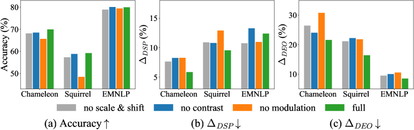
Figure 2: Ablation study on the effect of each module.

5 Related Work

We only present the most related work here, while leaving the rest to Appendix H due to space limitation.

Fairness learning. Fairness learning (Zemel et al. 2013; Kusner et al. 2017) can be broadly categorized into three kinds. (1) Pre-processing methods usually eliminate bias by reshaping the dataset (Feldman et al. 2015), such as correcting the labels (Kamiran and Calders 2009). (2) In-processing methods usually rely on model refinement for debiasing, such as applying additional regularizations or constraints (Dwork et al. 2012; Zafar et al. 2017). (3) Post-processing methods (Hardt, Price, and Srebro 2016; Pleiss et al. 2017) usually designate new labels on the predictions to remove bias.

Some recent approaches (Rahman et al. 2019; Bose and Hamilton 2019; Dai and Wang 2021; Wang et al. 2022) deal with the sensitive attribute-based fairness on graphs. FairWalk (Rahman et al. 2019) tries to sample fair paths by guiding random walks based on sensitive attributes, while FairAdj (Li et al. 2021) studies dyadic fairness for link prediction by adjusting the adjacency matrix. On the other hand, EDITS (Dong et al. 2022) proposes to debias the input attributed data so that GNNs can be fed with less biased data, while FairVGNN (Wang et al. 2022) tries to address the issue of sensitive attribute leakage by automatically identifying and masking correlated attributes. Others (Bose and Hamilton 2019; Dai and Wang 2021; Feng et al. 2019) employ discriminators (Goodfellow et al. 2014) as additional constraints on the encoder to facilitate the identification of sensitive attributes. DeBayes (Buyl and De Bie 2020) trains a conditional network embedding (Kang, Lijffijt, and De Bie 2019) by using a biased prior and evaluates the model with an oblivious prior, thus reducing the impact of sensitive attributes. Ma et al. (Ma, Deng, and Mei 2021) investigate the performance disparity between test groups rooted in the distance between them and the training instances. Dong et al. (Dong et al. 2021) study the individual fairness for GNNs from the ranking perspective. Besides, there are fairness learning studies on heterogeneous (Zeng et al. 2021) and knowledge graphs (Fisher et al. 2020). However, none of these works is designed for degree fairness on graphs.

Degree-specific GNNs. Some recent studies investigate the influence of degrees on the performance of GNNs. Various strategies have been proposed, such as employing degree-specific transformations on nodes (Wu, He, and Xu 2019; Tang et al. 2020), accounting for their different roles (Ahmed et al. 2020), balancing the sampling of nodes in random walks (Kojaku et al. 2021), or considering the degree-related performance differences between nodes (Kang et al. 2022; Liu et al. 2020; Liu, Nguyen, and Fang 2021). However, they emphasize the structural difference between nodes in order to improve task accuracy, rather than to eliminate the degree bias for fairness.

6 Conclusions

In this paper, we investigated the important problem of degree fairness on GNNs. In particular, we made the first attempt on defining and addressing the generalized degree fairness issue. To eliminate the degree bias rooted in the layer-wise neighborhood aggregation, we proposed a novel generalized degree fairness-centric GNN framework named DegFairGNN, which can flexibly work with most modern GNNs. The key insight is to target the root of degree bias, by modulating the core operation of neighborhood aggregation through a structural contrast. We conducted extensive experiments on three benchmark datasets and achieved promising results on both accuracy and fairness metrics.

7 Acknowledgments

This research is supported by the Agency for Science, Technology and Research (A*STAR) under its AME Programmatic Funds (Grant No. A20H6b0151).

References

- Agarwal, Lakkaraju, and Zitnik (2021) Agarwal, C.; Lakkaraju, H.; and Zitnik, M. 2021. Towards a unified framework for fair and stable graph representation learning. In Uncertainty in Artificial Intelligence, 2114–2124. PMLR.
- Ahmed et al. (2020) Ahmed, N.; Rossi, R. A.; Lee, J.; Willke, T.; Zhou, R.; Kong, X.; and Eldardiry, H. 2020. Role-based graph embeddings. IEEE Transactions on Knowledge and Data Engineering.
- Bose and Hamilton (2019) Bose, A.; and Hamilton, W. 2019. Compositional fairness constraints for graph embeddings. In International Conference on Machine Learning, 715–724. PMLR.
- Buyl and De Bie (2020) Buyl, M.; and De Bie, T. 2020. DeBayes: a Bayesian method for debiasing network embeddings. In International Conference on Machine Learning, 1220–1229. PMLR.
- Dai and Wang (2021) Dai, E.; and Wang, S. 2021. Say No to the Discrimination: Learning Fair Graph Neural Networks with Limited Sensitive Attribute Information. In Proceedings of the 14th ACM International Conference on Web Search and Data Mining, 680–688.
- Dong et al. (2021) Dong, Y.; Kang, J.; Tong, H.; and Li, J. 2021. Individual fairness for graph neural networks: A ranking based approach. In Proceedings of the 27th ACM SIGKDD Conference on Knowledge Discovery & Data Mining, 300–310.
- Dong et al. (2022) Dong, Y.; Liu, N.; Jalaian, B.; and Li, J. 2022. Edits: Modeling and mitigating data bias for graph neural networks. In Proceedings of the ACM Web Conference 2022, 1259–1269.
- Dwork et al. (2012) Dwork, C.; Hardt, M.; Pitassi, T.; Reingold, O.; and Zemel, R. 2012. Fairness through awareness. In Proceedings of the 3rd innovations in theoretical computer science conference, 214–226.
- Feldman et al. (2015) Feldman, M.; Friedler, S. A.; Moeller, J.; Scheidegger, C.; and Venkatasubramanian, S. 2015. Certifying and removing disparate impact. In proceedings of the 21th ACM SIGKDD international conference on knowledge discovery and data mining, 259–268.
- Feng et al. (2019) Feng, R.; Yang, Y.; Lyu, Y.; Tan, C.; Sun, Y.; and Wang, C. 2019. Learning fair representations via an adversarial framework. arXiv preprint arXiv:1904.13341.
- Fisher et al. (2020) Fisher, J.; Mittal, A.; Palfrey, D.; and Christodoulopoulos, C. 2020. Debiasing knowledge graph embeddings. In Proceedings of the 2020 Conference on Empirical Methods in Natural Language Processing (EMNLP), 7332–7345.
- Goodfellow et al. (2014) Goodfellow, I.; Pouget-Abadie, J.; Mirza, M.; Xu, B.; Warde-Farley, D.; Ozair, S.; Courville, A.; and Bengio, Y. 2014. Generative adversarial nets. In NeurIPS, 2672–2680.
- Ha, Dai, and Le (2017) Ha, D.; Dai, A.; and Le, Q. V. 2017. Hypernetworks. In ICLR.
- Hamilton, Ying, and Leskovec (2017) Hamilton, W.; Ying, Z.; and Leskovec, J. 2017. Inductive representation learning on large graphs. In Advances in neural information processing systems, 1024–1034.
- Hardt, Price, and Srebro (2016) Hardt, M.; Price, E.; and Srebro, N. 2016. Equality of Opportunity in Supervised Learning. Advances in Neural Information Processing Systems, 29: 3315–3323.
- Kamiran and Calders (2009) Kamiran, F.; and Calders, T. 2009. Classifying without discriminating. In 2009 2nd International Conference on Computer, Control and Communication, 1–6. IEEE.
- Kang, Lijffijt, and De Bie (2019) Kang, B.; Lijffijt, J.; and De Bie, T. 2019. Conditional network embeddings. In International Conference on Learning Representations.
- Kang et al. (2022) Kang, J.; Zhu, Y.; Xia, Y.; Luo, J.; and Tong, H. 2022. Rawlsgcn: Towards rawlsian difference principle on graph convolutional network. In Proceedings of the ACM Web Conference 2022, 1214–1225.
- Kipf and Welling (2017) Kipf, T. N.; and Welling, M. 2017. Semi-supervised classification with graph convolutional networks. ICLR.
- Kojaku et al. (2021) Kojaku, S.; Yoon, J.; Constantino, I.; and Ahn, Y.-Y. 2021. Residual2Vec: Debiasing graph embedding with random graphs. In NeurIPS.
- Kusner et al. (2017) Kusner, M.; Loftus, J.; Russell, C.; and Silva, R. 2017. Counterfactual Fairness. Advances in Neural Information Processing Systems 30 (NIPS 2017), 30.
- Li et al. (2021) Li, P.; Wang, Y.; Zhao, H.; Hong, P.; and Liu, H. 2021. On dyadic fairness: Exploring and mitigating bias in graph connections. In International Conference on Learning Representations.
- Liu et al. (2021) Liu, Z.; Fang, Y.; Liu, C.; and Hoi, S. C. 2021. Node-wise Localization of Graph Neural Networks. In Proceedings of the Thirtieth International Joint Conference on Artificial Intelligence, 1520–1526.
- Liu, Nguyen, and Fang (2021) Liu, Z.; Nguyen, T.-K.; and Fang, Y. 2021. Tail-GNN: Tail-Node Graph Neural Networks. In Proceedings of the 27th ACM SIGKDD Conference on Knowledge Discovery & Data Mining, 1109–1119.
- Liu et al. (2020) Liu, Z.; Zhang, W.; Fang, Y.; Zhang, X.; and Hoi, S. C. 2020. Towards locality-aware meta-learning of tail node embeddings on networks. In Proceedings of the 29th ACM International Conference on Information & Knowledge Management, 975–984.
- Ma et al. (2021) Ma, J.; Chang, B.; Zhang, X.; and Mei, Q. 2021. CopulaGNN: Towards Integrating Representational and Correlational Roles of Graphs in Graph Neural Networks. In International Conference on Learning Representations.
- Ma, Deng, and Mei (2021) Ma, J.; Deng, J.; and Mei, Q. 2021. Subgroup generalization and fairness of graph neural networks. In NeurIPS.
- Newman (2005) Newman, M. E. 2005. Power laws, Pareto distributions and Zipf’s law. Contemporary physics, 46(5): 323–351.
- Pedreshi, Ruggieri, and Turini (2008) Pedreshi, D.; Ruggieri, S.; and Turini, F. 2008. Discrimination-aware data mining. In Proceedings of the 14th ACM SIGKDD international conference on Knowledge discovery and data mining, 560–568.
- Pei et al. (2020) Pei, H.; Wei, B.; Chang, K. C.-C.; Lei, Y.; and Yang, B. 2020. Geom-GCN: Geometric Graph Convolutional Networks. In International Conference on Learning Representations.
- Perez et al. (2018) Perez, E.; Strub, F.; De Vries, H.; Dumoulin, V.; and Courville, A. 2018. Film: Visual reasoning with a general conditioning layer. In Thirty-Second AAAI Conference on Artificial Intelligence.
- Pleiss et al. (2017) Pleiss, G.; Raghavan, M.; Wu, F.; Kleinberg, J.; and Weinberger, K. Q. 2017. On Fairness and Calibration. Advances in Neural Information Processing Systems, 30: 5680–5689.
- Rahman et al. (2019) Rahman, T. A.; Surma, B.; Backes, M.; and Zhang, Y. 2019. Fairwalk: Towards Fair Graph Embedding. In IJCAI, 3289–3295.
- Tang et al. (2020) Tang, X.; Yao, H.; Sun, Y.; Wang, Y.; Tang, J.; Aggarwal, C.; Mitra, P.; and Wang, S. 2020. Investigating and Mitigating Degree-Related Biases in Graph Convoltuional Networks. In Proceedings of the 29th ACM International Conference on Information & Knowledge Management, 1435–1444.
- Vaswani et al. (2017) Vaswani, A.; Shazeer, N.; Parmar, N.; Uszkoreit, J.; Jones, L.; Gomez, A. N.; Kaiser, Ł.; and Polosukhin, I. 2017. Attention is All you Need. Advances in Neural Information Processing Systems, 30: 5998–6008.
- Veličković et al. (2018) Veličković, P.; Cucurull, G.; Casanova, A.; Romero, A.; Lio, P.; and Bengio, Y. 2018. Graph attention networks. ICLR.
- Wang et al. (2022) Wang, Y.; Zhao, Y.; Dong, Y.; Chen, H.; Li, J.; and Derr, T. 2022. Improving Fairness in Graph Neural Networks via Mitigating Sensitive Attribute Leakage. In SIGKDD.
- Wu, He, and Xu (2019) Wu, J.; He, J.; and Xu, J. 2019. Demo-Net: Degree-specific graph neural networks for node and graph classification. In Proceedings of the 25th ACM SIGKDD International Conference on Knowledge Discovery & Data Mining, 406–415.
- Xu et al. (2018) Xu, K.; Li, C.; Tian, Y.; Sonobe, T.; Kawarabayashi, K.-i.; and Jegelka, S. 2018. Representation Learning on Graphs with Jumping Knowledge Networks. In ICML, 5453–5462.
- Zafar et al. (2017) Zafar, M. B.; Valera, I.; Rogriguez, M. G.; and Gummadi, K. P. 2017. Fairness constraints: Mechanisms for fair classification. In Artificial Intelligence and Statistics, 962–970. PMLR.
- Zemel et al. (2013) Zemel, R.; Wu, Y.; Swersky, K.; Pitassi, T.; and Dwork, C. 2013. Learning fair representations. In International conference on machine learning, 325–333. PMLR.
- Zeng et al. (2021) Zeng, Z.; Islam, R.; Keya, K. N.; Foulds, J.; Song, Y.; and Pan, S. 2021. Fair Representation Learning for Heterogeneous Information Networks. arXiv preprint arXiv:2104.08769.