A Generalized Surface Loss for Reducing the Hausdorff Distance in Medical Imaging Segmentation

Abstract

Within medical imaging segmentation, the Dice coefficient and Hausdorff-based metrics are standard measures of success for deep learning models. However, modern loss functions for medical image segmentation often only consider the Dice coefficient or similar region-based metrics during training. As a result, segmentation architectures trained over such loss functions run the risk of achieving high accuracy for the Dice coefficient but low accuracy for Hausdorff-based metrics. Low accuracy on Hausdorff-based metrics can be problematic for applications such as tumor segmentation, where such benchmarks are crucial. For example, high Dice scores accompanied by significant Hausdorff errors could indicate that the predictions fail to detect small tumors. We propose the Generalized Surface Loss function, a novel loss function to minimize Hausdorff-based metrics with more desirable numerical properties than current methods and with weighting terms for class imbalance. Our loss function outperforms other losses when tested on the LiTS and BraTS datasets using the state-of-the-art nnUNet architecture. These results suggest we can improve medical imaging segmentation accuracy with our novel loss function.

1 Introduction

Deep learning has become a popular framework in medical image analysis, automating and standardizing essential tasks such as segmenting regions of interest. This process is crucial for computer-assisted diagnosis, intervention, and therapy [39]. Despite its importance, manual image segmentation can be a tedious and time-consuming task with variable results among users [45, 18]. Fully automated segmentation offers a solution, reducing time and producing more consistent results [45, 18]. Convolutional neural networks (CNNs) have achieved notable success in segmentation tasks, including labeling tumors and anatomical structures [37, 13, 20].

In medical imaging segmentation, the performance of automatic methods is usually evaluated using common metrics like the Dice similarity coefficient, average surface distance (ASD), and the Hausdorff distance (HD) [15, 44]. The HD is beneficial among these metrics because it indicates the largest segmentation error. As sketched out in Figure 1, for two sets of points $X$ and $Y$, the one-sided HD from $X$ to $Y$ is given by

$$\text{hd}(X,Y)=\max_{x\in X}\min_{y\in Y}||x-y||_{2}.$$ (1)

The one-sided HD is not a true distance metric since it is not commutative (i.e., $\text{hd}(X,Y)\neq\text{hd}(Y,X)$). To address this, we consider the bidirectional or total Hausdorff distance, which is given by

$$\text{HD}(X,Y)=\max\{\text{hd}(X,Y),\text{hd}(Y,X)\}.$$ (2)

In (2), we use the Euclidean distance, but any other distance metric can be used. Intuitively, the HD is the longest distance from one point in a set to the closest point in the other.

Although the HD and other similar metrics like the ASD are widely used for evaluating medical imaging segmentation models, many current loss functions for medical image segmentation only consider the Dice coefficient or similar region-based metrics during training [22, 38, 1, 41, 8]. This approach runs the risk of achieving high accuracy for the Dice coefficient but low accuracy for Hausdorff-based metrics [24, 23, 44]. This low accuracy is particularly problematic for applications such as tumor segmentation, where Hausdorff-based metrics are crucial for evaluating segmentation accuracy [35]. For example, high Dice scores accompanied by significant Hausdorff errors could indicate that the predictions fail to detect small tumors. As a result, we propose the Generalized Surface Loss function, a novel loss function to minimize the Hausdorff distance (HD). This loss function incorporates a normalization scheme to give it more desirable numerical properties than current methods and uses weighting terms to address class imbalance.

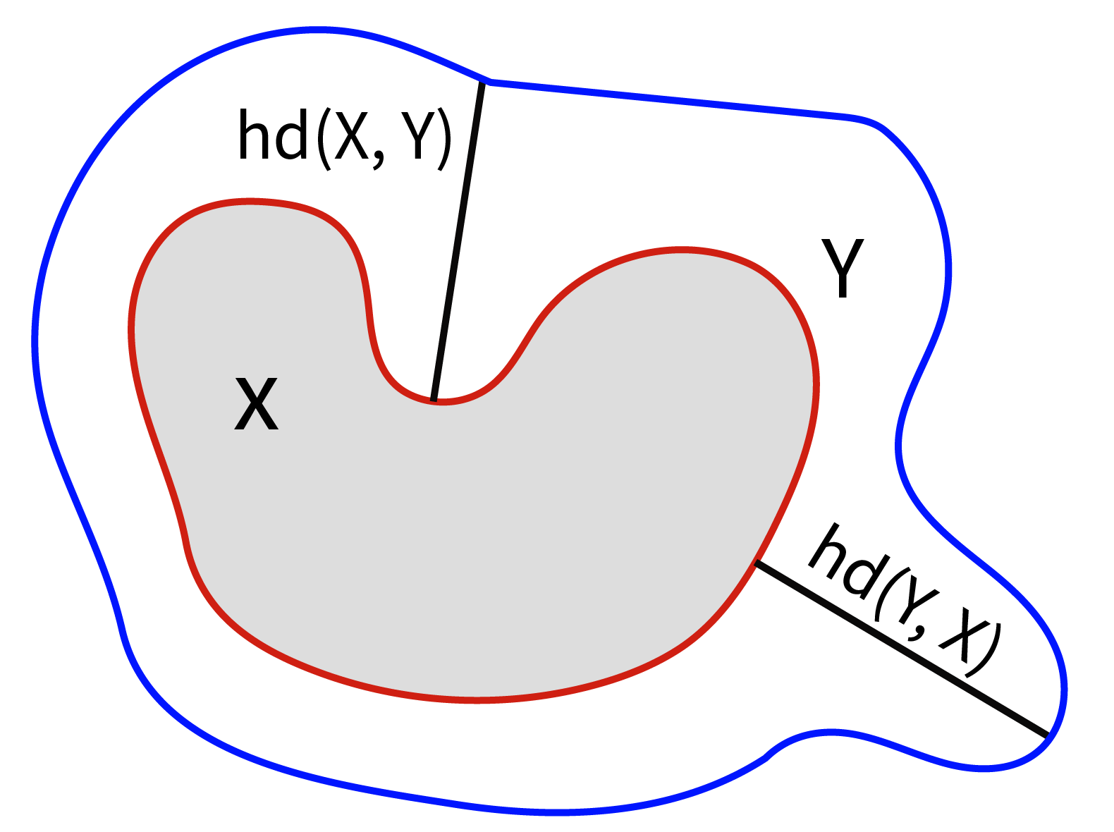
Figure 1: Illustration of the Hausdorff distance between two sets of points $X$ and $Y$.

1.1 Previous Work

Over the last several years, multiple loss functions have been developed for medical image segmentation models. Broadly, these loss functions fall into two categories: region and boundary-based loss functions. We briefly survey these loss functions below.

1.1.1 Region-Based Losses

Dice Loss

- The Dice coefficient is a widely used metric in computer vision tasks to calculate the global measure of overlap between two binary sets [16]. Introduced by Milletari et al. [34], the Dice Loss (DL) function directly incorporates this metric into the formulation as follows:

$$\mathcal{L}_{dice}=1-\frac{1}{C}\sum_{k=1}^{C}\frac{2\sum_{i=1}^{N}T_{i}^{k}P_{i}^{k}}{\sum_{i=1}^{N}\left(T_{i}^{k}\right)^{2}+\sum_{i=1}^{N}\left(P_{i}^{k}\right)^{2}},$$ (3)

where $N$ denotes the total number of pixels (or voxels in the 3D case), $C$ denotes the number of segmentation classes, $P_{i}^{k}\in[0,1]$ is the $i$-th voxel in the $k$-th class of the predicted segmentation mask, and $T_{i}^{k}\in\{0,1\}$ is the same for the ground truth. It is also common for the DL to be used in conjunction with the cross entropy loss function [20, 22, 48, 43]. This composite loss (which we call the Dice-CE loss) adds a cross-entropy term to (3) and is given by

$$\mathcal{L}_{dice-ce}=\mathcal{L}_{dice}-\frac{1}{CN}\sum_{k=1}^{C}\sum_{i=1}^{N}T_{i}^{k}\log\left(P_{i}^{k}\right)$$ (4)

The use of DL (and Dice-CE loss) in the training of deep learning models for medical imaging segmentation tasks is widespread [20, 22, 2, 29, 49, 8]. This is because the Dice coefficient is a widely recognized metric for measuring the global overlap between the predicted and ground truth segmentation masks. However, the DL is a region-based loss that does not take into account the HD during training. As a result, models trained using the DL function can achieve high accuracy with respect to the Dice coefficient, but exhibit poor accuracy with respect to HD-based metrics [4]. This low accuracy is particularly problematic for tasks such as tumor segmentation, where HD-based metrics are crucial to evaluate the accuracy of segmentation [35].

Generalized Dice Loss

- Sudre et al. proposed the Generalized Dice Loss (GDL) [41] by introducing a weighting term to the DL function presented above. In their work, the addition of these weight terms produced better Dice scores for highly imbalanced segmentation problems. The GDL loss is given by the following:

$$\mathcal{L}_{gdl}=1-2\frac{\sum_{k=1}^{C}w_{k}\sum_{i=1}^{N}T_{i}^{k}P_{i}^{k}}{\sum_{k=1}^{C}w_{k}\sum_{i=1}^{N}\left(\left(T_{i}^{k}\right)^{2}+\left(P_{i}^{k}\right)^{2}\right)},$$ (5)

where the term $w_{k}$ is the weighting term for the $k$-th class and is given by

$$w_{k}=\frac{1}{\left(\sum_{i=1}^{N}T_{i}^{k}\right)^{2}}.$$ (6)

The intuition behind $w_{k}$ is that the contribution of each labeled class is the inverse of its area (or volume in the 3D case). Hence, this weighting can help reduce the well-known correlation between region size and the Dice score [41, 27, 46]. However, like the DL, the GDL is a region-based loss and does not consider the HD, and can result in poor accuracy for HD-based metrics. Additionally, the weights $w_{k}$ change for each training example, which makes the optimization process more challenging, as the problem is altered for every batch.

1.1.2 Boundary-Based Losses

Hausdorff Loss

- Karimi et al. introduced a Hausdorff Loss (HL) that incorporates an estimation of the HD in the loss function via Distance Transform Maps (DTM) [24]. A DTM represents the distance between each voxel and the closest boundary or edge of an object. The values in a DTM are positive on the exterior, zero on the boundary, or negative in the interior of the object. Figure 2 illustrates an example segmentation image and its corresponding DTM.

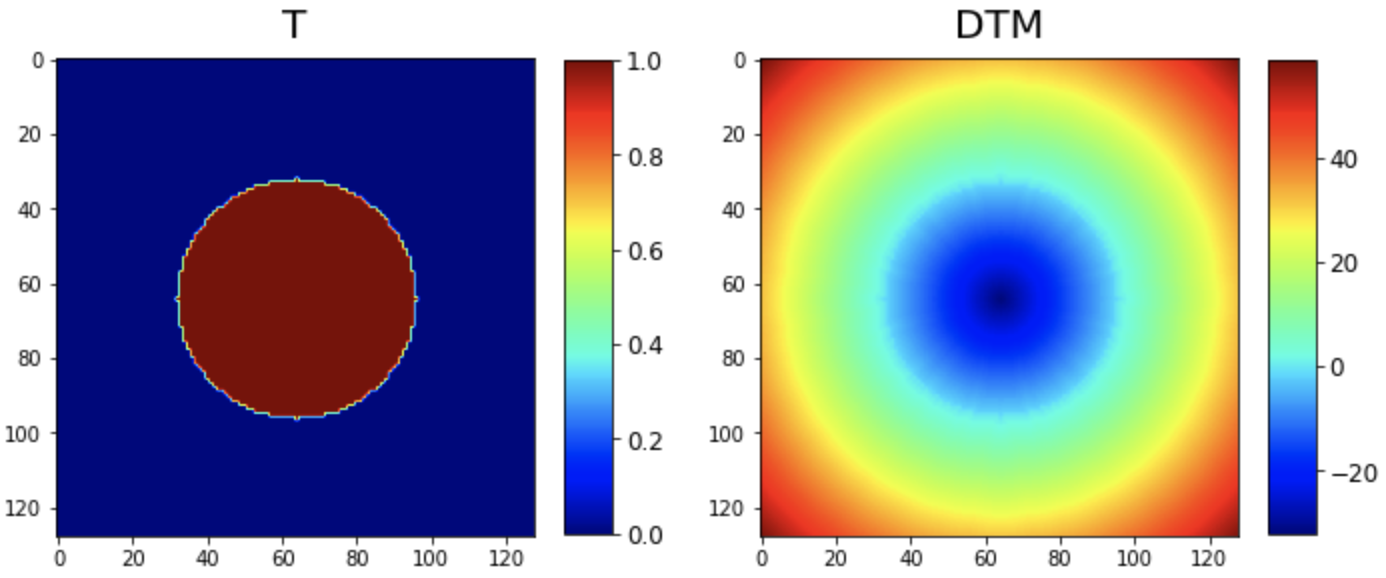
Figure 2: (Left) Example segmentation. (Right) DTM for example segmentation. Here, the values in the DTM are positive on the exterior, zero on the boundary, or negative in the object’s interior.

The HL is given by the following:

$$\mathcal{L}_{haus}=\frac{1}{CN}\sum_{k=1}^{C}\sum_{i=1}^{N}(T_{i}^{k}-P_{i}^{k})^{2}\left(\left(D_{i}^{k}\right)^{2}+\left(\bar{D}_{i}^{k}\right)^{2}\right),$$ (7)

where $D_{i}^{k}$ is the $i$-th voxel in the DTM for the $k$-th class in the ground truth, and where $\bar{D}_{i}^{k}$ is the same for the prediction. This function is used in a weighted combination with a region-based loss $\mathcal{L}_{region}$ so that the overall loss function is given by

$$\mathcal{L}=\alpha\mathcal{L}_{region}+(1-\alpha)\mathcal{L}_{haus}$$ (8)

where the scalar $\alpha=1$ in the first epoch and decreases linearly until $\alpha=0$. While the HL does consider the HD, it requires the re-computation of the DTM for each predicted segmentation at each epoch. It also requires the storage of the whole volume in memory since one cannot compute the DTM for a subset of the volume. Although the DTM can be computed in linear time [31], reconstructing the DTM of the whole volume for each training batch results in a significant slowdown in training [23]. These two factors make the HL computationally expensive and difficult to incorporate into current patch-based medical imaging segmentation pipelines like nnUNet, MONAI, or MIST [20, 11, 12]. To address these issues, Karimi et al. introduce a one-sided version of (7), which does not consider the DTM of the prediction. The HL will refer to this one-sided version for the remainder of this work.

Boundary Loss

- Kervadec et al. proposed a Boundary Loss (BL) function, which considers the measure of distance to the boundary of a region [24]. Like the HL function, the BL uses a DTM to measure the distance to the boundary of the ground truth image. The BL loss is given by the following:

$$\mathcal{L}_{bl}=\frac{1}{CN}\sum_{k=1}^{C}\sum_{i=1}^{N}D_{i}^{k}P_{i}^{k}.$$ (9)

Also like the HL, the BL uses a weighted combination with a region-based loss so that the overall loss is given by an expression similar to (8), but with $\mathcal{L}_{bl}$. Again, $\alpha=1$ at the start of training and decreases linearly until $\alpha=0$ in the final epoch.

Intuitively, the BL function measures the average distance of each voxel in the predicted segmentation mask to the boundary of the ground truth mask. Unlike the HL, the BL does not require the re-computation of DTMs at each epoch, making it comparatively inexpensive from a computational point of view. However, region-based loss functions such as DL and GDL are bounded, achieving values in the interval [0,1]. On the other hand, the BL function is unbounded since $D_{i}^{k}\in(-\infty,\infty)$. This unboundedness can result in large positive or negative loss values and minimums that depend on individual image sizes and voxel spacings, making optimization more difficult. This same issue can also dominate the total loss, causing the contribution of the region-based loss to become negligible during training.

2 Materials and Methods

2.1 Generalized Surface Loss

We seek a boundary-based loss function that is 1) bounded in the interval $[0,1]$ to ensure that its contribution to the overall loss function does not dominate the region-based loss in (8), 2) is computationally tractable like the BL, and 3) is weighted by pre-computed weighting terms to handle class imbalance while not changing the optimization problem for each batch like the GDL. Now, consider a “worst” case prediction $\mathbf{1}-T$, which maximizes the value

$$\sum_{i=1}^{N}\left(D_{i}\left(\left(1-T_{i}\right)-T_{i}\right)\right)^{2}.$$ (10)

Note that a worst case is dependent on the choice of metric, but for our purposes we choose to maximize (10) so that for a given prediction $P$, we have

$$0\leq\frac{\sum_{i=1}^{N}\left(D_{i}\left((1-T_{i})-P_{i}\right)\right)^{2}}{\sum_{i=1}^{N}\left(D_{i}\left((1-T_{i})-T_{i}\right)\right)^{2}}\leq 1.$$ (11)

Simplifying, adding weighting terms for class imbalance, and subtracting the final value from one gives us the Generalized Surface Loss (GSL):

$$\mathcal{L}_{gsl}=1-\frac{\sum_{k=1}^{C}w_{k}\sum_{i=1}^{N}\left(D_{i}^{k}\left(1-\left(T_{i}^{k}+P_{i}^{k}\right)\right)\right)^{2}}{\sum_{k=1}^{C}w_{k}\sum_{i=1}^{N}\left(D_{i}^{k}\right)^{2}}.$$ (12)

We pre-compute the class weights $w_{k}$ so that the inverse of the total number of voxels belonging to each class over the entire dataset $N_{k}$ is normalized by the sum of the other inverses. For the $k$-th segmentation class, $w_{k}$ is given by

$$w_{k}=\left(\frac{1}{\sum_{j=1}^{C}\frac{1}{N_{j}}}\right)\frac{1}{N_{k}}.$$ (13)

Like BL and HL, the overall loss function uses a scheme similar to (8). However, in addition to a linear schedule, we also propose the use of the step and cosine functions as schedules for setting $\alpha$ at each epoch. In each case, we decrease until $\alpha=0$ in the final epoch. To define each schedule, let $h\geq 1$ be our step length, $t$ be the current epoch, and $T$ be the total number of epochs. Then define $N_{h}=\lfloor T/h\rfloor$. The value of $\alpha$ at $t$ for each schedule is given by

$$\alpha_{linear}(t) =1-\frac{t}{T}$$ (14)

$$\alpha_{step}(t) =1-\frac{\lfloor t/h\rfloor}{N_{h}}$$ (15)

$$\alpha_{cosine}(t) =\frac{1}{2}\left(1+\cos{\frac{\pi t}{T}}\right)$$ (16)

2.2 Network Architecture

We examine the effects of our proposed loss function on the widely used nnUNet architecture [20]. The nnUNet architecture uses an adaptive framework based on the properties of the given dataset (i.e., patch size and voxel spacing) to build a U-shaped architecture like the 3D U-Net [37, 13]. As a result, the network has achieved state-of-the-art accuracy on several recent public medical imaging segmentation challenges [21, 3, 19]. In the context of our work, the nnUNet architecture provides a state-of-the-art baseline for our analysis.

2.3 Data

We test our proposed loss function on the MICCAI Liver and Tumor Segmentation (LiTS) Challenge 2017 dataset [9] and the multi-label tumor segmentation in the MICCAI Brain Tumor Segmentation (BraTS) Challenge 2020 dataset [33, 6, 5]. In the context of our work, these datasets allow us to test each loss function on two different imaging modalities (i.e., CT and MR) and have non-trivial preprocessing and segmentation tasks. We briefly describe these datasets and the preprocessing steps we take below.

For the LiTS dataset, we perform binary liver segmentation. This dataset consists of the 131 CT scans from the MICCAI 2017 Challenge’s multi-institutional training set. These scans vary significantly in the number of slices in the axial direction and voxel resolution, although all axial slices are at 512$\times$512 resolution. As a result, we use the preprocessing steps proposed by [20] to handle this variability. Namely, we resample each image to the median resolution of the training data in the $x$ and $y$-directions and use the 90th percentile resolution in the $z$-direction. For intensity normalization, we window each image according to the foreground voxels’ 0.5 and 99.5 percentile intensity values across all of the training data. This scheme results in windowing from -17 to 201 HU. We also apply z-score normalization according to the foreground voxels’ mean and standard deviation. The LiTS dataset is available for download https://competitions.codalab.org/competitions/17094#learn_the_details-overview.

The BraTS training set contains 369 multimodal scans from 19 institutions. Each set of scans includes a T1-weighted, post-contrast T1-weighted, T2-weighted, and T2 Fluid Attenuated Inversion Recovery volume along with a multi-label ground truth segmentation. The annotations include the GD-enhancing tumor (ET - label 4), the peritumoral edema (ED - label 2), and the necrotic and non-enhancing tumor core (NCR/NET - label 1). The final segmentation classes are the whole tumor (WT - labels 1, 2, and 4), tumor core (TC - labels 2 and 4), and ET. All volumes are provided at an isotropic voxel resolution of 1$\times$1$\times$1 $\text{mm}^{3}$, co-registered to one another, and skull stripped, with a size of 240$\times$240$\times$155. We crop each image according to the brainmask (i.e., non-zero voxels) and apply z-score intensity normalization on only non-zero voxels for preprocessing. The BraTS training dataset is available for download at https://www.med.upenn.edu/cbica/brats2020/registration.html.

2.4 Training and Testing

We compare the effect on segmentation performance for each loss function described in Section 1.1 and 2. We select $\mathcal{L}_{region}$ for our boundary-based loss functions to be the Dice-CE loss. We use the Adam optimizer with the learning rate set to 0.0003. A five-fold cross-validation scheme is used to train and evaluate each loss function. During training, we select a batch size of two, using a patch size of 128$\times$128$\times$128 for the BraTS dataset and 256$\times$256$\times$128 for the LiTS dataset. We apply the same random augmentation described in [20]. Our models are implemented in Python using PyTorch (v2.0.1) and trained on two NVIDIA Quadro RTX 8000 GPUs using the DistributedDataParallel module [36, 25]. All network weights are initialized using the default PyTorch initializers. For reproducibility, we set all random seeds to 42. All other hyperparameters are left at their default values. The code for this work is available at https://anonymous.4open.science/r/gen-surf-loss-B624/README.md.

We used three common medical imaging segmentation metrics to evaluate the accuracy of our predictions - the Dice coefficient, 95th percentile Hausdorff distance, and average surface distance (ASD). These metrics are implemented using the SimpleITK Python package [28, 47, 7]. We briefly describe these metrics below.

Dice Coefficient - As described in the Dice loss function description, the Dice coefficient is a widely used measure of overlap in computer vision tasks. More specifically, it measures the overlap between the two binary sets. It ranges from 0 to 1, where 1 indicates a perfect match between the predicted and ground truth segmentations.

95th Percentile Hausdorff Distance - While the Dice score is a commonly used metric for comparing two segmentation masks, it is not sensitive to local differences, as it represents a global measure of overlap. Therefore, we compute a complementary metric, the 95th percentile Hausdorff distance (HD95), which is a distance metric that measures the maximum of the minimum distances between the predicted segmentation and the ground truth at the 95th percentile. The HD95 is a non-negative real number measured in millimeters, with a value of 0mm indicating a perfect prediction.

Average Surface Distance - The average surface distance (ASD) measures the average distance between the predicted segmentation and the ground truth along the surface of the object being segmented. It is a more fine-grained metric than the HD95 since it captures the surface-level details of the segmentation and can provide insight into the quality of the segmentation. The ASD is a non-negative real number measured in millimeters with a perfect prediction achieving a value of 0mm.

3 Results

Using the methods described in Section 2, we train a nnUNet using each loss function described in Section 1.1 and compare their performance to our proposed GSL function. This experiment uses a linear schedule for the parameter $\alpha$ in the boundary-based losses (i.e., HL, BL, and GSL). Table 1 shows the results of this comparison. Here, our GSL achieves lower Hausdorff 95 and average surface distances for the LiTS and BraTS challenge datasets. Figures 3 and 4 show from left to right the ground truth and predictions from the nnUNet architecture trained on LiTS and BraTS data respectively, with the Dice-CE, BL, and GSL functions for a spectrum of easier to more difficult test cases. Even for more difficult cases, we see that the GSL produces visually superior predictions than the Dice-CE and BL functions.

Dataset	Task	Loss	Dice [$\uparrow$]	Hausdorf 95 (mm) [$\downarrow$]	Avg. Surface (mm) [$\downarrow$]
LiTS	Liver	DL	0.9304 (0.0974)	9.0655 (30.530)	3.7608 (11.976)
		Dice-CE	0.9287 (0.1229)	10.874 (35.205)	3.7455 (11.361)
		GDL	0.9246 (0.1317)	9.0825 (28.023)	3.6259 (10.693)
		HL	0.9166 (0.1237)	17.451 (71.162)	9.5963 (64.328)
		BL	0.9270 (0.1221)	12.366 (66.451)	7.9931 (63.268)
		GSL	0.9302 (0.1075)	8.9046 (28.205)	3.2791 (7.0823)
BraTS	Whole Tumor	DL	0.9027 (0.0784)	3.9117 (10.236)	1.2931 (2.0569)
		Dice-CE	0.9048 (0.0771)	4.2284 (12.342)	1.2852 (2.0275)
		GDL	0.8508 (0.1303)	7.6853 (16.766)	2.3204 (3.5123)
		HL	0.8607 (0.1117)	5.0997 (10.997)	1.7400 (2.2935)
		BL	0.9011 (0.0740)	3.9045 (10.036)	1.2400 (1.7657)
		GSL	0.9087 (0.0722)	3.5367 (9.7121)	1.1442 (1.8159)
	Tumor Core	DL	0.8403 (0.1803)	5.5020 (12.859)	1.7861 (3.7423)
		Dice-CE	0.8413 (0.1742)	5.8953 (15.191)	1.7464 (3.1522)
		GDL	0.7799 (0.2640)	7.7837 (16.793)	2.6613 (5.1596)
		HL	0.7519 (0.2102)	7.8241 (21.669)	3.5736 (19.697)
		BL	0.8318 (0.1781)	5.4368 (12.532)	1.7446 (3.2988)
		GSL	0.8448 (0.1835)	4.9526 (11.333)	1.8121 (4.9699)
	Enhancing Tumor	DL	0.7422 (0.2791)	32.704 (96.645)	28.640 (96.886)
		Dice-CE	0.7424 (0.2773)	32.593 (96.689)	28.539 (96.878)
		GDL	0.7431 (0.2738)	32.369 (95.088)	27.792 (95.176)
		HL	0.6831 (0.2773)	32.196 (94.416)	27.833 (95.141)
		BL	0.7395 (0.2770)	30.971 (94.723)	27.520 (95.218)
		GSL	0.7587 (0.2696)	30.121 (93.228)	26.551 (93.568)

Table 1: Mean and standard deviation of each metric for each loss function using the nnUNet architecture. Here, we see that our GSL achieves lower Hausdorff 95 and average surface distances for the LiTS and BraTS challenge datasets.

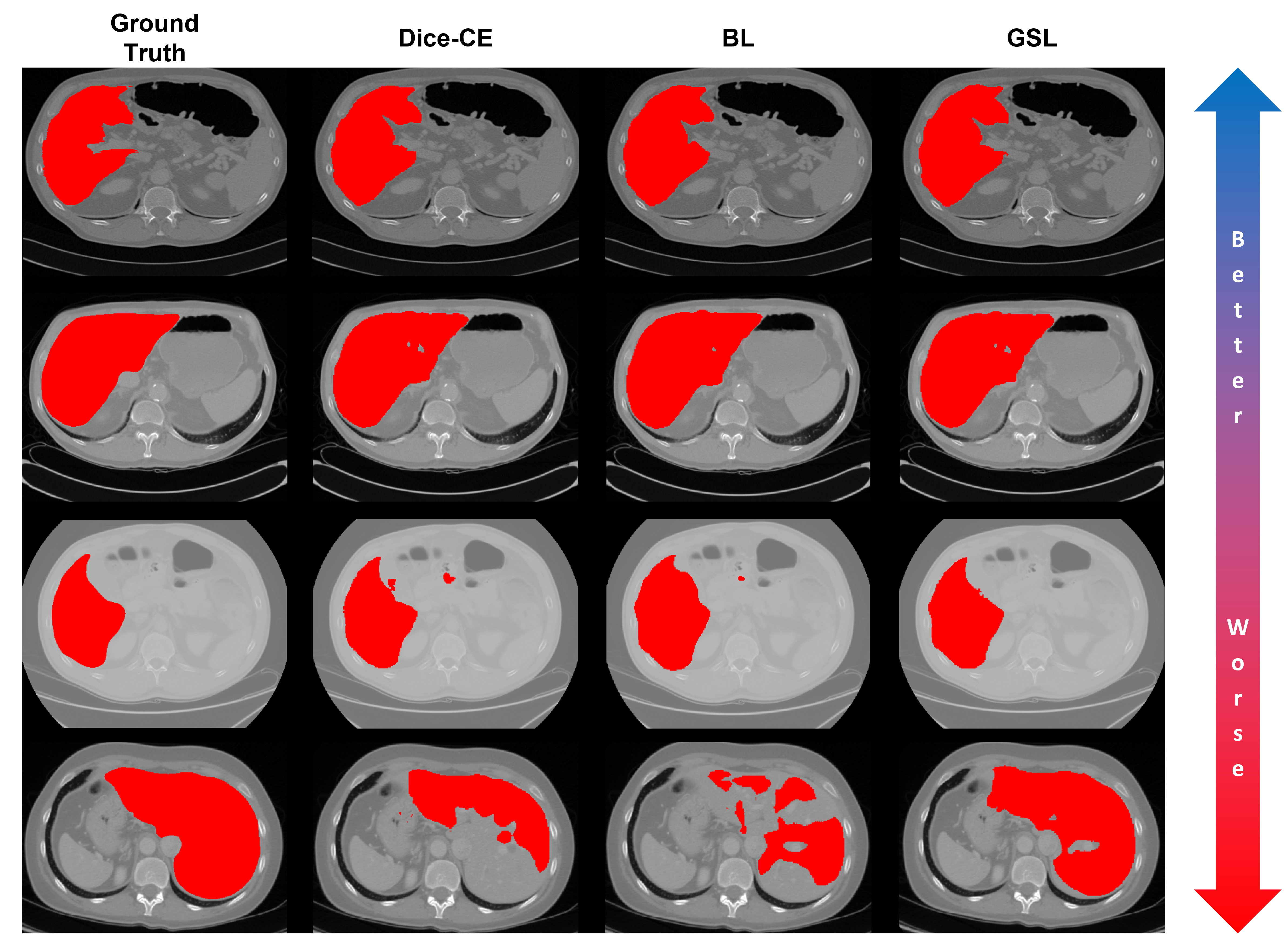
Figure 3: From left to right, ground truth and predictions from the nnUNet architecture trained on LiTS data with Dice-CE, BL, and GSL functions for a spectrum of easier to more difficult test cases. Here, we see that, even for more difficult cases, the GSL produces visually superior predictions than the Dice-CE and BL functions.

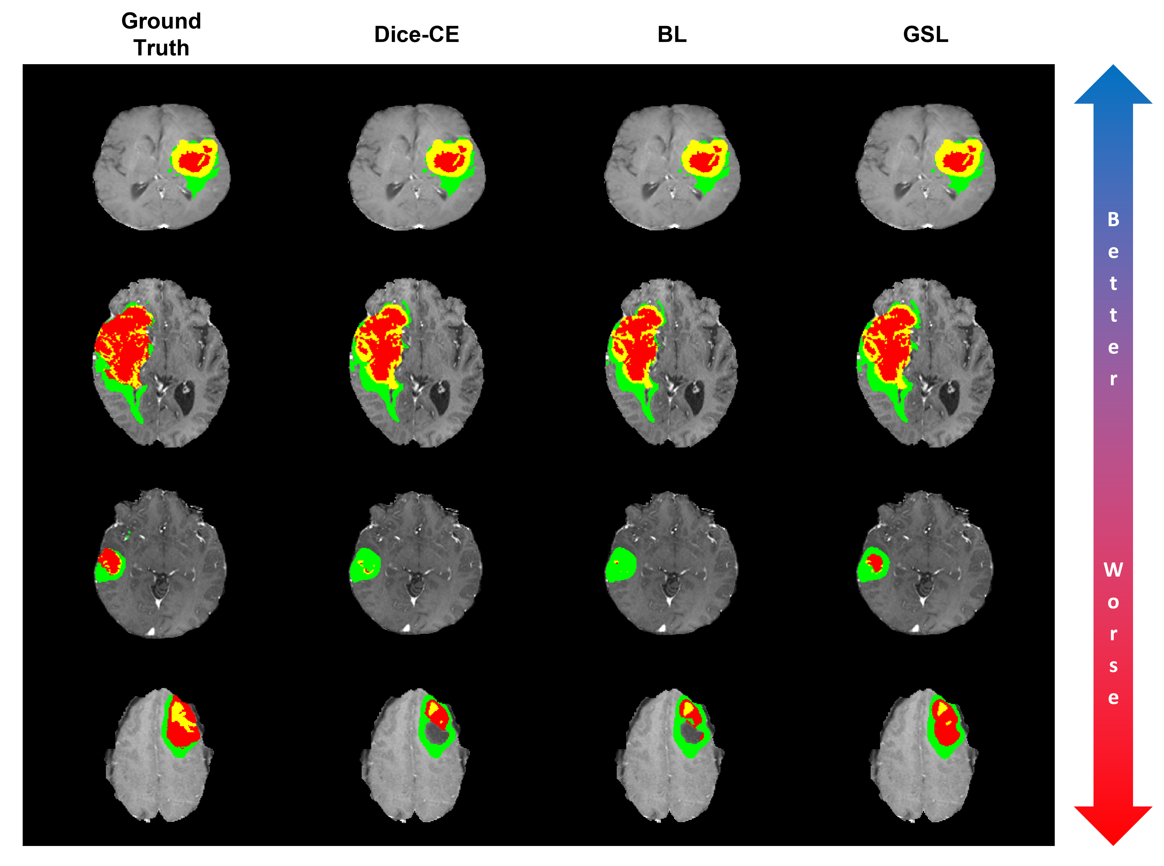
Figure 4: From left to right, ground truth and predictions from the nnUNet architecture trained on BraTS data with Dice-CE, BL, and GSL functions for a spectrum of easier to more difficult test cases. Here, we see that, even for more difficult cases, the GSL produces visually superior predictions than the Dice-CE and BL functions.

We also test our GSL with different $\alpha$-schedules. Table 2 shows each metric’s mean and standard deviation from testing different schedules for $\alpha$ with our GSL. We compare the accuracy for linear, decreasing step functions with step lengths of 5, 25, and 50 epochs and a cosine function as schedules. For the LiTS dataset, it is clear that the decreasing step function with a step length of 5 epochs achieves the best accuracy vs. the other schedules. For the BraTS dataset, the results are less clear, with the decreasing step function with a step length of 25 epochs achieving the best metrics for the Whole Tumor task, the step function with a step length of 5 epochs for the Tumor Core task, and the linear schedule for the Enhancing Tumor task.

Dataset	Task	Schedule	Dice [$\uparrow$]	Hausdorf 95 (mm) [$\downarrow$]	Avg. Surface (mm) [$\downarrow$]
LiTS	Liver	Linear	0.9302 (0.1075)	8.9046 (28.205)	3.2791 (7.0823)
		Step - 5	0.9339 (0.0983)	7.2410 (24.915)	2.6315 (5.0905)
		Step - 25	0.9302 (0.1133)	8.0823 (26.251)	3.1676 (8.5182)
		Step - 50	0.9275 (0.1107)	7.9524 (24.056)	3.1763 (6.0171)
		Cosine	0.9300 (0.1182)	13.005 (67.511)	8.2237 (63.309)
BraTS	Whole Tumor	Linear	0.9087 (0.0722)	3.5367 (9.7121)	1.1442 (1.8159)
		Step - 5	0.9081 (0.0738)	3.7796 (9.4055)	1.1552 (1.6483)
		Step - 25	0.9093 (0.0786)	2.9509 (8.4327)	1.0719 (1.7167)
		Step - 50	0.9067 (0.0775)	3.8417 (10.776)	1.2326 (2.1089)
		Cosine	0.9074 (0.0833)	3.6255 (10.140)	1.2187 (2.6784)
	Tumor Core	Linear	0.8448 (0.1835)	4.9526 (11.333)	1.8121 (4.9699)
		Step - 5	0.8439 (0.1804)	4.8878 (10.846)	1.7734 (4.6574)
		Step - 25	0.8473 (0.1795)	6.5636 (28.895)	3.5387 (27.425)
		Step - 50	0.8473 (0.1776)	5.5879 (21.672)	2.4524 (19.434)
		Cosine	0.8508 (0.1750)	5.3815 (21.941)	2.6191 (19.833)
	Enhancing Tumor	Linear	0.7587 (0.2696)	30.121 (93.228)	26.551 (93.568)
		Step - 5	0.7517 (0.2759)	31.159 (94.948)	27.521 (95.237)
		Step - 25	0.7555 (0.2739)	32.453 (98.038)	29.318 (98.554)
		Step - 50	0.7511 (0.2781)	31.863 (96.466)	28.352 (96.909)
		Cosine	0.7562 (0.2707)	31.663 (96.562)	28.352 (96.918)

Table 2: Each metric’s mean and standard deviation from testing different schedules for $\alpha$ with our GSL. We compare the accuracy for linear, decreasing step functions with step lengths of 5, 25, and 50 epochs, and a cosine function as schedules. For the LiTS dataset, the decreasing step function with a step length of 5 epochs achieves the best accuracy vs. the other schedules. For the BraTS dataset, the results are less clear, with the decreasing step function with a step length of 25 epochs achieving the best metrics for the Whole Tumor task, the step function with a step length of 5 epochs for the Tumor Core task, and the linear schedule for the Enhancing Tumor task.

4 Discussion

The results above show that our proposed GSL function is a promising alternative loss function for medical imaging segmentation tasks. The GSL outperforms other losses regarding HD and ASD accuracy on the LiTS and BraTS datasets while maintaining comparable accuracy for the Dice coefficient. The GSL predictions also generally appear to have less variance than the other losses tested. These results also suggest that the GSL function could benefit applications where HD and ASD accuracy are crucial. We hypothesize that our proposed loss function archives higher accuracy than other boundary-based loss functions partly because it is normalized to a similar scale as the region-based loss with which it is used in a weighted combination. This normalization is desirable from an optimization perspective and a desirable property for training in the presence of noise. Indeed, [10] and [30] show that normalized loss functions can improve the robustness of deep learning models with noise in the data or labels. Medical imaging data is inherently noisy, with CT images showing a degree of Gaussian noise and MR images showing Rician noise and bias fields, depending on the machine and acquisition parameters [17, 32, 14, 40].

The results in Table 2 indicate that the choice of scheduler for the weighting parameter $\alpha$ in (8). For the LiTS dataset, the choice of a decreasing step function with a step length of 5 epochs appears to be the optimal choice vs. the other schedules. However, the results are unclear for the BraTS dataset, with the linear and step functions with various step length sizes appearing to produce the most accurate result for different metrics and tumor subcomponents. The intuition governing the step function schedules is to allow the optimizer to focus on fewer subproblems during training. One can view the linear function as a decreasing step function with step length one. However, increasing the size of the step length allows optimizers like Adam to minimize each stage of the overall loss more effectively. Our results partially support this claim, but further work is needed to understand better how to select an $\alpha$-schedule optimally.

The intuition behind the GSL function is based on the properties of the segmentation images (values are in the interval $[0,1]$) and the DTM. Recall that for a given segmentation, the DTM is positive on the exterior, zero on the boundary, and negative on the object’s interior. Hence, for the given maximal value in (10), the goal of the GLS is to produce a prediction $P$ such that $D\odot(\mathbf{1}-(T+P))=|D|$, where $\odot$ is the Hadamard or pointwise product. In other words, predictions that are as close as possible to the ground truth will also recover the absolute value of the DTM. Note that we use the 2-norm instead of absolute values in our formulation. Using other norms like the 1-norm may affect the results presented above. Future work will explore developing and testing different formulations of the GSL.

While not tested in our work, the choice of region-based loss for (8) may also affect the results shown in Tables 1 and 2. In several cases in Table 1, we see that the Dice loss achieves higher accuracy than the Dice-CE loss. We may improve our results by using the Dice loss as $\mathcal{L}_{region}$. Additionally, using the precomputed weights shown in (13) for the GDL may also serve as an effective region-based loss. It may also be worth considering non-region-based losses in (8). For example, using only cross-entropy or the focal loss [26], which are considered distribution-based losses [22], could be beneficial. Testing different region (or non-region) losses will be an objective of future work.

The choice of precomputed weighting terms may be another important factor in our GSL. For example, one might also consider the weighting terms

$$w_{k}=\left(\frac{1}{\sum_{j=1}^{C}\left(\frac{1}{N_{j}}\right)^{p}}\right)\left(\frac{1}{N_{k}}\right)^{p},$$ (17)

for some $p>1$. Additionally, weighting terms based on the surface area of the given object might be advantageous for the GSL. In [42], Sugino et al. show the effectiveness for weights that depend on the DTM itself. It is also unclear how the weighting terms and the given segmentation task are related. For example, other weighting schemes might be more appropriate for different types of tumors or imaging modalities.

5 Conclusion

Our results indicate that we can improve segmentation accuracy for deep learning-based medical imaging segmentation tasks with our novel GSL function. When tested on the BraTS and LiTS datasets, the state-of-the-art nnUNet architecture trained with our proposed GSL achieved greater accuracy in the HD and ASD and comparable Dice scores. While further testing on other datasets like the Medical Segmentation Decathalon [3] is needed, we are encouraged by the level of accuracy observed in the BraTS and LiTS datasets. Future work will focus on continuing to validate our results on more diverse and complex segmentation tasks and further refining our GLS to incorporate better $\alpha$-schedules, more refined weighting terms, and optimal complementary losses in (8).

6 Acknowledgments

The Department of Defense supports Adrian Celaya through the National Defense Science & Engineering Graduate Fellowship Program. David Fuentes is partially supported by R21CA249373. Beatrice Riviere is partially supported by NSF-DMS2111459. This research was partially supported by the Tumor Measurement Initiative through the MD Anderson Strategic Research Initiative Development (STRIDE), NSF-2111147, and NSF-2111459.

References

- [1] Nabila Abraham and Naimul Mefraz Khan. A novel focal tversky loss function with improved attention u-net for lesion segmentation. In 2019 IEEE 16th international symposium on biomedical imaging (ISBI 2019), pages 683–687. IEEE, 2019.
- [2] Jonas A Actor, David T Fuentes, and Béatrice Rivière. Identification of kernels in a convolutional neural network: connections between the level set equation and deep learning for image segmentation. In Medical Imaging 2020: Image Processing, volume 11313, page 1131317. International Society for Optics and Photonics, 2020.
- [3] Michela Antonelli, Annika Reinke, Spyridon Bakas, Keyvan Farahani, Annette Kopp-Schneider, Bennett A Landman, Geert Litjens, Bjoern Menze, Olaf Ronneberger, Ronald M Summers, et al. The medical segmentation decathlon. Nature communications, 13(1):4128, 2022.
- [4] Hykoush Asaturyan, E Louise Thomas, Julie Fitzpatrick, Jimmy D Bell, and Barbara Villarini. Advancing pancreas segmentation in multi-protocol mri volumes using hausdorff-sine loss function. In Machine Learning in Medical Imaging: 10th International Workshop, MLMI 2019, Held in Conjunction with MICCAI 2019, Shenzhen, China, October 13, 2019, Proceedings 10, pages 27–35. Springer, 2019.
- [5] S Bakas and et al. Advancing the cancer genome atlas glioma mri collections with expert segmentation labels and radiomic features. Scientific Data, 4(1):170117, 2017.
- [6] S. Bakas and et al. Identifying the best machine learning algorithms for brain tumor segmentation, progression assessment, and overall survival prediction in the brats challenge. arXiv preprint arXiv:1811.02629, 2018.
- [7] Richard Beare, Bradley Lowekamp, and Ziv Yaniv. Image segmentation, registration and characterization in r with simpleitk. Journal of statistical software, 86, 2018.
- [8] Jeroen Bertels, Tom Eelbode, Maxim Berman, Dirk Vandermeulen, Frederik Maes, Raf Bisschops, and Matthew B Blaschko. Optimizing the dice score and jaccard index for medical image segmentation: Theory and practice. In Medical Image Computing and Computer Assisted Intervention–MICCAI 2019: 22nd International Conference, Shenzhen, China, October 13–17, 2019, Proceedings, Part II 22, pages 92–100. Springer, 2019.
- [9] Patrick Bilic and et al. The liver tumor segmentation benchmark (LiTS). arXiv preprint arXiv:1901.04056, 2019.
- [10] Sebastian Braun and Ivan Tashev. Data augmentation and loss normalization for deep noise suppression. In International Conference on Speech and Computer, pages 79–86. Springer, 2020.
- [11] M Jorge Cardoso, Wenqi Li, Richard Brown, Nic Ma, Eric Kerfoot, Yiheng Wang, Benjamin Murrey, Andriy Myronenko, Can Zhao, Dong Yang, et al. Monai: An open-source framework for deep learning in healthcare. arXiv preprint arXiv:2211.02701, 2022.
- [12] Adrian Celaya, Jonas A Actor, Rajarajesawari Muthusivarajan, Evan Gates, Caroline Chung, Dawid Schellingerhout, Beatrice Riviere, and David Fuentes. Pocketnet: A smaller neural network for medical image analysis. IEEE Transactions on Medical Imaging, 42(4):1172–1184, 2022.
- [13] Özgün Çiçek, Ahmed Abdulkadir, Soeren S Lienkamp, Thomas Brox, and Olaf Ronneberger. 3d u-net: learning dense volumetric segmentation from sparse annotation. In Medical Image Computing and Computer-Assisted Intervention–MICCAI 2016: 19th International Conference, Athens, Greece, October 17-21, 2016, Proceedings, Part II 19, pages 424–432. Springer, 2016.
- [14] Pierrick Coupé, José V Manjón, Elias Gedamu, Douglas Arnold, Montserrat Robles, and D Louis Collins. Robust rician noise estimation for mr images. Medical image analysis, 14(4):483–493, 2010.
- [15] William R Crum, Oscar Camara, and Derek LG Hill. Generalized overlap measures for evaluation and validation in medical image analysis. IEEE transactions on medical imaging, 25(11):1451–1461, 2006.
- [16] Lee R Dice. Measures of the amount of ecologic association between species. Ecology, 26(3):297–302, 1945.
- [17] Manoj Diwakar and Manoj Kumar. A review on ct image noise and its denoising. Biomedical Signal Processing and Control, 42:73–88, 2018.
- [18] E. Ermis and et al. Fully automated brain resection cavity delineation for radiation target volume definition in glioblastoma patients using deep learning. Radiation Oncology, 15:1–10, 5 2020.
- [19] Nicholas Heller, Fabian Isensee, Klaus H Maier-Hein, Xiaoshuai Hou, Chunmei Xie, Fengyi Li, Yang Nan, Guangrui Mu, Zhiyong Lin, Miofei Han, et al. The state of the art in kidney and kidney tumor segmentation in contrast-enhanced ct imaging: Results of the kits19 challenge. Medical image analysis, 67:101821, 2021.
- [20] Fabian Isensee, Paul F. Jaeger, Simon A.A. Kohl, Jens Petersen, and Klaus H. Maier-Hein. nnu-net: a self-configuring method for deep learning-based biomedical image segmentation. Nature Methods 2020 18:2, 18:203–211, 12 2020.
- [21] Fabian Isensee, Paul F. Jäger, Peter M. Full, Philipp Vollmuth, and Klaus H. Maier-Hein. nnu-net for brain tumor segmentation. In Alessandro Crimi and Spyridon Bakas, editors, Brainlesion: Glioma, Multiple Sclerosis, Stroke and Traumatic Brain Injuries, pages 118–132, Cham, 2021. Springer International Publishing.
- [22] Shruti Jadon. A survey of loss functions for semantic segmentation. In 2020 IEEE conference on computational intelligence in bioinformatics and computational biology (CIBCB), pages 1–7. IEEE, 2020.
- [23] Davood Karimi and Septimiu E. Salcudean. Reducing the hausdorff distance in medical image segmentation with convolutional neural networks. IEEE Transactions on Medical Imaging, 39(2):499–513, 2020.
- [24] Hoel Kervadec, Jihene Bouchtiba, Christian Desrosiers, Eric Granger, Jose Dolz, and Ismail Ben Ayed. Boundary loss for highly unbalanced segmentation. Medical image analysis, 67:101851, 2021.
- [25] Shen Li, Yanli Zhao, Rohan Varma, Omkar Salpekar, Pieter Noordhuis, Teng Li, Adam Paszke, Jeff Smith, Brian Vaughan, Pritam Damania, et al. Pytorch distributed: Experiences on accelerating data parallel training. arXiv preprint arXiv:2006.15704, 2020.
- [26] Tsung-Yi Lin, Priya Goyal, Ross Girshick, Kaiming He, and Piotr Dollár. Focal loss for dense object detection. In Proceedings of the IEEE international conference on computer vision, pages 2980–2988, 2017.
- [27] Bingyuan Liu, Jose Dolz, Adrian Galdran, Riadh Kobbi, and Ismail Ben Ayed. Do we really need dice? the hidden region-size biases of segmentation losses. Medical Image Analysis, page 103015, 2023.
- [28] Bradley C Lowekamp, David T Chen, Luis Ibáñez, and Daniel Blezek. The design of simpleitk. Frontiers in neuroinformatics, 7:45, 2013.
- [29] Jun Ma, Jianan Chen, Matthew Ng, Rui Huang, Yu Li, Chen Li, Xiaoping Yang, and Anne L Martel. Loss odyssey in medical image segmentation. Medical Image Analysis, 71:102035, 2021.
- [30] Xingjun Ma, Hanxun Huang, Yisen Wang, Simone Romano, Sarah Erfani, and James Bailey. Normalized loss functions for deep learning with noisy labels. In International conference on machine learning, pages 6543–6553. PMLR, 2020.
- [31] Calvin R Maurer, Rensheng Qi, and Vijay Raghavan. A linear time algorithm for computing exact euclidean distance transforms of binary images in arbitrary dimensions. IEEE Transactions on Pattern Analysis and Machine Intelligence, 25(2):265–270, 2003.
- [32] Rini Mayasari and Nono Heryana. Reduce noise in computed tomography image using adaptive gaussian filter. arXiv preprint arXiv:1902.05985, 2019.
- [33] B Menze and et al. The multimodal brain tumor image segmentation benchmark (brats). IEEE Transactions on Medical Imaging, 34(10):1993–2024, 2015.
- [34] Fausto Milletari, Nassir Navab, and Seyed-Ahmad Ahmadi. V-net: Fully convolutional neural networks for volumetric medical image segmentation. In 2016 Fourth International Conference on 3D Vision (3DV), pages 565–571, 2016.
- [35] Frederic Morain-Nicolier, Stephane Lebonvallet, Etienne Baudrier, and Su Ruan. Hausdorff distance based 3d quantification of brain tumor evolution from mri images. In 2007 29th Annual International Conference of the IEEE Engineering in Medicine and Biology Society, pages 5597–5600, 2007.
- [36] Adam Paszke, Sam Gross, Francisco Massa, Adam Lerer, James Bradbury, Gregory Chanan, Trevor Killeen, Zeming Lin, Natalia Gimelshein, Luca Antiga, et al. Pytorch: An imperative style, high-performance deep learning library. Advances in neural information processing systems, 32, 2019.
- [37] Olaf Ronneberger, Philipp Fischer, and Thomas Brox. U-net: Convolutional networks for biomedical image segmentation. In Medical Image Computing and Computer-Assisted Intervention–MICCAI 2015: 18th International Conference, Munich, Germany, October 5-9, 2015, Proceedings, Part III 18, pages 234–241. Springer, 2015.
- [38] Seyed Sadegh Mohseni Salehi, Deniz Erdogmus, and Ali Gholipour. Tversky loss function for image segmentation using 3d fully convolutional deep networks. In International workshop on machine learning in medical imaging, pages 379–387. Springer, 2017.
- [39] Neeraj Sharma, Lalit M Aggarwal, et al. Automated medical image segmentation techniques. Journal of medical physics, 35(1):3, 2010.
- [40] Jamuna Kanta Sing, Sudip Kumar Adhikari, and Sayan Kahali. On estimation of bias field in mri images. In 2015 IEEE International Conference on Computer Graphics, Vision and Information Security (CGVIS), pages 269–274. IEEE, 2015.
- [41] Carole H Sudre, Wenqi Li, Tom Vercauteren, Sebastien Ourselin, and M Jorge Cardoso. Generalised dice overlap as a deep learning loss function for highly unbalanced segmentations. In Deep Learning in Medical Image Analysis and Multimodal Learning for Clinical Decision Support: Third International Workshop, DLMIA 2017, and 7th International Workshop, ML-CDS 2017, Held in Conjunction with MICCAI 2017, Québec City, QC, Canada, September 14, Proceedings 3, pages 240–248. Springer, 2017.
- [42] Takaaki Sugino, Toshihiro Kawase, Shinya Onogi, Taichi Kin, Nobuhito Saito, and Yoshikazu Nakajima. Loss weightings for improving imbalanced brain structure segmentation using fully convolutional networks. In Healthcare, volume 9, page 938. MDPI, 2021.
- [43] Saeid Asgari Taghanaki, Yefeng Zheng, S Kevin Zhou, Bogdan Georgescu, Puneet Sharma, Daguang Xu, Dorin Comaniciu, and Ghassan Hamarneh. Combo loss: Handling input and output imbalance in multi-organ segmentation. Computerized Medical Imaging and Graphics, 75:24–33, 2019.
- [44] Abdel Aziz Taha and Allan Hanbury. Metrics for evaluating 3d medical image segmentation: analysis, selection, and tool. BMC medical imaging, 15(1):1–28, 2015.
- [45] David Thomson, Chris Boylan, Tom Liptrot, Adam Aitkenhead, Lip Lee, Beng Yap, Andrew Sykes, Carl Rowbottom, and Nicholas Slevin. Evaluation of an automatic segmentation algorithm for definition of head and neck organs at risk. Radiation Oncology, 9(1):1–12, 2014.
- [46] Ken CL Wong, Mehdi Moradi, Hui Tang, and Tanveer Syeda-Mahmood. 3d segmentation with exponential logarithmic loss for highly unbalanced object sizes. In Medical Image Computing and Computer Assisted Intervention–MICCAI 2018: 21st International Conference, Granada, Spain, September 16-20, 2018, Proceedings, Part III 11, pages 612–619. Springer, 2018.
- [47] Ziv Yaniv, Bradley C Lowekamp, Hans J Johnson, and Richard Beare. Simpleitk image-analysis notebooks: a collaborative environment for education and reproducible research. Journal of digital imaging, 31(3):290–303, 2018.
- [48] Hongyan Zhu, Shuni Song, Lisheng Xu, Along Song, and Benqiang Yang. Segmentation of coronary arteries images using spatio-temporal feature fusion network with combo loss. Cardiovascular Engineering and Technology, pages 1–12, 2022.
- [49] Wentao Zhu, Yufang Huang, Liang Zeng, Xuming Chen, Yong Liu, Zhen Qian, Nan Du, Wei Fan, and Xiaohui Xie. Anatomynet: deep learning for fast and fully automated whole-volume segmentation of head and neck anatomy. Medical physics, 46(2):576–589, 2019.