$g$-mode of neutron stars in pseudo-Newtonian gravity

Abstract

The equation of state (EOS) of nuclear dense matter plays a crucial role in many astrophysical phenomena associated with neutron stars (NSs). Fluid oscillations are one of the most fundamental properties therein. NSs support a family of gravity $g$-modes, which are related to buoyancy. We study the gravity $g$-modes caused by composition gradient and density discontinuity in the framework of pseudo-Newtonian gravity. The mode frequencies are calculated in detail and compared with Newtonian and general-relativistic (GR) solutions. We find that the $g$-mode frequencies in one of the pseudo-Newtonian treatments can approximate remarkably well the GR solutions, with relative errors in the order of $1\%$. Our findings suggest that, with much less computational cost, pseudo-Newtonian gravity can be utilized to accurately analyze oscillation of NSs constructed from an EOS with a first-order phase transition between nuclear and quark matter, as well as to provide an excellent approximation of GR effects in core-collapse supernova (CCSN) simulations.

I Introduction

The oscillation modes of neutron stars (NSs) provide a means to probe the internal composition and state of dense matter. NSs have rich oscillation spectra, with modes associated with different physical origins, such as the internal ingredients, the elasticity of the crust, superfluid components, and so on [1]. For typical non-rotating fluid stars, the oscillation modes include the fundamental ($f$), pressure ($p$), and gravity ($g$) modes, which provided the basic classification of modes according to the physics dominating their behaviours [2]. More realistic stellar models and rotation introduce additional classes of oscillation modes.

In this work, we study the $g$-mode oscillations for non-rotating NSs in the framework of pseudo-Newtonian gravity [3, 4, 5, 6, 7, 8, 9, 10]. Reisenegger and Goldreich [11] investigated the $g$-mode induced by composition (proton-to-neutron ratio) gradient in the cores of NSs. Moreover, hot young NSs may excite $g$-modes supported by entropy gradients [12, 13, 14, 15]. It has also been demonstrated that the onset of superfluidity has a key influence on the buoyancy that supports the $g$-modes [16, 17, 18, 19, 20]. Density discontinuity produced by abrupt composition transitions may play an important role in determining the $g$-mode properties [21, 22]. Sotani et al. [23] calculated $f$ and $g$ modes of NSs with density discontinuity at an extremely high density and discussed the stability of the stellar models. A phase transition occurred in the cores of NSs with a polytropic equation of state (EOS) has been studied by Miniutti et al. [24]. The frequencies of $g$-modes from density discontinuity are larger than those induced by the entropy gradient. Furthermore, discontinuity $g$-mode may occur in perturbed quark-hadron hybrid stars [25, 26]. Recently, Zhao et al. [27] considered the $g$-mode of NSs containing quark matter and discussed the Cowling approximation, which leads to a relative error of $\sim 10\%$ for higher-mass hybrid stars. We here focus on the $f$ and $g$ modes of NSs in pseudo-Newtonian gravity caused by the first-order phase transition in the cores of NSs.

The study of NS oscillations is timely in the gravitational-wave era [28, 29, 30]. Tidal interaction in a coalescing binary NS can resonantly excite the $g$-mode oscillation of NSs when the frequency of the tidal driving force approaches the $g$-mode frequencies [31, 32]. Moreover, the mixture of pure-inertial and inertial-gravity modes can become resonantly excited by tidal fields for rotating NSs [33, 34]. The $g$-mode can also result in secular instability in rotating NSs [35]. Gaertig and Kokkotas [36] considered the $g$-mode of fast-rotating stratified NSs using the relativistic Cowling approximation. The typical scenarios pertain to the $p$-$g$ mode instability and the saturation of unstable modes [37, 38]. The universal relation of $g$-mode asteroseismology has been discussed by Kuan et al. [39] for different classes of EOSs. In particular, the absence of very low-frequency $g$-modes helps to explain the absence of tidal resonances [40]. The cut-off in the high-order $g$-mode spectrum may also be relevant for scenarios of nonlinear mode coupling. The properties of $g$-modes for newly-born strange quark stars and NSs using Cowling approximation in Newtonian gravity have been discussed by Fu et al. [41].

Hydrodynamical simulations are necessary to study the properties of the proto-NS in a core-collapse supernova (CCSN). The $g$-mode of such a scenario may impact associated gravitational waves [42]. However, the physics of neutrino transport and EOS is very uncertain for the hydrodynamical simulations. As multi-dimensional general-relativistic (GR) codes for numerical simulations are scarce and have high demand of computational cost, most previous investigations relied on the Newtonian approximation for the strong gravitational field and fluid dynamics [3, 4]. Nevertheless, “Case A potential” formalism (c.f. Sec. II.1) was found to be a good approximation to relativistic solutions in simulating non-rotating or slowly rotating CCSNs. This potential allows for an accurate approximation of GR effects in an otherwise Newtonian hydrodynamic code, and it also works for cases of rapid rotation [4]. This has motivated a sequence of CCSN simulations [5, 6, 7, 8]. The effectiveness of using Case A potential formalism to approximate GR has been studied by Mueller et al. [4], Pajkos et al. [43], O’Connor et al. [7]. In particular, Mueller et al. [4] found that Case A potential formalism can not obtain the correct oscillation modes and indicated the failure of the Case A potential, possibly being attributed to the absence of a lapse function. Recently, Zha et al. [9] have extended the Case A potential formalism with a lapse function to simulate the oscillation of proto-neutron star (PNS). They found that Case A potential formalism with an additional lapse function can approximate well the frequency of the fundamental radial mode.

Tang and Lin [10] studied the radial and non-radial oscillation modes of NSs in pseudo-Newtonian gravity, including the Case A potential with and without the lapse function. Motivated by Tang and Lin [10], we here study the $g$-mode of NS cores using Case A potential formalism with and without the lapse function. Our findings suggest that, with much less computational cost, pseudo-Newtonian gravity can be utilized to accurately analyze oscillation of NSs constructed from an EOS with a first-order phase transition, thus to provide an excellent approximation of GR effects in CCSN simulations.

The paper is organized as follows. In Sec. II, we introduce the key ingredients of the model, including different pseudo-Newtonian schemes and the buoyancy nature associated with $g$-mode. The local dynamics of NS cores, including composition gradient and density discontinuity, are presented in Sec. III. Finally, we summarize our work in Sec. IV. Throughout the paper, we adopt geometric units with $c=G=1$, where $c$ and $G$ are the speed of light and the gravitational constant, respectively.

II Key ingredients of the model

II.1 Case A potential in pseudo-Newtonian gravity

Case A effective potential is defined by replacing the Newtonian gravitational potential in a spherically symmetric Newtonian hydrodynamic simulation by [3, 10]

$$\Phi_{\rm TOV}(r)=-4\pi\int^{\infty}_{r}\frac{\mathrm{d}r^{\prime}}{r^{\prime 2}}\left(\frac{m_{\rm TOV}}{4\pi}+r^{\prime 3}P\right)\times\frac{1}{\Gamma^{2}}\left(\frac{\rho+\rho\varrho+P}{\rho}\right)\,,$$ (1)

where $r$ is the radial coordinate, $\rho$ is the rest-mass density, $P$ is the pressure, $\varrho$ is the specific internal energy, and the total energy density is given by $\epsilon=\rho+\rho\varrho$. The function $m_{\text{TOV}}$ is defined by

$$m_{\rm TOV}(r)=4\pi\int^{r}_{0}\mathrm{d}r^{\prime}r^{\prime 2}\epsilon\Gamma\,,$$ (2)

with

$$\Gamma=\sqrt{1-2\frac{m_{\rm TOV}}{r}}\,.$$ (3)

From Eq. (1) and Eq. (2), we have

$$\frac{{\rm d}m_{\rm TOV}}{{\rm d}r} =4\pi r^{2}\epsilon\Gamma\,,$$ (4)

$$\frac{{\rm d}\Phi_{\rm TOV}}{{\rm d}r} =\frac{4\pi}{r^{2}}\left(\frac{m_{\rm TOV}}{4\pi}+r^{3}P\right)\frac{1}{\Gamma^{2}}\frac{(\epsilon+P)}{\rho}\,.$$ (5)

We use the Case A and Case A+lapse schemes and the other four schemes to study the $g$-mode originating from the composition gradient and density discontinuity of NS cores in the framework of pseudo-Newtonian gravity. All background and perturbation equations for each scheme are given in the next three subsections and summarized in Table 1.

Table 1: Different schemes to calculate the oscillation modes, along with the corresponding background and the lapse function. Non-radial perturbation equations are the same [Eqs. (28–31)] for all six schemes, but some of them include a lapse-function $\alpha$ in the hydrodynamic equations. Note that the lapse function only appears in the perturbation equations but not in the background equations.

Scheme	Background equations	Lapse function $\alpha$
N	Eqs. (6) to (8)	–
N+lapse	Eqs. (6) to (8)	Eq. (17)
TOV	Eqs. (9) to (11)	–
TOV+lapse	Eqs. (9) to (11)	Eq. (17)
Case A	Eqs. (12) to (14)	–
Case A+lapse	Eqs. (12) to (14)	Eq. (17)

II.2 Equilibrium configurations

We consider the following three sets of equilibrium configurations.

1. For the Newtonian (N) and Newtonian+lapse function (N+lapse) schemes, the hydrostatic equilibrium equations are

   $$\frac{{\rm d}m}{{\rm d}r} =4\pi r^{2}\rho\,,$$ (6)

   $$\frac{{\rm d}P}{{\rm d}r} =-\frac{\rho m}{r^{2}}\,,$$ (7)

   $$\frac{{\rm d}\Phi}{{\rm d}r} =-\frac{1}{\rho}\frac{{\rm d}P}{{\rm d}r}\,.$$ (8)

   where $\rho$ is the rest-mass density, and $\Phi$ is the Newtonian gravitational potential.

2. Instead, if we consider spherical and static stars in GR, we have the Tolman-Oppenheimer-Volkoff (TOV) equations

   $$\frac{{\rm d}m}{{\rm d}r} =4\pi r^{2}\epsilon\,,$$ (9)

   $$\frac{{\rm d}P}{{\rm d}r} =-\frac{(\epsilon+P)(m+4\pi r^{3}P)}{r(r-2m)}\,,$$ (10)

   $$\frac{{\rm d}\Phi}{{\rm d}r} =-\frac{1}{\epsilon+P}\frac{{\rm d}P}{{\rm d}r}\,.$$ (11)

3. Lastly, for the Case A and Case A+lapse schemes, the background equations are obtained by replacing the Newtonian gravitational potential by the Case A potential [3, 10], and we have

   $$\frac{{\rm d}m}{{\rm d}r} =4\pi r^{2}\epsilon\Gamma\,,$$ (12)

   $$\frac{{\rm d}P}{{\rm d}r} =-\frac{4\pi}{r^{2}}\left(\frac{m}{4\pi}+r^{3}P\right)\frac{1}{\Gamma^{2}}(\epsilon+P)\,,$$ (13)

   $$\frac{{\rm d}\Phi}{{\rm d}r} =-\frac{1}{\rho}\frac{\mathrm{d}P}{\mathrm{d}r}\,.$$ (14)

We use the modified Newtonian hydrodynamic equations in Zha et al. [9] and Tang and Lin [10], where a lapse function $\alpha$ is added to mimic the time-dilation effect. The modified hydrodynamic equations are:

$$\frac{\partial\rho}{\partial t}+\nabla\cdot(\alpha\rho\vec{v})=0,$$ (15)

$$\frac{\partial}{\partial t}(\rho\vec{v})+\nabla\cdot[\alpha(\rho\vec{v}\vec{v}+P\overset{\leftrightarrow}{I})]=-\alpha(\rho-P)\nabla\Phi\,,$$ (16)

where $\vec{v}$ is the fluid velocity and the lapse function is defined by

$$\alpha=\exp(\Phi)\,.$$ (17)

The readers can infer Tang and Lin [10] for a detailed variational derivation of the linearized fluid equations. We will use the same lapse function in our calculations.

II.3 Buoyancy and the $g$-mode

As well known that NSs always have real frequency $f$-mode and $p$-mode regimes. However, $g$-mode may have a real, imaginary, and zero frequency, which correspond to convective stability, instability, and marginal stability. We consider the local dynamics of NS cores, focusing on the buoyancy experienced by fluid elements and the associated $g$-mode. The frequencies of $g$-modes are closely related to the Brunt-Väisälä frequency $N$, defined via

$$N^{2}=g_{N}^{2}\left(\frac{1}{c_{\mathrm{e}}^{2}}-\frac{1}{c_{\mathrm{s}}^{2}}\right)\,,$$ (18)

where $g_{N}$ is the positive Newtonian gravitational acceleration, $c_{\mathrm{s}}$ is the adiabatic sound speed,

$$c_{\mathrm{s}}^{2}=\left(\frac{\partial P}{\partial\rho}\right)_{\mathrm{s}}\,.$$ (19)

Here the subscript “s” means “adiabatic”, which in this case implies constant composition. The quantity $c_{\mathrm{e}}$ is given by

$$c_{\mathrm{e}}^{2}=\frac{{\rm d}P}{{\rm d}\rho}\,,$$ (20)

where the subscript “e” stands for “equilibrium”. If $c_{\mathrm{s}}^{2}=c_{\mathrm{e}}^{2}$, the star exhibits no convective phenomena (zero-buoyancy case). In this work, we consider only the $g$-mode of NS cores, so we set $c_{\mathrm{s}}^{2}=c_{\mathrm{e}}^{2}$ for the crustal region. Again, $c_{\mathrm{s}}^{2}>c_{\mathrm{e}}^{2}$ ($c_{\mathrm{s}}^{2}<c_{\mathrm{e}}^{2}$) denotes convective stability (instability). Combining Eqs. (18–20), we can write the Brunt-Väisälä frequency as

$$N^{2}=-Ag_{N}\,,$$ (21)

where $A$ is

$$A=\frac{{\rm d}\ln\rho}{{\rm d}r}-\frac{1}{\Gamma_{1}}\frac{{\rm d}\ln P}{{\rm d}r}\,,$$ (22)

which is called the Schwarzschild discriminant. If the star model obeys a simple polytropic EOS, $P=K\rho^{\gamma}$, then $\gamma=\rm d\ln P/\rm d\ln\rho$ is defined for the unperturbed background configuration. Hence, the Schwarzschild discriminant becomes

$$A=\left(\frac{1}{\gamma}-\frac{1}{\Gamma_{1}}\right)\frac{{\rm d}\ln P}{{\rm d}r}\,.$$ (23)

Clearly, if the adiabatic index $\Gamma_{1}>\gamma$, the star is related to the convective stability, in the case of $c_{\mathrm{s}}^{2}>c_{\mathrm{e}}^{2}$. In Sec. III.1, we will calculate the frequencies of $g$-modes for the composition gradient, which is related to the discussion here.

II.4 Non-radial perturbation equations

In this section, we study non-radial oscillations of NSs in pseudo-Newtonian gravity. Tang and Lin [10] calculated the quadrupole ($\ell=2$) $f$ and $p$ modes. The perturbation of scalars is expanded in spherical harmonics and the Lagrangian displacement is expanded in vector spherical harmonics [13, 10]. When considering an eigenmode, we have

$$\delta\rho=\delta\tilde{\rho}(r)Y_{\ell m}\,,$$ (24)

$$\delta P=\delta\tilde{P}(r)Y_{\ell m}\,,$$ (25)

$$\delta\Phi=\delta\tilde{\Phi}(r)Y_{\ell m}\,,$$ (26)

$$\vec{\xi}=U(r)Y_{\ell m}{\hat{r}}+V(r)\nabla Y_{\ell m}\,,$$ (27)

where $Y_{\ell m}$ is the standard spherical harmonic function, and $\hat{r}$ is the radial unit vector. Then one can obtain the following system of equations for the fluid perturbations (see Tang and Lin [10], for a detailed variational derivation),

$$\frac{{\rm d}U}{{\rm d}r} =-\left(\frac{2}{r}+\frac{{\rm d}\Phi}{{\rm d}r}+\frac{1}{\gamma P}\frac{{\rm d}P}{{\rm d}r}-\frac{A}{\alpha}\right)U+\left[\frac{\alpha\ell(\ell+1)}{\rho r^{2}\omega^{2}}-\frac{1}{\alpha\Gamma_{1}P}\right]\delta\tilde{P}$$

$$\quad+\frac{\alpha\ell(\ell+1)}{r^{2}\omega^{2}}\delta\tilde{\Phi}\,,$$ (28)

$$\frac{{\rm d}\delta\tilde{P}}{{\rm d}r} =\left(\frac{\rho\omega^{2}}{\alpha}-\frac{{\rm d}P}{{\rm d}r}A\right)U+\frac{1}{\Gamma_{1}P}\frac{{\rm d}P}{{\rm d}r}\delta\tilde{P}-\rho\frac{{\rm d}\delta\tilde{\Phi}}{{\rm d}r}\,,$$ (29)

$$\frac{{\rm d}\delta\tilde{\Phi}}{{\rm d}r} =\Psi\,,$$ (30)

$$\frac{{\rm d}\Psi}{{\rm d}r} =-\frac{2}{r}\Psi+\frac{\ell(\ell+1)}{r^{2}}\delta\tilde{\Phi}+4\pi\frac{\rho}{\Gamma_{1}P}\delta\tilde{P}-4\pi\rho AU\,.$$ (31)

To solve these equations, we require the boundary conditions at the center and surface of the NS. At the center, the regularity conditions of the variables yield the following relations [44, 10]

$$U=r^{\ell-1}A_{0}\,,$$ (32)

$$\delta\tilde{P}=r^{\ell}B_{0}\,,$$ (33)

$$\delta\tilde{\Phi}=r^{\ell}C_{0}\,,$$ (34)

$$\Psi=\ell r^{\ell-1}C_{0}\,,$$ (35)

$$A_{0}=\frac{\alpha\ell}{\rho\omega^{2}}(B_{0}+\rho C_{0})\,,$$ (36)

where $B_{0}$ and $C_{0}$ are constants. At the surface of the star, the perturbed pressure must vanish, which provides

$$\frac{{\rm d}P}{{\rm d}r}U+\delta\tilde{P}=0\,.$$ (37)

The $\delta\tilde{\Phi}$ and ${{\rm d}\delta\tilde{\Phi}}/{{\rm d}r}$ are continuous, so we obtain

$$\Psi=-\frac{\ell+1}{r}\delta\tilde{\Phi}\,.$$ (38)

Note that in the N, Case A, and TOV schemes, the lapse function equals to 1 ($\alpha=1$).

Table 2: Comparison of the non-radial mode frequencies (unit: Hz) of a polytropic star model where polytropic index $\gamma=2$, $K=1.4553\times 10^{5}\ \rm g^{-1}\,cm^{5}\,s^{-2}$, and central density $\rho_{c}=7.9\times 10^{14}\ \rm g\,cm^{-3}$, to earlier results of Westernacher-Schneider [44] and Tang and Lin [10].

Mode	Westernacher-Schneider [44]	Tang and Lin [10]	$\Gamma_{1}=2.01$	$\Gamma_{1}=2.05$	$\Gamma_{1}=2.1$	$\Gamma_{1}=2.15$
$p_{2}$	7290	7932	7957	8049	8163	8276
$p_{1}$	5122	5131	5151	5216	5297	5377
$f$	2024	2021	2021	2025	2029	2032
$g_{1}$	–	–	143	317	441	532
$g_{2}$	–	–	99	219	306	369
$g_{3}$	–	–	76	169	235	284

To test our numerical code, we have redone calculations with the same polytropic EOS as that in the Appendix A of Marek et al. [3], where the polytropic index $\gamma$ and the adiabatic index $\Gamma_{1}>\gamma$ are constant throughout the stellar interior. Detailed numerical results are shown in Table 2. It is noted that our numerical results for the polytropic model with $\Gamma_{1}=\gamma$ agree with Table 3 of Tang and Lin [10]. In Table 2, we compare the frequencies of $p$, $f$, and $g$ modes computed with $\Gamma_{1}>\gamma$ and $\Gamma_{1}=\gamma$ [44, 10]. The frequencies of $p$ and $f$ modes increase with the increase of the adiabatic index $\Gamma_{1}$. In particular, the $g$-mode frequencies also increase with increase of the adiabatic index $\Gamma_{1}$, which indicates a larger buoyancy.

III NUMERICAL RESULTS

III.1 Composition gradient

Taking the matter composition into account, and assuming that the model accounts for the presence of neutrons, protons, and electrons, we have a two-parameter EOS, $P=P(n,x)$, which is a function of the baryon number density $n$ and the proton fraction $x=n_{\mathrm{p}}/n$. Specifically, we use shorthand notations: “$\mathrm{n}$” for neutrons, “$\mathrm{p}$” for protons, and “$\mathrm{e}$” for electrons. The energy per baryon of the nuclear matter can be written as [45, 46, 47, 31]

$$E_{n}(n,x)=T_{n}(n,x)+V_{0}(n)+V_{2}(n)(1-2x)^{2}\,,$$ (39)

where

$$T_{n}(n,x)={\frac{3}{5}\frac{\hbar^{2}}{2m_{\mathrm{n}}}(3\pi^{2}n)^{2/3}[x^{5/3}}+(1-x)^{5/3}]\,,$$ (40)

is the Fermi kinetic energy of the nucleons, and $m_{n}$ is the nucleon mass. $V_{0}$ mainly specifies the bulk compressibility of the matter, and $V_{2}$ is related to the symmetry energy of nuclear matter [48].

To compare the results of $g$-modes in Newtonian gravity [31], we adopt the same $V_{0}$ and $V_{2}$ for different EOS models, based on the microscopic calculations in Wiringa et al. [47]. Detailed numerical results of $V_{0}$ and $V_{2}$ have been tabulated in Table IV of Wiringa et al. [47]. The approximate formulae of $V_{0}$ and $V_{2}$ are presented in Sec. 4.3 of Lai [31].

In this work, we consider the model “AU” (the EOS based on nuclear potential AV14+UVII in Wiringa et al. [47]) and the model “UU” (the EOS based on nuclear potential UV14+UVII in Wiringa et al. [47]), respectively. For the model AU, $V_{0}$ and $V_{2}$ (in the unit of MeV) are fitted as [31]

$$V_{0} =-43+330\,(n-0.34)^{2}\,,$$ (41)

$$V_{2} =21\,n^{0.25}\,,$$ (42)

where $n$ is the baryon number density in $\rm fm^{-3}$. For the model UU, we have

$$V_{0} =-40+400\,(n-0.3)^{2}\,,$$ (43)

$$V_{2} =42\,n^{0.55}\,.$$ (44)

These fitting formulae are valid for $0.07\,{\rm fm}^{-3}\leq n\leq 1\,\rm fm^{-3}$. For densities $0.001\,{\rm fm}^{-3}<n<0.07\,\rm fm^{-3}$, we employ the EOS of Baym et al. [49], while for $n\leq 0.001\,\rm fm^{-3}$, we employ the EOS of Baym et al. [50].

Once we have this relation, we can work out the mass-energy density, pressure, and adiabatic sound speed. The equilibrium configuration must satisfy the beta equilibrium,

$$\mu_{\mathrm{n}}=\mu_{\mathrm{p}}+\mu_{\mathrm{e}}\,,$$ (45)

and the charge neutrality

$$n_{\mathrm{p}}=n_{\mathrm{e}}\,,$$ (46)

where $\mu_{i}$ are the chemical potentials of the three species of particles. The equilibrium proton fraction $x(n)=x_{\mathrm{e}}(n)$ can be obtained by solving Eqs. (4.12–4.14) of Lai [31]. Hence, the mass-energy density and pressure are determined as

$$\epsilon(n,x) =n\big{[}m_{n}+E(n,x)/c^{2}\big{]}\,,$$ (47)

$$P(n,x) =n^{2}{\frac{\partial E(n,x)}{\partial n}}=\frac{2n}{3}T_{n}+\frac{n}{3}T_{\mathrm{e}}+n^{2}\left[V_{0}^{\prime}+V_{2}^{\prime}\,(1-2x)^{2}\right]\,,$$ (48)

where

$$T_{\mathrm{e}}(n,x_{\mathrm{e}})=\frac{3}{4}\hbar c(3\pi^{2}n)^{1/3}x_{\mathrm{e}}^{4/3}\,,$$ (49)

is the energy per baryon of relativistic electrons. Here, and in the following, primes denote baryon number density $n$ derivatives (for example, $V_{0}^{\prime}={\rm d}V_{0}/{{\rm d}n}$). The adiabatic sound speed $c_{\mathrm{s}}^{2}$ is

$$c_{\mathrm{s}}^{2}=\frac{\partial P}{\partial\epsilon}=\frac{n}{\epsilon+P/c^{2}}\frac{\partial P}{\partial n}\\ \quad=\frac{n}{\epsilon+P/c^{2}}\left\{{\frac{10}{9}}T_{n}+{\frac{4}{9}}T_{\mathrm{e}}+2n\left[V_{0}^{\prime}+V_{2}^{\prime}\,(1-2x)^{2}\right]\right\}\\ +\frac{n}{\epsilon+P/c^{2}}\left\{n^{2}\left[V_{0}^{\prime\prime}+V_{2}^{\prime\prime}\,(1-2x)^{2}\right]\right\}\,.$$ (50)

The difference between $c_{\mathrm{s}}^{2}$ and $c_{\mathrm{e}}^{2}$ is given by

$$c_{\mathrm{s}}^{2}-c_{\mathrm{e}}^{2}=\frac{n}{\epsilon+P/c^{2}}\left(\frac{\partial P}{\partial n}-\frac{{\rm d}P}{{\rm d}n}\right)=-\frac{n}{\epsilon+P/c^{2}}\left(\frac{\partial P}{\partial x}\right){\frac{{\rm d}x}{{\rm d}n}}\\ =-\frac{n^{3}}{\epsilon+P/c^{2}}\left[{\frac{\partial}{\partial n}}(\mu_{\mathrm{e}}+\mu_{\mathrm{p}}-\mu_{\mathrm{n}})\right]{\frac{{\rm d}x}{{\rm d}n}}\,.$$ (51)

From the beta equilibrium [i.e. Eq. (45)], we obtain

$${\frac{{\rm d}x}{{\rm d}n}}=-\left[{\frac{\partial}{\partial n}}(\mu_{\mathrm{e}}+\mu_{\mathrm{p}}-\mu_{\mathrm{n}})\right]\left[{\frac{\partial}{\partial x}}(\mu_{\mathrm{e}}+\mu_{\mathrm{p}}-\mu_{\mathrm{n}})\right]^{-1}\,.$$ (52)

Finally, the difference between $c_{\mathrm{s}}^{2}$ and $c_{\mathrm{e}}^{2}$ can be represented as

$$c_{\mathrm{s}}^{2}-c_{\mathrm{e}}^{2}=\frac{n^{3}}{\epsilon+P/c^{2}}\left[{\frac{\partial}{\partial n}}(\mu_{\mathrm{e}}+\mu_{\mathrm{p}}-\mu_{\mathrm{n}})\right]^{2}\left[{\frac{\partial}{\partial x}}(\mu_{\mathrm{e}}+\mu_{\mathrm{p}}-\mu_{\mathrm{n}})\right]^{-1}\,.$$ (53)

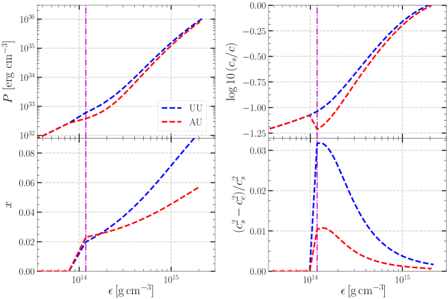
Figure 1: The left panels show the pressure $P$ (upper) and the proton fraction $x=n_{\mathrm{p}}/n$ (lower) versus the mass-energy density $\epsilon$ for representative EOS models AU and UU. The right panels show the relation between the adiabatic sound speed $c_{\mathrm{s}}$ and the fractional difference between $c_{\mathrm{s}}^{2}$ and $c_{\mathrm{e}}^{2}$ versus the mass-energy density $\epsilon$. The purple dashed line is the mass-energy density $\epsilon=0.07\,\rm fm^{-3}$.

In the upper left panel of Fig. 1, we show the EOS models AU and UU, which include below neutron-drip region [49] and the lower-density crustal region [50]. In the bottom left panel of Fig. 1, we show the relation between the proton fraction $x=n_{\mathrm{p}}/n$ and the mass-energy density $\epsilon$. One notices that the value of $x$ of model UU is larger than that of model AU. In the right panels of Fig. 1, we show the relation between the adiabatic sound speed $c_{\mathrm{s}}$ and the fractional difference between $c_{\mathrm{s}}^{2}$ and $c_{\mathrm{e}}^{2}$, as functions of the mass-energy density. Note that, in our work, we consider only $g$-mode of the NS core, so we set $c_{\mathrm{s}}^{2}=c_{\mathrm{e}}^{2}$ in the lower-density region. As mentioned in Sec. 4 of Lai [31] that $c_{\mathrm{s}}^{2}=c_{\mathrm{e}}^{2}$ in the crustal region indicates effectively suppressing the crustal $g$-mode while concentrating on the core $g$-mode.

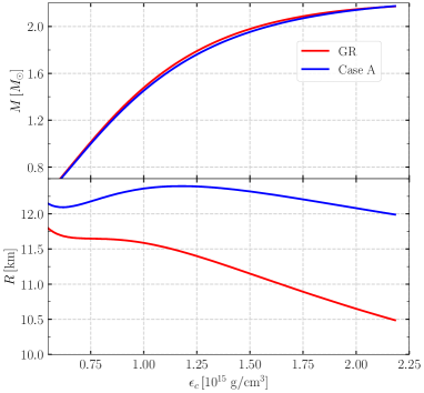
Figure 2: Mass and radius of model UU as a function of central density $\epsilon_{c}$. The Case A and GR lines represent the background equations calculated by the Case A and TOV schemes, respectively.

As shown in Fig. 2, the mass and radius of model UU are plotted against the central density $\epsilon_{c}$. The Case A and GR lines represent the background equations calculated by the Case A and TOV schemes, respectively (see Table 1). We can see that the masses computed in the Case A formulation can approximate well the GR solutions. The Case A formulation has absolute percentage differences $5$–$17\%$ for the radius of model UU. Note that the percentage difference of the stellar radii depends on the value of central density and the different EOS models. Detailed percentage differences of the stellar radii are illustrated in Appendix B of Tang and Lin [10].

The energy density profiles of the GR and Case A schemes with central density $\epsilon=2.0\times 10^{15}\rm g\,cm^{-3}$ for model UU is shown in Fig. 3. Compared with the GR solution, the Case A solution has a noticeable deviation only in the outer region of the surface. The total mass of the star is mainly determined by the high-density inner region. The above results may explain the fact that the total mass computed in the Case A formulation approximates well the GR solutions, though the radius has a large deviation.

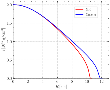
Figure 3: Comparison of the energy density profiles of the GR and Case A background solutions for model UU.

Note that the rest-mass density $\rho$ appears in the background and perturbation equations in N and N+lapse schemes; the total energy density $\epsilon$ and rest-mass density $\rho$ exhibit the background equations in Case A and Case A+lapse schemes, but the rest-mass density $\rho$ appears in the perturbation equations. To compare with the results of Lai [31], we use the energy density $\epsilon$ to obtain the mass-radius relation, as well as to solve perturbation equations. The difference between Case A and GR is apparent, though much smaller than the difference between Newtonian gravity and GR. Case A potential has captured some main effects from the full GR. As we will see, the perturbation results will be even closer to that of GR than the background results.

Lai [31] investigated $f$ and $g$ mode frequencies of EOS models AU and UU with a given mass $M=1.4\,M_{\odot}$. They found that the $f$-mode properties are very similar, due to the fact that the two EOSs have similar bulk properties ($V_{0}$) for the nuclear matter. However, the properties of the $g$-mode are very different from models AU and UU. From the bottom right panel of Fig. 1, we find that the value of $(c_{\mathrm{s}}^{2}-c_{\mathrm{e}}^{2})/c_{\mathrm{s}}^{2}$ is different with increase of the energy density. These differences reflect the sensitive dependence of $g$-mode on the nuclear matter’s symmetry energy ($V_{2}$).

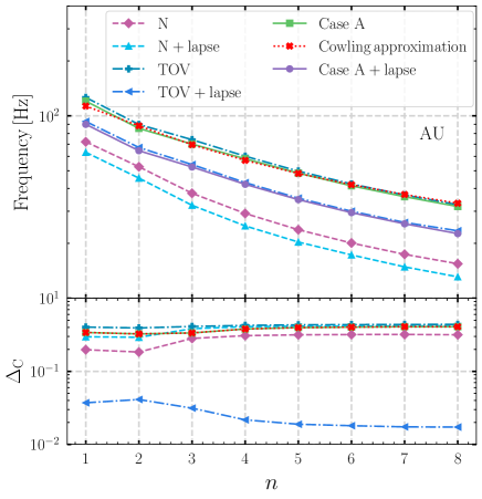
Figure 4: The $g$-mode frequencies for the EOS model AU, with a given mass $M=1.98\,M_{\odot}$. The upper panel shows the frequencies of the first eight quadrupolar ($\ell=2$) $g$-modes with different schemes. The lower panel shows the absolute fractional difference $\Delta_{\rm C}$ between our numerical results and the Case A+lapse scheme.

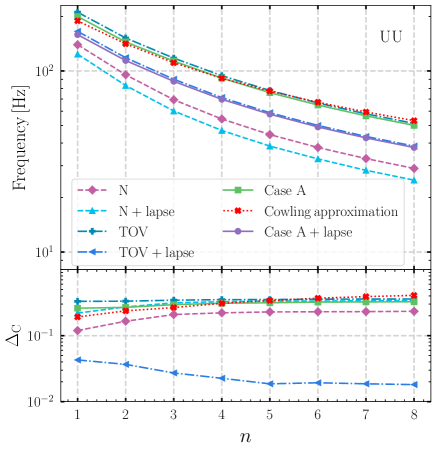
Figure 5: Same as Fig. 4, bur for the EOS model UU.

In our study, we extend calculations in Lai [31] by computing the $g$-mode. We use the stars with a fixed mass $M=1.98\,M_{\odot}$ as an example. In the upper panel of Fig. 4, we plot the frequencies of the first eight quadrupolar $g$-mode for the EOS AU. The results computed by all perturbation schemes are represented by different color lines in Fig. 4. The lower panel of Fig. 4 shows the absolute fraction difference $\Delta_{\rm C}$ defined by

$$\Delta_{\rm C}=\left\lvert\frac{f-f_{\text{Case A+lapse}}}{f_{\text{Case A+lapse}}}\right\rvert\,,$$ (54)

where $f$ is the frequency of $g$-mode obtained by our perturbation schemes in Table 1. According to the numerical results of non-radial oscillation ($f$-mode) in Tang and Lin [10], the Case A+lapse scheme can approximate to about a few percents for a given mass $M=1.4\,M_{\odot}$ in full GR. Hence, we use the results of Case A+lapse as the baseline in the case of the composition gradient. In particular, we found that the TOV+lapse scheme can give a good approximation to the $g$-mode frequencies to a few percent levels. Besides, the absolute percentage difference $\Delta_{\rm C}$ of the TOV+lapse scheme decreases with increasing nodes. We also plot the results of frequencies of $g$-mode and the absolute percentage difference $\Delta_{\rm C}$ for the EOS UU in Fig. 5. We seen similar properties of $g$-mode, as the EOS AU in Fig. 4.

III.2 Density discontinuity

In this subsection, we study the effect of discontinuities at high density on the oscillation spectrum of a NS. We consider a simple polytropic EOS of the form [21, 22, 24]

$$P=\left\{\begin{array}[]{rl}K\epsilon^{\gamma}\,,&\epsilon>\epsilon_{\rm{d}}+\Delta\epsilon\,,\\ \displaystyle{K\left(1+\frac{\Delta\epsilon}{\epsilon_{\rm{d}}}\right)^{\gamma}\epsilon^{\gamma}}\,,&\epsilon\leq\epsilon_{\rm{d}}\,,\end{array}\right.$$ (55)

where the discontinuity of amplitude $\Delta\epsilon$ is located at a mass-energy density $\epsilon_{\rm d}$. We study the properties of $g$-modes with density discontinuity using the pseudo-Newtonian gravity schemes in Table 1.

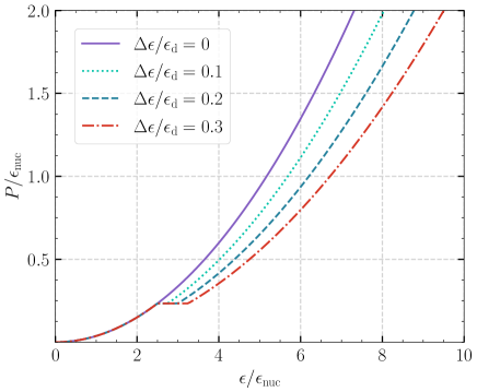
Figure 6: EOSs with density discontinuity, for different values of $\Delta\epsilon/\epsilon_{\rm{d}}$. The density and pressure are normalized by the standard nuclear density $\epsilon_{\rm nuc}=2.68\times 10^{14}\ \rm g\ cm^{-3}$.

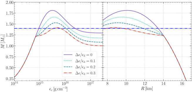
Figure 7: (Left) The relation between the mass of NSs and central density $\epsilon_{c}$ for different values of $\Delta\epsilon/\epsilon_{\rm{d}}$. (Right) Mass and radius relation of NSs with the same value of $\Delta\epsilon/\epsilon_{\rm{d}}$. The horizontal blue line shows the mass $M=1.4\,M_{\odot}$.

Now we have five parameters for a NS: the central density $\epsilon_{c}$, the discontinuity of amplitude $\Delta\epsilon$, the critical density $\epsilon_{\rm d}$, the polytropic index $\gamma$, and $K$. To compared with the results of non-radial oscillating relativistic stars in the full theory [i.e. without the relativistic Cowling approximation, 24], we adopt the same parameters as Miniutti et al. [24]: the polytropic index $\gamma=2$, $K=180\ \rm km^{2}$ for the NSs without discontinuity, and $K(1+\Delta\epsilon/\epsilon_{\rm{d}})^{2}=180\ \rm km^{2}$ for the case with a discontinuity. Some examples of this EOS are illustrated in Fig. 6.

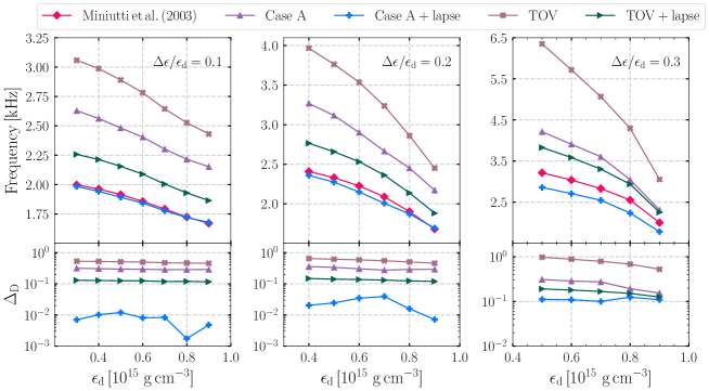
Figure 8: The top panels plot the frequency of the non-radial $f$-mode for different values of $\Delta\epsilon/\epsilon_{\rm{d}}$ versus the density $\epsilon_{\rm d}$ for the four perturbation schemes. The bottom panels show the absolute fractional difference $\Delta_{\rm D}$ between our numerical results and the results of Miniutti et al. [24]. We here consider stars with a fixed mass $M=1.4\,M_{\odot}$

.

Figure 9: Same as Fig. 8, but for the $g$-mode frequencies.

In performing the calculation, boundary conditions must be specified at the locations of the density discontinuities. Finn [21] analyzed the jump conditions of the perturbation variables with the Cowling approximation in Newtonian gravity. Since the density is discontinuous, the perturbation variables are discontinuous as well, and the differential equations (28–31) require jump conditions in the discontinuity density, denoted as [$\rho$]

$$[U]=0\,,$$ (56)

$$[\delta\tilde{P}]=g_{N}[\rho]U\,,$$ (57)

$$[\delta\tilde{\Phi}]=-4\pi[\rho]U\,,$$ (58)

$$[\Psi]=0\,.$$ (59)

To compare with the results of Miniutti et al. [24], we use the energy density $\epsilon$ to solve perturbation equations.

In the left panel of Fig. 7, we show the mass $M$ versus central density $\epsilon_{c}$ for each value of $\Delta\epsilon/\epsilon_{\rm{d}}$. As $\Delta\epsilon/\epsilon_{\rm{d}}$ gets larger, the maximum mass decreases, and the stable region $\mathrm{d}M/\rm d\epsilon_{c}>0$ becomes narrower and moves to a high-density region. In this work, we study only stable NS models with $\rm dM/\rm d\epsilon_{c}>0$. In our analysis, we fix the mass of a NS to $M=1.4\,M_{\odot}$ as an example. In the right panel of Fig. 7, we plot the mass-radius relation for NSs with and without density discontinuity. In both cases, we set the polytropic index $\gamma=2$. Comparing to the same EOS for $\epsilon<\epsilon_{\rm{d}}$, we adopt $K=180\ \rm km^{2}$ for the NS models without discontinuity, and $K(1+\Delta\epsilon/\epsilon_{\rm{d}})^{2}=180\ \rm km^{2}$ for the NS models with discontinuity. We find that the maximum mass is lower for the model with a discontinuity. Because the softening of EOS affected by the discontinuity. NSs with a discontinuity are more compact than those without discontinuity for a fixed mass.

Now we will focus on the $\ell=2$ non-radial oscillation modes. In particular, we consider the quadrupolar fundamental $f$-mode and gravity $g$-mode. The frequency versus density $\epsilon_{\rm{d}}$ for the fixed mass $M=1.4\,M_{\odot}$ is shown in the top panel of Fig. 8. The results computed by the four different perturbation schemes are represented by different color lines in Fig. 8. The GR curves in the upper panel correspond to the results of full perturbation theory in GR [24]. Additionally, the absolute fraction difference $\Delta_{\rm D}$ defined by

$$\Delta_{\rm D}=\left\lvert\frac{f-f_{\text{GR}}}{f_{\text{GR}}}\right\rvert\,,$$ (60)

is shown in the bottom panel of Fig. 8. The frequency of $f$-mode of the Case A+lapse scheme decreases with increasing density $\epsilon_{\rm d}$, which is similar to the GR results in trend. Again, the Case A+lapse scheme is quite accurate for the frequency of the $f$-mode. For the $\Delta\epsilon/\epsilon_{\rm{d}}=0.3$, the Case A+lapse scheme is not as good as that of the $\Delta\epsilon/\epsilon_{\rm{d}}=0.1,0.2$ cases, but it is still the best among the four perturbation schemes. Tang and Lin [10] calculated $f$-mode using Newtonian, Newtonian+lapse, Case A, and Case A+lapse schemes. They found that the Case A+lapse scheme performs much better and can reasonably approximate the $f$-mode frequency.

Figure 10: The top panels plot the frequency of the non-radial $f$-mode for different values of $\Delta\epsilon/\epsilon_{\rm{d}}$ versus the density $\epsilon_{\rm d}$ for the four perturbation schemes. The bottom panels show the absolute fractional difference $\Delta_{\rm D}$ between our numerical results and the results of Sotani et al. [23]. We here consider stars with a fixed mass $M=1.2\,M_{\odot}$

.

Figure 11: Same as Fig. 10, but for the $g$-mode frequencies.

Figure 12: The top panel plots the frequency of the non-radial $f$-mode with $\Delta\epsilon/\epsilon_{\rm{d}}=0.3$ versus the density $\epsilon_{\rm d}$ for the different perturbation schemes. The bottom panel shows the absolute fractional difference $\Delta_{\rm D}$ between our numerical results and the results of Miniutti et al. [24]. Here we consider stars with a fixed mass $M=1.4\,M_{\odot}$.

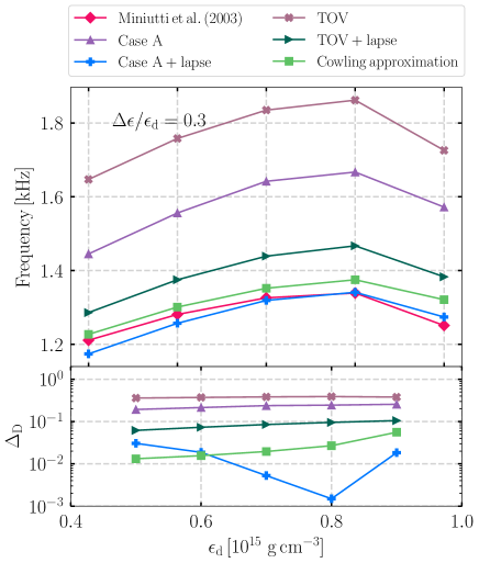
Figure 13: Same as Fig. 12, but for the $g$-mode frequencies.

In the top panel of Fig. 9, we show the frequency of $g$-mode as a function of the density $\epsilon_{\rm d}$ for the four schemes and the results of Miniutti et al. [24]. We also plot the results of $\Delta_{\rm D}$ for the four schemes at the bottom of Fig. 9. In particular, we find that the Case A+lapse scheme can approximate the $g$-mode frequency of GR reasonably well [24]. The percentage difference $\Delta_{\rm D}$ of $g$-mode of the Case A+lapse scheme decreases with increasing $\Delta\epsilon/\epsilon_{\rm{d}}$. The Case A+lapse scheme provides the best approximation to the frequencies of $f$ and $g$ modes. For the same central density and discontinuity density, the radius of density discontinuity $R_{\rm{d}}$ is larger than the radius $R$ of the Newtonian star. Hence, we ignore the N and N+lapse schemes of discontinuity $g$-mode in this work. Numerical results of the different schemes are given in Tables 3 and 4.

To prove that the pseudo-Newtonian treatments can approximate well the GR solutions, we also calculate the $f$ and $g$ modes of mass $M=1.2\,M_{\odot}$ for the different schemes. Detailed numerical results of the different schemes are given in Fig. 10, Fig. 11, as well as in Tables 5 and 6. We find that the pseudo-Newtonian gravity can accurately describe the oscillation of the relativistic NSs constructed from an EOS with a first-order phase transition.

For a given density $\epsilon_{\rm d}$ and $\Delta\epsilon/\epsilon_{\rm d}$, we show our numerical results for the frequencies of $f$ and $g$ modes with four schemes and the GR scheme, where the GR results were calculated by Miniutti et al. [24], Sotani et al. [23]. They integrated the equations describing the polar, non-radial perturbations of a non-rotating star as formulated by Lindblom and Detweiler [53] and Detweiler and Lindblom [54].

Finally, Sotani et al. [23] used the Cowling approximation to calculate the $f$ and $g$ modes and compared them to the results obtained from full GR. The results computed by the different perturbation schemes are represented by different colored lines in Fig. 12 and Fig. 13. We can see that the Case A+lapse scheme provides the best approximation to the frequency of $g$-mode when the central density increases.

Table 3: Comparison between the frequencies of $f$-mode (unit: Hz) of Miniutti et al. [24] and the different schemes in Table 1, with a given mass $M=1.4\,M_{\odot}$ and $\Gamma=2$ with different central densities. The polytropic coefficient $K$ is $K(1+\Delta\epsilon/\epsilon)^{2}=180\,\rm km^{2}$.

$\epsilon_{\rm d}\ (\rm g\,cm^{-3})$	$\Delta\epsilon/\epsilon_{\rm d}$	Miniutti et al. [24]	Case A	Case A+lapse	TOV	TOV+lapse
–	0.0	1666	2144	1673	2423	1863
$3\times 10^{14}$	0.1	1998	2629	1984	3058	2257
$4\times 10^{14}$	0.1	1962	2562	1942	2987	2213
$5\times 10^{14}$	0.1	1915	2482	1892	2890	2155
$6\times 10^{14}$	0.1	1857	2404	1842	2782	2089
$7\times 10^{14}$	0.1	1792	2302	1777	2644	2004
$8\times 10^{14}$	0.1	1723	2215	1720	2526	1929
$9\times 10^{14}$	0.1	1670	2152	1678	2431	1864
$4\times 10^{14}$	0.2	2408	3269	2359	3968	2765
$5\times 10^{14}$	0.2	2330	3117	2273	3764	2658
$6\times 10^{14}$	0.2	2226	2901	2149	3536	2532
$7\times 10^{14}$	0.2	2088	2665	2006	3238	2362
$8\times 10^{14}$	0.2	1901	2451	1871	2860	2137
$9\times 10^{14}$	0.2	1680	2171	1692	2451	1881
$5\times 10^{14}$	0.3	3216	4213	2859	6350	3829
$6\times 10^{14}$	0.3	3039	3909	2708	5718	3585
$7\times 10^{14}$	0.3	2831	3605	2547	5066	3305
$8\times 10^{14}$	0.3	2553	3044	2236	4298	2938
$9\times 10^{14}$	0.3	2002	2311	1783	3053	2254

Table 4: Same as Table 3, but for the $g$-mode frequencies.

$\epsilon_{\rm d}\ (\rm g\,cm^{-3})$	$\Delta\epsilon/\epsilon_{\rm d}$	Miniutti et al. [24]	Case A	Case A+lapse	TOV	TOV+lapse
–	0.0	–	–	–	–	–
$3\times 10^{14}$	0.1	504	571	500	604	523
$4\times 10^{14}$	0.1	567	660	570	695	596
$5\times 10^{14}$	0.1	613	730	624	766	651
$6\times 10^{14}$	0.1	644	786	665	820	690
$7\times 10^{14}$	0.1	659	828	692	855	712
$8\times 10^{14}$	0.1	658	858	708	874	720
$9\times 10^{14}$	0.1	641	876	713	876	712
$4\times 10^{14}$	0.2	840	987	834	1059	883
$5\times 10^{14}$	0.2	912	1093	916	1168	969
$6\times 10^{14}$	0.2	961	1173	976	1252	1032
$7\times 10^{14}$	0.2	987	1229	1016	1305	1070
$8\times 10^{14}$	0.2	979	1262	1034	1311	1071
$9\times 10^{14}$	0.2	906	1240	1009	1240	1010
$5\times 10^{14}$	0.3	1211	1445	1174	1647	1286
$6\times 10^{14}$	0.3	1281	1556	1257	1758	1375
$7\times 10^{14}$	0.3	1326	1642	1319	1835	1439
$8\times 10^{14}$	0.3	1339	1667	1341	1862	1467
$9\times 10^{14}$	0.3	1251	1572	1274	1726	1383

Table 5: Comparison between the frequencies of $f$-mode (unit: Hz) of Sotani et al. [23] and the different schemes, with a given mass $M=1.2\,M_{\odot}$ for different central densities.

$\epsilon_{\rm d}\ (\rm g\,cm^{-3})$	$\Delta\epsilon/\epsilon_{\rm d}$	Sotani et al. [23]	Case A	Case A+lapse	TOV	TOV+lapse
$8\times 10^{14}$	0.1	2575	3514	2574	4148	2952
$1.2\times 10^{15}$	0.1	2745	3792	2726	4542	3159
$1.6\times 10^{15}$	0.1	2818	3913	2788	4721	3249
$8\times 10^{14}$	0.2	2982	4212	2967	5112	3464
$1.2\times 10^{15}$	0.2	3230	4643	3180	5776	3774
$1.6\times 10^{15}$	0.2	3386	4914	3303	6231	3971
$8\times 10^{14}$	0.3	3588	5426	3565	6898	4267
$1.2\times 10^{15}$	0.3	4046	6440	3970	6647	4890

Table 6: Same as Table 5, but for the $g$-mode frequencies.

$\epsilon_{\rm d}\ (\rm g\,cm^{-3})$	$\Delta\epsilon/\epsilon_{\rm d}$	Sotani et al. [23]	Case A	Case A+lapse	TOV	TOV+lapse
$8\times 10^{14}$	0.1	727	856	730	901	761
$1.2\times 10^{15}$	0.1	871	1076	891	1134	931
$1.6\times 10^{15}$	0.1	963	1247	1004	1311	1048
$8\times 10^{14}$	0.2	1041	1234	1033	1318	1084
$1.2\times 10^{15}$	0.2	1271	1570	1277	1688	1349
$1.6\times 10^{15}$	0.2	1439	1847	1463	1994	1554
$8\times 10^{14}$	0.3	1272	1558	1260	1692	1329
$1.2\times 10^{15}$	0.3	1595	2021	1575	2228	1674

IV Conclusions

In light of new observations, oscillating modes of NSs are of particular interests to the physics and astrophysics communities in recent years. In this work, we have investigated the properties of the gravity $g$-mode for NSs in the framework of pseudo-Newtonian gravity. Tang and Lin [10] have investigated barotropic oscillations ($\Gamma_{1}=\gamma$ and the Schwarzschild discriminant $A=0$). We extended the work and have studied the $g$-mode of NSs with the same polytropic EOS model. We find that, the $g$-mode frequencies increase with increasing adiabatic index, which indicates that the buoyancy becomes much larger.

A deeper understanding of the oscillation of NSs, which could be associated with emitted gravitational waves, requires an analysis of both the state and composition of the NS matter. We considered the case of the composition gradient, and have extended calculations in Lai [31] to compute the $g$-mode. The value of $(c_{\mathrm{s}}^{2}-c_{\mathrm{e}}^{2})/c_{\mathrm{s}}^{2}$ is different when the energy density increases. In particular, these differences reflect the sensitive dependence of $g$-mode on the nuclear matter’s symmetry energy [$V_{2}$ in Eq. (39))]. Note that the tidal deformability of binary NSs appears to be related to the dominant oscillation frequency of the post-merger remnant [55]. The impact of thermal and rotational effects can provide simple arguments that help explain the result [56]. More recently, Andersson et al. [57] consider the dynamic tides of NSs to build the structure NSs in the framework of post-Newtonian gravity. We may expect using the pseudo-Newtonian gravity to study the resonant oscillations and tidal response in coalescing binary NSs in the future.

We considered a phase transition occurring in the inner core of NSs, which could be associated with a density discontinuity. Phase transition would produce a softening of EOSs, leading to more compact NSs. Using the different schemes, we have calculated the frequencies of $f$ and $g$ modes for the $\ell=2$ component. Compared to the results of GR [24, 23], the Case A+lapse scheme can approximate the $f$-mode frequency very well. The absolute percentage difference $\Delta_{\rm D}$ ranges from $0.01$ to $0.1$ percent. In particular, we find that the Case A+lapse scheme also can approximate the $g$-mode frequency of GR reasonably well [24, 23]. The percentage difference $\Delta_{\rm D}$ of $g$-mode of the Case A+lapse scheme decreases with increasing $\Delta\epsilon/\epsilon_{\rm{d}}$ in our model.

The existence of a possible hadron-quark phase transition in the central regions of NSs is associated with the appearance of $g$-mode, which is extremely important as they could signal the presence of a pure quark matter core in the center of NSs [58]. Our findings suggest that the pseudo-Newtonian gravity, with much less computational efforts than the full GR, can accurately study the oscillation of the relativistic NSs constructed from an EOS with a first-order phase transition. Observations of $g$-mode frequencies with density discontinuity may thus be interpreted as a possible hint of the first-order phase transition in the core of NSs. Lastly, our work also provides more confidence in using the pseudo-Newtonian gravity in the simulations of CCSNs, thus reducing the computational cost significantly.

McDermott et al. [13] investigated the non-radial oscillation of NSs using Cowling approximation and discussed the different damping mechanisms. Reisenegger and Goldreich [11] considered the $g$-mode induced by composition (proton-to-neutron ratio) gradient in the cores of NSs and discussed damping mechanisms. They also estimated damping rates for the core $g$-modes. Cutler et al. [59] assessed the accuracy of Cowling eigenfunctions and found that the relativistic Cowling approximation by McDermott et al. [12] accurately predicts frequencies and eigenfunctions. Chugunov and Gusakov [60] calculated the non-radial oscillations of superfluid non-rotating stars. An approximate decoupling of equations describing the oscillation modes of superfluid and normal fluid has been studied by Gusakov and Kantor [61]. Further, Gusakov et al. [62] developed an approximate method to determine the eigenfrequencies and eigenfunctions of an oscillating superfluid NS. In this work, we found that the $g$-mode frequencies in one of the pseudo-Newtonian treatments can approximate remarkably well the GR solutions than the relativistic Cowling approximation. Hence, we may conjecture that the eigenfunction and dissipation of the pseudo-Newtonian treatments are also more accurate than the relativistic Cowling approximation. Based on the approximate method of Gusakov et al. [62], one can calculate the eigenfunctions and the different damping mechanisms in future studies.