p-Adic Statistical Field Theory and Convolutional Deep Boltzmann Machines

Abstract

Understanding how deep learning architectures work is a central scientific problem. Recently, a correspondence between neural networks (NNs) and Euclidean quantum field theories (QFTs) has been proposed. This work investigates this correspondence in the framework of $p$-adic statistical field theories (SFTs) and neural networks (NNs). In this case, the fields are real-valued functions defined on an infinite regular rooted tree with valence $p$, a fixed prime number. This infinite tree provides the topology for a continuous deep Boltzmann machine (DBM), which is identified with a statistical field theory (SFT) on this infinite tree. In the $p$-adic framework, there is a natural method to discretize SFTs. Each discrete SFT corresponds to a Boltzmann machine (BM) with a tree-like topology. This method allows us to recover the standard DBMs and gives new convolutional DBMs. The new networks use $O(N)$ parameters while the classical ones use $O(N^{2})$ parameters.

1 Introduction

The deep neural networks have been successfully applied to various tasks, including self-driving cars, natural language processing, and visual recognition, among many others, [1]-[2]. There is consensus about the need of developing a theoretical framework to understand how deep learning architectures work. Recently, physicists have proposed the existence of a correspondence between neural networks (NNs) and quantum field theories (QFTs), more precisely statistical field theory (SFT), see [3]-[12], and the references therein. This correspondence takes different forms depending on the architecture of the networks involved.

In [12], the study of the above-mentioned correspondence was initiated in the framework of the non-Archimedean statistical field theory (SFT). In this case, the background space (the set of real numbers) is replaced by the set of $p$-adic numbers, where $p$ is a fixed prime number. The $p$-adics are organized in a tree-like structure; this feature facilitates the description of hierarchical architectures. In [12], a $p$-adic version of the convolutional deep Boltzmann machines is introduced where only binary data is considered and with no implementation. By adapting the mathematical techniques introduced by Le Roux and Benigio in [13], the author shows that these machines are universal approximators for binary data tasks.

In this article, we continue discussing the correspondence between STFs and NNs, in the $p$-adic framework. Compare with [12] here we consider more general architectures and data types. We note that dealing with general data is challenging both in theory and implementation practice. We argue that $p$-adic analysis still provides the right framework to understand the dynamics of NNs with large tree-like hierarchical architectures. In our approach, a NN corresponds to the discretization of a $p$-adic STF. The discretization process is carried out in a rigorous and general way. Moreover, such discretization allows us to obtain many recently developed deep BM. For instance, the NNs constructed in [5] are a particular case of the ones introduced here. We also discuss the implementation of a class of $p$-adic convolutional networks and obtain desired results on a feature detection task based on hand-writing images of decimal digits.

The main novelty of our $p$-adic convolutional DBMs is that they use significantly fewer parameters than the conventional ones. A detailed discussion is given in Section 6. We note that the connections between $p$-adic numbers and neural networks have been considered before. Neural networks whose states are $p$-adic numbers were studied in [14, 15]. These models are completely different from the ones considered here. These ideas have been used to develop non-Archimedean models of brain activity and mental processes [16]. In [17, 18], p-adic versions of the cellular neural networks were studied. These models involved abstract evolution equations.

2 $p$-Adic Numbers

In this section, we introduce basic concepts for the $p$-adic numbers. For more detailed information, refer Section 7 (Appendix A).

From now on, $p$ denotes a fixed prime number. Any non-zero $p-$adic number $x$ has a unique expansion of the form

$$x=x_{-k}p^{-k}+x_{-k+1}p^{-k+1}+\ldots+x_{0}+x_{1}p+\ldots,\text{ }$$

with $x_{-k}\neq 0$, where $k$ is an integer, and the $x_{j}$s  are numbers from the set $\left\{0,1,\ldots,p-1\right\}$. The set of all possible numbers of such form constitutes the field of $p$-adic numbers $\mathbb{Q}_{p}$. There are natural field operations, sum, and multiplication, on $p$-adic numbers, see, e.g., [36]. There is also a natural norm in $\mathbb{Q}_{p}$ defined as $\left|x\right|_{p}=p^{k}$ where $k$ depends on $x$, for a nonzero $p$-adic number $x$.

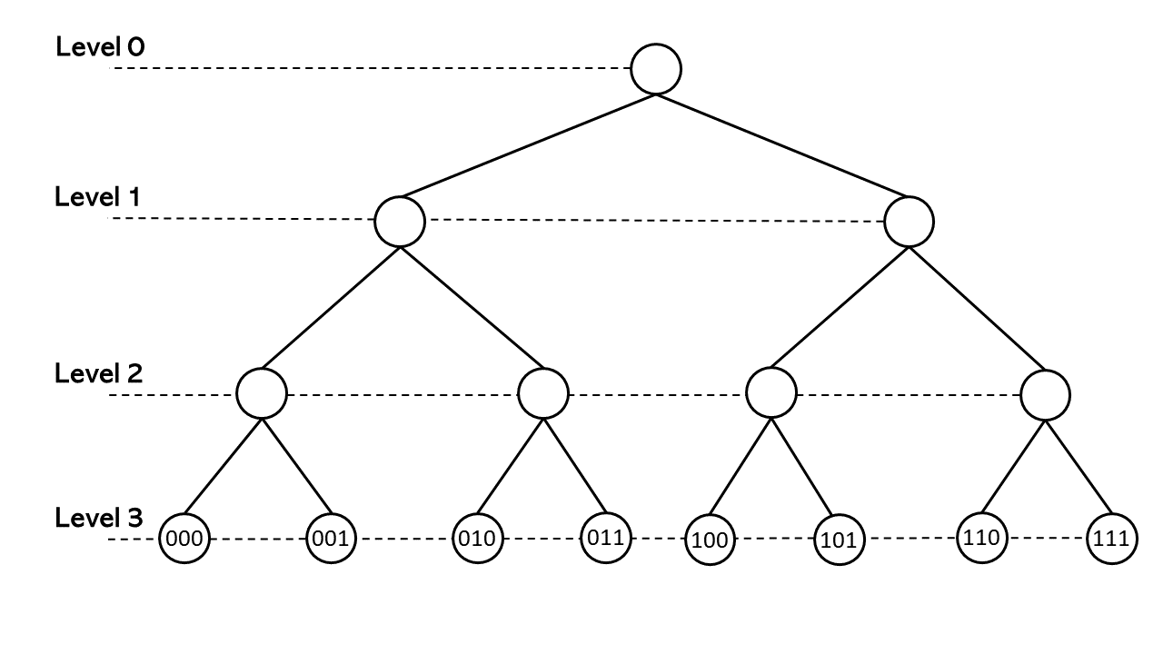
Figure 1: The rooted tree associated with the group $\mathbb{Z}_{2}/2^{3}\mathbb{Z}_{2}$. The elements of $\mathbb{Z}_{2}/2^{3}\mathbb{Z}_{2}$ have the form $i=i_{0}+i_{1}2+i_{2}2^{2}$,$\;i_{0}$, $i_{1}$, $i_{2}\in\{0,1\}$. The distance satisfies $-\log_{2}\left|i-j\right|_{2}=$level of the first common ancestor of $i$, $j$.

The field of $p$-adic numbers with the distance induced by $\left|\cdot\right|_{p}$ is a complete ultrametric space. The ultrametric property refers to the fact that $\left|x-y\right|_{p}\leq\max\left\{\left|x-z\right|_{p},\left|z-y\right|_{p}\right\}$ for any $x$, $y$, $z$ in $\mathbb{Q}_{p}$. In this article, we work with $p$-adic integers, which $p$-adic numbers satisfying $-k\geq 0$. All such $p$-adic integers constitute the unit ball $\mathbb{Z}_{p}$. The unit ball is closed under addition and multiplication, so it is a commutative ring. Along this article, we work mainly with locally constant functions supported in the unit ball, i.e., with functions of type $\varphi:\mathbb{Z}_{p}\rightarrow\mathbb{R}$, such that $\varphi\left(a+x\right)=\varphi\left(a\right)$ for all $x$ in $\mathbb{Z}_{p}$. The simplest example of such function is the chararcterisstic function $1_{\mathbb{Z}_{p}}\left(x\right)$ of the unit ball $\mathbb{Z}_{p}$: $1_{\mathbb{Z}_{p}}\left(x\right)=1$ if $\left|x\right|_{p}\leq 1$, otherwise $1_{\mathbb{Z}_{p}}\left(x\right)=0$. To check that $1_{\mathbb{Z}_{p}}\left(a+x\right)=1_{\mathbb{Z}_{p}}\left(a\right)$, we use that $\mathbb{Z}_{p}$ is closed under addition. If $\left|x\right|_{p}\leq p^{-l}$, where the integer $l$ is fixed and independent of $a$. We denote by $\mathcal{D}(\mathbb{Z}_{p})$ the real vector space of test functions supported in the unit ball. There is a natural integration theory so that $\int_{\mathbb{Z}_{p}}\varphi\left(x\right)dx$ gives a well-defined real number. The measure $dx$ is the so-called Haar measure of $\mathbb{Q}_{p}$. Further details are given in Section 7.3.

Since the $p$-adic numbers are infinite series, any computational implementation involving these numbers requires a truncation process: $x\longmapsto x_{0}+x_{1}p+\ldots+x_{l-1}p^{l-1}$, $l\geq 1$. The set of all truncated integers mod $p^{l}$ is denote as $G_{l}=\mathbb{Z}_{p}/p^{l}\mathbb{Z}_{p}$. This set can be represented as a rooted tree with $l$ levels; see Figure 1.

The unit ball $\mathbb{Z}_{p}$ is an infinite rooted tree with fractal structure; see Figure 2. Section 7 (Appendix A) provides review of the basic aspects of the $p$-adic analysis required here. We note that the word ‘field’ will be used here in two different contexts throughout the article. In a mathematical context, we refer to algebraic fields; in a physical context, we refer to Euclidean quantum fields.

3 Non-Archimedean $\left\{\boldsymbol{v},\boldsymbol{h}\right\}^{4}$-statistical field theories

We fix $a\left(x\right)$, $b(x)$, $c(x)$, $d(x)\in\mathcal{D}(\mathbb{Z}_{p})$, $e\in\mathbb{R}$, and an integrable function $w\left(x\right):\mathbb{Z}_{p}\rightarrow\mathbb{R}$ . A $p$-adic continuous Boltzmann machine (or a $p$-adic continuous BM) is a statistical field theory involving two scalars fields $\boldsymbol{v}$, $\boldsymbol{h}$. The function $\boldsymbol{v}(x)\in\mathcal{D}(\mathbb{Z}_{p})$ is called the visible field and the function $\boldsymbol{h}(x)\in\mathcal{D}(\mathbb{Z}_{p})$ is called the hidden field. We assume that the field $\left\{\boldsymbol{v},\boldsymbol{h}\right\}$ performs thermal fluctuations and that the expectation value of the field is zero.

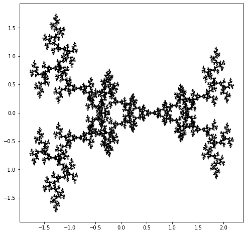
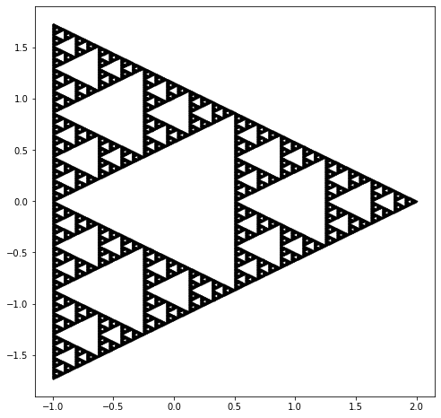
Figure 2: Based upon [37], we construct an embedding $\mathfrak{f}:\mathbb{Z}_{p}\rightarrow\mathbb{R}^{2}$. The figure shows the images of $\mathfrak{f}(\mathbb{Z}_{2})$ and $\mathfrak{f}(\mathbb{Z}_{3})$. This computation requires a truncation of the $p$-adic integers. We use $\mathbb{Z}_{2}/2^{14}\mathbb{Z}_{2}$ and $\mathbb{Z}_{3}/3^{10}\mathbb{Z}_{3}$, respectively.

The size of the fluctuations is controlled by an energy functional of the form

$$E(\boldsymbol{v},\boldsymbol{h};\boldsymbol{\theta}):=E(\boldsymbol{v},\boldsymbol{h})=E_{0}\left(\boldsymbol{v},\boldsymbol{h}\right)+E_{\text{int}}\left(\boldsymbol{v},\boldsymbol{h}\right),$$

where $\boldsymbol{\theta}=\left(w,a,b,c,d,e\right)$. The first term

$$E_{0}\left(\boldsymbol{v},\boldsymbol{h}\right)=-{\displaystyle\int\limits_{\mathbb{Z}_{p}}}a(x)\boldsymbol{v}\left(x\right)dx-{\displaystyle\int\limits_{\mathbb{Z}_{p}}}b(x)\boldsymbol{h}\left(x\right)dx+\frac{e}{2}{\displaystyle\int\limits_{\mathbb{Z}_{p}}}\boldsymbol{v}^{2}\left(x\right)dx+\frac{e}{2}{\displaystyle\int\limits_{\mathbb{Z}_{p}}}\boldsymbol{h}^{2}\left(x\right)dx$$

is an analogue of the free-field energy. The second term

$$E_{\text{int}}\left(\boldsymbol{v},\boldsymbol{h}\right)=-{\displaystyle\iint\limits_{\mathbb{Z}_{p}\times\mathbb{Z}_{p}}}\boldsymbol{h}\left(y\right)w\left(x-y\right)\boldsymbol{v}\left(x\right)dxdy+{\displaystyle\int\limits_{\mathbb{Z}_{p}}}c(x)\boldsymbol{v}^{4}\left(x\right)dx+{\displaystyle\int\limits_{\mathbb{Z}_{p}}}d(x)\boldsymbol{h}^{4}\left(x\right)dx$$

is an analogue of the interaction energy. The results presented in this section are valid for more general functionals in which the first term in $E_{\text{int}}(\boldsymbol{v},\boldsymbol{h})$ is replaced by

$${\displaystyle\iint\limits_{\mathbb{Z}_{p}\times\mathbb{Z}_{p}}}\boldsymbol{h}\left(y\right)w\left(x,y\right)\boldsymbol{v}\left(x\right)dxdy.$$

The motivation behind the definition of the energy functionals $E(\boldsymbol{v},\boldsymbol{h})$ is that the discretizations of these functionals give the energy functionals considered in [5], [13], [38]-[39].

All the thermodynamic properties of the system are described by the partition function of the fluctuating fields, which is defined as

$$Z^{\text{phys}}(\boldsymbol{\theta})={\displaystyle\int}d\boldsymbol{v}d\boldsymbol{h}\text{ }e^{-\frac{E(\boldsymbol{v},\boldsymbol{h})}{K_{B}T}},$$

where $K_{B}$ is the Boltzmann constant and $T$ is the temperature constant. We normalize in such a way that $K_{B}T=1$. The measure $d\boldsymbol{v}d\boldsymbol{h}$ is ill-defined. However, it is expected that such measure can be defined rigorously by a limit process. The statistical field theory corresponding to the energy functional $E(\boldsymbol{v},\boldsymbol{h};\boldsymbol{\theta})$ is defined as the probability measure

$$\boldsymbol{P}^{\text{phys}}(\boldsymbol{v},\boldsymbol{h};\boldsymbol{\theta})=d\boldsymbol{v}d\boldsymbol{h}\frac{\exp\left(-E(\boldsymbol{v},\boldsymbol{h})\right)}{Z^{\text{phys}}},$$

on the space $\mathcal{D}(\mathbb{Z}_{p})\times\mathcal{D}(\mathbb{Z}_{p})$.

The information about the local properties of the system is contained in the correlation functions $G_{\mathbb{I},\mathbb{K}}^{\left(n\right)}\left(x_{1},\ldots,x_{n}\right)$ of the field $\left\{\boldsymbol{v},\boldsymbol{h}\right\}$: for $n\geq 1$, and two disjoint subsets $\mathbb{I}$, $\mathbb{K}\subset\left\{1,2,\ldots,n\right\}$, with $\mathbb{I}{\textstyle\coprod}\mathbb{K}=\left\{1,2,\ldots,n\right\}$, where ${\textstyle\coprod}$ is the disjoint union, we set

$$G_{\mathbb{I},\mathbb{K}}^{\left(n\right)}\left(x_{1},\ldots,x_{n}\right)=\left\langle{\displaystyle\prod\limits_{i\in\mathbb{I}}}\boldsymbol{v}\left(x_{i}\right)\text{ }{\displaystyle\prod\limits_{j\in\mathbb{K}}}\boldsymbol{h}\left(x_{j}\right)\right\rangle$$

$$:=\frac{1}{Z^{\text{phys}}}{\displaystyle\int}d\boldsymbol{v}d\boldsymbol{h}\text{ }{\displaystyle\prod\limits_{i\in\mathbb{I}}}\boldsymbol{v}\left(x_{i}\right)\text{ }{\displaystyle\prod\limits_{j\in\mathbb{K}}}\boldsymbol{h}\left(x_{j}\right)\text{ }e^{-E(\boldsymbol{v},\boldsymbol{h})}.$$

These functions are also called the $n$-point Green functions.

To study these functions, one introduces two auxiliary external fields $J_{0}(x),$ $J_{1}(x)\in\mathcal{D}(\mathbb{Z}_{p})$ called currents, and adds to the energy functional $E$ as a linear interaction energy of these currents with the field $\left\{\boldsymbol{v},\boldsymbol{h}\right\}$,

$$E_{\text{source}}(\boldsymbol{v},\boldsymbol{h},J_{0},J_{1})=-{\displaystyle\int\limits_{\mathbb{Z}_{p}}}J_{0}(x)\boldsymbol{v}\left(x\right)dx-{\displaystyle\int\limits_{\mathbb{Z}_{p}}}J_{1}(x)\boldsymbol{h}\left(x\right)dx,$$

now the energy functional is $E(\boldsymbol{v},\boldsymbol{h},J_{0},J_{1})=E\left(\boldsymbol{v},\boldsymbol{h}\right)+E_{\text{source}}(\boldsymbol{v},\boldsymbol{h},J_{0},J_{1})$. The partition function formed with this energy is

$$Z(J_{0},J_{1})=\frac{1}{Z_{0}^{\text{phys}}}{\displaystyle\int}d\boldsymbol{v}d\boldsymbol{h}\text{ }e^{-E(\boldsymbol{v},\boldsymbol{h},J_{0},J_{1})},$$

where

$$Z_{0}^{\text{phys}}={\displaystyle\int}d\boldsymbol{v}d\boldsymbol{h}\text{ }e^{-E_{0}(\boldsymbol{v},\boldsymbol{h})}.$$

The functional derivatives of $Z(J_{0},J_{1})$ with respect to $J_{0}(x)$, $J_{1}(x)$ evaluated at $J_{0}=0$, $J_{1}=0$ give the correlation functions of the system:

$$G_{\mathbb{I},\mathbb{K}}^{\left(n\right)}\left(x_{1},\ldots,x_{n}\right)=\frac{1}{Z}\left[{\textstyle\prod\limits_{i\in\mathbb{I}}}\frac{\delta}{\delta J_{0}\left(x_{i}\right)}\text{ }{\textstyle\prod\limits_{j\in\mathbb{K}}}\frac{\delta}{\delta J_{1}\left(x_{j}\right)}Z(J_{0},J_{1})\right]_{\begin{subarray}{c}J_{0}=0\\ J_{1}=0\end{subarray}},$$

where $Z=\frac{Z^{\text{phys}}}{Z_{0}^{\text{phys}}}$. The functional $Z(J_{0},J_{1})$ is called the generating functional of the theory.

The description of the $\left\{\boldsymbol{v},\boldsymbol{h}\right\}^{4}$-SFTs presented above is based in the classical version of these theories [40]-[41]. In [31], a mathematically rigorous formulation of $\phi^{4}$-SFTs is presented, the fields are functions from $\mathbb{Q}_{p}^{N}$ into $\mathbb{R}$, with $N$ arbitrary. We expect that this theory can be extended to the $\left\{\boldsymbol{v},\boldsymbol{h}\right\}^{4}$-SFTs presented here.

4 Discrete SFTs and $p$-adic discrete Boltzmann machines

A central difference between the $p$-adic STFs and the classical ones is that in the $p$-adic case, the discretization process can be carried out in an easy rigorous way. More specifically, the discretization of a $p$-adic SFT is constructed by restricting the energy functional $E(\boldsymbol{v},\boldsymbol{h};\boldsymbol{\theta})$ to a finite dimensional vector subspace $\mathcal{D}^{l}(\mathbb{Z}_{p})$ of the space of test functions $\mathcal{D}(\mathbb{Z}_{p})$. The test functions in $\mathcal{D}^{l}(\mathbb{Z}_{p})$ have the form

$$\varphi\left(x\right)={\textstyle\sum\limits_{i\in G_{l}}}\varphi\left(i\right)\Omega\left(p^{l}\left|x-i\right|_{p}\right),\quad\varphi\left(i\right)\in\mathbb{R},$$

where $i\boldsymbol{=}i_{0}+i_{1}p+\ldots+i_{l-1}p^{l-1}\in G_{l}=\mathbb{Z}_{p}/p^{l}\mathbb{Z}_{p}$, $l\geq 1$, and $\Omega\left(p^{l}\left|x-i\right|_{p}\right)$ is the characteristic function of the ball $B_{-l}(i)$. Here, it is important to notice that $G_{l}$ is a finite, Abelian, additive group. In the $p$-adic world, the discrete functions are a particular case of the $p$-adic continuous functions, more precisely, $\mathcal{D}(\mathbb{Z}_{p})=\cup_{l\in\mathbb{N}}\mathcal{D}^{l}(\mathbb{Z}_{p})$ and $\mathcal{D}^{l}(\mathbb{Z}_{p})\subset$ $\mathcal{D}^{l+1}(\mathbb{Z}_{p})$. There is no Archimedean counterpart of this result.

By taking $\boldsymbol{v},\boldsymbol{h}\in\mathcal{D}^{l}(\mathbb{Z}_{p})$ and $l$ sufficiently large, the restriction $E_{l}\left(\boldsymbol{v},\boldsymbol{h};\boldsymbol{\theta}\right)$ of the energy functional $E(\boldsymbol{v},\boldsymbol{h};\boldsymbol{\theta})$ to $\mathcal{D}^{l}(\mathbb{Z}_{p})$ has the form

$$E_{l}\left(\boldsymbol{v},\boldsymbol{h};\boldsymbol{\theta}\right)=-{\displaystyle\sum\limits_{j\in G_{l}}}{\displaystyle\sum\limits_{k\in G_{l}}}w_{k}v_{j+k}h_{j}-{\displaystyle\sum\limits_{j\in G_{l}}}a_{j}v_{j}-{\displaystyle\sum\limits_{j\in G_{l}}}b_{j}h_{j}+\frac{e}{2}{\displaystyle\sum\limits_{j\in G_{l}^{N}}}v_{j}^{2}+\frac{e}{2}{\displaystyle\sum\limits_{j\in G_{l}}}h_{j}^{2}$$ (1)

$$+{\displaystyle\sum\limits_{j\in G_{l}}}c_{j}v_{j}^{4}+{\displaystyle\sum\limits_{j\in G_{l}}}d_{j}h_{j}^{4}\text{.}$$

We refer Section 8 (Appendix B) for further details of this calculation. From now on, we refer eq. 1 as the energy functional for a discrete $\left\{\boldsymbol{v},\boldsymbol{h}\right\}^{4}$-STF.

In the general case, $E_{l}\left(\boldsymbol{v},\boldsymbol{h};\boldsymbol{\theta}\right)$ is a $p$-adic analogue of the $\left\{\boldsymbol{v},\boldsymbol{h}\right\}^{4}$ neural networks introduced in [5]. In this article, each hidden state $h_{j}$ and visible state $v_{i}$ are interacted through a weight $w_{ij}$. Therefore, requires the number of $G_{l}^{2}$ for weights $w$, whereas our counterpart requires only $G_{l}$. See Section 6, for further discussion.

We now attach to the discrete energy functional a $p$-adic discrete BM. For any visible and hidden states, $\boldsymbol{v}=\left[v_{i}\right]_{i\in G_{l}}$ and  $\boldsymbol{h}=\left[h_{i}\right]_{i\in G_{l}}$, the Boltzmann probability distribution attached to $E_{l}\left(\boldsymbol{v},\boldsymbol{h};\boldsymbol{\theta}\right)$ is given by

$$\boldsymbol{P}_{l}(\boldsymbol{v},\boldsymbol{h};\boldsymbol{\theta})=\frac{\exp\left(-E_{l}\left(\boldsymbol{v},\boldsymbol{h};\boldsymbol{\theta}\right)\right)}{{\sum\limits_{\boldsymbol{v},\boldsymbol{h}}}\exp\left(-E_{l}\left(\boldsymbol{v},\boldsymbol{h};\boldsymbol{\theta}\right)\right)}.$$

When there is no risk of confusion, we will omit $\boldsymbol{\theta}$ in the notations. When $c_{j}=d_{j}=0$ for all $j\in G_{l}$, the energy functional $E_{l}\left(\boldsymbol{v},\boldsymbol{h};\boldsymbol{\theta}\right)$ corresponds to a $p-$adic analogue of the convolutional deep belief networks studied in [38].

We note that the energy functional $E_{l}$ has translational symmetry, i.e., $E_{l}$ is invariant under the transformations $j\rightarrow j+j_{0}$, $k\rightarrow k+k_{0}$, for any $j_{0}$, $k_{0}\in G_{l}$. This transformation is well-defined since $G_{l}$ is an additive group. In the case of applications to image processing, the group property also implies that the convolution operation does not alter image dimensions. The convolutional $p$-adic discrete BMs introduced here are a specific type of deep Boltzmann machines (DBMs) (also called deep belief networks DBNs).

5 Experimental Results

We implement a $p$-adic discrete Boltzmann machine for processing binary images, then $\boldsymbol{v},\boldsymbol{h}:\mathbb{Z}_{p}\rightarrow\left\{0,1\right\}\subset\mathbb{R}$, in this case, we use the following energy functional:

$$E_{l}\left(\boldsymbol{v},\boldsymbol{h};\theta\right)=-{\sum\limits_{j\in G_{l}}}{\sum\limits_{\begin{subarray}{c}k\in G_{l}\\ |k|_{p}\leq p^{-N}\end{subarray}}}w_{k}v_{j+k}h_{j}-{\sum\limits_{j\in G_{l}}}a_{j}v_{j}-{\sum\limits_{j\in G_{l}}}b_{j}h_{j}\text{,}$$

for some natural number $0\leq N\leq l$. Note that, comparing to Equation 1, the quadratic and biquadratic terms are omitted since they do not play any role in the case in which $\boldsymbol{v},\boldsymbol{h}$ are binary variables. The condition $N\leq l$ implies that the convolution operation is restricted to a small neighborhood of radius $p^{-N}$ for each pixel. The condition $N=0$ means that the convolution involves all the points in the image.

Our numerical experiment is based on the MNIST dataset, where each image is considered as a sample of the visible state. Our first task is to train the network to maximize the log-likelihood of the visible states. We choose $p=3$ and $l=6$ since image dimension is $3^{3}\times 3^{3}$. In general, $p$ and $l$ depend on the size of the images to be processed. Typically $p$ is chosen as a small prime number, e.g., $2$ or $3$.

To tune the parameters $a_{j}$, $b_{j}$, $w_{j}$, $j\in G_{6}$ of the network, we first transform each image $I$ into a test function $\text{Test}\left(I\right)\in\mathcal{D}^{6}(\mathbb{Z}_{3})$. The test function $\text{Test}(I)$ is defined in terms of the tree structure of $G_{6}$ in the following way: we define $I$ as the root of the tree. Later we divide $I$ into three horizontal even slices (sub-images). These sub-images are the vertices level $1$, and they are the children of $I$. Each sub-image $I_{j}$ at level $1$ is then divided vertically into $3$ sub-images; these are the children of the $I_{j}$. All the $3^{2}$ new sub-images correspond to the vertices at level $2$. We repeat this process until reaching level $6$. At level $6$, each vertex corresponds to a pixel, and we denote by value $I_{i}$ for $i\in G_{6}$. Then $\text{Test}(I)$ is defined as $\sum_{i\in G_{6}}I_{i}\Omega(3^{6}|x-i|_{3})$. See Figure 3 for the construction of the tree corresponding to a $3^{2}\times 3^{2}$ image. Figure 4 shows the graph of a test function corresponding to an image from the MNIST data set. For further details, the reader may consult the Appendix in [18].

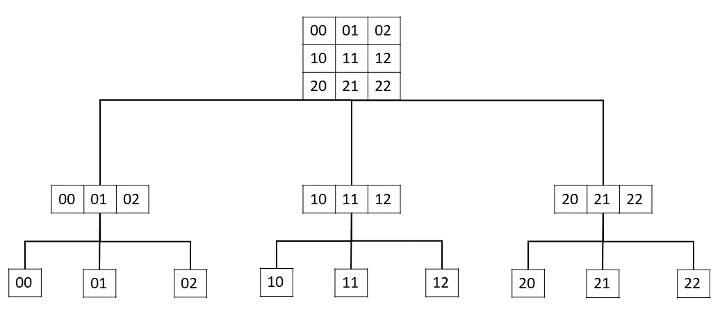
Figure 3: The construction of the tree corresponding to a $3\times 3$ image.

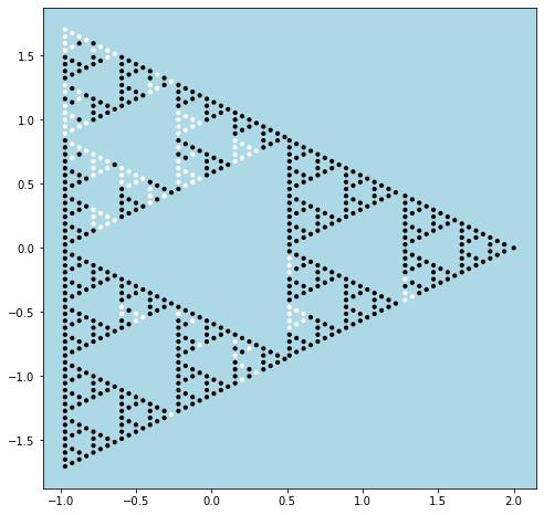
Figure 4: The processing of date using $p$-adic networks requires the transformation of the actual data to its $p$-adic form. The left image shows a visualization of the test function corresponding to right image. The visualization uses the embedding $\mathfrak{f}:\mathbb{Z}_{p}\rightarrow\mathbb{R}^{2}$ showed in Figure 2.

We note that in a $p$-adic discrete deep RBM, the visible and hidden states are functions on a finite tree. Only the vertices at the top level, which are marked as orange and blue balls are allowed to have states. See Figure 5 for the case $p=2,l=2$. The remaining trees’ vertices (see the black dots in Figure 5) only codify the hierarchical relation between states. The visible and hidden vertices connected by the same type of lines share the same weight $w$.

We adapted the contrastive divergence learning method to the $p$-adic framework, [48]. The technical details are presented in Section 9.2. We implement two different types of networks. In the first type, the function $w_{k}$ is supported in the entire tree $G_{6}$; in the second type, the function $w_{k}$ is supported in a proper subset of the tree $G_{6}$. We use the full MNIST hadwritten digits, without considering labels, to train a six layer $3$-adic feature detector. The results are show in Figure 6.

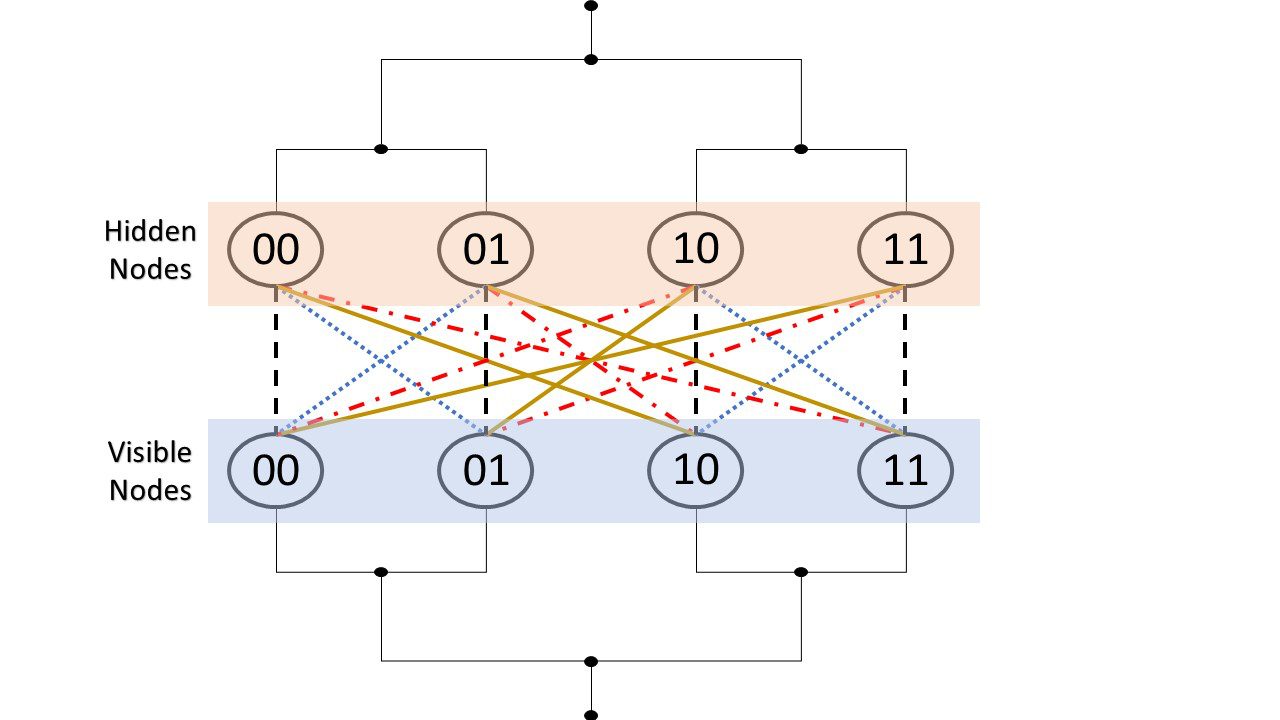
Figure 5: A p-adic RBM for $p=2,l=2$

After the processing by the network ends, it is necessary to transform the test function into an image.

6 Conclusions

The standard RBMs [48] and the $\phi^{4}$- neural networks introduced in [5] are particular classes of $p$-adic discrete BMs. Indeed, if $w(x,y)$ is a test function and the interaction between the visible and hidden field has the form $-{\textstyle\iint\nolimits_{\mathbb{Z}_{p}\times\mathbb{Z}_{p}}}\boldsymbol{h}\left(y\right)w\left(x,y\right)\boldsymbol{v}\left(x\right)dxdy$, then in the corresponding discrete energy functional, after a suitable rescaling of the weights $w_{k,j}$, the interaction of the visible and hidden states takes the form $-\sum_{j\in G_{l}}\sum_{k\in G_{l}}w_{k,j}v_{k}h_{j}$. Here $\left[w_{k,j}\right]$ is an ordinary matrix, which means that its entries $w_{k,j}$ do not depend on the algebraic structure of $G_{l}$ neither on its topology.

In the case in which the interaction between the visible and hidden field has the form $-{\textstyle\iint\nolimits_{\mathbb{Z}_{p}\times\mathbb{Z}_{p}}}\boldsymbol{h}\left(y\right)w\left(x-y\right)\boldsymbol{v}\left(x\right)dxdy$, then corresponding discrete energy functional depends on the group structure of $G_{l}$, and the corresponding neural network is a particular case of a DBM, see Figure 5.

The condition $l\geq l_{0}$, for some constant $l_{0}$, means that a $p$-adic discrete BM admits copies arbitratly large, this is a consequence of the fact of $p$-adic numbers has a tree-like structure. We expect that for $l$ sufficiently large the statistical properties of the network can be studied using a $p$-adic continuous SFT.

Our numerical experiments show that $p$-adic discrete convolutional deep BMs alone can be used to process real data, this opens the possibility of using these networks as layers in specialized NNs.

In [12] the first author conjectured that the limit

$$\frac{e^{-E(\boldsymbol{v},\boldsymbol{h})}}{Z^{\text{phys}}}d\boldsymbol{v}d\boldsymbol{h}=\lim_{l\rightarrow\infty}\boldsymbol{P}_{l}(\boldsymbol{v},\boldsymbol{h})\text{ }d^{\#G_{l}}\boldsymbol{v}\text{ }d^{\#G_{l}}\boldsymbol{h}$$ (2)

exists in some sense, here $d^{\#G_{l}}\boldsymbol{x}$ denotes the Lebesgue measure of $\mathbb{R}^{\#G_{l}}$. Then the correlation between the network activity in different regions of the underlaying tree $G_{l}$ can be understood by computing the correlations functions of the corresponding continuous SFT.

For practical applications the NNs should be discrete entities. This type of NNs naturally correspond with discrete SFTs. To use Euclidean QFT to study NNs, it is convenient to have continuous versions of these networks. Thus, a clear way of passing between discrete STFs to continuous ones is required. The existence of the limit 2 is a very difficult problem in classical QFT. In [31] the existence of this limit was established for $p$-adic $\phi^{4}$- theories involving one scalar field, we expect that these techniques can be extended to the case QFTs considered here.

It is widely accepted in the artificial intelligence community that the probability distributions $\boldsymbol{P}_{l}(\boldsymbol{v},\boldsymbol{h})$ should approximate any finite probability distribution very well, which means that the corresponding NNs are universal approximators. We argue that this property is connected with the topology and the structure of the NNs, and that the problem of designing good architectures for NNs is out of the scope of QFT. We expect that QFT techniques will be useful to understand the qualitative behavior of large NNs, which can be well-approximated as ‘continuos’ NNs.

The study of the correspondence between $p$-adic Euclidean QFTs and NNs is just starting. We envision that the next step is to develop perturbative calculations of the correlation functions via Feynman diagrams, to study connections with Ginzburg–Landau theory, and to develop practical applications of the $p$-adic convolutional BMs.

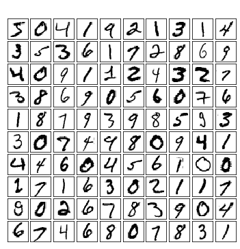
(a)

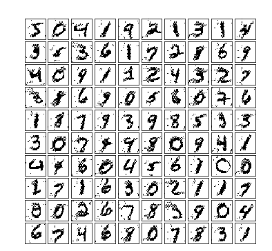
(b)

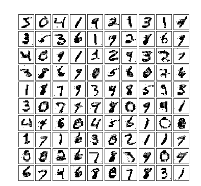
(c)

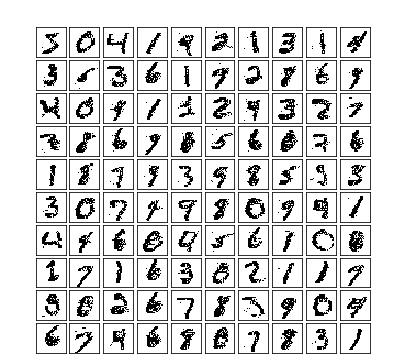
(d)

Figure 6: (a) is the original input image. (b) is the reconstructed image using  Gibbs sampling with  $w$  having $\mathbb{Z}_{3}$ as support. (c) is the reconstructed image with $w$ supported in $3^{3}\mathbb{Z}_{3}$. (d) is the reconstructed image with $w$ supported in $3^{4}\mathbb{Z}_{3}$.

7 Apendix A: Basic facts on $p$-adic analysis

In this section we review some basic results on $p$-adic analysis required in this article. For a detailed exposition on $p$-adic analysis the reader may consult [20], [43]-[45]. For a quick review of $p$-adic analysis the reader may consult [46].

7.1 The field of $p$-adic numbers

The field of $p-$adic numbers $\mathbb{Q}_{p}$ is defined as the completion of the field of rational numbers $\mathbb{Q}$ with respect to the $p-$adic norm $|\cdot|_{p}$, which is defined as

$$|x|_{p}=\begin{cases}0&\text{if }x=0\\ p^{-\gamma}&\text{if }x=p^{\gamma}\dfrac{a}{b},\end{cases}$$ (3)

where $a$ and $b$ are integers coprime with $p$. The integer $\gamma=ord_{p}(x):=ord(x)$, with $ord(0):=+\infty$, is called the $p-$adic order of $x$. The metric space $\left(\mathbb{Q}_{p},\left|\cdot\right|_{p}\right)$ is a complete ultrametric space. Ultrametric means that $\left|x+y\right|_{p}\leq\max\left\{\left|x\right|_{p},\left|y\right|_{p}\right\}$. As a topological space $\mathbb{Q}_{p}$ is homeomorphic to a Cantor-like subset of the real line, see, e.g., [20], [37], [43].

Any $p-$adic number $x\neq 0$ has a unique expansion of the form

$$x=p^{ord(x)}\sum_{j=0}^{\infty}x_{j}p^{j},$$

where $x_{j}\in\{0,1,2,\dots,p-1\}$ and $x_{0}\neq 0$. In addition, for any $x\in\mathbb{Q}_{p}\smallsetminus\left\{0\right\}$ we have

$$\left|x\right|_{p}=p^{-ord(x)}.$$

7.2 Topology of $\mathbb{Q}_{p}$

For $r\in\mathbb{Z}$, denote by $B_{r}(a)=\{x\in\mathbb{Q}_{p};\left|x-a\right|_{p}\leq p^{r}\}$ the ball of radius $p^{r}$ with center at $a\in\mathbb{Q}_{p}$, and take $B_{r}(0):=B_{r}$. The ball $B_{0}$ equals the ring of $p-$adic integers $\mathbb{Z}_{p}$. The balls are both open and closed subsets in $\mathbb{Q}_{p}$. We use $\Omega\left(p^{-r}\left|x-a\right|_{p}\right)$ to denote the characteristic function of the ball $B_{r}(a)$. Two balls in $\mathbb{Q}_{p}$ are either disjoint or one is contained in the other. As a topological space $\left(\mathbb{Q}_{p},\left|\cdot\right|_{p}\right)$ is totally disconnected, i.e., the only connected  subsets of $\mathbb{Q}_{p}$ are the empty set and the points. A subset of $\mathbb{Q}_{p}$ is compact if and only if it is closed and bounded in $\mathbb{Q}_{p}$, see e.g. [20, Section 1.3], or [43, Section 1.8]. The balls and spheres are compact subsets. Thus $\left(\mathbb{Q}_{p},\left|\cdot\right|_{p}\right)$ is a locally compact topological space.

7.2.1 Tree-like structures

Any $p$-adic integer $i$ admits an expansion of the form $i=i_{k}p^{k}+i_{k+1}p^{k+1}+\ldots$ for some $k\geq 0,i_{k}\neq 0$. The set of $p$-adic truncated integers modulo $p^{l}$, $l\geq 1$, consists of all the integers of the form $i\boldsymbol{=}i_{0}+i_{1}p+\ldots+i_{l-1}p^{l-1}$. These numbers form a complete set of representatives for the elements of the additive group $G_{l}=\mathbb{Z}_{p}/p^{l}\mathbb{Z}_{p}$, which is isomorphic to the set of integers $\mathbb{Z}/p^{l}\mathbb{Z}$ (written in base $p$) modulo $p^{l}$. By restricting $\left|\cdot\right|_{p}$ to $G_{l}$, it becomes a normed space, and $\left|G_{l}\right|_{p}=\left\{0,p^{-\left(l-1\right)},\cdots,p^{-1},1\right\}$. With the metric induced by $\left|\cdot\right|_{p}$, $G_{l}$ becomes a finite ultrametric space. In addition, $G_{l}$ can be identified with the set of branches (vertices at the top level) of a rooted tree with $l+1$ levels and $p^{l}$ branches. By definition the root of the tree is the only vertex at level $0$. There are exactly $p$ vertices at level $1$, which correspond with the possible values of the digit $i_{0}$ in the $p$-adic expansion of $i$. Each of these vertices is connected to the root by a non-directed edge. At level $k$, with $2\leq k\leq l+1$, there are exactly $p^{k}$ vertices,  each vertex corresponds to a truncated expansion of $i$ of the form $i_{0}+\cdots+i_{k-1}p^{k-1}$. The vertex corresponding to $i_{0}+\cdots+i_{k-1}p^{k-1}$ is connected to a vertex $i_{0}^{\prime}+\cdots+i_{k-2}^{\prime}p^{k-2}$ at the level $k-1$ if and only if $\left(i_{0}+\cdots+i_{k-1}p^{k-1}\right)-\left(i_{0}^{\prime}+\cdots+i_{k-2}^{\prime}p^{k-2}\right)$ is divisible by $p^{k-1}$. See Figure 1. The balls $B_{-r}(a)=a+p^{r}\mathbb{Z}_{p}$ are an infinite rooted trees.

7.3 The Haar measure

Since $(\mathbb{Z}_{p},+)$ is a locally compact topological group, there exists a Haar measure $dx$, which is invariant under translations, i.e., $d(x+a)=dx$, [47]. If we normalize this measure by the condition $\int_{\mathbb{Z}_{p}}dx=1$, then $dx$ is unique. It follows immediately that

$${\textstyle\int\limits_{B_{r}(a)}}dx={\textstyle\int\limits_{a+p^{-r}\mathbb{Z}_{p}}}dx=p^{r}{\textstyle\int\limits_{\mathbb{Z}_{p}}}dy=p^{r}\text{, }r\in\mathbb{Z}\text{.}$$

In a few ocassions we use the two-dimensional Haar measure $dxdy$ of the additive group $(\mathbb{Z}_{p}\times\mathbb{Z}_{p},+)$ normalize this measure by the condition $\int_{\mathbb{Z}_{p}}\int_{\mathbb{Z}_{p}}dxdy=1$. For a quick review of the integration in the $p$-adic framework the reader may consult [46] and the references therein.

7.4 The Bruhat-Schwartz space in the unit ball

A real-valued function $\varphi$ defined on $\mathbb{Z}_{p}$ is called Bruhat-Schwartz function (or a test function) if for any $x\in\mathbb{Z}_{p}$ there exist an integer $l(x)\in\mathbb{Z}$ such that

$$\varphi(x+x^{\prime})=\varphi(x)\text{ for any }x^{\prime}\in B_{l(x)}.$$ (4)

The $\mathbb{R}$-vector space of Bruhat-Schwartz functions supported in the unit ball is denoted by $\mathcal{D}(\mathbb{Z}_{p})$. For $\varphi\in\mathcal{D}(\mathbb{Z}_{p})$, the largest number $l=l(\varphi)$ satisfying (4) is called the exponent of local constancy (or the parameter of constancy) of $\varphi$. A function $\varphi$ in $\mathcal{D}(\mathbb{Z}_{p})$ can be written as

$$\varphi\left(x\right)={\displaystyle\sum\limits_{j=1}^{M}}\varphi\left(\widetilde{x}_{j}\right)\Omega\left(p^{r_{j}}\left|x-\widetilde{x}_{j}\right|_{p}\right),$$

where the $\widetilde{x}_{j}$, $j=1,\ldots,M$, are points in $\mathbb{Z}_{p}$, the $r_{j}$, $j=1,\ldots,M$, are integers, and $\Omega\left(p^{r_{j}}\left|x-\widetilde{x}_{j}\right|_{p}\right)$ denotes the characteristic function of the ball $B_{-r_{j}}(\widetilde{x}_{j})=\widetilde{x}_{j}+p^{r_{j}}\mathbb{Z}_{p}$.

8 Appendix B: Discretization of the energy functional

The elments of $G_{l}=\mathbb{Z}_{p}/p^{l}\mathbb{Z}_{p}$, $l\geq 1$, have the form $i\boldsymbol{=}i_{0}+i_{1}p+\ldots+i_{l-1}p^{l-1}$, where the $i_{k}$s are $p$-adic digits. We denote by $\mathcal{D}^{l}(\mathbb{Z}_{p})$ the $\mathbb{R}$-vector space of all test functions of the form

$$\varphi\left(x\right)={\textstyle\sum\limits_{i\in G_{l}}}\varphi\left(i\right)\Omega\left(p^{l}\left|x-i\right|_{p}\right)\text{, \ }\varphi\left(i\right)\in\mathbb{R}\text{,}$$

here $\Omega\left(p^{l}\left|x-i\right|_{p}\right)$ is the characteristic function of the ball $i+p^{l}\mathbb{Z}_{p}$. Notice that $\varphi$ is supported on $\mathbb{Z}_{p}$ and that $\mathcal{D}^{l}(\mathbb{Z}_{p})$ is a finite dimensional vector space spanned by the basis $\left\{\Omega\left(p^{l}\left|x-i\right|_{p}\right)\right\}_{i\in G_{l}}$.

By identifying $\varphi\in\mathcal{D}^{l}(\mathbb{Z}_{p})$ with the column vector $\left[\varphi\left(i\right)\right]_{i\in G_{l}}\in\mathbb{R}^{\#G_{l}}$, we get that $\mathcal{D}^{l}(\mathbb{Z}_{p})$ is isomorphic to $\mathbb{R}^{\#G_{l}}$ endowed with the norm $\left\|\left[\varphi\left(i\right)\right]_{i\in G_{l}^{N}}\right\|=\max_{i\in G_{l}}\left|\varphi\left(i\right)\right|$. Furthermore,

$$\mathcal{D}^{l}\hookrightarrow\mathcal{D}^{l+1}\hookrightarrow\mathcal{D}(\mathbb{Z}_{p}),$$

where $\hookrightarrow$ denotes a continuous embedding.

The restriction of $E$ to the subspace $\mathcal{D}^{l}(\mathbb{Z}_{p})$ gives a discretization of $E$ denoted as $E_{l}$. Indeed, by assuming that

$$\boldsymbol{v}\left(x\right) ={\textstyle\sum\limits_{i\in G_{l}}}\boldsymbol{v}\left(i\right)\Omega\left(p^{l}\left|x-i\right|_{p}\right)\text{,}$$

$$\boldsymbol{h}\left(x\right) ={\textstyle\sum\limits_{i\in G_{l}}}\boldsymbol{h}\left(i\right)\Omega\left(p^{l}\left|x-i\right|_{p}\right),$$

we have

$${\displaystyle\iint\limits_{\mathbb{Z}_{p}\times\mathbb{Z}_{p}}}w\left(x-y\right)\Omega\left(p^{l}\left|x-i\right|_{p}\right)\Omega\left(p^{l}\left|y-j\right|_{p}\right)dxdy$$

$$=\iint\limits_{p^{l}\mathbb{Z}_{p}\times p^{l}\mathbb{Z}_{p}}w((i-j)+(x-y))dxdy,$$

and by using that $a\left(x\right)$, $b(x)$, $c(x)$, $d(x)$ are test functions supported in the unit ball, and taking $l$ sufficiently large, we have

$$a\left(x\right)\Omega\left(p^{l}\left|x-i\right|_{p}\right)=a\left(i\right)\Omega\left(p^{l}\left|x-i\right|_{p}\right)\text{, }$$

$$b(x)\Omega\left(p^{l}\left|x-i\right|_{p}\right)=b(i)\Omega\left(p^{l}\left|x-i\right|_{p}\right),$$

$$c\left(x\right)\Omega\left(p^{l}\left|x-i\right|_{p}\right)=c\left(i\right)\Omega\left(p^{l}\left|x-i\right|_{p}\right)\text{,}$$

$$\text{ }d(x)\Omega\left(p^{l}\left|x-i\right|_{p}\right)=d(i)\Omega\left(p^{l}\left|x-i\right|_{p}\right),$$

and consequently

$$E_{l}\left(\boldsymbol{v},\boldsymbol{h}\right)=-{\displaystyle\sum\limits_{\begin{subarray}{c}i,\text{ }j\in G_{l}\\ i\neq j\end{subarray}}}\boldsymbol{v}\left(i\right)\boldsymbol{h}\left(j\right)\left(\text{ }\iint\limits_{p^{l}\mathbb{Z}_{p}\times p^{l}\mathbb{Z}_{p}}w(i-j+x-y)dxdy\right)$$

$$-p^{-l}{\displaystyle\sum\limits_{i\in G_{l}}}a\left(i\right)\boldsymbol{v}\left(i\right)-p^{-l}{\displaystyle\sum\limits_{i\in G_{l}}}b\left(i\right)\boldsymbol{h}\left(i\right)+\frac{ep^{-l}}{2}{\displaystyle\sum\limits_{\boldsymbol{i}\in G_{l}}}\boldsymbol{v}^{2}\left(i\right)+\frac{ep^{-l}}{2}{\displaystyle\sum\limits_{\boldsymbol{i}\in G_{l}}}\boldsymbol{h}^{2}\left(i\right)$$

$$+\frac{p^{-l}}{2}{\displaystyle\sum\limits_{i\in G_{l}}}c\left(i\right)\boldsymbol{v}^{4}\left(i\right)+\frac{p^{-l}}{2}{\displaystyle\sum\limits_{i\in G_{l}}}d\left(i\right)\boldsymbol{h}^{4}\left(i\right).$$

We take $v_{i}=\boldsymbol{v}\left(i\right)$, $h_{i}=\boldsymbol{h}\left(i\right)$,

$$w_{i-j}=\iint\limits_{p^{l}\mathbb{Z}_{p}\times p^{l}\mathbb{Z}_{p}}w((i-j)+(x-y))dxdy,$$

$a_{i}=p^{-l}a\left(i\right)$, $b_{i}=p^{-l}b\left(i\right)$, $c_{i}=p^{-l}c\left(i\right)$, $d_{i}=p^{-l}d\left(i\right)$, for $i$, $j\in G_{l}$, and $\boldsymbol{\theta}=\left\{w_{ij},a_{i},b_{i},c_{i},d_{i}\right\}$. We also rescale $e$ to $ep^{l}$, then

$$E_{l}\left(\boldsymbol{v},\boldsymbol{h};\boldsymbol{\theta}\right)=-{\sum\limits_{i,\text{ }j\in G_{l}}}w_{i-j}v_{i}h_{j}-{\displaystyle\sum\limits_{i\in G_{l}}}a_{i}v_{i}-{\displaystyle\sum\limits_{i\in G_{l}}}b_{i}h_{i}$$

$$+\frac{e}{2}{\displaystyle\sum\limits_{i\in G_{l}}}v_{i}^{2}+\frac{e}{2}{\displaystyle\sum\limits_{i\in G_{l}}}h_{i}^{2}+{\displaystyle\sum\limits_{i\in G_{l}}}c_{i}v_{i}^{4}+{\displaystyle\sum\limits_{i\in G_{l}}}d_{i}h_{i}^{4}\text{.}$$

We now recall that $G_{l}$ is an additive group, then

$${\displaystyle\sum\limits_{i,\text{ }j\in G_{l}}}w_{i-j}v_{i}h_{j}={\displaystyle\sum\limits_{j\in G_{l}}}{\displaystyle\sum\limits_{k\in G_{l}}}w_{k}v_{j+k}h_{j},$$

and consequently

$$E_{l}\left(\boldsymbol{v},\boldsymbol{h};\boldsymbol{\theta}\right)=-{\displaystyle\sum\limits_{j\in G_{l}}}{\displaystyle\sum\limits_{k\in G_{l}}}w_{k}v_{j+k}h_{j}-{\displaystyle\sum\limits_{j\in G_{l}}}a_{j}v_{j}-{\displaystyle\sum\limits_{j\in G_{l}}}b_{j}h_{j}$$

$$+\frac{e}{2}{\displaystyle\sum\limits_{j\in G_{l}^{N}}}v_{j}^{2}+\frac{e}{2}{\displaystyle\sum\limits_{j\in G_{l}}}h_{j}^{2}+{\displaystyle\sum\limits_{j\in G_{l}}}c_{j}v_{j}^{4}+{\displaystyle\sum\limits_{j\in G_{l}}}d_{j}h_{j}^{4}\text{.}$$

9 Appendix C: Some probability distributions

From now on, we assume that visible and hidden fields are binary variables. However, most of our mathematical formulation is valid under the assumption that visible and hidden fields are discrete variables. We set

$$\boldsymbol{V}=\{V_{1},V_{2},\ldots,V_{N}\},\quad\boldsymbol{H}=\{H_{1},H_{2},\ldots,H_{N}\},$$

$N=p^{l}$, to be the respective visible and hidden random variable sets. The random variables $(\boldsymbol{V},\boldsymbol{H})$ take values $(\boldsymbol{v},\boldsymbol{h})\in\{0,1\}^{2N}$. For the sake of simplicity, we will identify the random vector $\boldsymbol{V}$ with $\boldsymbol{v}$, and the random vector $\boldsymbol{H}$ with $\boldsymbol{h}$. We identify $G_{l}$ with the set of branches (vertices at the top level) of a rooted tree with $l+1$ levels and $p^{l}$ branches. Attached to each branch $i\in G_{l}$ there are two are two states: $v_{i}$, $h_{i}$. With this notation, $\boldsymbol{v}=\left[v_{i}\right]_{i\in G_{l}}$ is a realization of the visible field, and $\boldsymbol{h}=\left[h_{i}\right]_{i\in G_{l}}$ is a realization of the hidden field. The joint distribution of the random vectors $(\boldsymbol{v},\boldsymbol{h})$ is given by the following Boltzmann probability distribution:

$$\boldsymbol{P}_{l}(\boldsymbol{v},\boldsymbol{h};\boldsymbol{\theta})=\frac{\exp\left(-E_{l}\left((\boldsymbol{v},\boldsymbol{h};\boldsymbol{\theta})\right)\right)}{Z_{l}},$$ (5)

where

$$Z_{l}={\sum\limits_{\boldsymbol{v},\boldsymbol{h}}}\exp\left(-E_{l}\left(\boldsymbol{v},\boldsymbol{h};\boldsymbol{\theta}\right)\right),$$

and $E_{l}$ is defined in Equation 1

By using the joint distribution of the visible field and the hidden field (5), we compute the marginal probability distributions as follows:

$$\boldsymbol{P}_{l}(\boldsymbol{v};\boldsymbol{\theta})={\displaystyle\sum\limits_{\boldsymbol{h}}}\boldsymbol{P}_{l}(\boldsymbol{v},\boldsymbol{h};\boldsymbol{\theta})=\frac{{\sum\limits_{\boldsymbol{h}}}\exp\left(-E_{l}\left(\boldsymbol{v},\boldsymbol{h};\boldsymbol{\theta}\right)\right)}{{\displaystyle\sum\limits_{\boldsymbol{v},\boldsymbol{h}}}\exp\left(-E_{l}\left(\boldsymbol{v},\boldsymbol{h};\boldsymbol{\theta}\right)\right)},$$

$$\boldsymbol{P}_{l}(\boldsymbol{h};\boldsymbol{\theta})={\displaystyle\sum\limits_{\boldsymbol{v}}}\boldsymbol{P}_{l}(\boldsymbol{v},\boldsymbol{h};\boldsymbol{\theta})=\frac{{\displaystyle\sum\limits_{\boldsymbol{v}}}\exp\left(-E_{l}\left(\boldsymbol{v},\boldsymbol{h};\boldsymbol{\theta}\right)\right)}{{\displaystyle\sum\limits_{\boldsymbol{v},\boldsymbol{h}}}\exp\left(-E_{l}\left(\boldsymbol{v},\boldsymbol{h};\boldsymbol{\theta}\right)\right)}.$$

Since we are assuming that $\boldsymbol{v},\boldsymbol{h}$ are binary, the energy functional takes the form

$$E_{l}(\boldsymbol{v},\boldsymbol{h};\boldsymbol{\theta})=-\sum_{k\in G_{l}}\sum_{j\in G_{l}}w_{k}v_{j+k}h_{j}-\sum_{j\in G_{l}}a_{j}v_{j}-\sum_{j\in G_{l}}b_{j}h_{j}.$$

The classical RBM has the advantage of independence between the visible units as well as the hidden units. The $p$-adic BM shares the same advantage, i.e., by fixing the hidden field $\boldsymbol{h}$, the random variables $v_{i}$, $i\in G_{l}$, become independent. An analog assertion is valid if we fix the visible field $\boldsymbol{v}$. More precisely, the conditional probability distributions satisfy

$$\boldsymbol{P}_{l}(\boldsymbol{v}\mid\boldsymbol{h};\boldsymbol{\theta})={\prod\limits_{j\in G_{l}}}\boldsymbol{P}_{l}\left(v_{j}\mid\boldsymbol{h};\boldsymbol{\theta}\right),\quad\mbox{and}\quad\boldsymbol{P}_{l}(\boldsymbol{h}\mid\boldsymbol{v};\boldsymbol{\theta})={\displaystyle\prod\limits_{j\in G_{l}}}\boldsymbol{P}_{l}\left(h_{j}\mid\boldsymbol{v};\boldsymbol{\theta}\right).$$

Indeed, by direct computation, we have

$$\boldsymbol{P}_{l}(\boldsymbol{v}\mid\boldsymbol{h};\boldsymbol{\theta})=\frac{\boldsymbol{P}_{l}(\boldsymbol{v},\boldsymbol{h};\boldsymbol{\theta})}{\boldsymbol{P}_{l}(\boldsymbol{h};\boldsymbol{\theta})}$$

$$= \frac{\exp\left(-E_{l}\left(\boldsymbol{v},\boldsymbol{h};\boldsymbol{\theta}\right)\right)}{{\displaystyle\sum\limits_{\boldsymbol{v}}}\exp\left(-E_{l}\left(\boldsymbol{v},\boldsymbol{h};\boldsymbol{\theta}\right)\right)}=\frac{{\displaystyle\prod\limits_{j\in G_{l}}}\exp\left({\displaystyle\sum\limits_{k\in G_{l}}}w_{k}v_{j}h_{j-k}+a_{j}v_{j}\right)}{{\displaystyle\sum\limits_{\boldsymbol{v}}}{\displaystyle\prod\limits_{j\in G_{l}}}\exp\left({\displaystyle\sum\limits_{k\in G_{l}}}w_{k}v_{j}h_{j-k}+a_{j}v_{j}\right)}$$

$$= {\displaystyle\prod\limits_{j\in G_{l}}}\frac{\exp\left(v_{j}{\displaystyle\sum\limits_{k\in G_{l}}}w_{k}h_{j-k}+a_{j}v_{j}\right)}{{\displaystyle\sum\limits_{v_{j}}}\exp\left(v_{j}{\displaystyle\sum\limits_{k\in G_{l}}}w_{k}h_{j-k}+a_{j}v_{j}\right)}={\displaystyle\prod\limits_{j\in G_{l}}}\frac{\boldsymbol{P}_{l}\left(v_{j},\boldsymbol{h};\boldsymbol{\theta}\right)}{{\displaystyle\sum\limits_{v_{j}}}\boldsymbol{P}_{l}\left(v_{j},\boldsymbol{h};\boldsymbol{\theta}\right)}={\displaystyle\prod\limits_{j\in G_{l}}}\boldsymbol{P}_{l}\left(v_{j}\mid\boldsymbol{h};\boldsymbol{\theta}\right).$$

Similarly, we can prove that

$$\boldsymbol{P}_{l}(\boldsymbol{h}\mid\boldsymbol{v};\boldsymbol{\theta})={\prod\limits_{j\in G_{l}}}\boldsymbol{P}_{l}\left(h_{j}\mid\boldsymbol{v};\boldsymbol{\theta}\right).$$ (6)

9.1 Gradient of the Log-likelihood

The log-likelihood giving a single visible state $\boldsymbol{v}$ is given

$$\ln\boldsymbol{P}_{l}(\boldsymbol{v}|\boldsymbol{\theta})=\ln\dfrac{1}{Z}\sum_{\boldsymbol{h}}e^{-E(\boldsymbol{v},\boldsymbol{h})}=\ln\sum_{\boldsymbol{h}}e^{-E(\boldsymbol{v},\boldsymbol{h})}-\ln\sum_{\boldsymbol{h},\boldsymbol{v}}e^{-E(\boldsymbol{v},\boldsymbol{h})}.$$

Taking the derivative with respect to the parameters gives the following mean-like representation:

$$\begin{split}&\dfrac{\partial}{\partial\boldsymbol{\theta}}\ln\boldsymbol{P}_{l}(\boldsymbol{v}|\boldsymbol{\theta})=\dfrac{\partial}{\partial\boldsymbol{\theta}}\ln\sum_{\boldsymbol{h}}e^{-E(\boldsymbol{v},\boldsymbol{h})}-\dfrac{\partial}{\partial\boldsymbol{\theta}}\ln\sum_{\boldsymbol{h},\boldsymbol{v}}e^{-E(\boldsymbol{v},\boldsymbol{h})}\\ =&-\dfrac{1}{\sum\limits_{\boldsymbol{h}}e^{-E(\boldsymbol{v},\boldsymbol{h})}}\sum_{\boldsymbol{h}}e^{-E(\boldsymbol{v},\boldsymbol{h})}\dfrac{\partial}{\partial\boldsymbol{\theta}}E(\boldsymbol{v},\boldsymbol{h})+\dfrac{1}{\sum\limits_{\boldsymbol{v},\boldsymbol{h}}e^{-E(\boldsymbol{v},\boldsymbol{h})}}\sum_{\boldsymbol{v},\boldsymbol{h}}e^{-E(\boldsymbol{v},\boldsymbol{h})}\dfrac{\partial}{\partial\boldsymbol{\theta}}E(\boldsymbol{v},\boldsymbol{h})\\ =&-\sum_{\boldsymbol{h}}\boldsymbol{P}_{l}(\boldsymbol{h}|\boldsymbol{v})\dfrac{\partial}{\partial\boldsymbol{\theta}}E(\boldsymbol{v},\boldsymbol{h})+\sum_{\boldsymbol{v},\boldsymbol{h}}\boldsymbol{P}_{l}(\boldsymbol{v},\boldsymbol{h})\dfrac{\partial}{\partial\boldsymbol{\theta}}E(\boldsymbol{v},\boldsymbol{h}).\end{split}$$ (7)

In the case of multiple visible states $S=\{\boldsymbol{v}_{1},\boldsymbol{v}_{2},\cdots,\boldsymbol{v}_{s}\}$, the log-likelihood is defined in the average sense, i.e., $\dfrac{1}{s}\sum\limits_{\boldsymbol{v}\in S}\ln\boldsymbol{P}_{l}(\boldsymbol{v}|\boldsymbol{\theta})$.

Taking the derivative with respect to $w_{k}$ gives

$$\begin{split}&\dfrac{\partial}{\partial w_{k}}\ln\boldsymbol{P}_{l}(\boldsymbol{v}|\boldsymbol{\theta})=\sum_{\boldsymbol{h}}\left(\boldsymbol{P}_{l}(\boldsymbol{h}|\boldsymbol{v})\sum_{j\in G_{l}}v_{j+k}h_{j}\right)-\sum_{\boldsymbol{v},\boldsymbol{h}}\left(\boldsymbol{P}_{l}(\boldsymbol{h},\boldsymbol{v})\sum_{j\in G_{l}}v_{j+k}h_{j}\right)\\ =&\sum_{\boldsymbol{h}}\left(\boldsymbol{P}_{l}(\boldsymbol{h}|\boldsymbol{v})\sum_{j\in G_{l}}v_{j+k}h_{j}\right)-\sum_{\boldsymbol{v}}\boldsymbol{P}_{l}(\boldsymbol{v})\left(\sum_{\boldsymbol{h}}\left(\boldsymbol{P}_{l}(\boldsymbol{h}|\boldsymbol{v})\sum_{j\in G_{l}}v_{j+k}h_{j}\right)\right).\end{split}$$ (8)

Now, let $\mathbb{I}$ be the ordered indexes of all the positive states in $\boldsymbol{v}$.

$$\begin{split}&\sum_{\boldsymbol{h}}\left(\boldsymbol{P}_{l}(\boldsymbol{h}|\boldsymbol{v})\sum_{i\in G_{l}}v_{i+k}h_{i}\right)=\sum_{\boldsymbol{h}}\boldsymbol{P}_{l}(\boldsymbol{h}|\boldsymbol{v})\left(\sum_{i\in\mathbb{I}}h_{i-k}\right)\\ =&\sum_{\boldsymbol{h}_{{\mathbb{I}}}}\sum_{\boldsymbol{h}_{G_{l}\setminus\mathbb{I}}}\prod_{i\in\ \mathbb{I}}\boldsymbol{P}_{l}(h_{i-k}|\boldsymbol{v})\prod_{i\in G_{l}\setminus\ \mathbb{I}}\boldsymbol{P}_{l}(h_{i-k}|\boldsymbol{v})\left(\sum_{i\in\ \mathbb{I}}h_{i-k}\right)\\ =&\left(\sum_{\boldsymbol{h}_{{\mathbb{I}}}}\prod_{i\in\ \mathbb{I}}\boldsymbol{P}_{l}(h_{i-k}|\boldsymbol{v})\left(\sum_{i\in\ \mathbb{I}}h_{i-k}\right)\right)\underbrace{\left(\sum_{\boldsymbol{h}_{G_{l}\setminus\ \mathbb{I}}}\prod_{i\in G_{l}\setminus\ \mathbb{I}}\boldsymbol{P}_{l}(h_{i-k}|\boldsymbol{v})\right)}_{=1}\\ =&\sum_{\boldsymbol{h}_{{\mathbb{I}}}}\left(\displaystyle\prod_{i\in{{\mathbb{I}}}}\boldsymbol{P}_{l}(h_{i-k}|\boldsymbol{v})\sum_{i\in{{\mathbb{I}}}}h_{i-k}\right)\\ =&\sum_{{i\in\ \mathbb{I}}}\boldsymbol{P}_{l}(h_{i-k}=1|\boldsymbol{v})=\sum_{i\in G_{l}}\boldsymbol{P}_{l}(h_{i-k}=1|\boldsymbol{v})v_{i}.\end{split}$$ (9)

Combing eq. 8 and eq. 9 gives

$$\frac{\partial\log\boldsymbol{P}_{l}(\boldsymbol{v}|\boldsymbol{\theta})}{w_{k}}=\sum_{i\in G_{l}}\boldsymbol{P}_{l}(h_{i-k}=1|\boldsymbol{v})v_{i}-\sum_{\boldsymbol{v}}\boldsymbol{P}_{l}(\boldsymbol{v})\left(\sum_{i\in G_{l}}\boldsymbol{P}_{l}(h_{i-k}=1|\boldsymbol{v})v_{i}\right).$$ (10)

Note that the above formula is different from the classical RBM, [48, Formula 29].

We derive the derivatives with respect to $a_{j}$ and $b_{j}$ similarly as in the classical RBM:

$$\dfrac{\partial}{\partial a_{j}}\ln\boldsymbol{P}_{l}(\boldsymbol{v}|\boldsymbol{\theta})=-\sum_{\boldsymbol{h}}\boldsymbol{P}_{l}(\boldsymbol{h}|\boldsymbol{v})\dfrac{\partial}{\partial a_{j}}E_{l}(\boldsymbol{v},\boldsymbol{h})+\sum_{\boldsymbol{v},\boldsymbol{h}}\boldsymbol{P}_{l}(\boldsymbol{h},\boldsymbol{v})\dfrac{\partial}{\partial a_{j}}E_{l}(\boldsymbol{v},\boldsymbol{h})$$

$$=\sum_{\boldsymbol{h}}\boldsymbol{P}_{l}(\boldsymbol{h}|\boldsymbol{v})v_{j}-\sum_{\boldsymbol{v},\boldsymbol{h}}\boldsymbol{P}_{l}(\boldsymbol{h},\boldsymbol{v})v_{j}=v_{j}-\sum_{\boldsymbol{v}}\boldsymbol{P}_{l}(\boldsymbol{v})v_{j},$$ (11)

and

$$\dfrac{\partial}{\partial b_{j}}\ln\boldsymbol{P}_{l}(\boldsymbol{v}|\boldsymbol{\theta})=-\sum_{\boldsymbol{h}}\boldsymbol{P}_{l}(\boldsymbol{h}|\boldsymbol{v})\dfrac{\partial}{\partial b_{j}}E_{l}(\boldsymbol{v},\boldsymbol{h})+\sum_{\boldsymbol{v},\boldsymbol{h}}\boldsymbol{P}_{l}(\boldsymbol{h},\boldsymbol{v})\dfrac{\partial}{\partial b_{j}}E_{l}(\boldsymbol{v},\boldsymbol{h})$$

$$=\sum_{\boldsymbol{h}}\boldsymbol{P}_{l}(\boldsymbol{h}|\boldsymbol{v})h_{j}-\sum_{\boldsymbol{v},\boldsymbol{h}}\boldsymbol{P}_{l}(\boldsymbol{h},\boldsymbol{v})h_{j}=\boldsymbol{P}_{l}(h_{j}=1|\boldsymbol{v})-\sum_{\boldsymbol{v}}\boldsymbol{P}_{l}(h_{j}=1|\boldsymbol{v}).$$ (12)

9.2 Contrastive divergence learning

As in the classical case, the exact computation of the gradient of the log-likelihood involves an exponential number of terms, see (10). We adopt the contrastive divergence (CD) method, introduced by Hinton [49], to the $p$-adic case to approximate the minimization of the gradient of the log-likelihood.

The approximation of eq. 10 –eq. 13 using the contrastive convergence method can be represented as follows:

$$\begin{split}&\frac{\partial\log\boldsymbol{P}_{l}(\boldsymbol{v}|\boldsymbol{\theta})}{w_{k}}\approx\sum_{{i\in G_{l}}}\boldsymbol{P}_{l}(h_{i-k}=1|\boldsymbol{v}^{(0)})v_{i}-\sum_{{i\in G_{l}}}\boldsymbol{P}_{l}(h_{i-k}=1|\boldsymbol{v}^{(m)})v_{i}^{(m)},\\ &\frac{\partial\log\boldsymbol{P}_{l}(\boldsymbol{v}|\boldsymbol{\theta})}{a_{j}}\approx v_{j}^{(0)}-v_{j}^{(m)},\\ &\frac{\partial\log\boldsymbol{P}_{l}(\boldsymbol{v}|\boldsymbol{\theta})}{b_{j}}\approx\boldsymbol{P}_{l}(h_{j}=1|\boldsymbol{v}^{(0)})-\boldsymbol{P}_{l}(h_{j}=1|\boldsymbol{v}^{(m)}),\end{split}$$ (13)

where $m$ is a pre-determined positive integer, $\boldsymbol{v}^{(0)}$ is a training example and $\boldsymbol{v}^{(m)}$ is a sample of the Gibbs chain after $m$ steps. More precisely, we implement the Gibbs sampling in the following way. First, we obtain a sample of $\boldsymbol{h}^{(0)}$ using the conditional distribution $P_{l}(\boldsymbol{h}|\boldsymbol{v^{(0)}})$. Then, we obtain a sample of $\boldsymbol{v}^{(1)}$ using $P_{l}(\boldsymbol{v}|\boldsymbol{h}^{(0)})$. We repeat this process until we get $\boldsymbol{v}^{(m)}$.

The following formulas are utilized in the calculation. Let $\boldsymbol{h}_{-i}$ denotes the state of all hidden units expect for the $i$-th one:

$$\boldsymbol{P}_{l}(h_{i}=1|\boldsymbol{v})=\boldsymbol{P}_{l}(h_{i}=1|\boldsymbol{h}_{-i},\boldsymbol{v})=\dfrac{\boldsymbol{P}_{l}(h_{i}=1,\boldsymbol{h}_{-i},\boldsymbol{v})}{\boldsymbol{P}_{l}(\boldsymbol{h}_{-i},\boldsymbol{v})}$$

$$=\dfrac{\boldsymbol{P}_{l}(h_{i}=1,\boldsymbol{h}_{-i},\boldsymbol{v})}{\boldsymbol{P}_{l}(h_{i}=1,\boldsymbol{h}_{-i},\boldsymbol{v})+\boldsymbol{P}_{l}(h_{i}=0,\boldsymbol{h}_{-i},\boldsymbol{v})}=\dfrac{1}{1+\dfrac{\boldsymbol{P}_{l}(h_{i}=0,\boldsymbol{h}_{-i},\boldsymbol{v})}{\boldsymbol{P}_{l}(h_{i}=1,\boldsymbol{h}_{-i},\boldsymbol{v})}}$$

$$=\dfrac{1}{1+\dfrac{1}{\exp\left(\sum\limits_{k\in G_{l}}w_{k}v_{i+k}+b_{i}\right)}}=:\sigma\left({\sum_{k\in G_{l}}w_{k}v_{i+k}+b_{i})}\right).$$

Similarly, we have

$$\begin{split}&\boldsymbol{P}_{l}(h_{i}=0|\boldsymbol{v})=\sigma\left(-{\sum_{k\in G_{l}}w_{k}v_{i+k}-b_{i}}\right),\\ &\boldsymbol{P}_{l}(v_{i}=1|\boldsymbol{h})=\sigma\left(\sum_{k\in G_{l}}w_{i-k}h_{k}+a_{i}\right),\\ &\boldsymbol{P}_{l}(v_{i}=0|\boldsymbol{h})=\sigma\left(-\sum_{k\in G_{l}}w_{i-k}h_{k}-a_{i}\right).\end{split}$$ (14)

References

[1]LeCun, Y., Bengio, Y. & Hinton, G. E. Deep learning.
Nature521, 436–444 (2015).
[2]Bahri Y., Kadmon J., Pennington J., Schoenholz S.S.,
Sohl-Dickstein J., Ganguli S. Statistical Mechanics of Deep Learning.Annual Review of Condensed Matter Physics11, 501-528 (2020).
[3]Buice Michael A., Chow Carson C. Beyond mean field
theory: statistical field theory for neural networks. J. Stat. Mech.
Theory Exp.3, P03003, 21 pp. (2013).
[4]Buice Michael A., Cowan Jack D., Field-theoretic approach to
fluctuation effects in neural networks. Phys. Rev. E75, no.
5, 051919, 14 pp. (2007).
[5]Bachtis D., Aarts G., & Lucini B. Quantum
field-theoretic machine learning. Physical Review D, 103
(7), 074510 pp. 14 (2021).
[6]Dyer E., Gur-Ari G. Asymptotics of wide networks from
Feynman diagrams. https://doi.org/10.48550/arXiv.1909.11304.
[7]Erbin H., Lahoche V., Ousmane Samary D. Nonperturbative
renormalization for the neural network-QFT correspondence. Mach. Learn.: Sci.
Technol. 3 015027 (2022).
[8]Halverson J., Maiti A. and Stoner K. Neural networks and quantum field theory. Mach. Learn. Sci. Technol.2, 035002 (2021).
[9]Maiti A., Stoner K. and Halverson J. Symmetry-via-duality:
Invariant neural network densities from parameter-space correlators. https://arxiv.org/abs/2106.00694.
[10]Helias Moritz, Dahmen David, Statistical field
theory for neural networks. Lecture Notes in Physics, 970 ( Springer, Cham, 2020).
[11]Yaida, S. (2020, August). Non-Gaussian processes and neural networks at finite widths. In Mathematical and Scientific Machine Learning (pp. 165-192). PMLR.
[12]Zúñiga-Galindo, W. A. (2023). p-adic statistical field theory and deep belief networks. Physica A: Statistical Mechanics and its Applications, 128492.
[13]Le Roux Nicolas, Bengio Yoshua. Representational
power of restricted Boltzmann machines and deep belief networks. Neural
Comput. 20 , no. 6, 1631–1649 (2008).
[18] Zambrano-Luna, B. A., Zúñiga-Galindo, W. A. (2023). p-adic cellular neural networks: Applications to image processing. Physica D: Nonlinear Phenomena, 133668.
[19]Volovich I. V., Number theory as the ultimate physical
theory. -Adic Numbers Ultrametric Anal. Appl. 2, 77–87 (2010).
[20]Vladimirov V. S., Volovich I. V., Zelenov E. I. -Adic analysis and mathematical physics (Singapore, World Scientific, 1994).
[21]Dragovich B., Khrennikov A. Yu., Kozyrev S. V., Volovich I.
V. On adic mathematical physics. Adic Numbers
Ultrametric Anal. Appl.1 (1), 1, 1–17 (2009).
[22]Lerner E. Y., Misarov M. D. Scalar models in adic quantum
field theory and hierarchical models. Theor. Math. Phys. 78,
248–257 (1989).
[23]Missarov M. D. Adic theory as a functional
equation problem. Lett. Math. Phys.39(3), 253-260
(1997).
[24]Missarov M. D. Adic renormalization group solutions and the
Euclidean renormalization group conjectures. p-Adic Numbers
Ultrametric Anal. Appl.4(2), 109-114 (2012)
[25]Khrennikov A. Yu. -Adic Valued
Distributions in Mathematical Physics (Dordrecht, Kluwer Academic Publishers, 1994).
[26]Kochubei Anatoly N., Sait-Ametov Mustafa R.
Interaction measures on the space of distributions over the field of -adic
numbers. Infin. Dimens. Anal. Quantum Probab. Relat. Top.6(3), 389–411 (2003).
[27]Khrennikov, Andrei, Kozyrev, Sergei, Zúñiga-Galindo, W. A. Ultrametric Equations and its Applications.
Encyclopedia of Mathematics and its Applications 168 (Cambridge, Cambridge
University Press, 2018).
[28]Zúñiga-Galindo W. A. Non-Archimedean white
noise, pseudodifferential stochastic equations, and massive Euclidean fields.
J. Fourier Anal. Appl.23 (2), 288–323 (2017)
[29]Mendoza-Martínez M. L., Vallejo J. A.,
Zúñiga-Galindo, W. A. Acausal quantum theory for non-Archimedean
scalar fields. Rev. Math. Phys. 31(4), 1950011, 46 pp. (2019).
[30]Arroyo-Ortiz, Edilberto, Zúñiga-Galindo, W. A.
Construction of -adic covariant quantum fields in the framework of white
noise analysis. Rep. Math. Phys.84(1), 1–34 (2019).
[31]Zúñiga-Galindo W. A., Non-Archimedean
statistical field theory, Rev. Math. Phys.34 (8), Paper No.
2250022, 41 pp. (2022).
[32]Liu Ding et al. Machine learning by unitary tensor
network of hierarchical tree structure. New J. Phys.21,
073059 (2019).
[33]Cheng Song, Wang Lei, Xiang Tao, and Zhang Pan. Tree
tensor networks for generative modeling. Phys. Rev. B 99, 155131 (2019).
[34]Li Sujie, Feng Pan, Zhou Pengfei, and Zhang Pan.
Boltzmann machines as two-dimensional tensor networks. Phys. Rev. B
104, 075154 (2021).
[35]Orús, R. Tensor networks for complex quantum systems. Nat
Rev Phys 1, 538–550 (2019).
[36]KoblitzNeal. -Adic Numbers, -adic Analysis, and Zeta-Functions. Graduate Texts in Mathematics
No. 58 (New York, Springer-Verlag, 1984).
[37]Chistyakov D. V. Fractal geometry of images of continuous
embeddings of p-adic numbers and solenoids into Euclidean
spaces.Theoret. and Math. Phys.109 (1996), no. 3,
1495–1507 (1997).
[38]Honglak Lee, Roger Grosse, Rajesh Ranganath, and
Andrew Y. Ng. Unsupervised Learning of Hierarchical Representations with
Convolutional Deep Belief Networks. Communications of the ACM, vol.
54, no. 10, pp. 95-103 (2011).
[39]Le Roux Nicolas, Bengio Yoshua. Deep belief networks
are compact universal approximators. Neural Comput.22, no.
8, 2192–2207 (2010).
[40]Kleinert Hagen, Schulte-Frohlinde V. Critical
properties of -theories (Singapore, World Scientific, 2001).
[41]Mussardo Giuseppe. Statistical Field Theory. An
Introduction to Exactly Solved Models of Statistical Physics (Oxford , Oxford
University Press, 2010).
[42]G. E. Hinton, R.R. Salakhutdinov. Reducing the
dimensionality of data with neural networks. Science313,
5786 (2006), doi: 10.1126/science.112764.
[43]Albeverio S., Khrennikov A. Yu., Shelkovich V. M.
Theory of -adicdistributions: linear and nonlinear models
(Cambridge University Press, Cambridge 2010).
[44]Kochubei Anatoly N. Pseudo-differential equations and
stochastics over non-Archimedean fields (New York, Marcel Dekker, 2001).
[45]Taibleson M. H. Fourier analysis on local fields
(Princeton University Press, 1975).
[46]Bocardo-Gaspar Miriam, García-Compeán H.,
Zúñiga-Galindo W. A. Regularization of p-adic string amplitudes, and
multivariate local zeta functions. Lett. Math. Phys.109,
no. 5, 1167–1204 (2019).
[47]Halmos P. Measure Theory (D. Van Nostrand Company
Inc., New York, 1950).
[48]Fischer A., Igel C. An Introduction to
Restricted Boltzmann Machines. In: Alvarez, L., Mejail, M., Gomez, L.,
Jacobo, J. (eds) Progress in Pattern Recognition, Image Analysis, Computer
Vision, and Applications. CIARP 2012. Lecture Notes in Computer Science, vol
7441. Springer, Berlin, Heidelberg. https://doi.org/10.1007/978-3-642-33275-3_2.
[49]Hinton G. E., Training products of experts by minimizing
contrastive divergence, Neural Comput. 14, no. 8, pp.
1771–1800 (2002).
[50]D. Koller and N. Friedman, Probabilistic Graphical
Models: Principles and Techniques (The MIT Press, Cambridge, MA, 2009).