pyTDGL: Time-dependent Ginzburg-Landau in Python

Abstract

Time-dependent Ginzburg-Landau (TDGL) theory is a phenomenological model for the dynamics of superconducting systems. Due to its simplicity in comparison to microscopic theories and its effectiveness in describing the observed properties of the superconducting state, TDGL is widely used to interpret or explain measurements of superconducting devices. Here, we introduce pyTDGL, a Python package that solves a generalized TDGL model for superconducting thin films of arbitrary geometry, enabling simulations of vortex and phase dynamics in mesoscopic superconducting devices. pyTDGL can model the nonlinear magnetic response and dynamics of multiply connected films, films with multiple current bias terminals, and films with a spatially inhomogeneous critical temperature. We demonstrate these capabilities by modeling quasi-equilibrium vortex distributions in irregularly shaped films, and the dynamics and current-voltage-field characteristics of nanoscale superconducting quantum interference devices (nanoSQUIDs).

PROGRAM SUMMARY

pyTDGL
Developer’s repository link: www.github.com/loganbvh/py-tdgl
Licensing provisions: MIT License
Programming language: Python
Nature of problem: pyTDGL solves a generalized time-dependent Ginzburg-Landau (TDGL) equation for two-dimensional superconductors of arbitrary geometry, enabling simulations of vortex and phase slip dynamics in thin film superconducting devices.
Solution method: The package uses a finite volume adaptive Euler method to solve a coupled TDGL and Poisson equation in two dimensions.

1 Introduction

Ginzburg-Landau (GL) theory [Ginzburg2008-qb] is a phenomenological theory describing superconductivity in terms of a macroscopic complex order parameter $\psi=|\psi|e^{i\theta}$, which is zero in the normal state and nonzero in the superconducting state. Soon after the introduction of the microscopic Bardeen–Cooper–Schrieffer (BCS) theory [Bardeen1957-af, Bardeen1957-og], Gor’kov showed that GL theory can be derived from BCS theory under the assumptions that the temperature $T$ is sufficiently close to the superconducting critical temperature $T_{c}$ and that the magnetic vector potential $\mathbf{A}(\mathbf{r})$ varies slowly as a function of position $\mathbf{r}$ [Gorkov1959-iv]. As a result, the complex order parameter $\psi(\mathbf{r})$ can be identified as the macroscopic wavefunction of the superconducting condensate and $|\psi(\mathbf{r})|^{2}$ as the density of Cooper pairs, or the superfluid density. The relevant length scales of the GL model are the coherence length $\xi$, which is the characteristic length for spatial variations in $\psi$, and the London penetration depth $\lambda$, which is the bulk magnetic screening length. The ratio of these length scales, $\kappa=\lambda/\xi$, provides a criterion for the thermodynamic classification of superconductors, where $\kappa<1/\sqrt{2}$ and $\kappa>1/\sqrt{2}$ characterize Type I and Type II superconductors respectively. Both $\xi$ and $\lambda$ are temperature dependent and diverge at $T_{c}$, but their ratio $\kappa$ is roughly constant over a range of temperatures near $T_{c}$ [Tinkham2004-ln].

GL theory describes the equilibrium behavior of superconductors, where the equilibrium value of the order parameter $\psi(\mathbf{r})$ is found by minimizing the Ginzburg-Landau free energy functional. TDGL theory was developed by Gor’kov [Gorkov1996-do] and Schmid [Schmid1966-bh] to model the dynamics of the order parameter, however the formal validity of this model is restricted to superconductors in which the gap $\Delta$ vanishes, or those with a large concentration of magnetic impurities. The reason for this restriction, which was pointed out by Gor’kov [Gorkov1996-do], is that gapped superconductors exhibit a singularity in the density of states which prohibits approximations that result from expanding quantities in powers of the superconducting gap $\Delta$. This singularity can be broadened by the inclusion of magnetic impurities, restoring the validity of such expansions.

Kramer and Watts-Tobin [Kramer1978-kb, Watts-Tobin1981-mn] introduced a generalized time-dependent Ginzburg-Landau (gTDGL) model that includes the effect of inelastic electron-phonon scattering, the strength of which is characterized by a parameter $\gamma=2\tau_{E}\Delta_{0}$, where $\tau_{E}$ is the inelastic scattering time and $\Delta_{0}$ is the zero-field superconducting gap. The extension makes the theory applicable to gapless superconductors ($\gamma=0$) or dirty gapped superconductors ($\gamma>0$) where the inelastic diffusion length is much smaller than the coherence length $\xi$ [Kopnin2001-ip].

TDGL and gTDGL have been employed on a wide variety of problems of both fundamental and applied interest [Aranson2002-so, Blatter1994-mq, Kwok2016-of]. Commercial finite element solvers such as COMSOL have been used to solve the TDGL equations in both two [Alstrom2011-bc] and three dimensions [Oripov2020-dq, Peng2017-zt], and there is an extensive body of literature studying vortex nucleation and dynamics in superconducting devices driven by applied DC [Machida1993-zm, Clem2011-ji, Clem2012-og, Berdiyorov2012-rn, Sardella2006-hi, Blair2018-og, Jelic2016-ww, Stosic2018-gb, Winiecki2002-ka] and AC [Hernandez2008-mi, Oripov2020-dq, Bezuglyj2022-cm, Al_Luhaibi2022-cl] electromagnetic fields. In cases where a commercial solver is not used, the software used to solve the TDGL model may be “bespoke” (i.e., tailored to a specific problem and therefore difficult to generalize), closed-source, sparsely documented, and/or require specialized hardware (e.g., graphics processing units, GPUs). As TDGL is frequently used to explain or interpret measurements of superconducting devices, a portable, open-source, and thoroughly tested and documented software package is desirable to enhance the reproducibility and transferability of research in the field.

Here we introduce pyTDGL, an open-source Python package that solves a generalized time-dependent Ginzburg-Landau model in two dimensions, enabling simulations of vortex and phase dynamics in thin film superconducting devices of arbitrary geometry. pyTDGL can model multiply connected films, films with multiple current bias terminals, and films with spatially inhomogeneous critical temperature. The package provides a convenient interface for defining complex device geometries and generating the corresponding finite element data structures, and includes methods for post-processing and visualizing spatially- and temporally-resolved simulation results. A schematic workflow for a pyTDGL simulation is shown in Figure 1.

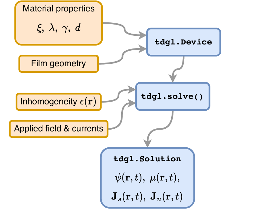
Figure 1: High-level workflow for a pyTDGL simulation. The material properties and geometry of the superconducting film to be modeled are defined by creating an instance of . A instance, along with the applied magnetic vector potential and transport currents, defines a model that can be solved using . Calling returns a instance, which contains the position- and time-dependent simulation results, along with methods for visualization and post-processing.

2 The model

Here we sketch out the generalized time-dependent Ginzburg-Landau model implemented in pyTDGL, and the numerical methods used to solve it. The gTDGL theory is based on Refs. [Kramer1978-kb, Watts-Tobin1981-mn, Jonsson2022-xe, Jonsson2022-mb] and the numerical methods are based on Refs. [Gropp1996-uw, Du1998-kt, Jonsson2022-xe].

The model is applicable to superconducting thin films of arbitrary geometry. By ‘‘thin’’ or ‘‘two-dimensional’’ we mean that the film thickness $d$ is much smaller than the coherence length $\xi=\xi(T)$ and the London penetration depth $\lambda=\lambda(T)$, where $T$ is temperature. This assumption implies that both the superconducting order parameter $\psi(\mathbf{r})$ and the current density $\mathbf{J}(\mathbf{r})$ are roughly constant over the thickness of the film. As described above, the model is strictly speaking valid for temperatures very close to the critical temperature, $T/T_{c}\to 1$, and for dirty superconductors where the inelastic diffusion length much smaller than the coherence length $\xi$ [Kramer1978-kb]. Far below $T_{c}$, GL theory does not correctly describe the physics of the vortex core, but still accurately captures vortex-vortex interactions [Aranson2002-so, Kwok2016-of].

2.1 Time-dependent Ginzburg-Landau

The gTDGL formalism employed here [Kramer1978-kb] consists of a set of coupled partial differential equations for a complex-valued field $\psi(\mathbf{r},t)=|\psi(\mathbf{r},t)|e^{i\theta(\mathbf{r},t)}$ (the superconducting order parameter) and a real-valued field $\mu(\mathbf{r},t)$ (the electric scalar potential) which evolve deterministically in time for a given applied magnetic vector potential $\mathbf{A}_{\mathrm{applied}}(\mathbf{r})$. By default, we assume that Meissner screening is weak, such that the total vector potential in the film is constant in time and equal to the applied vector potential: $\mathbf{A}(\mathbf{r},t)=\mathbf{A}_{\mathrm{applied}}(\mathbf{r})$. The treatment of non-negligible screening is discussed in LABEL:appendix:screening.

In dimensionless units (see Section 2.3), the order parameter $\psi$ evolves according to

$$\begin{split}\frac{u}{\sqrt{1+\gamma^{2}|\psi|^{2}}}&\left(\frac{\partial}{\partial t}+i\mu+\frac{\gamma^{2}}{2}\frac{\partial|\psi|^{2}}{\partial t}\right)\psi\\ &=(\epsilon-|\psi|^{2})\psi+(\nabla-i\mathbf{A})^{2}\psi.\end{split}$$ (1)

The quantity $(\nabla-i\mathbf{A})^{2}\psi$ is the covariant Laplacian of $\psi$, which is used in place of an ordinary Laplacian in order to maintain gauge-invariance. Similarly, $(\frac{\partial}{\partial t}+i\mu)\psi$ is the covariant time derivative of $\psi$. The real-valued parameter $\epsilon(\mathbf{r})=T_{c}(\mathbf{r})/T-1\in[-1,1]$ adjusts the local critical temperature of the film [Kwok2016-of, Al_Luhaibi2022-cl, Sadovskyy2015-ha]. By default, we set $\epsilon(\mathbf{r})=1$. Setting $\epsilon(\mathbf{r})<1$ suppresses the critical temperature at position $\mathbf{r}$, and extended regions of $\epsilon(\mathbf{r})<0$ can be used to model large-scale metallic pinning sites [Kwok2016-of]. The constant $u=\pi^{4}/14\zeta(3)\approx 5.79$ is the ratio of relaxation times for the amplitude and phase of the order parameter in dirty superconductors ($\zeta(x)$ is the Riemann zeta function), and $\gamma$ parameterizes the strength of inelastic scattering as described above. Throughout this work, we assume $\gamma=10$.

The electric potential $\mu(\mathbf{r},t)$ evolves according to the Poisson equation:

$$\begin{split}\nabla^{2}\mu&=\nabla\cdot\mathrm{Im}[\psi^{*}(\nabla-i\mathbf{A})\psi]\\ &=\nabla\cdot\mathbf{J}_{s},\end{split}$$ (2)

where $\mathbf{J}_{s}$ is the dissipationless supercurrent density. The total current density is the sum of the supercurrent density $\mathbf{J}_{s}$ and the normal current density $\mathbf{J}_{n}$:

$$\begin{split}\mathbf{J}&=\mathbf{J}_{s}+\mathbf{J}_{n}\\ &=\mathrm{Im}[\psi^{*}(\nabla-i\mathbf{A})\psi]-\nabla\mu,\end{split}$$ (3)

where $(\nabla-i\mathbf{A})\psi$ and $\psi^{*}$ are the covariant gradient and the complex conjugate of $\psi$, respectively. Eq. 2 results from applying the current continuity equation $\nabla\cdot\mathbf{J}=0$ to Eq. 3:

$$\begin{split}\nabla\cdot\mathbf{J}&=\nabla\cdot(\mathbf{J}_{s}+\mathbf{J}_{n})\\ &=\nabla\cdot\mathrm{Im}[\psi^{*}(\nabla-i\mathbf{A})\psi]-\nabla^{2}\mu\\ &=0.\end{split}$$ (4)

For thin films ($d\ll\lambda$), the thickness-integrated sheet current density is

$$\mathbf{K}=\mathbf{K}_{s}+\mathbf{K}_{n}=d(\mathbf{J}_{s}+\mathbf{J}_{n}).$$ (5)

In addition to the electric potential (Eq. 2), one can couple the dynamics of the order parameter (Eq. 1) to other physical quantities to create a ‘‘multiphysics’’ model. For example, it is common to couple the TDGL equations to the local temperature $T(\mathbf{r},t)$ of the superconductor via a heat balance equation to model self-heating [Gurevich1987-sv, Berdiyorov2012-rn, Zotova2012-nc, Jelic2016-ww, Jing2018-qc].

2.2 Boundary conditions

Isolating boundary conditions are enforced on superconductor-vacuum interfaces, in the form of Neumann boundary conditions for $\psi$ and $\mu$:

$$\hat{\mathbf{n}}\cdot(\nabla-i\mathbf{A})\psi =0$$ (6a)

$$\hat{\mathbf{n}}\cdot\nabla\mu =0,$$ (6b)

where $\hat{\mathbf{n}}$ is a unit vector normal to the interface. Superconductor-normal metal interfaces can be used to apply a bias current density $J_{\mathrm{ext}}$. For such interfaces, we impose Dirichlet boundary conditions on $\psi$ and Neumann boundary conditions on $\mu$:

$$\psi =0$$ (7a)

$$\hat{\mathbf{n}}\cdot\nabla\mu =J_{\mathrm{ext}}.$$ (7b)

A film can have an arbitrary number of normal metal current terminals. If we label the terminals $k=1,2,\ldots$, we can express the global current conservation constraint as

$$\sum_{k}I_{\mathrm{ext},k}=\sum_{k}J_{\mathrm{ext},k}L_{k}=0,$$ (8)

where $I_{\mathrm{ext},k}$ is the total current through terminal $k$, $L_{k}$ is the length of terminal $k$, and $J_{\mathrm{ext},k}$ is the current density along terminal $k$, which we assume to be uniform in magnitude along the terminal and directed normal to the terminal. From Eq. 8, it follows that the current boundary condition for terminal $k$ is:

$$J_{\mathrm{ext},k}=-\frac{1}{L_{k}}\sum_{\ell\neq k}I_{\mathrm{ext},\ell}=-\frac{1}{L_{k}}\sum_{\ell\neq k}J_{\mathrm{ext},\ell}L_{\ell}.$$ (9)

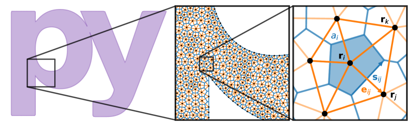
Figure 2: The structure of a finite volume mesh. Left: A superconducting film in the shape of the letters ‘‘py’’. Center: A portion of the finite volume mesh for the film. The mesh sites are shown as black dots, and the triangular Delaunay mesh and dual Voronoi mesh are shown in orange and blue respectively. Right: The mesh site $\mathbf{r}_{i}$ is connected to its nearest neighbors $\mathcal{N}(i)$ by edges $\mathbf{e}_{ij}=\mathbf{r}_{j}-\mathbf{r}_{i}$. Edges (orange lines) that connect three adjacent sites ($i,j,k$) in a counterclockwise fashion form a triangular element $c_{ijk}$ of the Delaunay mesh. The Voronoi region surrounding site $i$ (blue) has an area $a_{i}$, and the edge of the Voronoi cell that intersects edge $\mathbf{e}_{ij}$ has a length $s_{ij}=|\mathbf{s}_{ij}|$. The indexing of mesh sites is arbitrary but fixed.

2.3 Units

The TDGL equations (Eqs. 1 and 2) are solved in dimensionless units, where $\psi$ is measured in units of $|\psi_{0}|$, the magnitude of the order parameter in the absence of applied fields or currents. In these units, we have $0\leq|\psi|^{2}=n_{s}\leq 1$, where $n_{s}$ is the superfluid density normalized to its zero-field value. The scale factors used to convert between physical and dimensionless units are given in terms of material parameters and fundamental constants, namely the superconducting coherence length $\xi$, London penetration depth $\lambda$, normal state conductivity $\sigma$, film thickness $d$, vacuum permeability $\mu_{0}$, and superconducting flux quantum $\Phi_{0}=h/2e$, where $h$ is Planck’s constant and $e>0$ is the elementary charge.

Distance is measured in units of $\xi$. Time is measured in units of

$$\tau_{0}=\mu_{0}\sigma\lambda^{2}.$$

Magnetic field is measured in units of the upper critical field

$$B_{0}=B_{c2}=\mu_{0}H_{c2}=\frac{\Phi_{0}}{2\pi\xi^{2}}.$$

Magnetic vector potential is measured in units of

$$A_{0}=\xi B_{0}=\frac{\Phi_{0}}{2\pi\xi}.$$

Current density is measured in units of

$$J_{0}=\frac{4\xi B_{c2}}{\mu_{0}\lambda^{2}}.$$

Sheet current density is measured in units of

$$K_{0}=J_{0}d=\frac{4\xi B_{c2}}{\mu_{0}\Lambda},$$

where $\Lambda=\lambda^{2}/d$ is the effective magnetic penetration depth. The electric potential $\mu$ is measured in units of

$$V_{0}=\xi J_{0}/\sigma=\frac{4\xi^{2}B_{c2}}{\mu_{0}\sigma\lambda^{2}}.$$

3 Numerical implementation

3.1 Finite volume method

To simulate superconducting films of any shape, we solve the TDGL model on an unstructured Delaunay mesh in two dimensions [Du1998-kt, Jonsson2022-xe], as illustrated in Figure 2. The mesh is composed of a set of sites, each denoted by its position $\mathbf{r}_{i}\in\mathbb{R}^{2}$ or an integer index $i$, and a set of triangular cells $c_{ijk}$. Nearest-neighbor sites $\mathbf{r}_{i}$ and $\mathbf{r}_{j}$ are connected by an edge, denoted by the vector $\mathbf{e}_{ij}=\mathbf{r}_{j}-\mathbf{r}_{i}$ or the 2-tuple $(i,j)$, which has a length $e_{ij}=|\mathbf{e}_{ij}|$ and a direction $\hat{\mathbf{e}}_{ij}=\mathbf{e}_{ij}/e_{ij}$. Each cell $c_{ijk}=(i,j,k)$ represents a triangle with three edges ($(i,j)$, $(j,k)$, and $(k,i)$) that connect sites $\mathbf{r}_{i}$, $\mathbf{r}_{j}$, $\mathbf{r}_{k}$ in a counterclockwise fashion. Each site is assigned an effective area $a_{i}$, which is the area of the Voronoi cell surrounding the site. The Voronoi cell surrounding site $i$ consists of all points in $\mathbb{R}^{2}$ that are closer to site $\mathbf{r}_{i}$ than to any other site in the mesh. The side of the Voronoi cell that intersects edge $(i,j)$ is denoted $\mathbf{s}_{ij}$ and has a length $s_{ij}$. The collection of all Voronoi cells tessellates the film and forms a mesh that is dual to the triangular Delaunay mesh.

A scalar function $f(\mathbf{r},t)$ can be discretized at a given time $t^{n}$ as the value of the function on each site, $f_{i}^{n}=f(\mathbf{r}_{i},t^{n})$. A vector function $\mathbf{F}(\mathbf{r},t)$ can be discretized at time $t^{n}$ as the flow of the vector field between sites, $F_{ij}^{n}=\mathbf{F}((\mathbf{r}_{i}+\mathbf{r}_{j})/2,t^{n})\cdot\hat{\mathbf{e}}_{ij}$, where $(\mathbf{r}_{i}+\mathbf{r}_{j})/2=\mathbf{r}_{ij}$ is the center of edge $(i,j)$. The gradient of a scalar function $g(\mathbf{r})$ is approximated on the edges of the mesh. The value of $\nabla g$ at position $\mathbf{r}_{ij}$ is:

$$(\nabla g)_{ij}=\left.(\nabla g)\right|_{\mathbf{r}_{ij}}\approx\frac{g_{j}-g_{i}}{e_{ij}}\hat{\mathbf{e}}_{ij}.$$ (10)

To calculate the divergence of a vector field $\mathbf{F}(\mathbf{r})$ on the mesh, we assume that each Voronoi cell is small enough that the value of $\nabla\cdot\mathbf{F}$ is constant over the area of the cell and equal to the value at the mesh site lying inside the cell, $\mathbf{r}_{i}$. Then, using the divergence theorem in two dimensions, we have

$$\begin{split}\int(\nabla\cdot\mathbf{F})\,\mathrm{d}^{2}\mathbf{r}&=\oint(\mathbf{F}\cdot\hat{\mathbf{n}})\,\mathrm{d}s\\ \left.(\nabla\cdot\mathbf{F})a_{i}\right|_{\mathbf{r}_{i}}&\approx\sum_{j\in\mathcal{N}(i)}F_{ij}s_{ij}\\ (\nabla\cdot\mathbf{F})_{i}=\left.(\nabla\cdot\mathbf{F})\right|_{\mathbf{r}_{i}}&\approx\frac{1}{a_{i}}\sum_{j\in\mathcal{N}(i)}F_{ij}s_{ij},\end{split}$$ (11)

where $\mathcal{N}(i)$ is the set of sites adjacent to site $\mathbf{r}_{i}$. The Laplacian of a scalar function $g$ is given by $\nabla^{2}g=\nabla\cdot\nabla g$, so combining Eqs. 10 and 11 we have

$$(\nabla^{2}g)_{i}=\left.(\nabla^{2}g)\right|_{\mathbf{r}_{i}}\approx\frac{1}{a_{i}}\sum_{j\in\mathcal{N}(i)}\frac{g_{j}-g_{i}}{e_{ij}}s_{ij}.$$ (12)

The discrete gradient, divergence, and Laplacian of a field at site $i$ depend only on the value of the field at site $i$ and its nearest neighbors. This means that the corresponding operators, Eqs. 10, 11, and 12, can be efficiently represented as sparse matrices, and their action given by sparse matrix-vector products.

3.2 Covariant derivatives

We use link variables to construct covariant versions of the spatial derivatives and time derivatives of $\psi$ [Gropp1996-uw, Du1998-kt, Du1998-rb]. In the discrete case corresponding to our finite volume method, this amounts to adding a complex phase whenever taking a difference in $\psi$ between mesh sites (for spatial derivatives) or time steps (for time derivatives).

The covariant gradient of $\psi$ at time $t^{n}$ and edge $\mathbf{r}_{ij}$ is:

$$\left.\left(\nabla-i\mathbf{A}\right)\psi\right|_{\mathbf{r}_{ij}}^{t^{n}}=\frac{U^{n}_{ij}\psi_{j}^{n}-\psi_{i}^{n}}{e_{ij}}\hat{\mathbf{e}}_{ij},$$ (13)

where $U^{n}_{ij}=\exp(-i\mathbf{A}(\mathbf{r}_{ij},t^{n})\cdot\mathbf{e}_{ij})$ is the spatial link variable. Eq. 13 is similar to the gauge-invariant phase difference in Josephson junction physics. The covariant Laplacian of $\psi$ at time $t^{n}$ and site $\mathbf{r}_{i}$ is:

$$\left.\left(\nabla-i\mathbf{A}\right)^{2}\psi\right|_{\mathbf{r}_{i}}^{t^{n}}=\frac{1}{a_{i}}\sum_{j\in\mathcal{N}(i)}\frac{U^{n}_{ij}\psi_{j}^{n}-\psi_{i}^{n}}{e_{ij}}s_{ij}$$ (14)

The covariant time derivative of $\psi$ at time $t^{n}$ and site $\mathbf{r}_{i}$ is

$$\left.\left(\frac{\partial}{\partial t}+i\mu\right)\psi\right|_{\mathbf{r}_{i}}^{t^{n}}=\frac{U_{i}^{n,n+1}\psi_{i}^{n+1}-\psi_{i}^{n}}{\Delta t^{n}},$$ (15)

where $U_{i}^{n,n+1}=\exp(i\mu_{i}^{n}\Delta t^{n})$ is the temporal link variable.

3.3 Euler method

The discretized form of the equations of motion for $\psi(\mathbf{r},t)$ (Eq. 1) and $\mu(\mathbf{r},t)$ (Eq. 2) are:

$$\begin{split}&\frac{u}{\Delta t^{n}\sqrt{1+\gamma^{2}\left|\psi_{i}^{n}\right|^{2}}}\left[\psi_{i}^{n+1}e^{i\mu_{i}^{n}\Delta t^{n}}-\psi_{i}^{n}+\frac{\gamma^{2}}{2}\left(\left|\psi_{i}^{n+1}\right|^{2}-\left|\psi_{i}^{n}\right|^{2}\right)\psi_{i}^{n}\right]\\ &\quad=\left(\epsilon_{i}-\left|\psi_{i}^{n}\right|^{2}\right)\psi_{i}^{n}+\frac{1}{a_{i}}\sum_{j\in\mathcal{N}(i)}\frac{U^{n}_{ij}\psi_{j}^{n}-\psi_{i}^{n}}{e_{ij}}s_{ij}\end{split}$$ (16)

and

$$\begin{split}\sum_{j\in\mathcal{N}(i)}\frac{\mu_{j}^{n}-\mu_{i}^{n}}{e_{ij}}s_{ij}&=\sum_{j\in\mathcal{N}(i)}J_{s,ij}^{n}|s_{ij}|\end{split}$$ (17)

respectively, where supercurrent $J_{ij}^{n}$ is given by

$$J^{n}_{s,ij}=\mathrm{Im}\left\{\left(\psi_{i}^{n}\right)^{*}\,\frac{U^{n}_{ij}\psi_{j}^{n}-\psi_{i}^{n}}{e_{ij}}\right\}.$$ (18)

The superscript $n$ is an integer index denoting the solve step or iteration and $\Delta t^{n}$ is the time step in units of $\tau_{0}$. If we isolate the terms in Eq. 16 involving the order parameter at time $t^{n+1}$, we can rewrite Eq. 16 in the form

$$\psi_{i}^{n+1}+z_{i}^{n}\left|\psi_{i}^{n+1}\right|^{2}=w_{i}^{n},$$ (19)

where

$$z_{i}^{n}=\frac{\gamma^{2}}{2}e^{-i\mu_{i}^{n}\Delta t^{n}}\psi_{i}^{n}$$ (20)

and

$$\begin{split}w_{i}^{n}=&z_{i}^{n}\left|\psi_{i}^{n}\right|^{2}+e^{-i\mu_{i}^{n}\Delta t^{n}}\,\times\\ &\Biggl{[}\psi_{i}^{n}+\frac{\Delta t^{n}}{u}\sqrt{1+\gamma^{2}\left|\psi_{i}^{n}\right|^{2}}\,\times\\ &\quad\biggl{(}\left(\epsilon_{i}-\left|\psi_{i}^{n}\right|^{2}\right)\psi_{i}^{n}+\frac{1}{a_{i}}\sum_{j\in\mathcal{N}(i)}\frac{U^{n}_{ij}\psi_{j}^{n}-\psi_{i}^{n}}{e_{ij}}s_{ij}\biggr{)}\Biggr{]}.\end{split}$$ (21)

Solving Eq. 19 for $\left|\psi_{i}^{n+1}\right|^{2}$, we arrive at a quadratic equation in $\left|\psi_{i}^{n+1}\right|^{2}$:

$$\left|z_{i}^{n}\right|^{2}\left|\psi_{i}^{n+1}\right|^{4}-(2c_{i}^{n}+1)\left|\psi_{i}^{n+1}\right|^{2}+\left|w_{i}^{n}\right|^{2}=0,$$ (22)

where we have defined

$$c_{i}^{n}=\mathrm{Re}\left\{z_{i}^{n}\right\}\mathrm{Re}\left\{w_{i}^{n}\right\}+\mathrm{Im}\left\{z_{i}^{n}\right\}\mathrm{Im}\left\{w_{i}^{n}\right\}.$$ (23)

See LABEL:appendix:euler for an explicit derivation of Eq. 22. To solve Eq. 22, which has the form $ax^{2}+bx+c=0$, we use a modified quadratic formula:

$$\begin{split}x&=\frac{-b\pm\sqrt{b^{2}-4ac}}{2a}\cdot\frac{-b\mp\sqrt{b^{2}-4ac}}{-b\mp\sqrt{b^{2}-4ac}}\\ &=\frac{2c}{-b\mp\sqrt{b^{2}-4ac}}\end{split}$$ (24)

in order to avoid numerical issues when $a=\left|z_{i}^{n}\right|^{2}=0$, i.e., when $\left|\psi_{i}^{n}\right|^{2}=0$ or $\gamma=0$. Applying Eq. 24 to Eq. 19 yields

$$\left|\psi_{i}^{n+1}\right|^{2}=\frac{2\left|w_{i}^{n}\right|^{2}}{(2c_{i}^{n}+1)+\sqrt{(2c_{i}^{n}+1)^{2}-4\left|z_{i}^{n}\right|^{2}\left|w_{i}^{n}\right|^{2}}}.$$ (25)

We take the root with the ‘‘$+$’’ sign in Eq. 25 because the ‘‘$-$’’ sign results in unphysical behavior where $\left|\psi_{i}^{n+1}\right|^{2}$ diverges when $\left|z_{i}^{n}\right|^{2}$ vanishes (i.e., when $\left|\psi_{i}^{n}\right|^{2}$ and/or $\gamma$ is zero).

Combining Eq. 19 and Eq. 25 allows us to find the order parameter at time $t^{n+1}$ in terms of the order parameter and the electric potential at time $t^{n}$:

$$\begin{split}\psi_{i}^{n+1}&=w_{i}^{n}-z_{i}^{n}\left|\psi_{i}^{n+1}\right|^{2}\\ &=w_{i}^{n}-z_{i}^{n}\frac{2\left|w_{i}^{n}\right|^{2}}{(2c_{i}^{n}+1)+\sqrt{(2c_{i}^{n}+1)^{2}-4\left|z_{i}^{n}\right|^{2}\left|w_{i}^{n}\right|^{2}}}.\end{split}$$ (26)

Combining Eq. 26 and Eq. 17 yields a sparse linear system that can be solved to find $\mu_{i}^{n+1}$ given $\mu_{i}^{n}$ and $\psi_{i}^{n+1}$. Eq. 17 is solved using sparse LU decomposition [Li2005-gv].

3.4 Adaptive time step

pyTDGL uses an adaptive time step algorithm that adjusts the time step $\Delta t^{n}$ based on the speed of the system’s dynamics, which can significantly reduce the wall-clock time of a simulation without sacrificing solution accuracy (See LABEL:appendix:adpative). There are three parameters that control the adaptive time step algorithm, $\Delta t_{\mathrm{init}}$, $\Delta t_{\mathrm{max}}$, and $N_{\mathrm{window}}$. The initial time step in iteration $n=0$ is set to $\Delta t^{0}=\Delta t_{\mathrm{init}}$. We keep a running list of $\Delta|\psi|^{2}_{n}=\max_{i}\left|\left(\left|\psi_{i}^{n}\right|^{2}-\left|\psi_{i}^{n-1}\right|^{2}\right)\right|$ for each iteration $n$. Then, for each iteration $n>N_{\mathrm{window}}$, we define a tentative new time step $\Delta t_{\star}$ using the following heuristic:

$$\delta_{n} =\frac{1}{N_{\mathrm{window}}}\sum_{\ell=0}^{N_{\mathrm{window}}-1}\Delta|\psi|^{2}_{n-\ell}$$ (27a)

$$\Delta t_{\star} =\min\left(\frac{1}{2}\left(\Delta t^{n}+\frac{\Delta t_{\mathrm{init}}}{\delta_{n}}\right),\;\Delta t_{\mathrm{max}}\right)$$ (27b)

Eq. 27 has the effect of automatically selecting a small time step if the recent dynamics of the order parameter are fast (i.e., if $\delta_{n}$ is large) and a larger time step if the dynamics are slow. The the tentative time step selected at solve step $n$ may be too large to accurately solve for the state of the system in step $m=n+1$. We detect such a failure to converge by evaluating the discriminant of Eq. 22. If the discriminant, $(2c_{i}^{m}+1)^{2}-4|z_{i}^{m}|^{2}|w_{i}^{m}|^{2}$, is less than zero for any site $i$, then the value of $|\psi_{i}^{m+1}|^{2}$ found in Eq. 25 will be complex, which is unphysical. If this happens, we iteratively reduce the time step $\Delta t^{m}$ (setting $\Delta t^{m}\leftarrow\Delta t^{m}\times M_{\mathrm{adaptive}}$ at each iteration, where $0<M_{\mathrm{adaptive}}<1$ is a user-defined multiplier) and re-solve Eq. 22 until the discriminant is nonnegative for all sites $i$, then proceed with the rest of the calculation for step $m$. If this process fails to find a suitable $\Delta t^{m}$ in $N_{\mathrm{retries}}^{\mathrm{max}}$ iterations, where $N_{\mathrm{retries}}^{\mathrm{max}}$ is a parameter that can be set by the user, the solver raises an error. Pseudocode for the main solver is given in Algorithms LABEL:alg:adaptive-euler-step and LABEL:alg:adaptive in LABEL:appendix:pseudocode.

4 Package overview

In this section, we provide an overview of the pyTDGL Python package. The package is written for and tested on Python versions 3.8, 3.9, and 3.10. The numerical methods described in Section 3 are implemented using NumPy [Harris2020-xv] and SciPy [Virtanen2020-zz], data visualization is implemented using Matplotlib [Hunter2007-il], and data storage is implemented using the HDF5 file format via the h5py library [Collette2013-rq]. Physical units are managed using Pint [Grecco], and finite element meshes are generated using the MeshPy [Klockner] Python interface to Triangle [Shewchuk1996-va], a fast compiled 2D mesh generator. The pyTDGL Python user interface is adapted from SuperScreen [Bishop-Van_Horn2022-sy], and some of the finite volume and interactive visualization code is adapted from SuperDetectorPy, a public GitHub repository accompanying Refs. [Jonsson2022-xe, Jonsson2022-mb].

pyTDGL is hosted on GitHub, and automated testing is performed using the GitHub Actions continuous integration (CI) tool. The package can be installed from GitHub or PyPI, the Python Package Index. The source code and online documentation are provided under the MIT License. The stable version of the package corresponding to this manuscript is v0.2.1.

4.1 Device interface

The material properties and geometry of a superconducting device to be modeled are defined by creating an instance of the sec:units. A tdgl.Layer and one or more Layer stores the coherence length $\xi$, London penetration depth $\lambda$, inelastic scattering parameter $\gamma$, and film thickness $d$. Instances of Polygons can be manipulated using affine transformations (translation, scaling, rotation) and combined using constructive solid geometry methods (see Table LABEL:table:polygon) to generate complex shapes from simple geometric primitives such as rectangles and ellipses . One can also define any number of ‘‘probe points,’’ which are positions $\mathbf{r}_{p,i}$ in the film for which the electric potential $\mu(\mathbf{r}_{p,i},t^{n})$ and phase $\theta(\mathbf{r}_{p,i},t^{n})=\arg\psi(\mathbf{r}_{p,i},t^{n})$ are measured at each solve step $n$.

A.difference(B)