Toward a Theory of Causation for Interpreting Neural Code Models

Abstract

Neural Language Models of Code, or Neural Code Models (NCMs), are rapidly progressing from research prototypes to commercial developer tools. As such, understanding the capabilities and limitations of such models is becoming critical. However, the abilities of these models are typically measured using automated metrics that often only reveal a portion of their real-world performance. While, in general, the performance of NCMs appears promising, currently much is unknown about how such models arrive at decisions. To this end, this paper introduces do_code, a post-hoc interpretability methodology specific to NCMs that is capable of explaining model predictions. do_code is based upon causal inference to enable programming language-oriented explanations. While the theoretical underpinnings of do_code are extensible to exploring different model properties, we provide a concrete instantiation that aims to mitigate the impact of spurious correlations by grounding explanations of model behavior in properties of programming languages. To demonstrate the practical benefit of do_code, we illustrate the insights that our framework can provide by performing a case study on two popular deep learning architectures and nine NCMs. The results of this case study illustrate that our studied NCMs are sensitive to changes in code syntax and statistically learn to predict tokens related to blocks of code (e.g., brackets, parenthesis, semicolon) with less confounding bias as compared to other programming language constructs. These insights demonstrate the potential of do_code as a useful model debugging mechanism that may aid in discovering biases and limitations in NCMs.

I Introduction

The combination of large amounts of freely available code-related data, which can be mined from open source repositories, and ever-more sophisticated architectures for Neural Language Models of Code, which we refer to as Neural Code Models (NCMs) in this paper, have fueled the development of Software Engineering (SE) tools with increasing effectiveness. NCMs have (seemingly) illustrated promising performance across a range of different SE tasks [1, 2, 3, 4]. In particular, code generation has been an important area of SE research for decades, enabling tools for downstream tasks such as code completion [5], program repair [6], and test case generation [1]. In addition, industry interest in leveraging NCMs for code generation has also grown as evidenced by tools such as Microsoft’s IntelliCode [7], Tabnine [8], OpenAI’s Codex [9], and GitHub’s Copilot [10]. Given the prior popularity of code completion engines within IDEs [11], and the pending introduction of, and investment in commercial tools, NCMs for code generation will almost certainly be used to help build production software systems in the near future, if they are not being used already.

However, it is generally accepted that Neural Language Models operate in a black-box fashion. That is, we are uncertain how these models arrive at decisions, which is why NCMs suffer from incompleteness in problem formalization [12]. As such, much of the work on NCMs has primarily relied upon automated metrics (e.g., Accuracy, BLEU, METEOR, ROUGE) as an evaluation standard. Skepticism within the natural language processing (NLP) research community is growing regarding the efficacy of current automated metrics  [13, 14, 15], as they tend to overestimate model performance. Even benchmarks that span multiple tasks and metrics have been shown to lack robustness, leading to incorrect assumptions of model comparisons [16].

Despite the increasing popularity and apparent effectiveness of neural code generation tools, there is still much that is unknown regarding the practical performance of these models, their ability to learn and predict different code-related concepts, and their current limitations. Some of the most popular models for code generation have been adapted from the field of NLP, and thus may inherit the various limitations often associated with such models — including biases, memorization, and issues with data inefficiency, to name a few [17]. In fact, recent work from Chen et al. [18] illustrates that certain issues, such as alignment failures and biases, do exist for large-scale NCMs. Most of the conclusions from Chen et al.’s study were uncovered through manual analysis, e.g., through sourcing counterexamples, making it difficult to rigorously quantify or to systematically apply such an analysis to research prototypes [19]. Given the rising profile and role that NCMs for code generation play in SE, and the current limitations of adopted evaluation techniques, it is clear that new methods are needed that provide deeper insight into NCMs’ performance. Notable work has called for a more systematic approach [13] that aims to understand a given model’s behavior according to its linguistic capabilities and tests customized for the given task for which a model is applied.

As the discussion above suggests, while it may appear that NCMs have begun to achieve promising performance, it is clearly insufficient to examine only prediction values (i.e., the what of NCMs’ decision). This current status quo, at best, provides an incomplete picture of the limitations and caveats of NCMs for code. Given the potential impact and consequence of these models and their resulting applications, there is a clear need to strive for a more complete understanding of how they function in practice. As such, we must push to understand how NCMs arrive at their predictions (i.e., the why of NCMs’ decision). In this paper, we cast this problem of achieving a more complete understanding of Neural Code Models as an Interpretable Machine Learning task and posit that we can leverage the theory of causation as a mechanism to explain NCMs prediction performance. We hypothesize that this mechanism can serve as a useful debugging tool for detecting biases, understanding limitations, and eventually, increasing the reliability and robustness of NCMs employed for the task of code generation [20, 12].

This paper introduces do_code, a novel post-hoc interpretability method specifically designed for understanding the effectiveness of NCMs. The intention of do_code is to establish a robust and adaptable methodology for interpreting predictions of NCMs trained on code in contrast to simply measuring the accuracy of these same NCMs. More specifically, do_code consists of two major conceptual components, (i) a structural causal graph, and (ii) a causal inference mechanism. do_code’s structural causal graph maps model predictions to programming language (PL) concepts and variations in test datasets at different levels of granularity, thus enabling statistical analyses of model predictions rooted in understandable concepts. While our methodology allows for extensiblility in defining relevant PL concepts, we offer an initial code taxonomy as a generalizable example. However, examining statistical properties of model predictions in isolation does not provide explanations regarding observed performance. As such, the second theoretical component of do_code adopts a causal understanding mechanism that can explain observed trends in model predictions rooted in the aforementioned programming language concepts. This causal inference mechanism allows for the generation of explanations of model performance rooted in do_code’s understandable concepts. Through the introduction of this interpretability framework, we aim to help SE researchers and practitioners by allowing them to understand the potential limitations of a given model, work towards improving models and datasets based on these limitations, and ultimately make more informed decisions about how to build automated developer tools given a more holistic understanding of what NCMs are predicting and why the predictions are being made.

To showcase the types of insights that do_code can uncover, we perform a case study (see Sec. V) on different variations of two popular deep learning architectures for the task of code generation, namely RNNs [21] and Transformers [22] trained on the CodeSearchNet dataset [23]. We instantiated our study using ten structural code categories derived from the Java programming language. This case study resulted in several notable findings illustrating the efficacy of our interpretability technique: (i) we find that our studied models learn to predict tokens related to code blocks (e.g., brackets, parentheses, semicolons) more effectively than most other code token types (e.g., loops, conditionals, datatypes), (ii) we found that our studied models are sensitive to seemingly subtle changes in code syntax, reinforcing previous studies concluding the same [24], and (iii) our studied models are only marginally impacted by the presence of comments and bugs, which challenges findings from previous work [25].

We hope to provide researchers a way forward for integrating causal analysis into their research. To that end, besides our case study showing the power of such an analysis can provide, we have additionally created a checklist that summarizes the steps required to apply Causal Interpretability to Neural Code Models (see Fig. 7). In summary, this paper makes the following contributions:

1. A formal methodology for interpreting NCMs that maps model performance to PL concepts and enables causal analyses of different settings for language model use;

2. A case study that applies this methodology to two popular deep learning code generation models;

3. A set of findings for these models that challenges some current conceptions of code generation models;

4. A checklist to help research apply Causal Interpretability to Neural Code Models;

5. And a replication package[26] to both encourage the use of our technique in future work on developing and evaluating code generation models and for replicating our experiments.

II An Overview of the do_code Approach

do_code comprises a set of statistical and causal inference methods to interpret the global and local prediction performance of NCMs for code. In the simplest of terms, our proposed methodology asks Why does a NCM make a given prediction? – and provides a framework for answering this broad question by (i) mapping code tokens to higher level PL/SE concepts, (ii) examining how well models predict tokens mapped to these concepts across different settings (e.g., predicting code with and without comments), and (iii) using a structural causal model to derive explanations that take into consideration potential confounding factors (e.g., method size, code duplication). do_code is a posthoc interpretability technique (i.e., after models have been trained) and hence is generally agnostic to the specifics of the model architecture to which it is being applied, making it highly extensible.

Below, we provide a high level explanation of how each component of do_code functions before describing the formalism and process in detail in Sections III & IV.

II-A Component 1: Mapping Source Code Tokens to SE/PL Concepts

To help bridge the gap between a given NCMs abstract representation of code and human-understandable concepts, the first component of do_code aims to map well-known concepts from programming languages to individual tokens.

II-A1 Structural Code Taxonomy

Source code tokens can be mapped to any number of PL/SE concepts, and for our implementation of do_code, we focus on mapping tokens to different implicit syntactic groups, which do not require manual labeling of concepts. This mitigates the cost involved with large-scale data labeling, and still provides explanations rooted in concepts with which most programmers and researchers are likely familiar. In PLs, different types of tokens retain different semantic meanings. For instance ‘=’ and ‘<’ are common operators. As such, we can group tokens into semantically meaningful categories. These categories serve as features that allow do_code to assign semantic meaning to predicted tokens. The taxonomy comprises high-level properties of code using a mapping function $\phi_{\mathcal{H}}:w\to h$, where $w$ corresponds to tokens of the model vocabulary $\mathcal{V}$ and each token in a sequence $w$ is assigned to a human understandable concept $h$ (i.e., our defined categories). We introduce a taxonomy and mapping function for Java code tokens in detail in Sec. IV. Note that do_code can work with any mapping function, not only the one we define, making it easily extensible for performing other types of analyses a researcher might be interested in.

II-B Component 2: Defining Structural Causal Model

While our source code token mapping provides the building blocks for explaining global model behavior when applied to predict different types of software data, it may be difficult to determine whether any correlations in performance are causal, i.e., definitely resulting from the intervention, or spurious, i.e., potentially caused by confounding factors. To enable an analysis of whether a change in model performance is truly causal or not, allowing for the generation of accurate explanations, we propose an analysis based on causal inference which we describe below.

II-B1 Causation and Structural Causal Models

A variable $T$ is a cause of $Y$ if the variable $Y$ depends on $T$ to determine its value. However, there are also variables $U$ that represent unmodeled factors [27]. This causal relationship can be precisely formulated via a causal model that uses directed acyclic graphs (DAGs) to describe direct parent-child relationships, instead of probabilistic dependencies, among random variables such as $T$ and $Y$. It also allows us to introduce a graphical definition of causation [27, 28].

Structural Causal Models (SCMs) are stable mechanisms that remain invariant to local changes unlike probabilities computed by Bayesian networks [29]. This characteristic is responsible for enabling us to quantitatively estimate the results of an action or intervention in the graph. In other words, SCMs provide a framework for counterfactual reasoning.

II-B2 Code Corpora Interventions

In order to enable our analysis based upon SCMs, we need to design interventions, or changes in the data distribution that represent a meaningful concept (i.e., commented vs. uncommented), in order to attribute cause from the changes in the model’s performance in predicting the SE/PL concepts defined in the previous subsection. That is, if we observe that a model is less effective at predicting operators after changing “test” data sequences to which the model is applied, we can say that the change caused this drop in effectiveness, if we properly control for confounding factors. We design do_code’s interventions based on the fact that NCMs are often not applied to the same types of code corpora upon which they are trained. For instance, if a model trained on a well-commented dataset is applied to predict segments of poorly commented code, this could potentially impact performance. As such we define parallel code corpora which contain SE/PL specific changes across the datasets, and specifically introduce four different initial interventions described in the next component (see Sec. II-C).

II-B3 Confounding Factors for Global Explanations

In past work several factors, such as code duplication [30], have been illustrated to affect model predictions. As such, we derive a list of potential confounding factors that could influence a model’s prediction of our mapped PL/SE concepts beyond our interventions defined in the previous section. Our initial set of factors (also called covariates) include, McCabe’s complexity, LoC (Lines of code), number of {returns, loops, comparisons, try/catches, parenthesized expressions, Number, String literals, Variables, Max nested blocks, anonymous classes, inner classes, and lambda expressions}, and number of {unique words, log statements, modifiers} in a method.

II-C Component 3: Connecting Structural Causal Models with Code Corpora

We define Code Corpora Interventions to better understand model performance across different settings. We formulate these settings as parallel code corpora with differing specified semantic properties. For instance, a testbed oriented to simulate a debugging environment, may consist of two parallel corpora: the buggy code, and the (corresponding) fixed code. Therefore, these datasets describe some high-level SE property, which we employ in do_code’s causal analysis. We define four types of SE application settings, adapted from both our prior work and community datasets: (i) buggy/non-buggy [31], (ii) commented/non-commented [32], (iii) type II, and (iv) type III clone pairs [33]. do_code is extensible, meaning that researchers can define their own code corpora interventions. In addition, we have also defined Model Hyper-parameter Interventions to extend the causal analysis beyond data or code corpora perturbations (see Sec. IV-B).

II-C1 An Example Application of our Causal Analysis

Consider the scenario in which we want to understand how a given model operates between buggy and fixed code. To do this do_code constructs a SCM composed of an intervention variable $T=Buggy$ and potential outcome $Y=Perf$ (representing a measure of model effectiveness or performance in terms of our defined code concepts). In addition, we identify confounding factors (or the covariates from the previous subsection) $Z$ for interventions and potential outcomes. Next we want to perform the intervention wherein the model is applied to fixed code instead of buggy code. do_code then constructs a parallel graph for this intervention. Using concepts from causal inference theory, do_code is then able to determine how the intervention affected model performance in terms of code concepts, and whether the change in performance is a true causal effect, or spurious, resulting from effects of covariates.

II-D Component 4: Enabling Causal Interpretability for NCMs

If we want to estimate how our buggy/non-buggy code corpora intervention- in the previous example application- affects the performance of a NCM, we just need to estimate the effect of the treatment using the adjustment formula of causal inference (see Def. 3).

II-D1 Measuring Causal Effects & Generating Explanations

While the above explanations and example illustrate the intuition of our causal analysis, it is important to define how causal effects, and ultimately explanations, will be generated. First, we need methods by which we can measure model performance. To do this we use Cross-Entropy loss, or the difference in distribution of the model’s prediction and the ground-truth for given token sequences, and average Next Token Predictions, or probabilities assigned by models to individual tokens, across token sequences as these measures are relevant values produced at inference time that reflect the prediction effectiveness. By relating these values to counterfactual interventions $T$ (i.e., buggy/non-buggy intervention), we can gain an understanding of how well a studied model is generating code under these treatments. To calculate causal effects for binary treatments similar to the ones we used in $T_{[data]}$ (e.g., Buggy/Fixed, Commented/Uncommented, and Clone1/Clone2), we first calculate association correlations (Def. 5) and then causal effects (Def. 6). After the causal effect is calculated, we aim to generate natural language explanations from our analysis via structured templates that relate code token concepts to the intervention: e.g., [code token concept] performed worse by [change in performance], due to a change in model application from [intervention] to [intervention], with a causal analysis ATE of [ATE value].

II-E Component 5: Evaluating Causal Effects

An important step in causal analysis is the validation of our causal estimates. In order to perform this validation, we employ refutation methods that calculate the robustness of the causal estimate. These methods test the robustness of our assumptions through various types of perturbations to see the impact on our $ATE$ estimation. There are multiple refutation methods, but in this paper, we focus on four: adding a random common cause or covariate $\mathcal{R}_{1}$, adding an unobserved common cause or covariate $\mathcal{R}_{2}$, replacing the treatment with a random variable or placebo $\mathcal{R}_{3}$, and removing a random subset of the data $\mathcal{R}_{4}$. Depending on the method, the resulting value should either be the same as the original $ATE$ or close to zero.

III Formalizing Causal Interpretability for Neural Code Models

In this section, we introduce formalism related to some of the concepts of causal inference used by do_code. The ultimate goal of interpretability in Deep Learning for Software Engineering (DL4SE) is to generate explanations of Neural Code Models’ decisions represented as prediction performance (i.e., Cross-Entropy or Next Token Prediction). A method to generate these explanations is based on the idea of estimating the effect of interventions on the inputs or parameters that configure NCMs.

Example 1

Consider a Bayesian network created to explain the performance of a given NCM, represented as an arrow that links buggy input code to model performance $Buggy\to Perf$. The variables $Buggy$ and $Perf$ are dependent, both variables embody a program repair intervention. Therefore, if we want to define the joint distribution $p(Buggy,Perf)$ to represent the network, we must specify by Bayes’ rule using the prior $p(Buggy)$ and the conditional probability $p(Perf|Buggy)$. Nonetheless, such a joint distribution can be computed as well in the opposite direction $Perf\to Buggy$ using the same Bayes’ rule for a prior $p(Perf)$ and conditional $p(Buggy|Perf)$. The fact that the joint distribution can be represented with both networks is non-intuitive since we know from experience and software understanding that the model performance cannot give rise to a bug in the original input. In other words, the relationship between these variables is asymmetric or causal. Hence, we expect that buggy snippets affect the performance of NCMs, not the other way around.

A first attempt to address the relationship in Ex. 1 would be computing a correlation coefficient $\rho_{TY}\approx p(Y|T)=p(Perf|Buggy)$, where $T$ is a binary treatment that represents the debugging process and $Y$ is a potential outcome that corresponds to the model performance. This coefficient, however, is still symmetric: if $T$ is correlated with $Y$, then $Y$ is equally correlated with $T$. Causal networks allow us to model causal asymmetries where directionality goes beyond probabilistic dependence. These causal models represent the mechanism by which data were generated [29]. Instead of testing whether $Buggy$ and $Perf$ are conditionally dependent, causation asks which variable responds to the other one: $Buggy$ to $Perf$ or $Perf$ to $Buggy$? [29].

Definition 1

Causation. A variable $T$ is a cause of $Y$ if the variable $Y$ depends on $T$ to determine its value. Formally, the value of $Y$ was assigned on the basis of what it is known about $T$. In other words, the value of $Y$ is determined by a structural equation $Y=f_{y}(T,U_{y})$ and the arrow $T\to Y$. The $U$ variables in these equations represent unmodeled variables that are exogenous to the causal network but disturb the functional relationship between the outcome and its treatment [27].

Similarly, we can define a structural function for the treatment $T=f_{t}(U_{t})$ that depends only on $U$ disturbances assuming that no common causes exists between outcomes and treatments. A common cause is a random variable $Z$ that causally influence two variables that are initially perceived as statically dependant ($T\not\!\perp\!\!\!\perp Y$). However, this dependency can be explained by the underlying influence of $Z$ on the effects, making the effects in fact conditionally independent ($T\perp\!\!\!\perp Y|Z$). Therefore, there exist more complex causal relationships between treatments and outcomes that we are able to model with structural equations that corresponds to a Structural Causal Model (SCM).

Definition 2

Structural Causal Models. These directed acyclic graphs (DAGs) describe direct parent-child relationships, instead of probabilistic dependencies, among random variables $X_{i}$. The value $x_{i}$ of each variable $X_{i}$ is defined by the structural equations $x_{i}=f_{i}(PA_{i},U_{i})$ where $PA_{i}={X_{j}:X_{j}\to X_{i}}$ denotes the set of parents or direct causes of $X_{i}$. This model allow us to introduce a graphical definition of causation [27, 28].

SCMs are stable mechanisms that remain invariant to local changes unlike probabilities computed by Bayesian networks [29]. This characteristic is responsible for enabling us to estimate quantitatively the results of an action or intervention in the graph without actually performing it in controlled settings (i.e., randomized experiments). In other words, SCMs provide a framework for counterfactual reasoning. The mathematical tool employed to perform these interventions is the $do(\cdot)-operator$ [28]. For instance, if we want to estimate how fixed code affects the performance of a NCM, we just need to compute the action $p(Perf|do(Buggy=False))$ (Eq. 1a). These type of actions are interventional distributions since we set the value of $Buggy$ to $False$. Note that this interventional distribution is not necessarily $p(Perf|Buggy=False)$ (Eq. 1b). This latter distribution is observational since we are conditioning the performance on the value of the $Buggy$ variable. Intervening on a variable in a SCM means fixing its value and, therefore, changing the value of other variables of the network as a result. Conversely, conditioning on a variable means narrowing the cases that the outcome takes once we assign a value to the treatment.

Figure 1: (a) Structural Causal Model representing cause-effect relationships of program repair in NCMs. (b) The SCM after intervening the treatment with Fixed Code.

Example 2

Consider Fig. 1 a generalization of the buggy influence on a deep model’s performance. The first graph is a SCM composed of a treatment variable $T=Buggy$ and potential outcome $Y=Perf$. In addition, we identified some common causes $Z=SE_{Metrics}$ for treatments and potential outcomes. These common causes (or covariates) can be mapped to Software Engineering quality metrics (e.g., Lines of Code, McCabe Complexity, Size of Methods). Now we want to perform the intervention $do(Buggy=False)$ which is the same as $do(T=FixedCode)$. The second graph depicts this program repair intervention. Note that fixing the value of $T$ makes the SCM change by eliminating the effect or influence arrow of the common cause $Z$ to the treatment. The disturbance $U_{t}$ is also eliminated. This elimination process of input arrows to fixed variables is formally known as graph surgery. Both $do(\cdot)-operator$ and graph surgery allow us to untangle causal relationships from mere correlations [28]. The law of total probabilities and invariance principle are required to compute the observational and interventional distributions [27]:

$$p(Y|do(t=FixedCode)) =\sum_{z\in_{metrics}}p(Y|z,t)p(z)$$ (1a)

$$p(Y|t=FixedCode) =\sum_{z\in_{metrics}}p(Y|z,t)p(z|t)$$ (1b)

Note that Eq. 1a differs from Eq. 1b: the prior $p(t)$ in contrast to $p(t|z)$, which is precisely the link that is eliminated in the SCM. Eq. 1a is formally known as the adjustment formula. This formula is one of the building blocks in causal inference since it helps us to adjust common causes or control for covariates to compute the treatment or causal effect [28, 29].

Definition 3

Treatment Effects. Given a Structural Causal Graph where a set of variables $PA$ denotes the parents of $T$, the treatment effect of T on Y is given by

$$p(Y=y|do(T=t)) =$$ (2a)

$$\Sigma_{z}p(Y=y|T=t,PA=z)p(PA=z) =$$ (2b)

$$\Sigma_{z}p(T=t,Y=y,PA=z)/p(T=t|PA=z)$$ (2c)

In our initial causal statement, we generally accept that buggy code causes a NCM to perform poorly. Although the causal statement is true, it is not guaranteed that every buggy snippet is certain to make a model perform poorly. Therefore, causal relationships are uncertain. This uncertainty is captured by employing conditional probabilities described in Eq. 2a. In order to compute treatment effects, we need to connect observational data with our interventional distribution. Note Eq. 2c is obtained with Bayes’ rule and algebraic manipulation once we multiply and divide by the term $p(T=t|PA=z)$. This term is a conditional probability known as the propensity score. This propensity score and the join probability of all the nodes are distributions that can be obtained from data [29]. We explain this connection for code generation in Sec. IV.

In summary, our interpretability methodology do_code is based on the idea of proposing causal queries given a SCM. These causal queries are obtained by estimating an interventional distribution where the potential outcome is generally a prediction performance value of the Neural Code Model under study and the treatments are a set of software-based properties that help us construct explanations about the generative model.

IV The do_code Methodology

This section presents do_code, a set of causal inference tools to interpret the prediction performance of NCMs by connecting causal models to data. do_code instantiates the concepts and theory discussed in the previous section by introducing five components: (i) Mapping Source Code Tokens to SE/PL Concepts, (ii) Defining Structural Causal Model, (iii) Connecting SCMs with Code Corpora, (iv) Enabling Causal Interpretability for NCMs, and (v) Evaluating Causal Effects. Because do_code focuses its analysis upon the probability distribution of Next Token Predictions (NTPs) and Cross-Entropy, it falls into the category of model-specific (i.e., to NCMs) post-hoc interpretability methods [20]. We have implemented do_code in an open source library, which we will make freely available upon acceptance of this paper [26].

IV-A Component 1: Mapping Source Code Tokens to SE/PL Concepts

A major conjecture in interpretability research is that NCMs are more understandable when they reflect human knowledge [34]. One way of determining whether a model reflects human knowledge is testing it to see whether or not it operates (or predicts) similar to how a human would operate. do_code accomplishes this by mapping the complex interactions present in the performance of a NCM to human interpretable PL features and testbeds. Below we provide a motivating example for this mapping function, which we formally introduce in Definition 4:

Example 3

Consider the situation where a developer inserts a ‘(’ character after the ‘main’ keyword in a function declaration in Java ( -Fig. 3). Inherently, a developer mentally rationalizes several things such as the concept of a function declaration and expected Java syntax. If a NCM is able to make a similar prediction, it suggests to us that it has statistically learned some understanding of the concept of a function declaration and corresponding syntax. Thus, we assert that by ascribing human-interpretable properties, and in particular code-related properties, to model predictions, and then analyzing the statistical properties of those predictions, we can begin to learn how well a given NCM reflects human knowledge. We propose a Structural Code Taxonomy $\mathcal{H}$ to bridge this interpretability gap.

Definition 4

Structural Code Taxonomy. In programming languages (PL), different types of tokens retain different semantic meanings. For instance ‘=’ and ‘<’ are common [operators]. As such, we can group tokens into semantically meaningful categories. Fig. 2 depicts an initial version of do_code’s taxonomy derived from Java. These features will allow do_code to assign semantic meaning to predicted tokens $\hat{w_{t}}$. The taxonomy comprises high-level properties of code using a mapping function $\phi_{\mathcal{H}}:\vec{w}\to\vec{h}$, where the vector $\vec{w}$ corresponds to tokens of the vocabulary $\mathcal{V}$ (see Appx. LABEL:sec:appendix). Each token in a sequence $w$ is assigned to a taxonomy category $h\in\mathcal{H}$.

With our categories $\mathcal{H}$, researchers and practitioners can easily associate NCM performance to particular structural code attributes. As such, by using our structural code taxonomy, do_code allows for NCM predictions to be interpreted in a developer-centric way. These categories represent a “base” case as the keywords of any PL can likely be grouped into interpretable categories. This is why anyone using do_code can easily define their own mapping function $\phi_{\mathcal{H}}$ (e.g., using coupling and cohesion metrics), and stipulate them in a JSON-like configuration file. For instance, a researcher working to analyze how well NCMs learn to predict cryptographic APIs could define a taxonomy based upon “safe” and “unsafe” APIs.

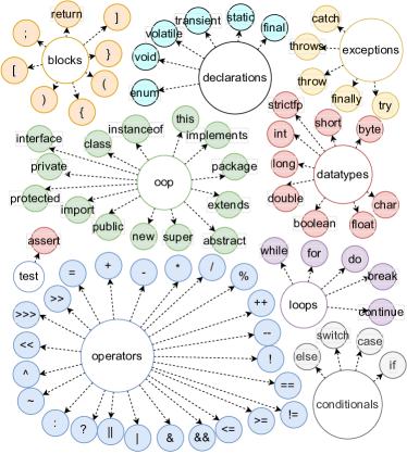
Figure 2: Structural Code Taxonomy $\mathcal{H}$ for Java

Oftentimes, it is difficult to predict whether a given NCM will be used in a similar setting to its corresponding sanitized training or testing set. To illustrate, if a model trained on a well-commented dataset is applied to predict segments of poorly commented code, this mismatch could potentially impact performance.

IV-B Component 2: Defining Structural Causal Model

In this component, assumptions about relationships among data are defined in a structural causal model similar to Fig. 1, which is later processed in the next component to compute $p(Y|do(T))$. Causal assumptions must be made explicit, which means defining the treatments $T$ (i.e., binary: buggy/non-buggy, discrete: layer modifications), potential outcomes $Y$ (i.e., global (Cross-Entropy) and local (NTPs) performance), and the common causes $Z$ that can affect the treatments and potential outcomes. For all our SCMs in this study, we assumed that common causes are SE quality metrics since they have the potential to influence models global and local performance, i.e., a NCM may be influenced by more or less for loops, as well as influence treatments, i.e., more code has been shown to be correlated with more bugs [35]. In summary, this component consists of setting down assumptions about the causal relationships of software data employed to interpret NCMs. SCMs help us to describe the relevant features of the software data and how they interact among each other. In the following subsection, we formally define our treatments and potential outcomes.

IV-B1 Defining SE Counterfactual Interventions or Treatments

NCMs are notorious for behaving differently across distinct datasets [36]. For example, if a model trained on a well-commented dataset is applied to predict segments of poorly commented code, this mismatch could potentially impact performance. As such, we assert that observing model performance across datasets with different characteristics can aid in understandability. Hence, we defined SE Counterfactual Interventions $T$ to better understand model performance across different settings. We formulate these interventions as testbeds (i.e., datasets) organized in sample pairs treatment $T=0$ (i.e., BuggyCode) and control $T=1$ (i.e., FixedCode). Note that we define testbeds according to different applications often described in SE research. The testbed preparation process is highly dependent on code properties. The general process comprises of identification of some specific intervention (i.e., program repair) and 2) construction or collection of the necessary data via mining repositories or other means that contain these interventions. More complex interventions will likely be more challenging to prepare. In do_code, counterfactual interventions produce explanations motivated by both semantic perturbations (or treatments) $T_{[data]}$ to our SE Application Settings (e.g., Buggy/Fixed, Commented/Uncommented, Clone1/Clone2) and model hyper-parameter variations $T_{[hyp]}$ on NCMs (e.g., layers, units, or heads).

IV-B2 Defining Potential Outcomes / Model Performance

Cross-Entropy (Fig. 3- ) and Next Token Prediction (Fig. 3- ) are relevant values produced at inference time that reflect the effectiveness of a model. By relating these values to counterfactual interventions $T$ (i.e., program repair), we can gain an understanding of how well a studied model is generating code under these treatments. We refer to Cross-Entropy loss as a measure of a model’s Global Performance $Y_{g}:w\to-\sum_{t\in|w|}P(w_{t}|d_{t})\log Q(w_{t}|w_{<t})$ as these losses capture the overall performance of a NCM over an entire sequence of tokens $w$. Due to the discrete nature of the data, the expression $P(w_{t}|w_{t-1:1})$ can be estimated using a classifier. The classifier, in our particular case, is a NCM [37]. Hence, rather than using n-grams or Markov Models to approximate $P(w_{t}|w_{t-1:1})$ [38], it is convenient to use a latent model $P(w_{t}|w_{t-1:1})\approx P(w_{t}|d_{t})$, where $d_{t}$ is known as a hidden state that embeds the sequence information from past observations up to the time step $t$. Depending on how the sequence is processed, the hidden state $d_{t}$ can be computed using either an autoregressive network (i.e., such as a Transformer ($TF$) [22]) or a Recurrent Neural Network ($RNN$). Conversely, Next Token Prediction (NTP) values signal Local Performance $Y_{l}:w_{<t}\to P(w_{t}|w_{t-1:1})$ within token-level contexts. NTPs capture local predictions for individual tokens that are affected by complex interactions in NCMs and are equivalent to the estimated predicted value (or softmax probability) $\sigma(k)_{t}$ for each token. Bear in mind that the size of the vector $\sigma(k)_{t}$ is the vocabulary $|\mathcal{V}|$, in which $k$ represents the non-normalized log probabilities for each output token $t$. NTPs capture the value of the expected token $w_{t}$ instead of the maximum value estimated in the vector $\sigma(k)_{t}$.

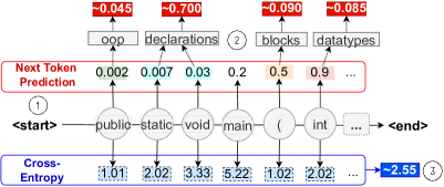
Figure 3: Potential Outcomes are Prediction Performance of NCMs: Cross-Entropy $(Y_{g})$ and Next Token Predictions $(Y_{l})$.

IV-C Component 3: Connecting SCMs with Code Corpora

According to Pearl & Mackenzie [39], CI seeks answers to questions of association (what is?), counterfactual interventions (what if?), and pure counterfactuals (why?). The authors introduce the concept of levels of causation to match distinct levels of cognitive ability with concrete actions: seeing (level 1), doing (level 2), and imagining (level 3). Our proposed analysis is primarily concerned with levels 1 & 2. Level 1 causation, namely association, $p(Y|T)$ is estimated by using typical correlation methods (e.g., Pearson, Spearman, or Covariance) in addition to functional associations such as $y=g(t)$, which can be predicted with regressions or ML methods. For binary treatments similar to the ones we used in $T_{[data]}$ (e.g., Buggy/Fixed, Commented/Uncommented, Clone1/Clone2), we opt to employ Pearson correlations and Jensen-Shannon distance as association estimand for level 1 causation. We will now formally define each of these below.

Definition 5

Jensen-Shannon Distance (JS). The Jensen-Shannon divergence (JSD) overcomes the asymmetric computation of the KL divergence and provides a measure of difference between distributions Eq. 3. The JS distance is the square of the JS divergence $p(Y|T)\approx JS(Y^{T=0},Y^{T=1})=JSD(Y^{0},Y^{1})^{2}$. JS is proportional to the influence of $T$ on $Y$, which measure the separation of the distributions $Y^{0},Y^{1}$. The notation $Y^{T=0}$ refers to the potential outcomes observed under the treatment $T=0$.

$$JSD(Y^{0}=y^{0},Y^{1}=y^{1}) =$$ (3a)

$$\frac{1}{2}\left[D_{KL}\left(y^{0}||\frac{y^{0}+y^{1}}{2}\right)+D_{KL}\left(y^{1}||\frac{y^{0}+y^{1}}{2}\right)\right] =$$ (3b)

Example 4

Imagine we wish to understand the correlation between syntactic changes, i.e., variable renaming, alterations in white space, etc. and a NCMs performance. One way we can study this is through computing the association of Cross-Entropy values $Y$ under two treatments, the first $T=0$, would be an unalterned code snippet and the second $T=1$ would be its Type III clone. Computing this association can be done using the JS distance $p(Y|T)\approx JS(Y^{0},Y^{1})$ as defined in Def. 5 for four models. Fig. 4 shows the distributions of $Y^{0}$ and $Y^{1}$ with their distances after applying bootstrapping as an example.

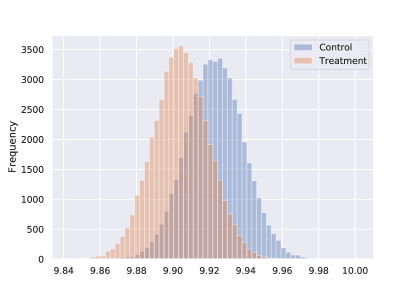
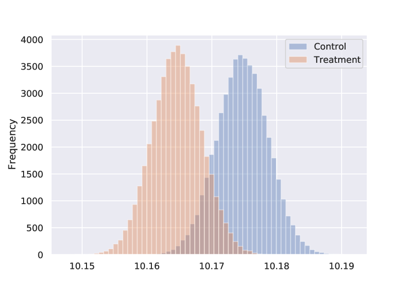
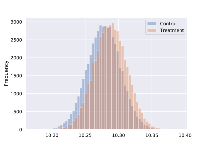
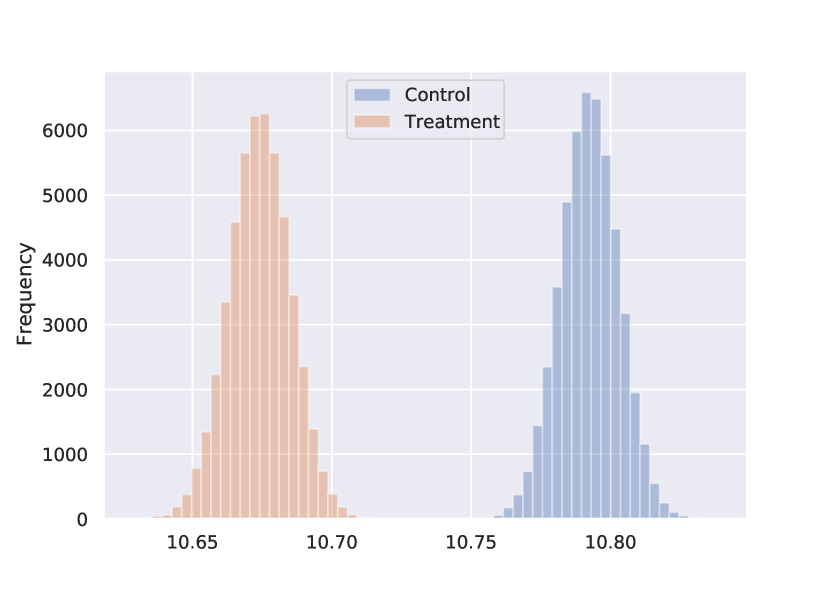
Figure 4: SemanticPreserving Intervention (BigClone3TB) for Global Performance: Bootstrapped Cross-Entropy. Top Left: RNN_1,1024 ($JS=0.3$), Top Right: GRU_1,1024 ($JS=0.8$), Bot Left: TF_6,12 ($JS=0.6$), Bot Right: TF_12,12 ($JS=1$).

Now, if we want to go beyond “what is” type questions, we must move past simple correlations and association. This requires the $do-operator$ found in level 2, causation $p(y|do(t))$. Specifically, it is estimated for a population (i.e., SE dataset) by computing an Average Treatment Effect based on the Def. 3 introduced in Sec. III.

Definition 6

Average Treatment Effect (ATE) Defining the first intervention as $do(T=1)$ and the second by $do(T=0)$, the Average Treatment Effect is the population average of the difference of causal effects of each code snippet $x$.

$$ATE=\mathbb{E}_{x\sim p(x)}[Y=y|x,do(T=t)] =$$ (4a)

$$\mathbb{E}_{x\sim p(x)}[\mathbb{E}[Y|x,do(T=1)]-\mathbb{E}[Y|x,do(T=0)]] =$$ (4b)

$$\mathbb{E}_{x\sim p(x)}[\mathbb{E}[Y^{1}|x,T=1]-\mathbb{E}[Y^{0}|x,T=0]] =$$ (4c)

IV-D Component 4: Enabling Causal Interpretability for NCMs

Average Treatment Effects (ATEs) are computed following two core steps from causal theory: identification and estimation.

IV-D1 Identifying Causal Effects

Once the SCM (similar to Fig. 1) is constructed, do_code applies various techniques (i.e., backdoor-criterion and instrumental variables) to determine the adjustment formula Eq. 2, which will control for confounding common causes when computed. For our case study, the causal effect $p(Y|do(T))$ is computed, which will be done in the next step, based on the following causal graph: data-based $T_{[data]}$ and parameter-based $T_{[hyp]}$ treatments; SE covariates $Z\in SE_{metrics}$; and potential outcomes $Y_{l},Y_{g}$.

IV-D2 Estimating Causal Effects

Next, do_code estimates the causal effect using statistical and ML methods based on the adjustment formula from the previous step. do_code computes Propensity Score Matching for binary SE treatments (i.e., Buggy/Fixed) and Linear Regressions for SE discrete treatments (e.g., layers, units, or heads). We refer interested readers to the doWhy documentation for the full process details [40]. For completeness, we will now show how to estimate a causal effect assuming a binary treatment as an example. Eq. 4 shows the formal definition of an ATE. We can derive the final expression by applying the law of total expectations and the ignorability assumption $Y\perp\!\!\!\perp Z|T$, where the potential outcomes $Y$ are independent of treatment assignments conditioned on covariates $Z$ [28]. That is, the effects of the hidden common causes $Z$ and missing data are ignored. In Eq. 4, the term $\mathbb{E}[Y^{1}|x,T=1]$ represents the expected value of a potential outcome under an observable treatment (i.e., FixedCode). Similarly, the term $\mathbb{E}[Y^{0}|x,T=0]$ represents an expected value of a potential outcome under an observable control (i.e., BuggyCode). Both terms are quantities that can be estimated from data. Covariate adjustment (in Eq. 1), propensity score (in Eq. 2c), and linear regression are some of the estimation methods that we employ to estimate the $ATE$. Their usage depends upon the type of the treatment variable (i.e., binary, discrete, or continuous) and causal graph assumptions.

IV-E Component 5: Evaluating Causal Effects

The previous causal estimation can be validated using refutation methods that calculate the robustness of the causal estimate. In essence, the refutation methods apply random perturbations to the original causal graph to test for robustness of the estimated $ATE$. We chose four methods for our analysis: Adding a random common cause or covariate $\mathcal{R}_{1}$, adding an unobserved common cause or covariate $\mathcal{R}_{2}$, replacing the treatment with a random variable or placebo $\mathcal{R}_{3}$, and removing a random subset of the data $\mathcal{R}_{4}$. For robustness, we expected that $\mathcal{R}_{1}$, $\mathcal{R}_{2}$, and $\mathcal{R}_{4}$ values were close to the $ATE$ (Eq. 4). Conversely, the placebo $\mathcal{R}_{3}$ should tend to zero.

In addition to measuring refutation methods, it is relevant to identify cases of spurious correlations (i.e., Confounding Bias) or cases where $p(Y|T)\neq p(Y|do(T))$. Typically, association is not causation due to the influence of a common cause or confounding variable $Z$. Such a variable is the one that is being controlled for or adjusted by means of Eq. 1. Nonetheless, we can still compute the correlation $d(Y|Z)$ to assess the variables that are actually affecting potential outcomes.

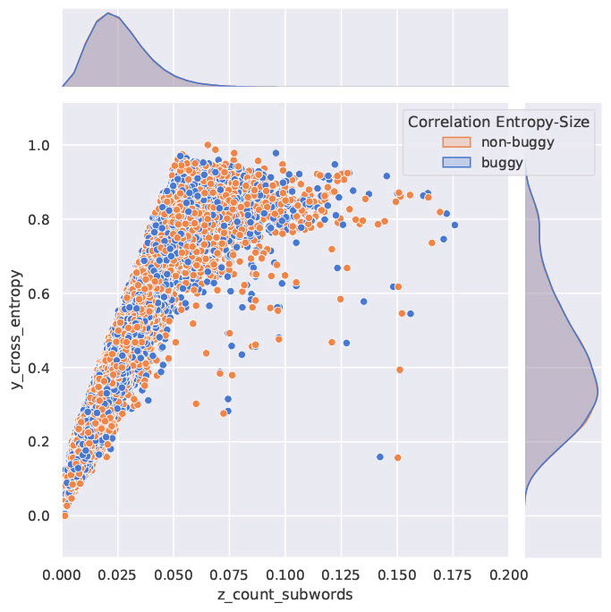
Figure 5: Spurious Correlation between the Number of Subwords common cause and Cross-Entropy values ($p(Y|Z)\approx 0.87$) for the ProgramRepair intervention generated from TF_6,12.

Example 5

Consider the ProgramRepair intervention where $T$ is Buggy/Fixed code, $Y$ is the cross-entropy of each of method of the dataset BuggyTB, and $Z$ is the Number of Subwords for each method. There exists a spurious correlation after calculating JS and ATE, $p(Y|T)\approx 0.67$ and $p(Y|do(T))\approx-0.0002$. One possible explanation is that the common cause $Z$ is confounding the relationship between the treatment and the outcome. Fig. 5 depicts the influence of $Z$ on the potential outcome $Y$ for BuggyCode ($p(Y|Z,T=Buggy)\approx 0.87$) and FixedCode ($p(Y|Z,T=Fixed)\approx 0.86$). Blue and orange points in the plot are code snippets from the dataset. These points are equally distributed, which suggest that the ProgramRepair intervention has a negligible impact on the Cross Entropy.

V Case Study Design in Code Generation

In order to illustrate the insights that do_code can enable, we present a case study that serves as a practical application of our interpretability method by analyzing two popular NCMs: RNNs and Transformers. In this section, we detail the methodological steps we took to configure our models and process our datasets. In addition, we designed our methodology for causal understanding following Pearl et al.’s guidelines [29, 41]. We adopted these guidelines to formulate two research questions: RQ₁ SE Intervention Effects and RQ₂ Stability Causation.

1. To what extent do SE data and model interventions affect code prediction performance?

   1. What is the influence of our interventions on global performance?

   2. What is the influence of our interventions on local performance?

2. How robust are the treatment effects based on SE interventions?

TABLE I: Counterfactual Interventions Case Study. NLMs include Recurrent Nets (GRUs) and Transformers (TFs).

Case Study Methodology						NCMs Training
Counterfactual Interventions				Proposed Experiments Global and Local		RNNs	Transformers	Hyper.	Val.
Type	Interv.	Case	Associated Dataset	Avg. Causation	Correlation	NCM lyr,unt	NCM lyr,hds	dropout RNN[42] dropout TF optimizer[43] learning rate beta1$|$beta2 epsilon epochs batch RNN$|$TG	0.5 0.l adam 1e-3 0.9 1e-7 64 512$|$128
Data	$T_{dat0}$	ProgramRepair	BuggyTB [31]	$p(Y_{g,l}|do(T_{dat0}))$	$p(Y_{g,l}|T_{dat0})$	RNN1,1024 GRU1,1024 GRU2,1024 GRU3,1024 GRU1,512 GRU1,2048	TF6,12 TF12,12 TF24,12
	$T_{dat1}$	UnCommenting	CommentsTB [23]	$p(Y_{g,l}|do(T_{dat1}))$	$p(Y_{g,l}|T_{dat1})$
	$T_{dat2}$	SemanticPreserving	BigClone2TB [33] BigClone3TB [33]	$p(Y_{g,l}|do(T_{dat2}))$	$p(Y_{g,l}|T_{dat2})$
Model	$T_{hyp0}$	NumberLayers	CodeSearchNet [23]	$p(Y_{g,l}|do(T_{hyp0}))$	$p(Y_{g,l}|T_{hyp0})$
	$T_{hyp1}$	NumberUnits		$p(Y_{g,l}|do(T_{hyp1}))$	$p(Y_{g,l}|T_{hyp1})$

do_code adapts causal inference theory to aid in providing explanations for both global $Y_{g}$ (RQ₁RQ_1.1) and local $Y_{l}$ (RQ₁RQ_1.2) prediction performance of given NCMs. Before do_code can be performed, a researcher or practitioner making use of our method must select the NCMs and define hyper-parameter variations $T_{[hyp]}$ and data perturbations $T_{[data]}$ that they would like to examine in Stage 1 ($St_{1}$). Here, hyper-parameter variations are essentially different configurations of a given model according to attributes such as capacity (layers) or the types of layers. Additionally, the researcher must define their code testbeds. do_code offers the possibility of adding additional testbeds with data perturbations that represent a set of SE-based interventions or Application Settings. After defining and estimating the causal effect (RQ₁) of proposed interventions in Stage 2 ($St_{2}$), do_code helps to evaluate the robustness of ATE’s results by performing refutation methods proposed in Stage 3 ($St_{3}$) (RQ₂).

V-A Context: Data Processing & Model Training

We decided to train our own subject models to have more control over the data used in training. Specifically, our choice of structural code concepts required us to have control of the tokenizer to have special tokens assigned to code concepts. However, $do_{code}$ is not limited to only working on specialized models. As long as there exists a mapping from the model level concepts (e.g., BPE tokens) to human understandable concepts (e.g., structural code concepts or ASTs as done in the code-tokenize library [44]).

To train our NCMs we made use of the Java portion of the commonly used CodeSearchNet Challenge dataset [23], which consists of a diverse set of methods (mts) from GitHub [45]. CodeSearchNet is split into a training, validation, and test set. For the testbeds for interpreting the performance of our NCMs using do_code, we collected four datasets from the CodeXGLUE project that contain control and treatment groups [46]. Tab. I shows the generated testbeds containing parallel corpora for understanding the impact of buggy code (BuggyTB: 64,722 mts), the impact of code documentation (CommentsTB: 6,664 mts), and syntactic alterations on semantically equivalent snippets based on type II (BigClone2TB: 666 mts) and type III (BigClone3TB: 8,097 mts) clones from BigCloneTB. The only additional filtering we performed on the training, validation, and testbeds was the removal of methods that contain any non-ASCII characters and, for the CommentsTB, removal of methods that do not have comments. We derived the uncommented portion of the CommentsTB by removing any existing comments from the Java test set of the CodeSearchNet dataset.

We performed Byte Pair Encoding (BPE) tokenization [47] across all testbeds before they were processed by our studied NCMs. BPE has shown to be extremely beneficial for training NCMs on code to overcome the out-of-vocabulary problem [42]. We trained a BPE tokenizer on 10% of our training data and used a vocabulary size of 10K. Due to the tokenization process of BPE, some subtokens contained multiple reserved keywords or characters if they appeared frequently together. This was problematic for our interpretability analysis since the function $\phi_{\mathcal{H}}$ relies on the ability to map model predictions to our structural taxonomy. Having certain reserved keywords and tokens merged into BPE subtokens would make it impossible for us to perform this mapping. Therefore, we fixed all reserved keywords and tokens (Fig. 2) to be detected by our trained BPE model.

As for the model training, we used Tensorflow and Pytorch [48, 49] (Huggingface’s Transformers library [50]) for creating and training our different models. Our $RNN$ and $TF$ models were trained on CodeSearchNet Java training set. All models reached optimal capacity as they all early terminated to prevent overfitting, with a patience of $5$ epochs without improvement on cross-entropy of at least $1\text{e-2}$. Additionally, we added a start of sentence token to the beginning of the input, padded and truncated all inputs to $300$. The training was executed on a 20.04 Ubuntu with an AMD EPYC 7532 32-Core CPU, A100 NVIDA GPU with 40GB VRAM, and 1TB RAM.

V-B Case Study Methodology

We provide an overview of our case study summarized in Tab. I, which follows the do_code methodology introduced in Sec. IV. This section provides the details regarding how we instantiated do_code’s methodology for our studied models and testbeds. On one hand, we empirically estimated $p(Y|T)$ using two methods: Pearson correlations and Jensen-Shannon Similarities (explained in Def. 5). On the other hand, we estimated $p(Y|do(T))$ using the doWhy library [41] and ATE (explained in Def. 6). $do_{code}$ can be used for both masked and next token prediction objectives for language models (i.e., BERT, GPT, and T5 families). While our case study only took into consideration autoregressive architectures, the definition of potential outcomes $Y$ can be easily extended to measure the performance of masked tokens.

do_code is extensible and researchers can define their own treatments. In our case study, we constructed three data interventions $T_{[data]}$ (see row Data in Tab. I). In addition, the aim of the syntax analysis was to determine how robust NCMs are in the presence of minor and major syntactic variations of semantically equivalent code snippets. That is, we assessed how semantic preserving changes affect code generation. Since there is no natural split for the different clone types, we were unable to perform a causal analysis on the BigCloneTB dataset using the typical control and treatment settings. This is because the choice of one clone compared to another is arbitrary when evaluating the set of what BigCloneTB calls function₁ and function₂ methods. Therefore, instead of our standard covariates, we used the differences between function₁ and function₂ of the different clone types. Specifically, we used the Levenshtein Distance $T_{[dat1]}$, a measure of the difference between two sequences in terms of the necessary edit operations (insert, modify, and remove) needed to convert one sequence into the other, to approximate a treatment where one method was refactored into another method by a specific number of edit operations. This formulation allowed us to avoid needing a natural split between function₁ and function₂ and focus on how syntactic differences of methods that perform the same function, i.e., semantically similar, affects our models.

As for the model interventions $T_{[hyp]}$ (see row Model in Tab. I), our case study consists of an investigation of two different NCM architectures. We also investigated how layer and unit variations in each architecture affect their performance. We made use of two different types of RNN architectures, a “base” model and a model that includes Gated Recurrent Units (GRU). Additionally, we studied a GPT-based Transformer model [51, 52] for our autoregressive model. We chose these two models because RNNs have been extremely popular in SE [53] and Transformers have recently gained popularity due to the high performance they have achieved in the NLP domain [4].

VI Results

VI-A RQ₁RQ_1.1 SE Intervention on Global Performance

TABLE II: Causal Interventions $p(Y_{g}|do(T))$ and Associations $p(Y_{g}|T)$ of Global Performance across models and datasets.

Counterfactual Interventions $T$	ProgramRepair (BuggyTB) $T_{dat0}$			UnCommenting (CommentsTB) $T_{dat1}$			NumberLayers (CodeSearchNet) $T_{hyp0}$
NCM	RNN1,1024	GRU1,1024	TF6,12	RNN1,1024	GRU1,1024	TF6,12	GRU1,1024	TF6,12
Association JS Dist./ Pearson	$0.730_{JS}$	$0.230_{JS}$	$0.670_{JS}$	$0.180_{JS}$	$0.220_{JS}$	$0.250_{JS}$	$-0.093_{PR}$	$-0.485_{PR}$
Causal Eff. ATE	-0.0003	-2.33E-05	-0.0002	0.0023	2.90E-05	0.0026	-0.0058	-0.0124
Random Comm. Cause	-0.0003	-2.45E-05	-0.0002	0.0011	-0.0004	0.0015	-0.0058	-0.0124
Unobserved Comm. Cause	-0.0003	1.54E-05	-0.0001	0.0002	-0.0001	0.0007	-0.0050	-0.0108
Placebo	0.0001	1.44E-05	0.0001	0.0006	-1.33E-05	0.0006	-0.0001	-2.77E-05
Remove Subset	-0.0003	-3.68E-05	-0.0002	0.0012	-0.0003	0.0016	-0.0058	-0.0124

TABLE III: Causal Interventions $p(Y_{g}|do(T))$ and Associations $p(Y_{g}|T)$ of Global Performance across Semantic datasets.

Counterfactual Interventions $T$	SemanticPreserving (BigClone2/3TB) $T_{dat2}$
	BigClone2TB			BigClone3TB
NCM	RNN1,1024	GRU1,1024	TF6,12	RNN1,1024	GRU1,1024	TF6,12
Association JS Dist./ Pearson	$0.45_{PR}$	$0.598_{PR}$	$0.452_{PR}$	$-0.056_{PR}$	$0.14_{PR}$	$-0.14_{PR}$
Causal Eff. ATE	0.6288	0.8713	0.5635	-0.1042	0.1085	-0.2739
Random Comm. Cause	0.6297	0.8720	0.5651	-0.1043	0.1084	-0.2741
Unobserved Comm. Cause	0.2950	0.4257	0.2737	-0.0800	0.0830	-0.2168
Placebo	-	-	-	-	-	-
Remove Subset	-	-	-	-	-	-

Tab. II and Tab. III give an overview of the different associative and interventional effects across our different models and datasets in terms of global performance. Note that the correlation row includes both Pearson and Jensen-Shannon distances. For the SemanticPreserving intervention, the association values in Tab. III indicate that Levenshtein “edit” distance between Type II clone pairs has a tendency to be positively correlated with cross-entropy values $p(Y_{g}|T_{dat2})\approx 0.60$ for GRU_1,1024. By contrast, for the Type III clones, no strong correlations were detected between syntactic and global performance differences for any of our NCMs. Nonetheless, we discovered an appreciably strong causal effect between the Levenshtein distance of clone pairs and the difference in cross-entropy with a maximum of $p(Y_{g}|do(T_{dat2}))=0.87$ for GRU_1,1024 on Type II. This suggests that our models are causally influenced by slight and major changes in syntax of programs such as white space and variable names. This is not a desired effect for code NCMs as developers have their own coding style and conventions, a NCM should perform similarly independent from the syntactic alterations.

For ProgramRepair intervention in Tab. II, it is apparent that both RNN_1,1024 and TF_6,12 exhibit considerably high JS distances. However, after controlling for SE covariates, we found that such correlations were spurious since ATEs are relatively small for the three models. The confounding is explained in Fig. 5, where the number of subwords per method is affecting the cross entropy directly beyond the ProgramRepair intervention. We have identified more confounding variables for our proposed interventions such as the Number of Unique Words, MaxNextedBlocks, and Cyclomatic Complexity. However, the variable that most influence prediction performance is the Number of Subwords per method. Similar results were found for UnCommenting (TypeIII) interventions after adjustment of covariates we saw a tendency to null causal effects. This implies that there is little to no causal influence of removing comments from the code or applying Type III syntactic changes on snippets.

As for model-based interventions, NumberLayers and NumberUnits interventions have a tendency to be negatively correlated to and to causally influence the cross-entropy. For instance, the number of units negatively affect global performance by $p(Y_{g}|T_{hpy1})\approx-0.084$ for GRU_1,1024, which is a result that aligns well with expected DL experimentation on hyperparameters. Lastly, smaller values of cross-entropy were observed once the number of layers and units increases.

VI-B RQ₁RQ_1.2 SE Intervention on Local Performance

TABLE IV: Local Association Results $p(Y_{l}|T)$ are Jensen-Shannon Dist. Causal Effects are ATEs $p(Y_{l}|do(T))$
(bold:strong corr., background:best effect)

Counterfactual Interventions $T_{data}$	ProgramRepair $T_{dat0}$						UnCommenting $T_{dat1}$
NCM	GRU1,1024			TF6,12			GRU1,1024			TF6,12
Categories	Association JS Dist.	Causal Eff. ATE	$\mathcal{R}_{1}$	Association JS Dist.	Causal Eff. ATE	$\mathcal{R}_{1}$	Association JS Dist.	Causal Eff. ATE	$\mathcal{R}_{1}$	Association JS Dist.	Causal Eff. ATE	$\mathcal{R}_{1}$
[blocks]	0.626	-0.0005	-0.00052	0.206	-0.0001	-0.000115	0.133	0.0003	0.000488	0.052	-0.0006	-0.000352
[exceptions]	0.107	-1.00E-06	1.00E-06	0.651	-1.20E-05	-1.10E-05	0.165	-4.80E-05	-4.80E-05	0.091	-1.20E-05	-4.20E-05
[oop]	0.048	2.00E-05	1.20E-05	0.058	-1.30E-05	-9.00E-06	0.070	-7.00E-06	-4.70E-05	0.090	-4.90E-05	-2.60E-05
[tests]	0.581	9.00E-06	8.00E-06	0.997	1.00E-05	9.00E-06	0.595	1.90E-05	4.00E-05	0.724	-1.70E-05	2.00E-06
[declarations]	0.071	4.00E-06	4.00E-06	0.054	1.00E-06	1.00E-06	0.061	-2.10E-05	-0.000145	0.148	4.60E-05	6.00E-05
[conditionals]	0.345	-3.90E-05	-3.90E-05	0.176	-8.00E-06	-1.00E-05	0.111	8.00E-06	7.40E-05	0.821	-0.000596	-0.000603
[loops]	0.130	-2.00E-06	-3.00E-06	0.323	2.10E-05	1.90E-05	0.027	-1.70E-05	1.50E-05	0.085	1.80E-05	3.00E-06
[operators]	0.123	-6.00E-06	-5.00E-06	0.039	1.50E-05	1.10E-05	0.278	0.0002	0.000345	0.998	0.0079	0.008991
[datatype]	0.253	-1.00E-05	-1.00E-05	0.168	9.00E-06	1.00E-05	0.749	0.0003	0.000328	0.432	0.0002	0.000111
[extraTokens]	0.169	2.60E-05	2.00E-05	0.121	5.70E-05	6.00E-05	0.368	0.0014	0.001016	0.526	0.0024	0.002004

TABLE V: Local Association Results $p(Y_{l}|T)$ are Pearson Corr. Causal Effects are ATEs $p(Y_{l}|do(T))$.

Counterfactual Interventions $T$	SemanticPreserving (Type III) $T_{dat2}$						NumberLayers $T_{hyp0}$
NCM	GRU1,1024			TF6,12			GRU1,1024			TF6,12
Categories	Association Pearson	Causal Eff. ATE	$\mathcal{R}_{1}$	Association Pearson	Causal Eff. ATE	$\mathcal{R}_{1}$	Association Pearson	Causal Eff. ATE	$\mathcal{R}_{1}$	Association Pearson	Causal Eff. ATE	$\mathcal{R}_{1}$
[blocks]	0.026	-1.50E-05	-1.50E-05	0.186	-2.80E-05	-2.80E-05	-0.102	-0.010559	-0.010559	0.725	0.018004	0.018004
[exceptions]	0.017	nan	nan	0.002	nan	nan	-0.070	nan	nan	0.349	nan	nan
[oop]	0.049	nan	nan	0.012	nan	nan	0.019	nan	nan	0.255	nan	nan
[tests]	nan	nan	nan	nan	nan	nan	-0.130	nan	nan	0.174	nan	nan
[declarations]	0.375	nan	nan	0.034	nan	nan	-0.257	nan	nan	0.405	nan	nan
[conditionals]	0.274	nan	nan	-0.087	nan	nan	-0.009	nan	nan	0.682	nan	nan
[loops]	0.024	nan	nan	0.111	nan	nan	0.042	nan	nan	0.275	nan	nan
[operators]	0.099	nan	nan	0.062	nan	nan	-0.032	nan	nan	0.389	nan	nan
[datatype]	0.037	nan	nan	-0.069	nan	nan	0.002	nan	nan	0.275	nan	nan
[extraTokens]	0.192	-3.00E-05	-3.00E-05	-0.017	5.40E-05	5.40E-05	0.092	0.014588	0.014588	0.606	0.014525	0.014525

We measured the robustness of NCMs to syntactic deviations on local performance in Tab. IV. We observed a weak causal effect between clone type variations and Next Token Predictions for all our NCMs across the 10 categories. For instance, on average, semantic Type II changes causally affected the prediction performance of object-oriented tokens $p(Y_{\texttt{\small[oop]}}|do(T_{dat2}))=0.388\pm 0.241$ and operators $p(Y_{\texttt{\small[operators]}}|do(T_{dat2}))=0.316\pm 0.202$. Semantic type III changes affected blocks of code $p(Y_{\texttt{\small[blocks]}}|do(T_{dat2}))=0.214\pm 0.107$ and declarations $p(Y_{\texttt{\small[declarations]}}|do(T_{dat2}))=0.161\pm 0.135$. Importantly, the standard deviation of these categories was quite high across the NCMs suggesting that what the models statistically learned can vary widely. We discovered that SemanticPreserving interventions affected NTP across the categories of our code taxonomy. Specifically, Levenshtein distance between Type II clones had a tendency to be positively correlated with the operators category $p(Y_{\texttt{\small[operators]}}|T_{dat2})\approx 0.56$ for GRU_1,1024. By contrast, for the Type III clones, weak correlations were perceived for Local performance (see Tab. IV). Unfortunately, most of the ATEs cannot be computed for each category because it was not possible to create a linear model to estimate the effects due to the shape of the data (i.e., input variables have the same values). As for ProgramRepair and UnCommenting interventions, $T_{dat0}$ and $T_{dat1}$ treatments had no impact on the prediction of categories in our taxonomy, as their ATEs tend to null causal effects. The maximum causal effect observed for the $do(T_{dat0})$ intervention was $p(Y_{\texttt{\small[blocks]}}|do(T_{dat0}))=-0.000525$ which corresponds with the highest correlation value for blocks category $p(Y_{\texttt{\small[blocks]}}|T_{dat0})\approx 0.6$ for GRU_1,1024, while the UnCommenting intervention was $p(Y_{\texttt{\small[operators]}}|do(T_{dat1}))=0.007949$ for TF_6,12. On the other hand, the influence of the number of layers in predicting block’s tokens in GRU_1,1024 showed a very low ATE value $p(Y_{\texttt{\small[blocks]}}|do(T_{lyr}))=-0.01$ but the highest correlation $p(Y_{\texttt{\small[blocks]}}|T_{lyr})\approx 0.7$ for TF_6,12. The other categories were unable to have their ATE calculated due to limited data. Intervening Transformer layers had only positive correlations across categories. Nonetheless, intervening layers or units in GRUs exhibited mostly negative correlations, with $p(Y_{\texttt{\small[exceptions]}}|T_{unt})=-0.25$ and $p(Y_{\texttt{\small[declarations]}}|T_{lyr})=-0.26$ for GRU_1,1024.

VI-C RQ₂ Stability of Causation

In addition to the causal effects, we also calculated four different refutation methods where applicable. For a majority of the interventions the causal effects were stable meaning our SCMs for those causal effects were accurate. The only exception to this is for the intervention $T_{dat1}$ (UnCommenting). Specifically, refutations $\mathcal{R}_{1}$, $\mathcal{R}_{2}$, and $\mathcal{R}_{4}$ should have been in the same order of magnitude as ATEs. This could be due to 1) not having enough data samples, 2) incorrect causal diagram (our assumptions of confounders, instrumental vars, and/or effect modifiers are off), and/or 3) our treatment is inadequate. Additionally, for a SemanticPreserving for refutation methods Placebo and Remove Subset we were unable to compute due to limited data. However, the other two methods, Random Comm. Cause and Unobserved Comm. Cause, were stable giving us confidence in its ATEs. This stability of our ATEs is especially important for the cases where we found a spurious correlation, i.e., $p(Y|T)\ncong p(Y|do(T))$, such as for the relatively small effect $p(Y_{g}|do(T_{lyr}))=-0.01$ of TF_6,12 that increases with the number of model layers since it originally had a relatively high correlation $p(Y_{g}|T_{lyr})\approx-0.4$.

VII Discussion

Using our approach, users are able to identify which types of code tokens were important in the model’s decision-making process. In other words, $do_{code}$ supports the identification of which 1) tokens, 2) layers, or 3) hyperparameters are impacting local or global predictions, which we describe below:

Tokens. In Sec. IV-A, we propose a mapping function (or interpretability function) for NCMs, which is able to identify how the next token prediction varies based on the types of tokens (i.e., structural code concepts). Therefore, considering this, our methodology enables determining which token types the model is able to learn (or not) across different application settings (testbeds). For example, based on our study and Fig. 6, where higher bars indicate more effective predictions across our testbeds, one could conclude that block-type tokens are important for model decision-making, given that the model seems to predict them most effectively across testbeds, whereas the models typically struggled to correctly predict operator-type tokens. More importantly, we can observe casual relationships related to how the importance of code tokens in decision-making changes across treatments (i.e., across testbeds or changes to model parameters).

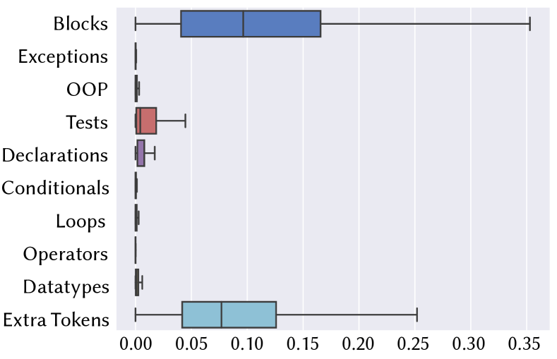
Figure 6: Code Concept Prediction Performance (Normalized CCP) for TF_6,12 on ProgramRepair (BuggyTB).

Layers. Our methodology supports interventions on the number of layers for a given architecture. Therefore, $do_{code}$ is able to identify if the layers, as a hyperparameter, are influencing the performance. Nonetheless, identifying specific layers to influence the performance would require going beyond the interpretability scope and start exploring the inner mechanisms of the neural network – a process known as explainability [20].

Hyperparemeters. $do_{code}$ supports the identification of hyperparameters that influence neural network performance by extending counterfactual intervention definitions at the model level (see Sec. IV-B). Currently, our case study supports two types of parameters: NumberOfLayers and NumberOfUnits.

Therefore, based on our experiments, NCMs seem to have a stronger “understanding” of syntax and a more limited understanding of semantics, according to our definition of semantics. In $do_{code}$, we examine model semantics by categorizing code tokens into different conceptual groups and examining both raw model performance according to these groups, and the causal relationships of these groups across treatments. Syntax can be measured by how often the model predicts a given token that is syntactically correct. While we did not directly report syntactic correctness, in our observations, our studied models rarely made syntactic errors. However, the local prediction performance of tokens across different semantic categories tended to vary quite a bit, as described in the previous response. This is partially explained by the prevalence of different token types in the training set, but further work on model architectures that improves the performance of underperforming token groups could help to advance research on NCMs.

A strong correlation across testbeds for a given code token category means that we observe the prediction performance to have changed significantly across the testbed treatments (e.g., commented/uncommented code). This change could correspond to prediction performance for these token categories increasing or decreasing. However, because our approach uses a casual graph, we can determine the amount of causal effect between the correlated variables based on covariates, and determine whether or not they are spurious (due to confounding bias Fig. 5) or true causal relationships caused by the change in treatment.

VIII Related Work

Applications of LMs in SE: LMs in SE have a rich history, stemming from the seminal work by Hindle et al. who proposed the concept of the naturalness of software using n-gram models [54]. Then, with the rise of Deep Learning, researchers began exploring the possibility of adapting NLMs to code, as initially demonstrated by White et al. [2]. Since then, LMs have been used for a number of SE tasks such as code completion [55, 56, 57, 58, 59, 38, 3, 18] and translation [6, 60, 61, 4]. Researchers have also investigated various representations of LMs for code [62] as well as graph-based representations based on ASTs [63] and program dependency graphs [64]. It has also been shown that using a LM for code representation and then fine-tuning for specific SE tasks can achieve state-of-the-art performance across tasks [65, 66, 67].

Interpretability of LMs: Many works have investigated evaluating and understanding LMs using various techniques, which can be classified into two basic groups, (i) explainability techniques such as probing for specific linguistic characteristics [68] and examining neuron activations [69]; and (ii) interpretability techniques such as benchmarks [70, 71, 23, 32, 18] and intervention analyses [72, 73, 13, 24]. Karpathy et al. were among the first to interpret NLMs for code using general Next Token Predictions [74] as an interpretability method as well as investigating individual neurons. Our work extends Karpathy et al.’s interpretability analysis using causal inference and a more statistically rigorous methodology that grounds its evaluation in SE-specific features and settings.

Complementary to our work, the work by Polyjuice paper [75] aims to automatically generate perturbations to language, to see how a given model performs in different scenarios. Our work is differentiated by the fact that we both define a mapping of source code tokens to categories, and define a methodology for linking causal relationships of model changes to these various categories. As such, our work functions alongside techniques such as Polyjuice, providing deeper insights into why model performance varies across different perturbations. Our work is also complementary to the work by Cito et al., [76] at ICSE’22 on Counterfactual explanations for models of source code. This work takes a significant step toward defining perturbations of code for counterfactual explanations of generative models. Our technique in conjunction with Cito et al.’s technique can provide deeper explanations as to why a given NCM’s performance changed for a given perturbation.

Our technique is differentiated from work on adversarial robustness via one key point, similar to the work of Cito et al. Our different testbeds are not intentionally designed to fool a model. On the contrary, our different testbeds represent completely natural distributions of code tokens collected at scale. As such, our work has a completely different aim as compared to work on adversarial robustness.

IX Adoption & Challenges of do_code

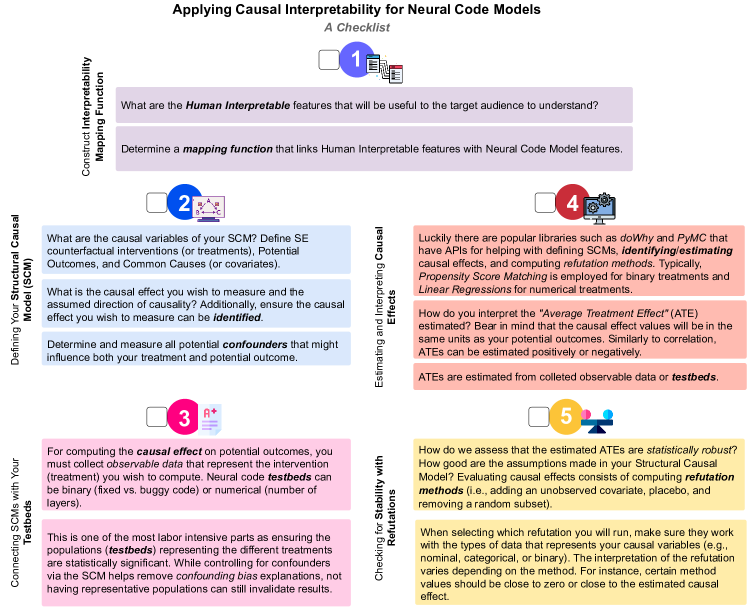
Figure 7: Guidelines for Applying Causal Interpretability to Neural Code Models.

This study leverages Pearl’s theory of Causal Inference and grounds it in interpreting Neural Code Models. One question we may have is why should we study causation in Deep Learning for Software Engineering? Causation has two main goals in science: discovering causal variables and assessing counterfactual interventions [39]. DL4SE can take advantage of the latter when dealing with uncertainty and confounding bias of NCMs. Estimating counterfactual interventions is a powerful tool to generate explanations of model’s performance. Our methodology, do_code, can be applied to a wide range of Software Researchers’ models for debugging and eliminating confounding bias. However, quantifying the effects requires the causal structure underlying the data. Randomized controlled experiments were the first option to conduct causality before Pearl’s graphical model definitions. Nonetheless, it is not practical to force developers to perform interventions like SemanticPreserving or even train hundreds of NCMs to test treatments. $do-operator$ and causal graphs are useful and better tools to perform causal estimations from observational data. Reconstructing such graphical representation is challenging since it not only requires formalizing causation in the Software Engineering field (i.e., defining potential outcomes, common causes, and treatments) but also tracing and connecting software data to causal models. In addition, formulating interventions is not an easy process. We must hypothesize feasible transformations that can occur in code to simulate real-world settings for NCMs. To that end, we have created a checklist that summarizes the general process researchers can use to apply causal interpretability to neural code models 7.

As shown in Fig. 7, there are a total of five components, which corresponds to the methodology in Sec. IV, starting with the construction of the interpretability function. In this component, a researcher determines what would be interpretable to their target audience and construct a mapping function that translates the model under study’s features to the target audience’s. Once you have this mapping, you can move on to the second component that resolves around defining a Structural Causal Model. It is important to have this step after your mapping function so that you can properly model the treatments, outcomes, and confounders. With your SCM in hand, you can now collect your data that contains the observable treatment data (e.g., buggy vs. fixed code) that will be used to estimate the causal effect of the treatment. Then, you can use existing popular libraries to estimate your causal effect. And lastly, you must check your assumptions (i.e., your confounders and SCM) using refutation methods. With this checklist, we hope to ease the complexity around causal analysis for researchers.

X Conclusion

We presented do_code, an interpretability method for understanding NCMs for code. do_code combines rigorous statistical instruments and causal inference theory to give rise to contextualized SE explanations of NCMs using Structural Causal Models (SCMs). SCMs provide a more robust and interpretable framework for modeling complex systems such as Neural Code Models in software engineering. SCMs can help to better understand the underlying mechanisms and causal relationships between different variables, which can improve the accuracy and generalizability of deep learning models. In addition, SCMs can provide a more transparent and explainable approach to Deep Learning for Software Engineering, allowing for a better understanding of the decision-making process of the model and facilitating more effective debugging and error analysis. Additionally, we also carried out a case study evaluation using do_code on popular NCMs, namely, RNNs, GRUs, and Transformers, to interpret global (i.e., cross-entropy) and local (i.e., next token predictions) performance. do_code exposes erroneous code concepts (e.g., conditionals, or loops) by examining Average Treatment Effects and refutation methods.

References

- [1] C. Watson, M. Tufano, K. Moran, G. Bavota, and D. Poshyvanyk, “On learning meaningful assert statements for unit test cases,” in Proceedings of the ACM/IEEE 42nd International Conference on Software Engineering, ser. ICSE ’20. New York, NY, USA: Association for Computing Machinery, 2020, p. 1398–1409. [Online]. Available: https://doi.org/10.1145/3377811.3380429
- [2] M. White, C. Vendome, M. Linares-Vásquez, and D. Poshyvanyk, “Toward Deep Learning Software Repositories,” in Proceedings of the 12th IEEE Working Conference on Mining Software Repositories (MSR’15), ser. MSR ’15. Piscataway, NJ, USA: IEEE Press, 2015, pp. 334–345. [Online]. Available: http://dl.acm.org/citation.cfm?id=2820518.2820559
- [3] M. Ciniselli, N. Cooper, L. Pascarella, A. Mastropaolo, E. Aghajani, D. Poshyvanyk, M. D. Penta, and G. Bavota, “An empirical study on the usage of transformer models for code completion,” 2021.
- [4] A. Mastropaolo, S. Scalabrino, N. Cooper, D. Nader Palacio, D. Poshyvanyk, R. Oliveto, and G. Bavota, “Studying the Usage of Text-To-Text Transfer Transformer to Support Code-Related Tasks,” pp. 336–347, 2021.
- [5] M. Ciniselli, N. Cooper, L. Pascarella, D. Poshyvanyk, M. D. Penta, and G. Bavota, “An empirical study on the usage of BERT models for code completion,” CoRR, vol. abs/2103.07115, 2021. [Online]. Available: https://arxiv.org/abs/2103.07115
- [6] Z. Chen, S. J. Kommrusch, M. Tufano, L.-N. Pouchet, D. Poshyvanyk, and M. Monperrus, “Sequencer: Sequence-to-sequence learning for end-to-end program repair,” IEEE Transactions on Software Engineering, pp. 1–1, 2019.
- [7] Microsoft, “Visual studio intellicode — visual studio - visual studio.” [Online]. Available: https://visualstudio.microsoft.com/services/intellicode/
- [8] “Code faster with ai code completions.” [Online]. Available: https://www.tabnine.com/
- [9] W. Zaremba, G. Brockman, and OpenAI, “Openai codex,” Aug 2021. [Online]. Available: https://openai.com/blog/openai-codex/
- [10] GitHub, “Github copilot · your ai pair programmer.” [Online]. Available: https://copilot.github.com/
- [11] G. C. Murphy, M. Kersten, and L. Findlater, “How are java software developers using the eclipse ide?” IEEE Softw., vol. 23, no. 4, p. 76–83, Jul. 2006. [Online]. Available: https://doi.org/10.1109/MS.2006.105
- [12] F. Doshi-Velez and B. Kim, “Towards A Rigorous Science of Interpretable Machine Learning,” arXiv: Machine Learning, no. Ml, pp. 1–13, 2017. [Online]. Available: http://arxiv.org/abs/1702.08608
- [13] M. T. Ribeiro, T. Wu, C. Guestrin, and S. Singh, “Beyond accuracy: Behavioral testing of NLP models with CheckList,” in Proceedings of the 58th Annual Meeting of the Association for Computational Linguistics. Online: Association for Computational Linguistics, Jul. 2020, pp. 4902–4912. [Online]. Available: https://aclanthology.org/2020.acl-main.442
- [14] R. Rei, C. Stewart, A. C. Farinha, and A. Lavie, “COMET: A neural framework for MT evaluation,” in Proceedings of the 2020 Conference on Empirical Methods in Natural Language Processing (EMNLP). Online: Association for Computational Linguistics, Nov. 2020, pp. 2685–2702. [Online]. Available: https://aclanthology.org/2020.emnlp-main.213
- [15] T. Kocmi, C. Federmann, R. Grundkiewicz, M. Junczys-Dowmunt, H. Matsushita, and A. Menezes, “To ship or not to ship: An extensive evaluation of automatic metrics for machine translation,” CoRR, vol. abs/2107.10821, 2021. [Online]. Available: https://arxiv.org/abs/2107.10821
- [16] M. Dehghani, Y. Tay, A. A. Gritsenko, Z. Zhao, N. Houlsby, F. Diaz, D. Metzler, and O. Vinyals, “The benchmark lottery,” CoRR, vol. abs/2107.07002, 2021. [Online]. Available: https://arxiv.org/abs/2107.07002
- [17] E. M. Bender, T. Gebru, A. McMillan-Major, and M. Mitchell, “On the dangers of stochastic parrots: Can language models be too big?” in Proceedings of the 2021 ACM Conference on Fairness, Accountability, and Transparency, ser. FAccT ’21. New York, NY, USA: Association for Computing Machinery, 2021, p. 610–623. [Online]. Available: https://doi-org.proxy.wm.edu/10.1145/3442188.3445922
- [18] M. Chen, J. Tworek, H. Jun, Q. Yuan, H. P. de Oliveira Pinto, J. Kaplan, H. Edwards, Y. Burda, N. Joseph, G. Brockman, A. Ray, R. Puri, G. Krueger, M. Petrov, H. Khlaaf, G. Sastry, P. Mishkin, B. Chan, S. Gray, N. Ryder, M. Pavlov, A. Power, L. Kaiser, M. Bavarian, C. Winter, P. Tillet, F. P. Such, D. Cummings, M. Plappert, F. Chantzis, E. Barnes, A. Herbert-Voss, W. H. Guss, A. Nichol, A. Paino, N. Tezak, J. Tang, I. Babuschkin, S. Balaji, S. Jain, W. Saunders, C. Hesse, A. N. Carr, J. Leike, J. Achiam, V. Misra, E. Morikawa, A. Radford, M. Knight, M. Brundage, M. Murati, K. Mayer, P. Welinder, B. McGrew, D. Amodei, S. McCandlish, I. Sutskever, and W. Zaremba, “Evaluating large language models trained on code,” 2021.
- [19] T. Wu, M. T. Ribeiro, J. Heer, and D. Weld, “Errudite: Scalable, reproducible, and testable error analysis,” in Proceedings of the 57th Annual Meeting of the Association for Computational Linguistics. Florence, Italy: Association for Computational Linguistics, Jul. 2019, pp. 747–763. [Online]. Available: https://aclanthology.org/P19-1073
- [20] C. Molnar, Interpretable Machine Learning, 2019, https://christophm.github.io/interpretable-ml-book/.
- [21] S. Hochreiter and J. Schmidhuber, “Long Short-Term Memory,” Neural Computation, vol. 9, no. 8, pp. 1735–1780, 11 1997. [Online]. Available: https://doi.org/10.1162/neco.1997.9.8.1735
- [22] A. Vaswani, N. Shazeer, N. Parmar, J. Uszkoreit, L. Jones, A. N. Gomez, Ł. Kaiser, and I. Polosukhin, “Attention is all you need,” in Proceedings of the 31st International Conference on Neural Information Processing Systems, ser. NeurIPs’17. Red Hook, NY, USA: Curran Associates Inc., 2017, p. 6000–6010.
- [23] H. Husain, H.-H. Wu, T. Gazit, M. Allamanis, and M. Brockschmidt, “CodeSearchNet challenge: Evaluating the state of semantic code search,” arXiv preprint arXiv:1909.09436, 2019.
- [24] M. R. I. Rabin, N. D. Bui, K. Wang, Y. Yu, L. Jiang, and M. A. Alipour, “On the generalizability of neural program models with respect to semantic-preserving program transformations,” Information and Software Technology, vol. 135, p. 106552, 2021.
- [25] B. Ray, V. Hellendoorn, S. Godhane, Z. Tu, A. Bacchelli, and P. Devanbu, “On the ”naturalness” of buggy code,” in Proceedings of the 38th International Conference on Software Engineering, ser. ICSE ’16. New York, NY, USA: Association for Computing Machinery, 2016, p. 428–439. [Online]. Available: https://doi.org/10.1145/2884781.2884848
- [26] Anonymous, “Interpretingcodegeneration,” https://anonymous.4open.science/r/InterpretingCodeGeneration-75E4/, 2022.
- [27] B. Schölkopf and J. von Kügelgen, “From statistical to causal learning,” 4 2022. [Online]. Available: http://arxiv.org/abs/2204.00607
- [28] J. Pearl, Causality: models, reasoning, and inference, 2009.
- [29] J. Pearl, M. Glymour, and N. P.Jewell, Causal Inference in Statistics, A Primer, 2016.
- [30] M. Allamanis, “The adverse effects of code duplication in machine learning models of code,” in Onward! OOPLSA 2019, 2019, pp. 143–153. [Online]. Available: https://doi.org/10.1145/3359591.3359735
- [31] M. Tufano, C. Watson, G. Bavota, M. Di Penta, M. White, and D. Poshyvanyk, “Learning How to Mutate Source Code from Bug-Fixes,” Proceedings - 2019 IEEE International Conference on Software Maintenance and Evolution, ICSME 2019, pp. 301–312, 2019.
- [32] S. Lu, D. Guo, S. Ren, J. Huang, A. Svyatkovskiy, A. Blanco, C. B. Clement, D. Drain, D. Jiang, D. Tang, G. Li, L. Zhou, L. Shou, L. Zhou, M. Tufano, M. Gong, M. Zhou, N. Duan, N. Sundaresan, S. K. Deng, S. Fu, and S. Liu, “Codexglue: A machine learning benchmark dataset for code understanding and generation,” CoRR, vol. abs/2102.04664, 2021.
- [33] J. Svajlenko and C. K. Roy, “Evaluating clone detection tools with BigCloneBench,” 2015 IEEE 31st International Conference on Software Maintenance and Evolution, ICSME 2015 - Proceedings, pp. 131–140, 2015.
- [34] B. Kim, M. Wattenberg, J. Gilmer, C. Cai, J. Wexler, F. Viegas, and R. Sayres, “Interpretability beyond feature attribution: Quantitative Testing with Concept Activation Vectors (TCAV),” 35th International Conference on Machine Learning, ICML 2018, vol. 6, pp. 4186–4195, 2018.
- [35] T. Menzies, J. Greenwald, and A. Frank, “Data mining static code attributes to learn defect predictors,” IEEE Transactions on Software Engineering, vol. 33, no. 1, pp. 2–13, 2007.
- [36] Y. S. Abu-Mastafa, “Learning from data.” [Online]. Available: http://work.caltech.edu/slides/slides01.pdf
- [37] Y. Bengio, R. Ducharme, and P. Vincent, “A neural probabilistic language model,” Advances in Neural Information Processing Systems, vol. 3, pp. 1137–1155, 2003.
- [38] R. M. Karampatsis, H. Babii, R. Robbes, C. Sutton, and A. Janes, “Open-Vocabulary Models for Source Code (Extended Abstract),” Proceedings - 2020 ACM/IEEE 42nd International Conference on Software Engineering: Companion, ICSE-Companion 2020, pp. 294–295, 2020.
- [39] J. Pearl and D. Mackenzie, The book of why: The New Science of Cause and Effect, 2018.
- [40] A. Sharma, E. Kiciman et al., “DoWhy: A Python package for causal inference,” https://github.com/microsoft/dowhy, 2019.
- [41] A. Sharma, V. Syrgkanis, C. Zhang, and E. Kıcıman, “DoWhy : Addressing Challenges in Expressing and Validating Causal Assumptions,” 2021.
- [42] R. M. Karampatsis, H. Babii, R. Robbes, C. Sutton, and A. Janes, “Big code != big vocabulary: Open-vocabulary models for source code,” Proceedings - International Conference on Software Engineering, pp. 1073–1085, 2020.
- [43] D. P. Kingma and J. Ba, “Adam: A method for stochastic optimization,” CoRR, vol. abs/1412.6980, 2015.
- [44] H. W. Cedric Richter, “Tssb-3m: Mining single statement bugs at massive scale,” in MSR, 2022.
- [45] github, “Github,” 2020. [Online]. Available: https://github.com/
- [46] S. Lu, D. Guo, S. Ren, J. Huang, A. Svyatkovskiy, A. Blanco, C. B. Clement, D. Drain, D. Jiang, D. Tang, G. Li, L. Zhou, L. Shou, L. Zhou, M. Tufano, M. Gong, M. Zhou, N. Duan, N. Sundaresan, S. K. Deng, S. Fu, and S. Liu, “Codexglue: A machine learning benchmark dataset for code understanding and generation,” CoRR, vol. abs/2102.04664, 2021.
- [47] R. Sennrich, B. Haddow, and A. Birch, “Neural machine translation of rare words with subword units,” arXiv preprint arXiv:1508.07909, 2015.
- [48] M. Abadi, A. Agarwal, P. Barham, E. Brevdo, Z. Chen, C. Citro, G. S. Corrado, A. Davis, J. Dean, M. Devin, S. Ghemawat, I. Goodfellow, A. Harp, G. Irving, M. Isard, Y. Jia, R. Jozefowicz, L. Kaiser, M. Kudlur, J. Levenberg, D. Mané, R. Monga, S. Moore, D. Murray, C. Olah, M. Schuster, J. Shlens, B. Steiner, I. Sutskever, K. Talwar, P. Tucker, V. Vanhoucke, V. Vasudevan, F. Viégas, O. Vinyals, P. Warden, M. Wattenberg, M. Wicke, Y. Yu, and X. Zheng, “TensorFlow: Large-scale machine learning on heterogeneous systems,” 2015, software available from tensorflow.org. [Online]. Available: https://www.tensorflow.org/
- [49] A. Paszke, S. Gross, F. Massa, A. Lerer, J. Bradbury, G. Chanan, T. Killeen, Z. Lin, N. Gimelshein, L. Antiga, A. Desmaison, A. Kopf, E. Yang, Z. DeVito, M. Raison, A. Tejani, S. Chilamkurthy, B. Steiner, L. Fang, J. Bai, and S. Chintala, “Pytorch: An imperative style, high-performance deep learning library,” in Advances in Neural Information Processing Systems 32, H. Wallach, H. Larochelle, A. Beygelzimer, F. d'Alché-Buc, E. Fox, and R. Garnett, Eds. Curran Associates, Inc., 2019, pp. 8024–8035. [Online]. Available: http://papers.neurips.cc/paper/9015-pytorch-an-imperative-style-high-performance-deep-learning-library.pdf
- [50] T. Wolf, L. Debut, V. Sanh, J. Chaumond, C. Delangue, A. Moi, P. Cistac, T. Rault, R. Louf, M. Funtowicz, J. Davison, S. Shleifer, P. von Platen, C. Ma, Y. Jernite, J. Plu, C. Xu, T. L. Scao, S. Gugger, M. Drame, Q. Lhoest, and A. M. Rush, “Transformers: State-of-the-art natural language processing,” in Proceedings of the 2020 Conference on Empirical Methods in Natural Language Processing: System Demonstrations. Online: Association for Computational Linguistics, Oct. 2020, pp. 38–45. [Online]. Available: https://www.aclweb.org/anthology/2020.emnlp-demos.6
- [51] K. Cho, B. van Merriënboer, C. Gulcehre, D. Bahdanau, F. Bougares, H. Schwenk, and Y. Bengio, “Learning phrase representations using RNN encoder–decoder for statistical machine translation,” in Proceedings of the 2014 Conference on Empirical Methods in Natural Language Processing (EMNLP). Doha, Qatar: Association for Computational Linguistics, Oct. 2014, pp. 1724–1734. [Online]. Available: https://aclanthology.org/D14-1179
- [52] A. Radford and K. Narasimhan, “Improving language understanding by generative pre-training,” 2018.
- [53] C. Watson, N. Cooper, D. Nader-Palacio, K. Moran, and D. Poshyvanyk, “A systematic literature review on the use of deep learning in software engineering research,” CoRR, vol. abs/2009.06520, 2020. [Online]. Available: https://arxiv.org/abs/2009.06520
- [54] A. Hindle, E. T. Barr, Z. Su, M. Gabel, and P. Devanbu, “On the naturalness of software,” in Proceedings of the 34th International Conference on Software Engineering, ser. ICSE ’12. IEEE Press, 2012, p. 837–847.
- [55] T. Nguyen, A. Nguyen, and H. Nguyen, “A statistical semantic language model for source code,” in ESEC/FSE 2013, 2013.
- [56] V. Raychev, M. T. Vechev, and E. Yahav, “Code completion with statistical language models,” Proceedings of the 35th ACM SIGPLAN Conference on Programming Language Design and Implementation, 2014.
- [57] Z. Tu, Z. Su, and P. Devanbu, “On the localness of software,” in Proceedings of the 22nd ACM SIGSOFT International Symposium on Foundations of Software Engineering, ser. FSE 2014. New York, NY, USA: Association for Computing Machinery, 2014, p. 269–280. [Online]. Available: https://doi-org.proxy.wm.edu/10.1145/2635868.2635875
- [58] V. J. Hellendoorn and P. Devanbu, “Are deep neural networks the best choice for modeling source code?” ESEC/FSE 2017: Proceedings of the 2017 11th Joint Meeting on Foundations of Software Engineering, pp. 763–773, 2017.
- [59] R. M. Karampatsis and C. Sutton, “Maybe deep neural networks are the best choice for modeling source code,” arXiv, no. Lm, 2019.
- [60] B. Roziere, M.-A. Lachaux, L. Chanussot, and G. Lample, “Unsupervised translation of programming languages,” in Advances in Neural Information Processing Systems, H. Larochelle, M. Ranzato, R. Hadsell, M. F. Balcan, and H. Lin, Eds., vol. 33. Curran Associates, Inc., 2020, pp. 20 601–20 611.
- [61] X. Hu, G. Li, X. Xia, D. Lo, and Z. Jin, “Deep code comment generation,” in Proceedings of the 26th Conference on Program Comprehension, ser. ICPC ’18. New York, NY, USA: Association for Computing Machinery, 2018, p. 200–210. [Online]. Available: https://doi-org.proxy.wm.edu/10.1145/3196321.3196334
- [62] M. White, M. Tufano, C. Vendome, and D. Poshyvanyk, “Deep learning code fragments for code clone detection,” in 2016 31st IEEE/ACM International Conference on Automated Software Engineering (ASE), 2016, pp. 87–98.
- [63] M. Allamanis, M. Brockschmidt, and M. Khademi, “Learning to represent programs with graphs,” in International Conference on Learning Representations, 2018. [Online]. Available: https://openreview.net/forum?id=BJOFETxR-
- [64] A. T. Nguyen and T. N. Nguyen, “Graph-based statistical language model for code,” in Proceedings of the 37th International Conference on Software Engineering - Volume 1, ser. ICSE ’15. IEEE Press, 2015, p. 858–868.
- [65] Y. Hussain, Z. Huang, Y. Zhou, and S. Wang, “Deep transfer learning for source code modeling,” Int. J. Softw. Eng. Knowl. Eng., vol. 30, pp. 649–668, 2020.
- [66] Z. Feng, D. Guo, D. Tang, N. Duan, X. Feng, M. Gong, L. Shou, B. Qin, T. Liu, D. Jiang, and M. Zhou, “CodeBERT: A pre-trained model for programming and natural languages,” in Findings of the Association for Computational Linguistics: EMNLP 2020. Online: Association for Computational Linguistics, Nov. 2020, pp. 1536–1547. [Online]. Available: https://aclanthology.org/2020.findings-emnlp.139
- [67] D. Guo, S. Ren, S. Lu, Z. Feng, D. Tang, S. LIU, L. Zhou, N. Duan, A. Svyatkovskiy, S. Fu, M. Tufano, S. K. Deng, C. Clement, D. Drain, N. Sundaresan, J. Yin, D. Jiang, and M. Zhou, “Graphcode{bert}: Pre-training code representations with data flow,” in International Conference on Learning Representations, 2021. [Online]. Available: https://openreview.net/forum?id=jLoC4ez43PZ
- [68] I. Tenney, D. Das, and E. Pavlick, “BERT rediscovers the classical NLP pipeline,” in Proceedings of the 57th Annual Meeting of the Association for Computational Linguistics. Florence, Italy: Association for Computational Linguistics, Jul. 2019, pp. 4593–4601. [Online]. Available: https://aclanthology.org/P19-1452
- [69] D. Dai, L. Dong, Y. Hao, Z. Sui, and F. Wei, “Knowledge neurons in pretrained transformers,” CoRR, vol. abs/2104.08696, 2021. [Online]. Available: https://arxiv.org/abs/2104.08696
- [70] A. Wang, A. Singh, J. Michael, F. Hill, O. Levy, and S. R. Bowman, “GLUE: A multi-task benchmark and analysis platform for natural language understanding,” in International Conference on Learning Representations, 2019. [Online]. Available: https://openreview.net/forum?id=rJ4km2R5t7
- [71] P. Rajpurkar, R. Jia, and P. Liang, “Know what you don’t know: Unanswerable questions for SQuAD,” in Proceedings of the 56th Annual Meeting of the Association for Computational Linguistics (Volume 2: Short Papers). Melbourne, Australia: Association for Computational Linguistics, Jul. 2018, pp. 784–789. [Online]. Available: https://aclanthology.org/P18-2124
- [72] U. Khandelwal, H. He, P. Qi, and D. Jurafsky, “Sharp nearby, fuzzy far away: How neural language models use context,” in Proceedings of the 56th Annual Meeting of the Association for Computational Linguistics (Volume 1: Long Papers). Melbourne, Australia: Association for Computational Linguistics, Jul. 2018, pp. 284–294. [Online]. Available: https://aclanthology.org/P18-1027
- [73] V. Prabhakaran, B. Hutchinson, and M. Mitchell, “Perturbation sensitivity analysis to detect unintended model biases,” in Proceedings of the 2019 Conference on Empirical Methods in Natural Language Processing and the 9th International Joint Conference on Natural Language Processing (EMNLP-IJCNLP). Hong Kong, China: Association for Computational Linguistics, Nov. 2019, pp. 5740–5745. [Online]. Available: https://aclanthology.org/D19-1578
- [74] A. Karpathy, J. Johnson, and F. Li, “Visualizing and understanding recurrent networks,” CoRR, vol. abs/1506.02078, 2015. [Online]. Available: http://arxiv.org/abs/1506.02078
- [75] T. Wu, M. T. Ribeiro, J. Heer, and D. Weld, “Polyjuice: Generating counterfactuals for explaining, evaluating, and improving models,” in Proceedings of the 59th Annual Meeting of the Association for Computational Linguistics and the 11th International Joint Conference on Natural Language Processing (Volume 1: Long Papers). Online: Association for Computational Linguistics, Aug. 2021, pp. 6707–6723. [Online]. Available: https://aclanthology.org/2021.acl-long.523
- [76] J. Cito, I. Dillig, V. Murali, and S. Chandra, “Counterfactual explanations for models of code,” in Proceedings of the 44th International Conference on Software Engineering: Software Engineering in Practice, ser. ICSE-SEIP ’22. New York, NY, USA: Association for Computing Machinery, 2022, p. 125–134. [Online]. Available: https://doi.org/10.1145/3510457.3513081