Sum-of-squares bounds on correlation functions in a minimal model of turbulence

Abstract

We suggest a new computer-assisted approach to the development of turbulence theory. It allows one to impose lower and upper bounds on correlation functions using sum-of-squares polynomials. We demonstrate it on the minimal cascade model of two resonantly interacting modes, when one is pumped and the other dissipates. We show how to present correlation functions of interest as part of a sum-of-squares polynomial using the stationarity of the statistics. That allows us to find how the moments of the mode amplitudes depend on the degree of non-equilibrium (analog of the Reynolds number), which reveals some properties of marginal statistical distributions. By combining scaling dependence with the results of direct numerical simulations, we obtain the probability densities of both modes in a highly intermittent inverse cascade. We also show that the relative phase between modes tends to $\pi/2$ and $-\pi/2$ in the direct and inverse cascades as the Reynolds number tends to infinity, and derive bounds on the phase variance. Our approach combines computer-aided analytical proofs with a numerical algorithm applied to high-degree polynomials.

I Introduction

Many systems in nature receive and dissipate energy on very different scales, having conservative dynamics in between, and the energy is transferred across the scales through a turbulent cascade. Among the best-known examples are isotropic fluid turbulence [1] and surface waves in the ocean [2]. The complexity of such systems makes them difficult to describe in detail, so it makes sense to consider simpler dynamical models to deepen our understanding of the statistical properties and energy transfer in such highly non-equilibrium systems [3, 4, 5].

A minimal model, which still captures the basic properties of turbulent cascades, is a system of two resonantly interacting oscillators whose natural frequencies differ by a factor of two [6]. This system allows studying direct and inverse cascades with the energy flux directed towards either higher or lower frequencies. The system has one non-dimensional governing parameter $\chi$, which plays the role of the Reynolds number. In what follows, we are mostly interested in the regime when this parameter is large, and the probability distribution tends to be singular. The analytical studies in this limit resulted in the steady-state probability density for the direct cascade, while constructing the probability density for the inverse cascade turns out to be tricky [6].

Here we apply a complementary approach to study the mode statistics in this system. We exploit the polynomial nature of dynamic equations (common for practically all turbulent systems), which allows us to impose inequalities on the correlation functions. The main idea is to find a non-negative polynomial expression, $\phi(\bm{x})-L+F(\bm{x})\geq 0$ that combines the correlation function $\phi(\bm{x})$ to be bounded, the constant value of the bound $L$, and an auxiliary polynomial function $F(\bm{x})$ that has zero mean value $\langle F(\bm{x})\rangle=0$ in a statistically steady state, which entails the inequality $\langle\phi(\bm{x})\rangle\geq L$ [7, 8]. The essence of the approach is to construct the function $F(\bm{x})$ so that the value of the lower bound $L$ is as large as possible. Although testing a polynomial expression $\phi(\bm{x})-L+F(\bm{x})$ for non-negativity is NP-hard algorithmic task, there exist numerical procedures [9, 10, 11, 12, 13] that solve the problem with a more strict requirement on the proposed expression to be sum-of-squares (SoS) of other polynomials. Moreover, these procedures allow one to maximize the value $L$ of the bound using some ansatz for the auxiliary function $F(\bm{x})$. If the ansatz is simple enough, the bound can be found analytically, while a computer algorithm can be used in advance to suggest the optimal form of the SoS polynomial. The upper bound $\langle\phi(\bm{x})\rangle\leq U$ can be constructed in a similar way. Recent examples of the application of SoS programming to study dynamical systems can be found in Refs. [7, 8, 14, 15, 16, 17].

The rest of the paper is organized as follows. In Section II, we remind the general theory behind SoS optimization and then apply the method for the two-mode system. In Section III, we present the results obtained by SoS programming for the direct cascade and compare them with the analytics and direct numerical simulations (DNS). It turns out that the upper and lower bounds for the moments of pumped and dissipating modes are close to each other and differ by less than a percent in the limit of a large Reynolds number. This allows us to determine not only their scaling dependence but also numerical values with accuracy comparable to DNS. The method can also be used to study correlations between modes, and we show that the relative phase between the modes tends to $\pi/2$ and determine upper and lower bounds for its root-mean-square fluctuations.

After the validation, in Section IV, we use the method for the inverse cascade where the probability density is unknown a priori. Analytically, we obtained only lower bounds for the correlation functions, but they demonstrate scaling consistent with the results of DNS. A numerical algorithmic analysis of the high moments of the dissipating mode leads to scaling $\langle n_{1}^{k}\rangle\propto\chi^{k-1}$, which is a fingerprint of intermittency, where $n_{1}$ is the mode intensity and $\chi$ is the Reynolds number. Based on this observation, we were able to shed light on the structure of the distribution function of this mode – the DNS results fall on the universal curve for different values of $\chi$, which has a form close to a power law with an exponential cutoff. As for the pumped mode, its statistics are close to Gaussian, and we analytically found the lower bound for its intensity $\langle n_{2}\rangle\geq 5\chi/16$ that is close to DNS. We also show that the relative phase between modes tends to $-\pi/2$ in the limit $\chi\gg 1$ and estimate the rate of this transition. Finally, we summarize and discuss our findings in Section V.

II Theoretical Framework

This section briefly explains how sum-of-squares optimization can impose inequalities on correlation functions in stochastic systems with polynomial dynamics. The presentation follows Ref. [8], where a more detailed discussion can be found.

Let us consider a stochastic dynamical system

$$\dot{x_{i}}=f_{i}(\bm{x})+\sigma_{ij}(\bm{x})\xi_{j}(t),\quad\bm{x}\in\mathbb{R}^{n},\;\bm{\xi}\in\mathbb{R}^{m},$$ (1)

where $f_{i}(\bm{x})$ and $\sigma_{ij}(\bm{x})$ are polynomial, $\xi_{i}(t)$ is a Gaussian noise with zero mean $\langle\xi_{i}(t)\rangle=0$ and the variance $\langle\xi_{i}(t)\xi_{j}(t^{\prime})\rangle=\delta_{ij}\delta(t-t^{\prime})$, and here and below we sum over repeated indices. We assume that the system has reached a statistical steady-state, and then the probability density function $\rho(\bm{x})$ satisfies the stationary Fokker-Planck equation

$$\frac{1}{2}\partial_{i}[\sigma_{ij}\partial_{k}(\sigma_{kj}\rho)]-\partial_{i}(f_{i}\rho)=0.$$ (2)

We also assume that the solution to this equation is unknown. We wish to prove a constant lower bound $\langle\phi(\bm{x})\rangle\geq L$ for some polynomial correlation function $\phi(\bm{x})$, where the angle brackets mean the averaging over the probability density $\rho(\bm{x})$.

For this purpose, we consider an auxiliary function $Q(\bm{x})$, which does not grow fast when $|\bm{x}|\to\infty$, so that all the moments considered below are finite. Performing integration by parts and neglecting boundary terms, one can show that $\langle\frac{1}{2}\sigma_{kj}\partial_{k}(\sigma_{ij}\partial_{i}Q)+f_{i}\partial_{i}Q\rangle=0$. The idea is to properly design $Q(\bm{x})$ so that

$$\left\langle\frac{1}{2}\sigma_{kj}\partial_{k}(\sigma_{ij}\partial_{i}Q)+f_{i}\partial_{i}Q+\phi-L\right\rangle\geq 0\ .$$ (3)

Evaluation of the expectation in expression (3) requires knowing $\rho(\bm{x})$, but it is sufficient for the inequality to hold point-wise for all $\bm{x}$.

Checking a polynomial expression for non-negativity is NP-hard algorithmic task, therefore to reduce computational complexity, it can be replaced with a semidefinite programming (SDP) problem of checking the stronger condition that expression (3) belongs to a set of polynomials that are sum-of-squares (SoS). Finally, to find the maximum value of the constant $L$, we arrive at the following optimization problem

$$\max_{Q(\bm{x})}L:\;\frac{1}{2}\sigma_{kj}\partial_{k}(\sigma_{ij}\partial_{i}Q)+f_{i}\partial_{i}Q+\phi-L\in SoS.$$ (4)

One specifies an ansatz for the auxiliary function $Q(\bm{x})$ with undetermined coefficients and then solves the problem using the software packages such as SOSTOOLS [11], YALMIP [12] or SumOfSquares.jl [13] with one of the appropriate SDP-solvers [18, 19, 20, 21]. The upper bounds $\langle\phi(\bm{x})\rangle\leq U$ can be obtained in a similar way by considering the optimization problem

$$\min_{Q(\bm{x})}U:\;-\frac{1}{2}\sigma_{kj}\partial_{k}(\sigma_{ij}\partial_{i}Q)-f_{i}\partial_{i}Q-\phi+U\in SoS.$$ (5)

If the ansatz is simple enough, the bounds $L$ and $U$ can be found analytically, and the computer algorithm suggests the optimal form of the SoS polynomials. The more complex ansatz leads to more rigorous bounds; however, complex ansatz requires more computational efforts, and the numerical algorithm could fail to find an optimal solution.

III Direct cascade

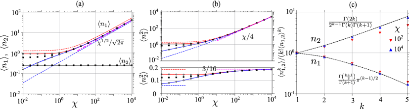
Figure 1: Average values of mode intensities (a), their second (b), and higher moments (c) for the direct cascade. Solid and dashed lines show numerical ($d=10$) and analytical ($d=4$) results for the upper (red) and lower (blue) bounds. The square markers present results of DNS, and dash-dotted lines correspond to asymptotics following from relation (8). Expressions for the asymptotic dependence are shown in the panels.

The direct cascade for the two-mode system is governed by the following non-dimensional system of equations [6]

$$\displaystyle\dot{b}_{1}=-\frac{2ib_{1}^{*}b_{2}}{\sqrt{\chi}}+\xi(t),$$ (6)

$$\displaystyle\dot{b}_{2}=-\frac{ib_{1}^{2}}{{\sqrt{\chi}}}-b_{2},$$ (7)

where $b_{1}$ and $b_{2}$ are complex envelopes of low- and high-frequency modes, respectively, $\xi(t)$ is a complex Gaussian random force with zero mean $\langle\xi(t)\rangle=0$ and the variance $\langle\xi(t)\xi^{*}(t^{\prime})\rangle=\delta(t-t^{\prime})$, and the asterisk means complex conjugate. In other words, real and imaginary parts of $\xi(t)$ are independent white noises having zero mean values and intensities $1/2$. The parameter $\chi$ is the only control parameter in the system, and it quantifies the dissipation relative to interaction strength. In the statistical steady-state, the energy input rate equals the energy flux from the first mode to the second and the dissipation rate. For the amplitude of the dissipating mode and the flux, one finds $\langle n_{2}\rangle\equiv\langle|b_{2}|^{2}\rangle=1/4$, $\langle J\rangle\equiv\langle ib_{1}^{2}b_{2}^{*}+c.c.\rangle/\sqrt{\chi}=-1/2$.

In the limit $\chi\ll 1$, the interaction between modes is strong, and the energy transfer is fast, so one may expect that the occupation numbers are close to energy equipartition $\langle|b_{1}|^{2}\rangle\equiv\langle n_{1}\rangle=2\langle n_{2}\rangle$ corresponding to thermal equilibrium [6]. The DNS shows that the marginal distributions of the mode amplitudes are indeed close to the Gaussian statistics with the corresponding occupation numbers. Still, the phase between the modes $\theta=\arg(b_{1}^{2}b_{2}^{*})$ is unevenly distributed, which indicates the presence of correlations between the modes [6].

In the opposite limit of weak interaction and strong noise, $\chi\gg 1$, one expects that the driven mode needs much higher amplitude to provide for the flux: $\langle n_{1}\rangle\gg\langle n_{2}\rangle$. In other words, the mode statistics are far from thermal equipartition. In this case, the asymptotic analytical solution for the whole distribution function was argued to be singular [6]:

$$\mathcal{P}(b_{1},b_{2})=\frac{2^{3/2}}{\pi^{3/2}\chi^{1/2}}\exp\left(-\frac{2}{\chi}|b_{1}|^{4}\right)\delta\left(b_{2}+\frac{ib_{1}^{2}}{\sqrt{\chi}}\right)\ .$$ (8)

We will use this result later for comparison with the results of our approach, which provides mutual validation.

Let us now apply the SoS optimization method described in the previous section. To proceed, we need to specify an ansatz for the auxiliary function $Q$. We have found that the numerical procedure works better if $Q$ is a polynomial with respect to $n_{1},\ n_{2},\ J$ and takes the monomials $n_{1}^{i}n_{2}^{j}J^{k}$ with the total degree of mode amplitudes less than $d\geq 2i+2j+3k$. A more general ansatz does not improve estimates for the correlation functions, but the algorithm is less stable due to the expansion of the optimization space. Let us emphasize that for small values of $d$, the bounds for the correlation functions can be obtained analytically, the computer algorithm operates for higher values of $d$ and improves the result.

We begin to present our results with the intensity of the pumped mode. For $d=4$ we obtain analytically [22]

$$\frac{\chi^{1/2}}{2\sqrt{2}}\leq\langle n_{1}\rangle\leq\dfrac{1}{2}\left(3-\sqrt{3}+\sqrt{12-6\sqrt{3}+\chi}\right),$$ (9)

and in the limit $\chi\gg 1$, this implies ${\chi^{1/2}}/{2\sqrt{2}}\leq\langle n_{1}\rangle\leq\sqrt{\chi}/2$. Inequality (9) means, in particular, that the intensity of the pumped mode is much greater than the intensity of the dissipated mode, and $\langle n_{1}\rangle/\langle n_{2}\rangle\propto\sqrt{\chi}$. As the parameter $d$ increases, the numerically found upper and lower bounds for $d=10$ approach very closely the asymptotic $\langle n_{1}\rangle=\sqrt{\chi/2\pi}$ following from expression (8), see Fig. 1a. In the opposite case $\chi\ll 1$, the upper bound $\langle n_{1}\rangle\leq 3-\sqrt{3}$ does not depend on $\chi$ in qualitative agreement with DNS. The lower bound is not tight, and increasing the parameter $d$ does not qualitatively change its behavior.

Similar results are also obtained for higher moments of $n_{1}$. For the second moment and $d=4$ we analytically find [22]

$$\chi^{2}r_{l}(\chi)\leq\langle n_{1}^{2}\rangle\leq\frac{\chi}{4}+\chi^{2}r_{u}(\chi),$$ (10)

where $r_{l}(\chi)$ is the largest real root of the equation $1-\chi^{2}r+8\chi^{3}r^{2}-16\chi^{4}r^{3}=0$ and $r_{u}(\chi)$ is the smallest positive real root of the equation $1+16\chi+(4\chi+152\chi^{2})r+(348\chi^{3}-32\chi^{4})r^{2}-216\chi^{5}r^{3}+16\chi^{7}r^{4}=0$. In the limit $\chi\gg 1$, the upper and lower bounds coincide with each other and therefore $\langle n_{1}^{2}\rangle\to\chi/4$, while in the opposite case $\chi\ll 1$, one obtains $2^{-4/3}\chi^{2/3}\leq\langle n_{1}^{2}\rangle\lesssim 1.88$, where the upper bound reflects scaling consistent with DNS, see Fig. 1b. For even higher moments of $n_{1}$, the values in the limit $\chi\gg 1$ can be determined numerically with good accuracy since the upper and lower bounds tend to each other as $d$ increases. Analyzing the values of the moments, one can conclude that the statistics of the mode $b_{1}$ are essentially non-Gaussian in agreement with expression (8), see Fig. 1c. This kind of analysis can help one to guess the marginal distribution function if it is not known a priori.

Next, we turn to the dissipating mode. Its mean intensity is determined exactly from the energy balance condition, $\langle n_{2}\rangle=1/4$, and the upper and lower bounds for $\langle n_{2}^{2}\rangle$ are shown in Fig. 1b. In the limit $\chi\gg 1$, the reasonable bounds are obtained for relatively large values of $d\geq 6$, so we do not present analytical results. In the opposite case $\chi\ll 1$, the bounds demonstrate scaling consistent with DNS, but they are not close to each other. Analytically we obtain $1/16\leq\langle n_{2}^{2}\rangle\leq 3/16$ for $d=4$ and $\chi\ll 1$ [22]. The analysis of higher moments for $\chi\gg 1$ is presented in Fig. 1c, and the results are in agreement with the marginal distribution $P(b_{2})=\frac{2^{1/2}}{\pi^{3/2}|b_{2}|}e^{-2|b_{2}|^{2}}$ following from expression (8).

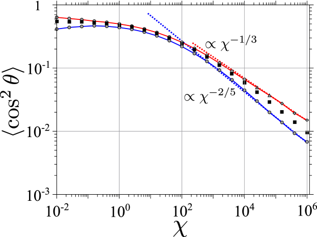
Figure 2: Relative phase between modes for the direct cascade: numerically obtained upper (red) and lower (blue) bounds (circles, triangles, and diamonds are for $d=10,\ 12,\ 14)$; the square markers present results of DNS.

The SoS programming method can also be used to analyze correlations between modes. To estimate the relative phase between modes, we rewrite the initial equations (6)-(7) in terms of real variables $\rho_{1}=|b_{1}|$, $\rho_{2}=|b_{2}|$, $\theta=\arg(b_{1}^{2}b_{2}^{*})$:

$$\dot{\rho_{1}}=-\dfrac{2\rho_{1}\rho_{2}\sin\theta}{\sqrt{\chi}}+\dfrac{1}{4\rho_{1}}+\dfrac{\zeta_{1}(t)}{\sqrt{2}},$$ (11)

$$\dot{\rho_{2}}=\dfrac{\rho_{1}^{2}\sin\theta}{\sqrt{\chi}}-\rho_{2},$$ (12)

$$\dot{\theta}=\dfrac{\rho_{1}^{2}-4\rho_{2}^{2}}{\rho_{2}\sqrt{\chi}}\cos\theta+\dfrac{\sqrt{2}\zeta_{2}(t)}{\rho_{1}},$$ (13)

where the overall phase drops out, and $\zeta_{i}(t)$ is a real Gaussian noise with zero mean and the pair correlation function $\langle\zeta_{i}(t)\zeta_{j}(t^{\prime})\rangle=\delta_{ij}\delta(t-t^{\prime})$ [22]. Despite the right-hand sides of these equations are not polynomial, for any functions $Q$ and $\phi$ that are polynomial with respect to $\rho_{1}$, $\rho_{2}$, $\sin\theta$ the expressions in left-hand sides of Eqs. (4), (5) are polynomials divided by $\rho_{1}^{2}\rho_{2}>0$. Thus, to apply the algorithm, it is sufficient to multiply the expression in the optimization problems (4), (5) by $\rho_{1}^{2}\rho_{2}>0$ to return it into the class of polynomial functions, see details in Ref. [22]. Now the ansatz for the function $Q$ is a polynomial of $\rho_{1},\ \rho_{2},\ \sin\theta$ of the power of $d$. We have also found that the numerical procedure gives better results if we solve the optimization problem with the additional constraint $1-\sin^{2}\theta\geq 0$ [22].

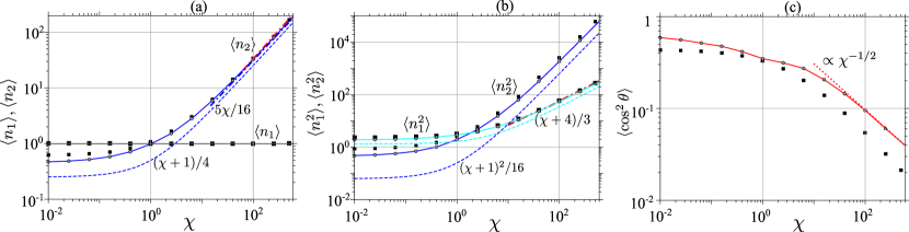
Figure 3: Average values of mode intensities (a), their second moments (b), and the relative phase (c) for the inverse cascade. Solid and dashed lines show numerical ($d=10$) and analytical results for upper and lower bounds. The square markers present results of DNS, and dash-dotted lines correspond to asymptotic bounds in the limit $\chi\gg 1$. Expressions for the analytic results are shown in the panels.

Fig. 2 shows the upper and lower bounds on $\langle\cos^{2}\theta\rangle$. The value of $\langle\cos^{2}\theta\rangle\to 0$ as $\chi\to\infty$, which means that the phase $\theta\to\pi/2$ (the point $\theta=-\pi/2$ is not suitable because $\langle J\rangle\equiv\langle-2\rho_{1}^{2}\rho_{2}\sin\theta\rangle/\sqrt{\chi}=-1/2<0$). The power-law fit $\langle\cos^{2}\theta\rangle\propto\chi^{-q}$ results in $q=1/3$ and $q=2/5$ for the upper and lower bounds, respectively. We could not determine the bounds analytically since the algorithm gives reasonable estimates only for large values of $d$. The overall picture is that the distribution function of the phase between the modes has a peak at $\theta=\pi/2$, and its width decreases in a power-law manner with the parameter $\chi$. These results complement Ref. [6], in which the narrowing of the phase distribution was not quantified.

IV Inverse cascade

Now we turn to the inverse cascade where the high-frequency mode is pumped, and the low-frequency mode dissipates

$$\displaystyle\dot{b}_{1}=-\frac{2ib_{1}^{*}b_{2}}{\sqrt{\chi}}-b_{1},$$ (14)

$$\displaystyle\dot{b}_{2}=-\frac{ib_{1}^{2}}{{\sqrt{\chi}}}+\xi(t).$$ (15)

In the statistical steady-state, from the energy balance consideration, we find $\langle n_{1}\rangle\equiv\langle|b_{1}|^{2}\rangle=1$ and $\langle J\rangle\equiv\langle ib_{1}^{2}b_{2}^{*}+c.c.\rangle/\sqrt{\chi}=1$, which is true for any value of $\chi$. The energy flux $\langle J\rangle$ is positive that corresponds to the transfer of energy down the frequencies. As in the case of a direct cascade, in the limit $\chi\ll 1$, one can expect the occupation numbers to be close to the energy equipartition $\langle n_{1}\rangle=2\langle n_{2}\rangle$, although the statistics is not expected to be close to the product of two Gaussians corresponding to thermal equilibrium. In the opposite case $\chi\gg 1$, the system is far from thermal equilibrium, and the pumped mode is expected to have larger intensity, $\langle n_{2}\rangle\gg\langle n_{1}\rangle$. All these expectations were confirmed by DNS [6].

We found that we can get better bounds for correlation functions if we rewrite dynamic equations (14)-(15) in terms of real variables $\rho_{1}=|b_{1}|$, $\rho_{2}=|b_{2}|$, $\theta=\arg(b_{1}^{2}b_{2}^{*})$:

$$\dot{\rho_{1}}=-\dfrac{2\rho_{1}\rho_{2}\sin\theta}{\sqrt{\chi}}-\rho_{1},$$ (16)

$$\dot{\rho_{2}}=\dfrac{\rho_{1}^{2}\sin\theta}{\sqrt{\chi}}+\dfrac{1}{4\rho_{2}}+\dfrac{\zeta_{1}(t)}{\sqrt{2}},$$ (17)

$$\dot{\theta}=\dfrac{\rho_{1}^{2}-4\rho_{2}^{2}}{\rho_{2}\sqrt{\chi}}\cos\theta+\dfrac{\zeta_{2}(t)}{\sqrt{2}\rho_{2}},$$ (18)

where the overall phase drops out [22]. We also found that in contrast to the direct cascade, it is useful to extend the ansatz for the function $Q$ by adding the term $\log\rho_{1}$. The term $\log\rho_{2}$ does not have a noticeable effect on the results. The left-hand sides of Eqs. (4), (5) should be multiplied by $\rho_{2}^{2}>0$ so that they become polynomial and we can apply the SDP algorithm to solve the optimization problem [22].

In contrast to the direct cascade, we were able to obtain only lower bounds for the correlation functions in the case of the inverse cascade. The algorithm does not find a feasible solution for the upper bounds, even for a relatively large parameter value $d=10$. Fortunately, the lower bounds are quite informative precisely in the turbulent limit of large $\chi$ which we focus on. In particular, for the intensity of the pumped mode, we analytically find [22]

$$\langle n_{2}\rangle\geq\dfrac{\chi+1}{4},$$ (19)

and both asymptotics at $\chi\ll 1$ and $\chi\gg 1$ give a scaling that agrees qualitatively with DNS, see Fig. 3a. Physically, inequality (19) means that in the limit $\chi\gg 1$, the intensity of the pumped mode is much greater than the intensity of the dissipating mode, $\langle n_{2}\rangle/\langle n_{1}\rangle\geq\chi/4$. We thus have shown that deviation from the equipartition is much stronger in the inverse cascade than in the direct one (where the ratio is $\propto\sqrt{\chi}$).

Similarly, we find for the amplitude fourth moment [22]

$$\langle n_{2}^{2}\rangle\geq\dfrac{(\chi+1)^{2}}{16},\quad\langle n_{1}^{2}\rangle\geq\dfrac{\chi+4}{3}.$$ (20)

The first condition is trivial and follows from the positive variance of the pumped mode intensity. The second condition means that in the limit $\chi\gg 1$, the ratio $\langle n_{1}^{2}\rangle/\langle n_{1}\rangle^{2}\geq\chi/3$, i.e., the statistics of the dissipated mode is intermittent. This agrees with the analysis carried out in Ref. [6], where it was shown that the $\rho_{1}$ dynamics is a sequence of burst events, see also Fig. 4a. Between bursts, the amplitude $\rho_{1}$ is close to zero, and during short bursts with a duration of order unity, $\rho_{1}$ reaches large values $\sim\sqrt{\chi}$. The time interval between bursts is $\sim\chi$, and the correlation functions of $\rho_{1}$ saturate on bursts. In Fig. 3b, we compare the obtained inequalities with DNS. All asymptotics demonstrate correct scaling with the parameter $\chi$. Note that analytical inequalities are improved by the numerical algorithm when we increase the parameter $d$.

Fig. 3c shows the upper bound for $\langle\cos^{2}\theta\rangle\leq U$,which is equivalent to the lower bound for $\langle\sin^{2}\theta\rangle\geq 1-U$. In the limit $\chi\gg 1$, the value of $\langle\cos^{2}\theta\rangle\to 0$ and it means that the the phase $\theta\to-\pi/2$, since the value of $\langle J\rangle=\langle-2\rho_{1}^{2}\rho_{2}\sin\theta\rangle/\sqrt{\chi}=1$. The power-law fit $\langle\cos^{2}\theta\rangle\propto\chi^{-q}$ results in $q=1/2$, although the interval is short and with increasing $\chi$ we have to increase $d$ so that the algorithm finds a feasible solution. Compared to the direct cascade, the phase fluctuations in the inverse cascade are smaller for the same value of $\chi$. Based on this observation, we can simplify equations (16)-(18) by assuming that the relative phase is locked on $\theta=-\pi/2$. Then, we obtain

$$\dot{\rho_{1}}=\dfrac{2\rho_{1}\rho_{2}}{\sqrt{\chi}}-\rho_{1},$$ (21)

$$\dot{\rho_{2}}=-\dfrac{\rho_{1}^{2}}{\sqrt{\chi}}+\dfrac{1}{4\rho_{2}}+\dfrac{\zeta(t)}{\sqrt{2}},$$ (22)

and these equations can be used to improve the above bounds in the limit $\chi\gg 1$. In particular, for the intensity of the pumped mode, we analytically obtain $\langle n_{2}\rangle\geq 5\chi/16$ [22], which is closer to DNS results, see Fig. 3a.

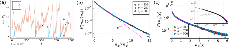
Figure 4: (a) DNS fragment of the mode dynamics for the inverse cascade demonstrate intermittency of the dissipated mode, $\log_{10}\chi=2.4$; (b) Probability density for the pumped mode in the inverse cascade. The dashed line corresponds to the exponential distribution, $P(x)=e^{-x}$; (c) Reduced probability density $F(n_{1}/\chi)$ for the dissipating mode in the inverse cascade, see Eq. (23). The inset shows the same data in the log-log scale, and the dashed line corresponds to the numerical fit $F(x)=1.7x^{-1}e^{-1.7x}$. The bin size is $0.05$ for the main panel and $0.001$ for the inset.

The reduction in the number of degrees of freedom allows us to use larger values of parameter $d$ in the limit $\chi\gg 1$ since the size of the optimization space is also reduced. Moreover, we were able to obtain upper bounds ($d=32$) for correlation functions $\langle n_{2}\rangle$ and $\langle n_{1}^{2}\rangle$, which are close to the lower bounds, see Figs. 3a and 3b. To estimate the higher moments of both modes, we will further use the values of lower bounds obtained for $d=32$. In this way, for the pumped mode, we found the usual scaling $\langle n_{2}^{k}\rangle\propto\langle n_{2}\rangle^{k}$ [22]. In the intervals between bursts, the amplitude $\rho_{1}$ is close to zero, and, according to Eq. (15), one can expect that the statistics of the pumped mode is close to Gaussian. The value $\langle n_{2}\rangle$ can be estimated as a diffusion displacement during the time between bursts, $\langle n_{2}\rangle\sim\chi$, in agreement with the results reported earlier. The DNS data for the probability density function confirm this qualitative analysis, although the agreement is not perfect, see Fig. 4b.

For the dissipating mode, we found that $\langle n_{1}^{k}\rangle\propto\chi^{k-1}$ [22], and such scaling is a fingerprint of intermittence discussed above. This suggests that in the limit $\chi\gg 1$, the distribution function of the dissipating mode has the following form:

$$P(n_{1}/\chi)=\dfrac{1}{\chi}F(n_{1}/\chi).$$ (23)

DNS confirms this hypothesis and Fig. 4c shows the reduced probability density function $F(x)$, which is proportional to $1/x$ for $x\ll 1$ and has an exponential cutoff for $x\gtrsim 1$.

A simplified model for the dynamics of the dissipating mode explains the exponent $-1$ of the power law and resolves the singularity at $x\to 0$. During the burst, the amplitude $\rho_{2}$ of the pumped mode quickly diminishes (see Fig. 4a), therefore the second term in Eq. (14) dominates and the subsequent dynamics of the dissipating mode corresponds to the exponential decay, $\dot{x}=-2x$. For a given $x$, the probability density is determined by the time spent in the vicinity of $x$ and thus proportional to $F(x)\propto 1/|\dot{x}|\propto 1/x$. The exponential dynamics is valid until the amplitude of the pumped mode is below $\sim\sqrt{\chi}$. In this regime, the pumped mode grows due to diffusion and reaches the level of $\sqrt{\chi}$ in time of the order of $\chi$, so the dependence $F(x)\propto 1/x$ holds for $x\gtrsim e^{-2\chi}$. This value should be taken as the lower limit of integration in the expression for the total probability to resolve the singularity. Since the minimum value of $x$ depends on the parameter $\chi$, the height of the first bin on the histograms is proportional to $\chi$. Except for this, the shape of the curve $F(n_{1}/\chi)$ is universal, see Fig. 4c.

When calculating the positive moments of $x$, the singularity disappears and the lower limit of integration can be replaced by zero. From the condition $\langle n_{1}\rangle=1$ we obtain $\int_{0}^{\infty}xF(x)dx=1$, and so the function has the form $F(x)\simeq ax^{-1}e^{-ax}$. Numerical fitting leads to $a\approx 1.7$, and the corresponding curve is shown in Fig. 4c by a dashed line.

V Conclusion

So what have we learned about the statistics of the far from the equilibrium state of the system using SoS programming? We obtained computer-aided analytical and numerical bounds for correlation functions in the system of two interacting modes in the regimes corresponding to both direct and inverse energy cascades. The bounds revealed the scaling of mode intensities and their higher moments with the Reynolds number $\chi$, which shows how far the system is from the energy equipartition corresponding to the thermal equilibrium. By combining scaling dependence with DNS, we collapsed the probability densities of dissipating and pumped modes on the universal curves in a highly intermittent regime of the inverse energy cascade and determined their shapes. Analyzing cross-mode correlations, we showed that the relative phase between modes tends to $\pi/2$ and $-\pi/2$ in the direct and inverse energy cascades, respectively, and estimated the rates of these transitions.

The method applied does not work well in the opposite limit of low Reynolds number $\chi\ll 1$. This can be explained by the fact that the term produced by the white noise forcing in the optimization problems (4) has a relatively small amplitude and, therefore, the expression that is analyzed practically coincides with the case of a deterministic problem, which has a trivial solution $b_{1}=b_{2}=0$, and for this reason the lower bound does not exist. Methods for overcoming this issue are discussed in Ref. [8], but we did not use them since the regime $\chi\ll 1$ is less interesting for us from the physical point of view.

Let us also note that the direct and inverse cascades are very different, although the equations at first glance may seem similar. In the direct cascade, the dissipating mode is excited by the pumped mode in an additive way. For the inverse cascade, this process is multiplicative, and the general experience suggests that this regime is more complicated because of higher temporal intermittency. Our analysis supports this intuition: in the inverse cascade we were able to obtain only lower bounds for the correlation functions, while for the direct cascade, we obtained both lower and upper bounds, and they are so close that we can determine the numerical values of the correlation functions with an accuracy comparable to DNS.

It would be promising to extend the present study to other shell models of turbulence with longer chains of resonantly interacting modes [5, 23]. The main difficulty is that for the long chains the extreme modes in the correlation function of interest will be coupled to the modes adjacent to them, and therefore the dynamic equations for the subset of modes involved in the correlation function are not closed. A similar problem arose when applying the sum-of-squares method to the Galerkin expansion of the Navier-Stokes equation in Ref. [7]. Although the generalization is not straightforward, the development of a complementary approach for this analysis significantly advances this area of research.