Tracking the spectral properties across the different epochs in ESO 511-G030

The Type I active galactic nucleus (AGN) ESO 511-G030, a formerly bright and soft-excess dominated source, has been observed in 2019 in the context of a multi-wavelength monitoring campaign. However, in these novel exposures, the source was found in a $\displaystyle\sim$10 times lower flux state, without any trace of the soft-excess. Interestingly, the X-ray weakening corresponds to a comparable fading of the UV suggesting a strong link between these components. The UV/X-ray spectral energy distribution (SED) of ESO 511-G030 shows remarkable variability. We tested both phenomenological and physically motivated models on the data finding that the overall emission spectrum of ESO 511-G030 in this extremely low flux state is the superposition of a power-law-like continuum ($\displaystyle\Gamma\sim$1.7) and two reflection components emerging from hot and cold matter. has Both the primary continuum and relativistic reflection are produced in the inner regions. The prominent variability of ESO 511-G030 and the lack of a soft-excess can be explained by the dramatic change in the observed accretion rate, which dropped from an L/L_Edd of 2% in 2007 to 0.2% in 2019. The X-ray photon index also became harder during the low flux 2019 observations, perhaps as a result of a photon starved X-ray corona.

1 Introduction

The broadband emission in active galactic nuclei (AGNs) can be ascribed as an interplay between thermal and non-thermal processes taking place in the close surroundings of a central supermassive black hole (SMBH; see Padovani et al., 2017, for an overview on AGNs). Accretion onto the SMBH is responsible for the optical-UV emission and a fraction of these thermal photons is intercepted and Comptonised up to the X-rays by the so-called hot corona (e.g. Galeev et al., 1979; Haardt & Maraschi, 1991, 1993). Our knowledge on this plasma is still lacking, though timing and microlensing arguments (e.g. Chartas et al., 2009; Morgan et al., 2012; De Marco et al., 2013; Kara et al., 2016) support the hypothesis of this component being compact and located in the inner regions of the accretion flow.
The presence of this hot plasma well explains the cut-off power-law like continuum of AGNs with the high energy roll over being interpreted as a further signature of the inverse-Compton of seed photons by the thermal plasma of electrons with E_c depending on the temperature of the relativistic electrons (kT) (Rybicki & Lightman, 1979). The characterisation of the primary X-ray continuum has been the focus of several studies (e.g. Perola et al., 2000; Dadina, 2007; Molina et al., 2009, 2013; Malizia et al., 2014; Ricci et al., 2018) and it has been boosted after the launch of NuSTAR Harrison et al. (2013a) as demonstrated by the increasing number of high energy cut-off measurements (e.g. Baloković et al., 2020; Reeves et al., 2021; Kamraj et al., 2022).
Reflection off Compton-thin/thick matter imprints additional features to the emerging X-ray spectrum. This is the case of the fluorescence Fe K$\displaystyle\alpha$ emission line at 6.4 keV (e.g. Bianchi et al., 2009) or the Compton-hump (George & Fabian, 1991; Matt et al., 1993; García et al., 2014). Noticeably, the analysis of the Fe K$\displaystyle\alpha$ profile carries a wealth of information on the location of the reflecting materials. In fact, its intrinsically narrow profile, can undergo distortions, resulting into a broader shape, due to relativistic effects (e.g. Fabian et al., 1989; Tanaka et al., 1995; Fabian et al., 2000; Nandra et al., 2007; de La Calle Pérez et al., 2010).
Finally the soft X-ray band of AGNs ubiquitously show a bump of counts below $\displaystyle\sim$2 keV that is not accounted by the high energy power-law continuum (e.g Piconcelli et al., 2005; Bianchi et al., 2009; Gliozzi & Williams, 2020). The origin of this component, the so-called soft-excess, is still debated and two possible scenarios have been tested on various data-sets: blurred ionised reflection and warm Comptonisation (e.g. Crummy et al., 2006; Magdziarz et al., 1998; Jin et al., 2012; Done et al., 2012). Both these models have been found to reproduce the data: Walton et al. (2013) tested the relativistic reflection origin of the soft-excess on a broad number of Seyfert galaxies using Suzaku data (see also Crummy et al., 2006), while the so-called two-coronae model was found to best-fit the broadband emission spectrum of an increasing number of AGNs (e.g. Petrucci et al., 2018; Porquet et al., 2018; Kubota & Done, 2018; Ursini et al., 2018, 2020; Mahmoud & Done, 2020; Matzeu et al., 2020; Middei et al., 2020).
Variability is another key feature of AGNs emission (Bregman, 1990; Mushotzky et al., 1993; Wagner & Witzel, 1995; Ulrich et al., 1997). Spectral variations are characterised by a softer-when-brighter behaviour that is commonly observed in nearby Seyfert galaxies and unobscured quasars (e.g. Sobolewska & Papadakis, 2009; Serafinelli et al., 2017, respectively). X-ray amplitude variations have been witnessed over different time-intervals, from hourly (Ponti et al., 2012) up to yearly changes (Vagnetti et al., 2016; Paolillo et al., 2017; Middei et al., 2017; Falocco et al., 2017; Gallo et al., 2018; Timlin et al., 2020). X-ray variability has been found to anti-correlate with the source luminosity, with this being naturally explained if changes result by the superposition of $\displaystyle N$ randomly emitting sub-units. This scenario, already considered in optical studies (e.g. Pica & Smith, 1983; Aretxaga et al., 1997), predicts a variability amplitude $\displaystyle\propto N^{-0.5}\propto L^{-0.5}$ and accounts for the sub-units to be identical and flare independently (e.g. Green et al., 1993; Almaini et al., 2000). Interestingly, this behaviour has been reported by many authors, both for local and high-redshift AGNs also in the X-rays (e.g. Barr & Mushotzky, 1986; Lawrence & Papadakis, 1993; Papadakis et al., 2008; Vagnetti et al., 2011, 2016).
In this context, we report on the X-ray spectral properties of ESO 511-G030, a nearby ($\displaystyle z=0.02239\pm 0.00001$, Theureau et al., 1998) spiral galaxy (de Vaucouleurs et al., 1991) hosting an unobscured type 1 AGN (Véron-Cetty & Véron, 2010). One of the first X-ray spectra of ESO 511-G030 was taken with ASCA in 1998 (Turner et al., 2001b) in which the source spectrum was best-fitted using an absorbed power-law, while a subsequent INTEGRAL-based analyses allowed to measure a high energy cut-off E_c=100${}^{+101}_{-37}$ keV (Malizia et al., 2014). The AGN ESO 511-G030 is reported in the 105-month BAT catalog (Oh et al., 2018), with a flux of $\displaystyle\sim$4$\displaystyle\times$10^-11 erg s^-1 cm^-2 (14-195 keV) and is one of the 13 objects in the FERO sample, an XMM-Newton-based collection of AGNs with a ¿5$\displaystyle\sigma$ detection of a relativistic iron line (details in de La Calle Pérez et al., 2010). In a recent paper by Ghosh & Laha (2020), who studied a 2007 XMM-Newton exposure, the source flux was consistent with F${}_{2-10\leavevmode\nobreak\ keV}\sim$2$\displaystyle\times$ 10^-11 erg s^-1 cm^-2. In the same paper, two Suzaku observations, five years apart from the XMM-Newton one, are also discussed. In those observations, the source flux was compatible with the XMM-Newton 2007 observation and, in the second one, about 50% higher. Moreover, ESO 511-G030 do not show the presence of cold and/or warm absorption components (e.g. Laha et al., 2014), leaving the soft X-ray band free from complex absorption features, and only a modest attenuation of the UV emission.
The paper is organised as follows: Sect. 2 reports on data reduction and in Sect. 3 the timing properties of the observations are discussed. In Sect. 4 we describe the spectral analyses of the XMM-Newton/NuSTAR 2019 monitoring campaign where we test the same spectral model on the archival data in Sect. 5. Then Sect. 6 and Sect. 7 describe the broadband Swift data analysis including XRT and UVOT data. In Sect. 8 we tested a self-consistent model on the 2019 and the 2007 XMM-Newton exposures also considering optical monitor (OM) data. Our conclusions and comments are reported in final Sect. 9.

2 Data reduction

Table 1: Log of the observations. The $\displaystyle\dagger$ identify exposures from the joint XMM-Newton-NuSTAR monitoring campaign

Observatory	Obs. ID	Start date	Net exp.
		yyyy-mm-dd	ks
ASCA	76067000	1998-02-06	17
XMM-Newton	0502090201	2007-08-05	120
Suzaku	707023010	2012-07-20	5.7
Suzaku	707023020	2012-07-22	224
Suzaku	707023030	2012-08-17	51
XMM-Newton$\displaystyle\dagger$	0852010101	2019-07-20	35
NuSTAR	60502035002	2019-07-20	52
XMM-Newton$\displaystyle\dagger$	0852010201	2019-07-25	37
NuSTAR	60502035004	2019-07-25	49
XMM-Newton$\displaystyle\dagger$	0852010301	2019-07-29	35
NuSTAR	60502035006	2019-07-29	51
XMM-Newton$\displaystyle\dagger$	0852010401	2019-08-02	40
NuSTAR	60502035008	2019-08-02	48
XMM-Newton$\displaystyle\dagger$	0852010501	2019-08-09	35
NuSTAR	60502035010	2019-08-09	51

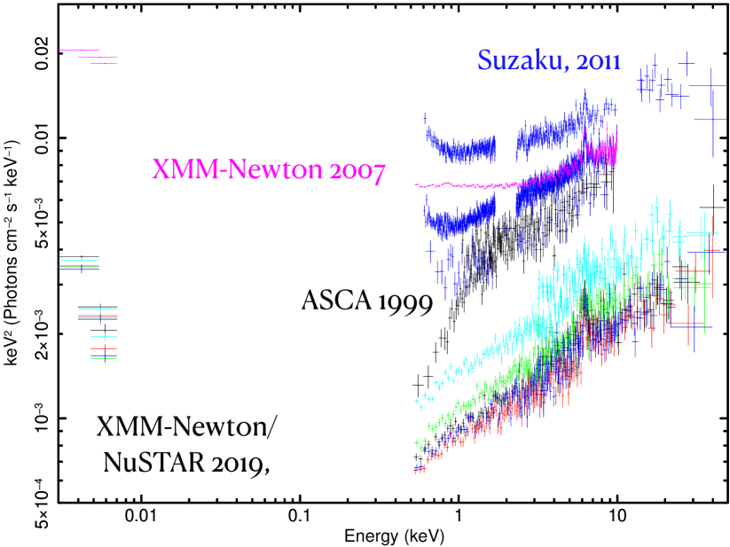
Figure 1: Unfolded spectra of ESO 511-G030 corresponding to the observations quoted in Table 1. Variability is observed both in terms of spectral and amplitude changes. In the optical/UV band the source faded by a factor of $\displaystyle\sim$10. The underlying model folding the data is a power-law with $\displaystyle\Gamma$=2 and a unitary normalisation.

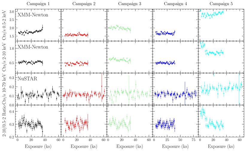
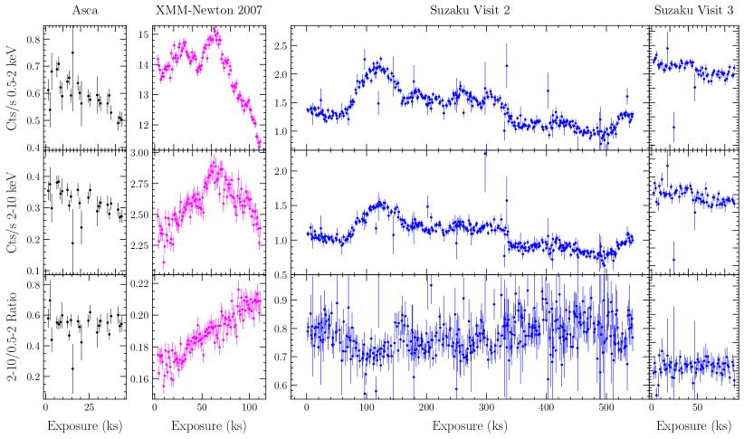
Figure 2: Top panels: Background subtracted light curves from the 2019 multiwavelength campaign. The first two rows refer to the XMM-Newton 0.5-2 and 2-10 keV, respectively, while the last one shows the ratios between these two bands. Finally, NuSTAR light curves extracted in the 10-79 keV band are showed. Bottom panels: background subtracted time series for ASCA (black), the 2007 XMM-Newton orbit (red) and the Suzaku visits 2 and 3 (in blue).

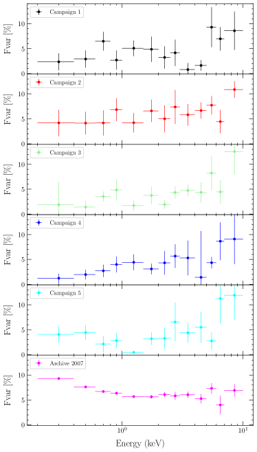
Figure 3: F_var spectra for the XMM-Newton observations in Table 1. Spectra from the 2019 monitoring campaign are all characterised by a fairly flat shape while data from 2007 clearly show a variability bump in the soft X-rays.

We present the analysis of our multi-wavelength XMM-Newton/NuSTAR observational campaign from 2019 and we compare it with data taken using different facilities across a time interval longer than 20 years. In Table 1 the log of the observations is reported while in Fig. 1 we show a quick look of all spectra simply folded with a power-law ($\displaystyle\Gamma$=2), from which it is possible to witness the remarkable variations of ESO 511-G030 in both the X-ray and optical/UV bands.

• ASCA: We retrieved the already reduced data products of ESO 511-G030 from the Tartarus ASCA AGN database (Turner et al., 2001b)
  

• Suzaku: ESO 511-G030 was observed with Suzaku (Mitsuda et al., 2007) on July 20th (OBSID: 707023010), 22th (707023020) and August 6th (707023030) 2012 through the X-ray Imaging Spectrometer (XIS; Koyama et al., 2007) for net exposure times of $\displaystyle 5.7\,\rm ks$, $\displaystyle 224\,\rm ks$ and $\displaystyle 51\,\rm ks$ respectively. Following the processes described in the Suzaku data reduction guide, the XIS 0, 1 and 3 CCD spectra were extracted with HEASOFT (v6.29.1) and adopting the latest version of the CALDB (November 2021). The cleaned event files were selected from the 3$\displaystyle\times$3 and 5$\displaystyle\times$5 edit modes and subsequently processed according to the suggested screening criteria. Both XIS source and background spectra were extracted from circular regions of radius $\displaystyle 3.0$ arcmin. Care was also taken in avoiding the chip corners containing the Fe⁵⁵ calibration sources. The corresponding spectra and lightcurves were subsequently extracted using xselect for the second and third observations as the first pointing is too short. For each detector, the response matrices (RMF) and the ancillary response files (ARF) were generated by running the xisrmfgen and xissimarfgen tasks. After verifying their consistency, we combined the front illuminated (XIS-FI) 0 and 3 spectra into a single XIS03-FI spectrum for observations 707023020 and 707023030. We used a cross-calibration constant to account for the inter-calibration between the XIS and Pin detectors. In the fits, this constant has its expected value k$\displaystyle\sim$1.16 for the 707023030 data only while it goes to a value of k$\displaystyle\sim$1.50 in the 707023020 observation. Such a particularly high value for this constant is explained by the non-simultaneity of the XIS-PIN exposures due to telemetry issues which occurred leaded to an actual shortening of the PIN exposure to about 1/5 of what was scheduled. Then, the high value of the cross-correlation constant is straightforwardly explained by the intra-observation variability that the source had undergone.
  

• XMM-Newton: We reduced and analysed both a 120 ks 2007 XMM-Newton orbit and the five exposures about 30 ksec each that were obtained simultaneously with NuSTAR in 2019. The exposures were performed with the EPIC camera (Strüder et al., 2001; Turner et al., 2001a) operating in the Small Window mode. Data were processed using the XMM-Newton Science Analysis System (SAS, Version 19.0.0). Because of its larger effective area with respect to the MOS cameras, we only report the results for the pn instrument. Source spectra were derived using a circular region with a 40 arcsec radius centered on the source while the background was extracted from a blank 50 arcsec radius area nearby the source. The extraction regions were selected using an iterative process that maximises the S/N similarly to what described in Piconcelli et al. (2004). The spectra were rebinned in order to have at least 30 counts for each bin and not to over-sample the spectral resolution by a factor greater than 3. Finally, from the epatplot, pile-up issues are not affecting this dataset.

• NuSTAR: We calibrate and clean raw NuSTAR (Harrison et al., 2013b) data using the NuSTAR Data Analysis Software (NuSTARDAS, Perri et al., 2013) package (v. 1.8.0). Level 2 cleaned products were obtained with the standard nupipeline task while 3rd level science products were computed with the nuproducts pipeline and using the calibration database 20191219. A circular region with a radius of 50 arcsec was used to extract the source spectrum. The background has been calculated using the same circular region but centered in a blank area nearby the source. To account for the inter-calibration of the two modules carried on the NuSTAR focal plane, we used in all the fits a cross-normalisation constant. Such a calibration constant was always found to be within 3% this indicating the FPMA/B spectra to be in good agreement. Spectra were binned so that each bin has at least 50 counts and to not over-sample the instrumental resolution by a factor greater than 2.5.
  

• Swift: the satellite observed ES0511-G030 from 2018 to 2021 and we reduced data acquired with XRT and UVOT. The X-ray telescope XRT observed the source in photon counting mode and we derived the corresponding scientific products using the facilities provided by the Space Science Data Center, (SSDC,https://www.ssdc.asi.it/) of the Italian Space Agency (ASI). In particular, spectra were extracted adopting a circular region of $\displaystyle\sim$60 arcsec centered on the source and a concentric annulus was used for the background. Then spectra have been binned in order to have at least 5 counts in each bin. The UVOT aperture photometry was used then to obtain the monochromatic fluxes for all the available filters. A source extraction region of 5 arcsec radius was adopted and an appropriate blank annular region concentric with the source was adopted for the background.
  

All the errors quoted in Tables and text account for 90% uncertainties, while 68% errors are shown in the plots. Fits are performed using Xspec (Arnaud, 1996) assuming the standard cosmological framework given by H₀ = 70 Km s^-1 Mpc^-1, $\displaystyle\Omega_{\Lambda}$=0.73, and $\displaystyle\Omega$m=0.27.

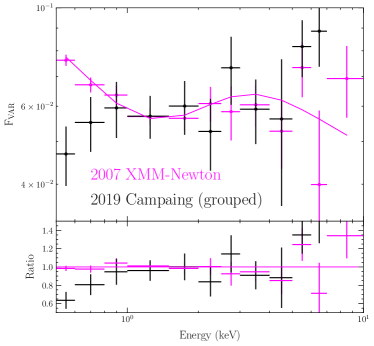
Figure 4: Comparison between the F_var spectrum of the 2007 (magenta) and 2019 (black) observations respectively, where the latter was obtained by grouping together the 5 observations via the standard command setplotgroup within XSPEC. The magenta curve represents a theoretical F_var spectrum which accounts for combined contribution from a variable power-law-like continuum and a variable soft-excess.

3 Timing properties

We extracted the background subtracted light curves for all the observations. In the top panels of Fig. 2 we show the soft and hard X-ray light curves of the 2019 monitoring campaign time series while those of archival observations ( XMM-Newton and Suzaku) are shown in the bottom panels. From Fig.2, both short- and long- term variability characterises the ESO 511-G030 light curves. During 2019, ESO 511-G030 had a quite stable behaviour with both the soft and hard X-rays being fairly constant within each exposure and among the different pointings. Such a constancy, apart from a small fraction of the fifth exposure, can be observed in the ratios panels. This constant behaviour suggests that the balance between soft and hard X-rays did not change during the campaign. The flat shape of the 2019 hardness ratios can be quantitatively(qualitatively) compared with those computed from XMM-Newton(Suzaku) archival exposures. The ratios between the 0.5-2 and 2-10 keV bands was more variable in the 2007 XMM-Newton exposure with changes of about 25%. Hardness ratios from Suzaku show moderate variations within the same exposure and varied of $\displaystyle\sim$10% on daily rather than monthly timescales.
Short-term X-ray variations are related to the intrinsic properties of the AGN such as its SMBH mass or its luminosity (e.g. Vaughan et al., 2003; Papadakis, 2004; McHardy et al., 2006). Ponti et al. (2012) computed the normalised excess variance of ESO 511-G030 using the 2007 XMM-Newton light curves. Such a variability estimator allowed the authors to derive the black hole mass of ESO 511-G030 to be $\displaystyle\log$M_BH=7.89${}_{-0.20}^{+0.30}$ M_☉.
Another commonly adopted estimator suitable for X-ray variability characterisation is the fractional root mean square variability amplitude (F_var, e.g. Edelson et al., 2002; Vaughan et al., 2003; Ponti et al., 2004). The F_var tool is the square root of the normalised excess variance and it has been widely used to characterise the variability properties of AGN in X-rays (e.g. Vaughan et al., 2004; Ponti et al., 2006; Matzeu et al., 2016, 2017; Alston et al., 2019; Parker et al., 2020; De Marco et al., 2020; Igo et al., 2020; Middei et al., 2020). We studied the variability properties of ESO 511-G030 by computing the F_var spectra for each of the 2019 XMM-Newton observations. These spectra sample variability on timescales ranging between $\displaystyle\sim 1-40$ ks. We used the background subtracted light curves extracted in different energy intervals and adopting a temporal bin of 1000 sec. Following the same procedure, we also computed the F_var spectrum of the 2007 XMM-Newton observation. The latter, samples longer timescales ranging between $\displaystyle\sim 1-120$ ks, and enables us to identify variable spectral components contributing to the time-averaged spectrum. The resulting F_var spectra of each observation are shown in Fig. 3. The errors are computed using Eq. B2 of Vaughan et al. (2003) and account only for the uncertainty caused by Poisson noise.
Aside from some excess towards the high energy region of the spectra (e.g., due to residual background variability), all the observations from the 2019 monitoring show a rather flat F_var spectrum, therefore implying a similar variability power across different energy bands. On the contrary, the 2007 F_var spectrum clearly shows a divergence, from the 2019, in the soft X-rays, consistent with the presence of an additional variability component.
To better highlight this, in Fig. 4 we overlay the 2007 F_var spectrum and the grouped F_var spectra from the 2019 campaign. We used publicly available table models to describe the 2007 F_var spectrum in terms of combined contribution from flux variability of a power-law-like continuum and a soft-excess. While the model well reproduces the 2007 F_var spectrum and the high energy part of the 2019 data, it clearly overestimates the soft band part of the 2019 F_var spectrum. One possible explanation is the presence of an additional soft variability component in 2007 which is not present in the 2019 data.

4 Spectral properties: the XMM-Newton/NuSTAR 2019 campaign

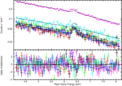
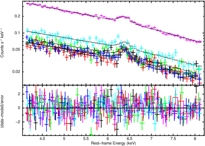
Figure 5: Top panels: EPIC-pn data in the 4-8 keV energy band fitted using a power law and a narrow Gaussian emission line assumed to be constant among the exposures. Residuals in the Fe K energy range are present. Bottom panels: Same as above but with the addition of a broad Fe K$\displaystyle\alpha$ emission line for which the line normalisation was assumed to be constant among the 2019 pointings but free to vary in 2007.

4.1 The Fe K$\displaystyle\alpha$ complex

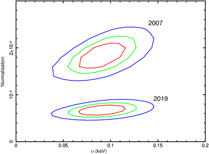
Figure 6: Confidence regions at 99%, 90% and 68% for the line’s width and normalisation. These contours have been obtained assuming the model power-law+zGauss_broad. Contours were obtained using a single broad Gaussian component.

We begun our investigation by focusing on 2019 EPIC-pn spectra (between 4 and 8 keV) and the properties of the Fe K$\displaystyle\alpha$ emission line. We adopted two components, a power-law and Gaussian line assumed to be narrow ($\displaystyle\sigma$=0 eV) and centered at 6.4 keV. We simultaneously fitted all the spectra computing the photon index (we assumed its value to be the same among the pointings) and the power-law normalisation. For the Gaussian component, we calculated its normalisation in all the exposures. This simple fit returned a Fe K$\displaystyle\alpha$ flux consistent with being constant, Norm_FeKα= (6.8$\displaystyle\pm$0.8)$\displaystyle\times$10^-6 photons cm^-2 s^-1. We then considered the 2007 XMM-Newton data on the 4-8 keV energy range on which we tested the same model and further assumed the Fe K$\displaystyle\alpha$ to have the same normalisation between 2007 and 2019. In other words, we only fitted the photon index and the normalisation of the continuum for this newly added data, see top panel Fig. 5. However, the narrow emission line only reproduces the 2019 spectra and an additional broader component is required for the 2007 data. We thus froze the narrow Gaussian component to its best-fit value and added a new broad Gaussian emission line. In the fit, the line energy centroid and width were computed and we assumed these values to be the same among the all observations. We only allowed the line’s normalisation to vary between the 2019 dataset and the 2007 exposure. This new model resulted in the fit of Fig. 5, bottom panel, with $\displaystyle\chi^{2}$/d.o.f.=400/310. We subsequently re-fit the data also allowing the narrow Gaussian normalisation to vary between the datasets. This test resulted in a slight benefit in terms of statistic with $\displaystyle\Delta\chi^{2}$/$\displaystyle\Delta$d.o.f.=-10/-1. However, in this case, only an upper limit is returned for the narrow Gaussian components’ flux.
We further tested the origin of the Fe K$\displaystyle\alpha$ emission line computing the fit once again but only including a broad Gaussian component. Again we assumed the line’s energy centroid and width to be the same across the years and only its normalisation was calculated separately for the 2019 and 2007 data. Interestingly, this step led to a statistically equivalent fit $\displaystyle\chi^{2}$/d.o.f.=400/310, which suggests the Fe K$\displaystyle\alpha$ in ESO 511-G030 to be consistent either with a superposition of a narrow and constant core plus a broad and variable component or with a single and moderately broad Gaussian that varies in time becoming stronger at a higher continuum flux. This is illustrated in Fig. 6, whereby the line normalisation for a single broadened Gaussian significantly decreased between the high flux 2007 and low flux 2019 observations. This behaviour, quite at odds with what commonly observed in AGNs, was also seen in NGC 2992 Marinucci et al. (2020).

4.2 Spectral modelling

We investigated the broadband spectral properties of ESO 511-G030 by testing a purely phenomenological model. We modelled the XMM-Newton/NuSTAR data with a cut-off power-law absorbed for the Galaxy (N_H= 4.33$\displaystyle\times 10^{20}$ cm^-2, HI4PI Collaboration et al., 2016), a moderately broad Gaussian component for the Fe K$\displaystyle\alpha$, and a thermal component to account for curvature in the soft band (Model A). We fitted separately each observation and we report the inferred best-fit values and the statistic associated to each fit in Table 2. This procedure revealed that no significant spectral variations occurred during the campaign. The Fe K$\displaystyle\alpha$ was constant in terms of normalisation and in all but observations 2 and 4 the line profile was consistent with being broad. The high energy cut-off was constrained in observations 1 and 5 while only lower limits were obtained in the remaining exposures. At lower energies, a weak and constant black-boky-like component did not vary among the different observations. Given the little variability among the parameters, we fitted simultaneously all the observations tying the photon index, the cut-off energy for the primary continuum, the energy centroid and width of the Gaussian component and the temperature and normalisation of the black body. This resulted into a fit with $\displaystyle\chi^{2}$=1470 for 1416 d.o.f and an associated null probability of 0.1. Moreover we found a $\displaystyle\Gamma$=1.62$\displaystyle\pm$0.02 while the high energy roll over was as E_c¿160 keV. For the Fe K$\displaystyle\alpha$ we obtained E_FeKα=6.39$\displaystyle\pm$0.02, $\displaystyle\sigma_{\rm FeK\alpha}$=70$\displaystyle\pm 30$ and a normalisation of Norm_FeKα=7.2$\displaystyle\pm 1.8\times 10^{-6}$ photons cm^-2 s^-1, in full agreement with the results reported in Sect 4.1.

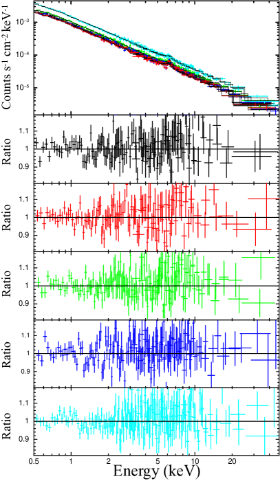
Figure 7: Model C fitting the to the 2019 spectra. Borus and relxill account for the cold and hot reflection components, respectively.

Table 2: Best-fit parameters obtained using models A and B (see Sect. 4.2 for details). The corresponding statistics are also showed. For the sake of simplicity, we only quote the constant accounting for the XMM-Newton spectra as those for FPMA&B are always within a 10% it. Finally, the L39 quantity refers to the luminosity in units of 10³⁹ erg s^-1 and D₁₀ is the distance in units of 10 kpc, as defined in the XSPEC manual (see, https://heasarc.gsfc.nasa.gov/xanadu/xspec/manual/node137.html.

Model	Comp.	Par.	Obs. 1	Obs. 2	Obs. 3	Obs. 4	Obs. 5	Units
Model A
	blackbody	kT	0.15$\displaystyle\pm$0.02	0.15$\displaystyle\pm$0.01	0.15$\displaystyle\pm$0.02	0.15$\displaystyle\pm$0.02	0.14$\displaystyle\pm$0.01	eV
		Norm	6.0$\displaystyle\pm$0.8	5.2$\displaystyle\pm$0.8	5.8$\displaystyle\pm$0.7	4.8$\displaystyle\pm$1.1	9.5$\displaystyle\pm$1.2	$\displaystyle\times 10^{-6}$ L39
	cut-off pl	$\displaystyle\Gamma$	1.64$\displaystyle\pm$0.02	1.64$\displaystyle\pm$0.02	1.63$\displaystyle\pm$0.03	1.65$\displaystyle\pm$0.01	1.61$\displaystyle\pm$0.01
		Ecut	160${}^{+175}_{-75}$	¿100	¿345	¿100	150${}^{+100}_{-50}$	keV
		Norm	9.4$\displaystyle\pm$0.1	8.4$\displaystyle\pm$0.1	10.8$\displaystyle\pm$0.1	9.0$\displaystyle\pm$0.2	15.5$\displaystyle\pm$0.2	$\displaystyle\times 10^{-4}$ ph keV-1 cm-2 s-1
	zGauss	E	6.42$\displaystyle\pm$0.09	6.38$\displaystyle\pm$0.03	6.39$\displaystyle\pm$0.12	6.40$\displaystyle\pm$0.04	6.38$\displaystyle\pm$0.10	keV
		$\displaystyle\sigma$	100${}^{+140}_{-90}$	¡65	290$\displaystyle\pm$75	¡120	170${}^{+200}_{-100}$	eV
		Norm	7.6$\displaystyle\pm$2.2	8.6$\displaystyle\pm 1.3$	8.8$\displaystyle\pm$2.0	8.3$\displaystyle\pm$	9.7$\displaystyle\pm$3.3	$\displaystyle\times 10^{-6}$ ph cm-2 s-1
	$\displaystyle\chi^{2}$/d.of.		290/260	280/256	310/266	320/287	350/331
	p.null		0.1	0.1	0.05	0.1	0.2
Model C
	cutoffpl	$\displaystyle\Gamma$	1.73$\displaystyle\pm$0.03	1.78$\displaystyle\pm$0.05	1.71$\displaystyle\pm$0.04	1.75$\displaystyle\pm$0.03	1.69$\displaystyle\pm$0.02
		Ecut	¿170	¿70	¿80	¿135	75$\displaystyle\pm$20	keV
		Norm	1.02$\displaystyle\pm$0.01	0.93$\displaystyle\pm$0.01	1.10$\displaystyle\pm$0.01	0.98$\displaystyle\pm$0.01	1.70$\displaystyle\pm$0.01	$\displaystyle\times 10^{-3}$ ph keV-1 cm-2 s-1
	relxill	Rin	¿15	-	-	¿20	¿15	Rg
		$\displaystyle\log\xi$	1.5$\displaystyle\pm$0.4	¿1.1	2.0$\displaystyle\pm$0.6	1.7$\displaystyle\pm$0.5	1.3$\displaystyle\pm$2
		Norm	3.0$\displaystyle\pm$0.5	2.2$\displaystyle\pm$0.3	2.8$\displaystyle\pm$1.2	2.8$\displaystyle\pm$1.0	6.5$\displaystyle\pm 1.1$	$\displaystyle\times 10^{-6}$ ph keV-1 cm-2 s-1
	Borus	Norm	1.2$\displaystyle\pm$0.8	2.0$\displaystyle\pm$0.8	0.97$\displaystyle\pm$0.23	1.8$\displaystyle\pm$0.5	0.80$\displaystyle\pm$0.40	$\displaystyle\times 10^{-3}$ ph keV-1 cm-2 s-1
		$\displaystyle\rm\log N_{H}$	23.3$\displaystyle\pm$0.2	23.2$\displaystyle\pm$0.2	23.5$\displaystyle\pm$0.2	23.2$\displaystyle\pm$0.1	23.1$\displaystyle\pm$0.2	1/(cm-2)
	$\displaystyle\chi^{2}$/d.of.		280/260	282/256	296/266	320/287	370/331
	p.null		0.2	0.13	0.1	0.1	0.1
	Flux${}_{\rm 0.5-2\leavevmode\nobreak\ keV}$		2.1$\displaystyle\pm$0.1	1.85$\displaystyle\pm$0.15	2.4$\displaystyle\pm$0.2	2.0$\displaystyle\pm$0.1	$\displaystyle 3.2\pm$0.1	$\displaystyle\times 10^{-12}$ erg cm-2 s-1
	Flux${}_{\rm 2-10\leavevmode\nobreak\ keV}$		4.0$\displaystyle\pm$0.1	3.7$\displaystyle\pm$0.1	4.8$\displaystyle\pm$0.1	4.0$\displaystyle\pm$0.2	6.5$\displaystyle\pm$0.1	$\displaystyle\times 10^{-12}$ erg cm-2 s-1

We subsequently tested a more reliable physical framework for the ESO 511-G030 2019 spectra. We started considering two scenarios: (i) one accounting for a narrow Fe K$\displaystyle\alpha$, signature of distant reflecting material, and (ii) in which this emission feature is a blend of a relativistically broadened and the narrow components. The model Borus (e.g. Baloković et al., 2018) was used to account for the distant reflection and relxill (e.g. García et al., 2013, 2014) for the relativistic component. Within Borus, the toroidal X-ray reprocessor is assumed to have a spherical shape with conical cutouts at both poles and the X-ray source is assumed to be at its center. We used the table borus01_v161215a.ftz. Relxill (e.g. Dauser et al., 2016) is part of a model suite accounting for ionised reflection from an accretion disc illuminated by a hot corona. In XSPEC notation we thus tested the following models: $\displaystyle\rm tbabs_{\rm G}\times(cutoffpl+Borus)$, Model B, and $\displaystyle\rm tbabs_{\rm G}\times(cutoffpl+relxill+Borus)$, Model C, for cases (i) and (ii), respectively. These models were applied to each XMM-Newton/NuSTAR dataset and we fitted the $\displaystyle\Gamma$, the high energy cut-off and the normalisation of the primary continuum tying these values with those of the Borus table. The column density and the normalisation of the Borus table were also computed in each exposure. We proceeded similarly when testing Model C. In this case, we assumed the Iron abundance to be solar (A_Fe=1) and computed the ionisation parameter $\displaystyle\xi$ and the inner radius r_in. Model C better reproduces the data and Fig. 7 reports the corresponding best-fit values.
The ESO 511-G030 spectra are well described by a primary continuum with $\displaystyle\Gamma$=1.73$\displaystyle\pm$0.02. Lower-limits for the high energy cut-off were inferred in all but observation 5 for which E_c=75$\displaystyle\pm$20 keV was obtained. The narrow core of the Fe K$\displaystyle\alpha$ emerges from a Compton-thin medium with an averaged column density N${}_{\rm H}\sim 1.8\times$10²³ cm^-2 which is also responsible for the moderate high energy curvature of the spectra. A relativistic reflection component is likely originating from mildly ionised matter with the ionisation parameter being consistent among the exposures. However, the inner radius of this component is poorly constrained. The best-fit quantities inferred from the fits are quoted in Table 2.
As a final test, we added a black body component to account for any weak underlying soft X-ray spectral feature in each observation. The addition of this soft-component did not provide any significant improvement to the fit. This test is in agreement with a scenario of a absent/weak soft X-ray excess in this source.

5 Archival X-ray observations of ESO 511-G030

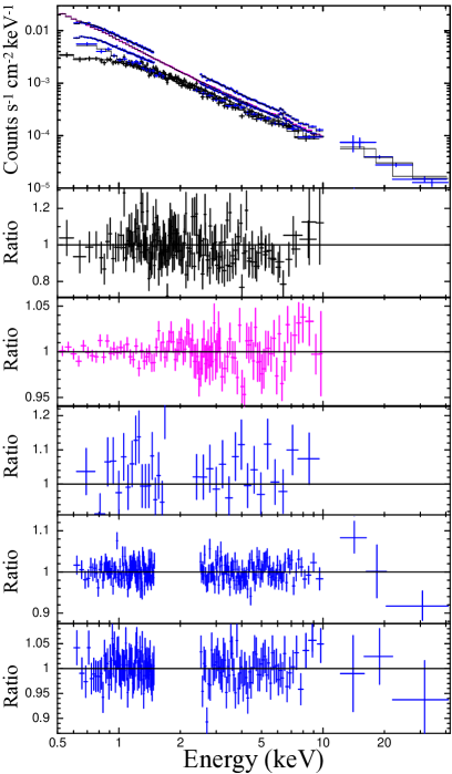
Figure 8: Fit to the ASCA (black), 2007 XMM-Newton (magenta) and Suzaku (blue) data. Bottom panels account for the data-model ratios.

Hitherto, ESO 511-G030 AGN has been observed by different facilities. Detailed studies on ASCA, Suzaku as well as the 2007 XMM-Newton exposure have already been published (e.g. Turner et al., 2001b; Ghosh & Laha, 2020), thus we will perform straight forward fits on these data to extract information on the spectral properties of ESO 511-G030 in previous years.
We tested our Model C, adopting the same fitting procedure described in previous Sect 4.3 and, slightly modifying the model when needed.
As clearly shown in Fig. 1, all archival exposures have larger fluxes than the data in 2019 and different spectral shapes, especially in the soft band. For this reason, we fitted separately ASCA, all the SUZAKU observations and XMM-Newton data. Concerning SUZAKU, the additional cross-calibration constant (k) was used for the XIS and PIN data.
Interestingly, our baseline Model C failed in reproducing all the archival spectra and additional components to this model are needed. In particular, a neutral absorption was required by ASCA data for which no relativistic reflection was necessary. For the SUZAKU data, instead, we added a single black body (bb) component to account for the soft-excess observed below $\displaystyle\sim$1 keV, while two bbs were added to fit the 2007 XMM-Newton exposure (see also Ghosh & Laha, 2020). These steps yielded the fits in Fig. 8 and in Table 3 we report the corresponding best-fit values.

Table 3: Parameters derived adapting the baseline Model C on the archival data. The L39 stands for the luminosity in units of 10³⁹ ergs s^-1 and D₁₀ is the distance in units of 10 kpc.

Mission	Comp.	Par.	Visit 1	Visit 2	Visit 3	Units
ASCA	tbabs	NH	1.0$\displaystyle\pm$0.2			$\displaystyle\times$1021 cm-2
	Borus	$\displaystyle\log\rm N_{H}$	¿23.1
		Norm	1.6$\displaystyle\pm$1.5			$\displaystyle\times 10^{-2}$ ph keV-1 cm-2 s-1
	power-law	$\displaystyle\Gamma$	1.91$\displaystyle\pm$0.08
		E${}_{\rm c}\dagger$	500			keV
		Norm	3.9$\displaystyle\pm$0.3			$\displaystyle\times 10^{-3}$ ph keV-1 cm-2 s-1
	$\displaystyle\chi^{2}$/d.o.f.		360/403
	p.null		0.9
	Flux${}_{\rm 0.5-2\leavevmode\nobreak\ keV}$		6.0$\displaystyle\pm$0.1			$\displaystyle\times 10^{-12}$ erg cm-2 s-1
	Flux${}_{\rm 2-10\leavevmode\nobreak\ keV}$		14.0$\displaystyle\pm$0.5			$\displaystyle\times 10^{-12}$ erg cm-2 s-1
XMM-Newton	bb	Tbb	180$\displaystyle\pm$15			eV
		Norm	3.2$\displaystyle\pm$0.4			$\displaystyle\times$10-5 L39
	bb	Tbb	75$\displaystyle\pm$10			eV
		Norm	1.0$\displaystyle\pm$0.2			$\displaystyle\times$10-4 L39
	relxill	rin	25${}^{+12}_{-20}$			Rg
		$\displaystyle\log\xi$	1.5$\displaystyle\pm$0.2
		Norm	1.8$\displaystyle\pm$0.6			$\displaystyle\times$10-5 ph keV-1 cm-2 s-1
	Borus	$\displaystyle\log\rm N_{H}$	23.8$\displaystyle\pm$0.3
		Norm	3.0$\displaystyle\pm$0.6			$\displaystyle\times 10^{-3}$ ph keV-1 cm-2 s-1
	power-law	$\displaystyle\Gamma$	1.88$\displaystyle\pm$0.02
		Norm	6.5$\displaystyle\pm$0.1			$\displaystyle\times 10^{-3}$ ph keV-1 cm-2 s-1
	$\displaystyle\chi^{2}$/d.o.f.		180/160
	p.null		0.2
	Flux${}_{\rm 0.5-2\leavevmode\nobreak\ keV}$		15.0$\displaystyle\pm$0.5			$\displaystyle\times 10^{-12}$ erg cm-2 s-1
	Flux${}_{\rm 2-10\leavevmode\nobreak\ keV}$		20.0$\displaystyle\pm$0.5			$\displaystyle\times 10^{-12}$ erg cm-2 s-1
SUZAKU	bb	Tbb	84$\displaystyle\pm$5	85$\displaystyle\pm$6	115$\displaystyle\pm$15	eV
		Norm	1.3$\displaystyle\pm$0.8	1.4$\displaystyle\pm$0.3	1.1$\displaystyle\pm$0.3	$\displaystyle\times$10-4 L39
	relxill	rin	-	¿2	¿10	Rg
		$\displaystyle\log\xi$	¿1.2	2.7$\displaystyle\pm$0.2	2.9$\displaystyle\pm$0.2
		Norm	0.85$\displaystyle\pm$55	0.75$\displaystyle\pm$0.35	2.1$\displaystyle\pm$1.2	$\displaystyle\times 10^{-5}$ ph keV-1 cm-2 s-1
	Borus	$\displaystyle\rm\log N_{\rm H}$	22.7$\displaystyle\pm$0.4	23.7$\displaystyle\pm$0.2	23.4$\displaystyle\pm$0.5
		Norm	2.0$\displaystyle\pm$1.0	2.1$\displaystyle\pm$0.4	2.3$\displaystyle\pm$0.4	$\displaystyle\times 10^{-2}$ ph keV-1 cm-2 s-1
	power-law	$\displaystyle\Gamma$	1.77$\displaystyle\pm$0.02	1.80$\displaystyle\pm$0.02	1.85$\displaystyle\pm$0.02
		Ec	500$\displaystyle\dagger$	¿120	$\displaystyle>$450	keV
		Norm	3.35$\displaystyle\pm$0.4	5.0$\displaystyle\pm$0.1	7.4$\displaystyle\pm$0.3	$\displaystyle\times 10^{-3}$ ph keV-1 cm-2 s-1
	const	k	-	1.3$\displaystyle\pm$0.10	1.16$\displaystyle\pm$0.08
	$\displaystyle\chi^{2}$/d.o.f.		312/306	1527/1437	1017/967
	p.null		0.42	0.04	0.097
	Flux${}_{\rm 0.5-2\leavevmode\nobreak\ keV}$		8.2$\displaystyle\pm$0.4	11.7$\displaystyle\pm$0.3	21.0$\displaystyle\pm$0.7	$\displaystyle\times 10^{-12}$ erg cm-2 s-1
	Flux${}_{\rm 2-10\leavevmode\nobreak\ keV}$		13.0$\displaystyle\pm$0.5	19.1$\displaystyle\pm$0.3	27.7$\displaystyle\pm$0.4	$\displaystyle\times 10^{-12}$ erg cm-2 s-1

Apart from the 1999 absorption event observed in the ASCA data due to matter with constant N_H=1.2$\displaystyle\pm$0.3 $\displaystyle\times$10²¹ cm^-2, ESO 511-G030 archival spectra are consistent with a variable power-law that is, on average, softer than in 2019 ($\displaystyle\Delta\Gamma\sim 0.2$). The continuum flux in the 2-10 keV energy range is up to a factor of $\displaystyle\sim$6 larger than in 2019 while the soft X-ray flux in the 0.5-2 keV range is even larger, up to a factor of $\displaystyle\sim$10. The large changes in the soft flux can be ascribed to the presence(lack) of the soft-excess component. The soft-excess clearly plays a major role in shaping the soft band in the 2007 XMM-Newton and 2011 SUZAKU observations.
The relativistic reflection observed in these archival observations is about $\displaystyle\sim$10 times larger than the one inferred in 2019, in agreement with the hot reflection responding to the primary changes. On the other hand, the reflected spectrum due to cold matter and also contributing to the Fe K$\displaystyle\alpha$ has, has a more constant behaviour across the years. Values derived for the normalisation the BorusK/L tables are, in fact, rather constant among the epochs. Thus, to a lower(higher) primary flux would correspond a larger(smaller) reflection fraction. Finally, the Compton-thin nature of the reprocessor in ESO 511-G030 is further confirmed by this data.

6 The Swift Monitoring campaign

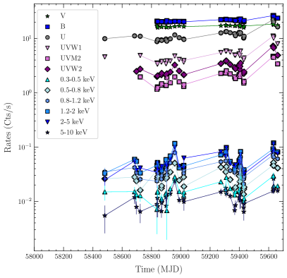
Figure 9: Multi filter light curves derived from 2018 up to 2022 for ESO 511-G030 usingSwift -XRT and -UVOT. Until the end of 2021 (MJD¡59580), after which a moderate increase of the ultraviolet emission can be observed, the optical-UV curves can be highly affected by the host emission. We notice that to quantify the actual amplitude of the optical-UV emission an estimate of the contribution of the host galaxy is required (see Sec 6.1).

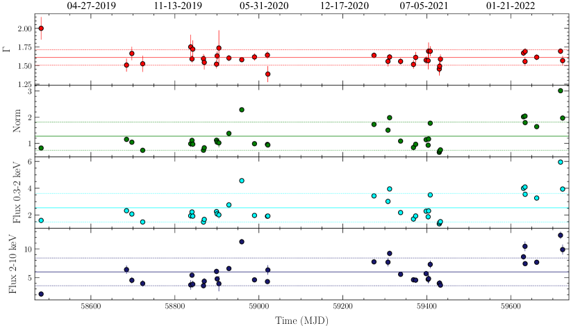
Figure 10: Best fit parameters and fluxes in the 0.3-2 (Soft) and 2-10 keV (hard) bands derived from Swift. Straight solid lines account for the mean value of the parameter while dotted lines represent the corresponding standard deviation. Fluxes are in units of $\displaystyle\rm 10^{-12}erg\leavevmode\nobreak\ cm^{-2}\leavevmode\nobreak\ s^{-1}$.

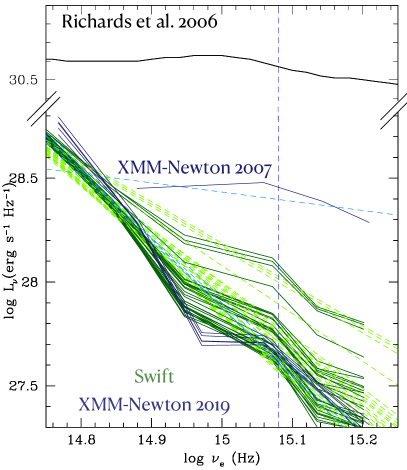
Figure 11: ESO 511-G030 optical/UV SEDs derived using XMM-Newton (blue) and Swift data (dark green). The corresponding least squares fits are showed as straight dashed lines. The solid thick black line is the average SED by Richards et al. (2006) for type-1 objects in the SDSS. The vertical dashed line is at $\displaystyle\log\nu_{*}=15.08$, corresponding to 2500Å. We notice the remarkable change in spectral shape from the 2007 observation versus the later ones.

We present here Swift X-ray and ultraviolet data that were taken in the context of two different observational campaigns, one of which is still ongoing, performed between 2020 and the present year. The objective of the campaigns is to keep track of the broadband properties of ESO 511-G030 and, possibly, observe a revenant soft-excess. Up to Fall 2021, however, the source flux state has been consistent with the one observed on 2019 with XMM-Newton and NuSTAR. In Fig. 9, we show the light curves derived for different X-ray bands (0.3-0.5, 0.5-0.8, 0.8-1.2, 1.2-2, 2-5 and 5-10 keV) and optical-UV filters (which are possibly dominated by the host galaxy). The Swift-XRT data show a min-to-max variability of about a factor of 5 across light curve. Once converted into fluxes, both X-rays and UVs are about a factor of $\displaystyle\sim$10 fainter than in the XMM-Newton observation of 2007, thus ESO 511-G030 as observed with Swift appears to be an extension of the quiescent state of ESO 511-G030 observed during 2019. By analysing the Swift spectra, our main objective was to establish whether a simple power-law component (plus Galactic absorption) was enough to explain the data. Our test, confirmed that a simple power-law well represents the 0.3-10 keV energy range of our source and no additional components are required. In Table 5 the inferred best-fit quantities are listed and the corresponding best-fit values are showed as a function of the observing time in Fig. 10. Swift data are consistent with a fairly flat spectral shape of $\displaystyle\Gamma$=1.62$\displaystyle\pm$0.09 and only small variability is observed in the power-law normalisation. This may suggest the source still remains in a quiescent state with no soft excess awakening.
To test whether the soft-excess was or not present in XRT spectra, we used all the observations quoted in Table A.1 to produce the stacked spectrum of ESO 511-G030. The obtained spectrum has no signature of this component. A simple power-law absorbed by the Galaxy ($\displaystyle\Gamma$=1.62$\displaystyle\pm$0.02) is in fact enough to account for the data ($\displaystyle\chi^{2}$=337 for 339 d.o.f.), this ruling out any additional component. The Swift fluxes in the 0.5-2 and 2-10 keV bands are compatible with what was observed during the 2019 XMM-Newton/NuSTAR monitoring campaign with F${}_{\rm 0.5-2\leavevmode\nobreak\ keV}$=(2.18$\displaystyle\pm$0.02)$\displaystyle\times 10^{-12}$ erg cm^-2 s^-1and F${}_{\rm 2-10\leavevmode\nobreak\ keV}$=(5.1$\displaystyle\pm$0.1)$\displaystyle\times 10^{-12}$ erg cm^-2 s^-1. Moreover, the stacked spectrum does not show any evidence of a Fe K$\displaystyle\alpha$ emission line. The lack of this feature can be likely explained by the coupled effects of the source low flux and the small effective area of the Swift-XRT telescope in the hard X-rays.
Finally, we notice that the last four Swift exposures of ESO 511-G030 were consistent with a flux increase of the source in both the X-ray and ultraviolet energy bands.

7 Relation between X-rays and UVs

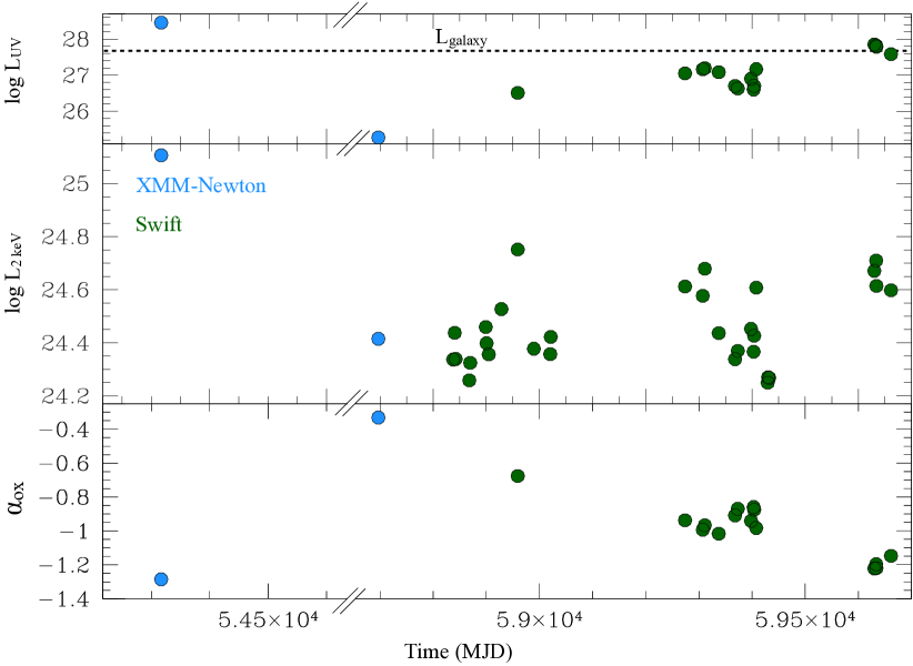
Figure 12: Light curves for the AGN luminosity at 2500 Å, at 2 keV, and the inferred $\displaystyle\alpha_{\rm OX}$. Blue dots identify values derived using XMM-Newton observations while in green the same quantities were estimated using Swift. The dashed horizontal line accounts for the adopted host galaxy luminosity at 2500 Å . Finally, both L_UV and L${}_{\rm 2\leavevmode\nobreak\ keV}$ are in units of erg s^-1 Hz^-1.

A viable way to quantify the actual relation between X-rays and UVs is provided by the $\displaystyle\alpha_{OX}$ parameter. The non-linear relation between the UV and X-ray luminosity in AGNs was discovered in late 1970s by Tananbaum et al. (1979) and several other authors investigating into the physical meaning of such a relation (e.g. Tananbaum et al., 1986; Zamorani et al., 1981; Vagnetti et al., 2010; Martocchia et al., 2017; Chiaraluce et al., 2018) and its implication in a cosmological framework (e.g. Risaliti & Lusso, 2015; Lusso & Risaliti, 2016, 2017; Lusso et al., 2020; Bisogni et al., 2021). Optical and ultraviolet data simultaneous with X-ray information are available for both XMM-Newton and Swift. For the 2007 XMM-Newton observation, only four OM filters are available (B, UVW1, UVM2, UVW2) while all of them were used in the 2019 monitoring campaign (V, B, U, UVW1, UVM2 and UVW2 at 5235Å, 4050Å, 3275Å, 2675Å, 2205Å, 1894Å, respectively). Swift-XRT observations are accompanied by one to six UVOT filters (V, B, U, UVW1 , UVM2 , UVW2 at 5468Å, 4392Å, 3465Å, 2600Å, 2246Åand 1928Å, respectively), this providing rich information on the UV continuum slope. We then derived the X-ray luminosity at 2 keV in order to compute the $\displaystyle\alpha_{OX}$ values. We relied on our best-fit to the EPIC-pn spectra discussed in Sect. 4 and 5 while the XRT spectra were modelled with a simple power-law with Galactic absorption, see Appendix A.

The total (AGN+galaxy) luminosity at $\displaystyle\log\nu_{*}=15.08$, corresponding to $\displaystyle\lambda$ = 2500Å, was estimated at each epoch as an interpolation between the data in the closest filters, which for these observations are UVW1 and UVM2. We computed the optical-ultraviolet spectral energy distributions (SEDs), to get an estimate of the host galaxy fraction at $\displaystyle\nu_{*}$, which may be significant, and of the AGN luminosity, $\displaystyle L_{UV}$, following the prescriptions by Vagnetti et al. (2013). We assumed each optical/UV SED in Fig. 11 to be the sum of an AGN spectrum, proportional to the average SED by Richards et al. (2006) with a typical slope $\displaystyle\alpha_{AGN}=-0.57$ (with $\displaystyle F_{\nu}\sim\nu^{\alpha_{AGN}}$), and a host galaxy contribution whose spectrum was modelled with a typical slope $\displaystyle\alpha_{galaxy}=-3$ (see e.g., Lusso et al. 2010; Vagnetti et al. 2013). The host galaxy fraction $\displaystyle f_{g}$ at $\displaystyle\nu_{*}$ was then derived at each epoch as a function of the sole spectral index. Indeed, expressing the total luminosity as $\displaystyle L=L_{*}[f_{g}(\nu/\nu_{*})^{-3}+(1-f_{g})(\nu/\nu_{*})^{-0.57}]$, the spectral index in $\displaystyle\nu_{*}$ is then equal to $\displaystyle\alpha=[d\log L/d\log\nu]_{\nu=\nu_{*}}=-3f_{g}-0.57(1-f_{g})$. The fraction $\displaystyle f_{g}$ was thus estimated inverting the previous relation as $\displaystyle f_{g}=-(0.57+\alpha)/2.43$. Therefore, when $\displaystyle f_{g}$ tends to zero then the slope $\displaystyle\alpha$ tends to -0.57, as per the Richards et al. (2006) AGN SED, while when $\displaystyle f_{g}=1$ $\displaystyle\alpha$ tends to -3, consistent with a pure host galaxy spectrum.
The monochromatic fluxes for the optical and ultraviolet filters were computed by converting the observed rates using the appropriate conversion factors. The spectral index was derived by least squares on these data. Figure 11 shows the optical-ultraviolet SEDs for the XMM-Newton and Swift observations. From 2007 to recent pointings, the ESO511-G030 SEDs underwent dramatic spectral changes. The optical/UV ESO 511-G030 SEDs appear quite steep with the exception of the 2007 exposure and those from Swift in 2022. The corresponding spectral index lies in the range between -2.7 and -3. These values are far steeper than the more typical slope of -0.57 derived from the average spectral energy distribution of a statistically significant number of AGNs by Richards et al. (2006) around $\displaystyle\nu_{*}$. The variation in the SEDs suggests that the nuclear emission changes, while a substantial constant contribution from the host galaxy is also present. In particular, the steep slopes derived for the observations taken after 2019 but before 2022 can be ascribed to the dominant shape of the host galaxy. The host galaxy luminosity at 2500Å is then defined as the average value of its estimates at the different epochs, which is found to be $\displaystyle\log L_{galaxy}=27.68$ (erg s^-1 Hz^-1), with a small dispersion, $\displaystyle\sigma=0.05$. This average value was then subtracted from the total luminosity at 2500Å to obtain the AGN luminosity $\displaystyle L_{UV}$ at each epoch. This luminosity $\displaystyle L_{UV}$ was often smaller than the host galaxy luminosity, as shown in the top panel of Fig. 12. For most observations, the ratio between the AGN and the total monochromatic luminosity (AGN+host) is in the range 0-50%. In many cases, the SED slope is $\displaystyle\lesssim-3$, the AGN fraction is negligible, and thus not plotted in Figs 12 and 13. On the opposite, the SED of the 2007 archival observation is flatter than the one by Richards et al. (2006) with $\displaystyle\alpha=-0.44$, thus, for this observation, we assumed the total monochromatic luminosity at 2500Å to be due to the AGN only.
The $\displaystyle\alpha_{OX}$ derived for our source can be also compared with the well-known $\displaystyle L_{UV}-\alpha_{OX}$ anti-correlation (Vignali et al., 2003; Just et al., 2007; Vagnetti et al., 2010). Fig. 13 shows the track of ESO 511-G030 in the $\displaystyle\log L_{UV}-\alpha_{OX}$ plane.

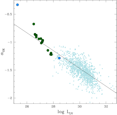
Figure 13: The ESO 511-G030 $\displaystyle\alpha_{\rm OX}$ estimates comparing them with the sample by Chiaraluce et al. (2018). The solid black line represents $\displaystyle{\rm logL_{\rm UV}-\alpha_{ox}}$ linear relation as derived in the same work.The $\displaystyle\alpha_{\rm OX}$ computed of ESO 511-G030 shows significant variability in agreement with the significant drop in the OM data showed in Fig. 1.

8 Ultraviolet to X-ray modelling

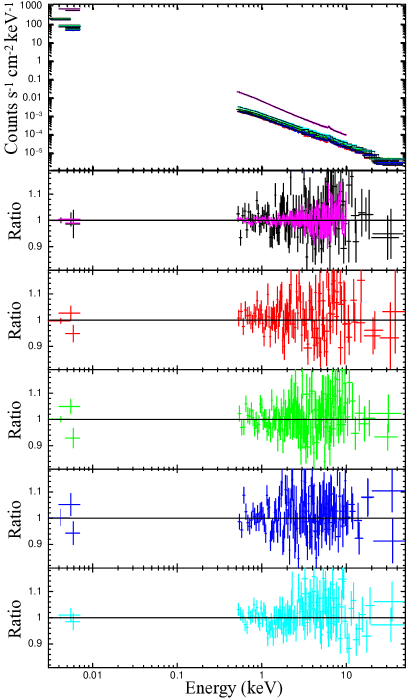
Figure 14: AGNSED reproducing the 2019 campaign and the archival XMM-Newton exposure (magenta). In bottom panels are shown data-model ratios for each datasets.

In accordance with previous Sect. 6, the multi wavelength properties of ESO 511-G030 varied dramatically on time. In 2007, in fact, the source ultraviolet-to-X-rays was consistent with the one of a bare Type 1 AGN. Later, once re-observed in 2019, neither the UVs nor the X-rays where compatible with their historical fluxes. Moreover, the ultraviolet emission which in 2007 was fully ascribable to the accretion process, turned out to be galaxy dominated, with only a few percent of the flux being due to the AGN.
To better understand the interplay among the different emission components in ESO 511-G030 across the years, we modelled the XMM-Newton spectrum taken in 2007 and those obtained in 2019. At this stage we included the corresponding OM data and tested AGNSED, (Kubota & Done, 2018). This models allows us to self-consistently reproduce the UV-to-X-ray spectra of ESO 511-G030. In accordance with Done et al. (2012), AGNSED accounts for three distinct emitting regions: an outer standard disc region; a warm Comptonising corona; and the inner hot Comptonising plasma. The flow is radially stratified and emits as a standard disc black body from R_out to R_warm, as warm Comptonisation from R_warm to R_hot (adopting the passive disc scenario by Petrucci et al., 2018) and, below R_hot down to R_ISCO as the typical hot Comptonisation component. We thus tested the model:

$$\rm tbabs_{G}\times redden\times(galaxy+AGNSED+relxillcp+Borus).\\$$ (1)

The tbabs_G was fixed to the value N_H=4.33$\displaystyle\times 10^{20}$ cm^-2 (HI4PI Collaboration et al., 2016) while the redden component fixed to a value of E(B-V)=0.056, in agreement with Schlafly & Finkbeiner (2011). We tested this model by fitting each observation separately and, within AGNSED we allowed the photon indices of the warm and hot coronae to vary as well as R_hot and R_warm. The hot coronal temperature was fixed to 100 keV to fit the 2007 data because there is no constraint above 10 keV, while it was left free to vary in the 2019 data. The warm coronal temperature was computed in both the datasets. We used a co-moving distance of 96 Mpc (derived from the redshift and adopted the mass for the SMBH in ESO 511-G030 by Ponti et al. (2012). Relxillcp and Borus (borus11_v190815a.fits), both accounting for a Comptonised continuum, were set similarly to what described in previous Sect. 4.2. These different flavours of relxill and Borus were used in order to tie the model parameters accounting for a Comptonised continuum (e.g. kT_e instead of E_cut) with the corresponding parameters in AGNSED, which assumes an underlying Comptonised continuum and not simply a cut-off power law. In the fit procedure we assumed the spin of the central SMBH to be maximally rotating in both relxillcp and AGNSED and the same disc inclination of 30° was also assumed. Then within AGNSED the upper limit of the scale height for the hot Comptonisation component, HTmax was set to be 10 R_g, which mimics a spherical Comptonisation region of similar radius. On the other hand, in relxillcp we set the emissivity profile to its default value of 3. The inner radius for the relxillcp reflection is fixed to R_hot. This assumption is discussed later. Then the outer disc radius was set to be the same (R_out=400 R_g) between the model component AGNSED and relxillcp. After preliminary tests, we fixed the relxillcp parameter R_in to 100 R_g as it could not be constrained in the 2019 data. Finally, we added a galaxy template accounting for the host galaxy (matching the morphological type of ESO 511-G030, i.e. Sc, Lauberts, 1982) contributing to the UV flux. The table was computed following Ezhikode et al. (2017) and included within XSPEC as a template named hostpol (Polletta et al., 2007). We notice that our galaxy model has a spectral shape between 3-10 eV of $\displaystyle\sim\Gamma$=4. This shape is fully consistent with our assumption in previous Sect. 7 for the host galaxy. We tied the normalisation of hostpol across the five spectra.
This procedure led us to the best-fit and model to data ratios shown in Fig. 14. The fit information as well as the corresponding yielded quantities are quoted in Table 4.

Table 4: Best-fit parameters derived adopting AGNSED on the XMM-Newton 2007 exposure and obs. 3 from the 2019 monitoring campaign. The symbol $\displaystyle\star$ is used for those values that were kept fixed in the fitting procedure

Comp.	Par.	Obs. 1	Obs. 2	Obs. 3	Obs. 4	Obs. 5	2007	units
Galaxy	Norm	4.5$\displaystyle\pm$1.5					-	$\displaystyle\times 10^{3}$
relxillcp	rin	100$\displaystyle\star$	100$\displaystyle\star$	100$\displaystyle\star$	100$\displaystyle\star$	100$\displaystyle\star$	30$\displaystyle\pm$15	Rg
	$\displaystyle\log\xi$	1.6$\displaystyle\pm$0.2	1.7$\displaystyle\pm$0.2	1.5$\displaystyle\pm$0.2	1.4$\displaystyle\pm$0.3	1.6$\displaystyle\pm$0.1	1.2$\displaystyle\pm$0.1
	Norm	¡2.0	1.2$\displaystyle\pm$0.8	2.1$\displaystyle\pm$0.7	¡1.7	4.0$\displaystyle\pm$1.0	25$\displaystyle\pm$1	$\displaystyle\times 10^{-6}$ ph keV-1 cm-2 s-1
Borus	Norm	1.8$\displaystyle\pm$0.3	1.9$\displaystyle\pm$0.4	1.6$\displaystyle\pm$0.4	1.8$\displaystyle\pm$0.4	1.7$\displaystyle\pm$0.3	(3.7$\displaystyle\pm$0.1)	$\displaystyle\times 10^{-3}$ ph keV-1 cm-2 s-1
	$\displaystyle\rm\log N_{H}$	23.2$\displaystyle\pm$0.2	23.2$\displaystyle\pm$0.2	23.4$\displaystyle\pm$0.2	23.2$\displaystyle\pm$0.1	23.2$\displaystyle\pm$0.2	23.7$\displaystyle\pm$0.3	1/(cm-2)
agnsed	$\displaystyle\log\dot{m}$	-2.73$\displaystyle\pm$0.12	-2.71$\displaystyle\pm$0.11	-2.66$\displaystyle\pm$0.06	-2.73$\displaystyle\pm$0.08	-2.56$\displaystyle\pm$0.02	-1.65$\displaystyle\pm$0.01
	$\displaystyle\Gamma_{\rm hot}$	1.75$\displaystyle\pm$0.02	1.75$\displaystyle\pm$0.02	1.76$\displaystyle\pm$0.02	1.75$\displaystyle\pm$2	1.76$\displaystyle\pm$0.01	1.91$\displaystyle\pm$0.02
	kThot	60${}^{+10}_{-25}$	70${}^{+10}_{-40}$	¿10	¿30	¿20	100$\displaystyle\dagger$	keV
	Rhot	39$\displaystyle\pm$5	38$\displaystyle\pm$6	42$\displaystyle\pm$3	40$\displaystyle\pm$3	41$\displaystyle\pm$3	27$\displaystyle\pm$1	Rg
	$\displaystyle\Gamma_{\rm warm}$	¡2.56	¡2.6	¡2.7	¡2.9	¡2.7	2.64$\displaystyle\pm$0.03
	kTwarm	0.16$\displaystyle\pm$0.06	0.22$\displaystyle\pm$0.07	0.20$\displaystyle\pm$0.09	0.23$\displaystyle\pm$0.07	¡0.3	0.17$\displaystyle\pm$0.02	keV
	Rwarm	¡52	¡54	¡52	50$\displaystyle\pm$5	¡57	150$\displaystyle\pm$2	Rg
	$\displaystyle\chi^{2}$/d.of.	280/260	290/256	310/266	320/287	380/331	200/165
	p.null	0.2	0.1	0.03	0.1	0.05	0.04

According to these fits, the SED of ESO 511-G030 varied dramatically from 2007 to 2019 as for the Eddington ratio that varied from a value of L/L${}_{\rm Edd}\sim$2% (in the 2007 spectrum soft-excess+power-law), to a rather low and radiatively inefficient value of $\displaystyle\sim$0.2% in 2019. The standard picture assumed within AGNSED i.e. the presence of a hot plasma (for R between R_isco and R${}_{\rm hot}\sim$27 R_g), a warm one (from R_hot to R${}_{\rm warm}\sim$150 R_g) and an accretion disc radially segregated agrees with the 2007 XMM-Newton observation. As said before, in our model the reflection is produced beyond R_hot. However in AGNSED a warm-corona is present between R_hot and R_warm and the standard disc starts only beyond R_warm. While we believe that the impact on our best fit results should be limited, our modelling does not take into account the presence of the warm corona in the reflection computation and thus does not provide a fully self-consistent physical picture of the emission emerging from ESO511-G030. To our knowledge the model REXCOR (Xiang et al., 2022) is the sole publicly available model that self-consistently computes the reflection spectrum from the combination of an outer standard disk and inner warm corona. However, this model cannot be extended to the UV energy range and cannot be used to fit simultaneously the OM data. Finally, the lack of a substantial soft-excess during the 2019 campaign leads to a different picture where the hot corona is now more extended than before and no clear indication of a warm Comptonising region is found. This warm region has shrunk and the disc already extends from $\displaystyle\lesssim$ 50 R_g, close to the hot component. The relativistic reflection component is less prominent and no constraints on the inner radius were obtained. The cold reflection component is compatible among the 2007 and 2019 data, in agreement with its distant origin from the central engine. Finally, the change for the hot and warm plasma components is also accompanied by the spectra evolving from a softer to a harder state, from $\displaystyle\Gamma$=1.91$\displaystyle\pm$0.03 to and average value of $\displaystyle\Gamma$=1.75$\displaystyle\pm$0.02.

9 Discussion and conclusions

We reported on the spectral and temporal properties of ESO 511-G030 that showed significant variability in both the optical-ultraviolet and X-ray. Our analysis revealed the ESO 511-G030 spectrum to be consistent with a primary power-law $\displaystyle\Gamma$=1.73$\displaystyle\pm$0.02 accompanied by a poorly constrained high energy roll over. The reflected flux we observed in the X-rays of ESO 511-G030 emerges from regions of different densities (Compton-thin and Compton-thick). In Fig. 7, we find the high energy spectrum to be dominated by reflection off a Compton-thin medium N${}_{\rm H}\sim 1.8^{23}$ cm^-2 that does not produce a relevant Compton-hump but accounts for a narrow Fe K$\displaystyle\alpha$ line. The relativistic reflection component reproduces the moderate broad shape of the same emission line and contributes to the overall spectral curvature.
Testing our Model C on archival data (our Sect. 5 and the work by Ghosh & Laha, 2020) revealed the primary component to be harder in 2019 than in past observations. These harder states were found in correspondence to lower flux levels, this suggesting the commonly observed softer-when-brighter trend. The reflected flux also varied; in particular the relativistic reflection is found to follow the variations of the primary emission (in agreement with this flux being released in the close surroundings of the central engine), while a less variable behaviour is observed for the cold reflection.
One of the main features of the 2019 observational campaign is the lack of a substantial soft-excess. A simple power-law, in fact, dominates the soft-to-hard X-ray spectrum of ESO 511-G030 at least from 2019. The lack of a soft-excess, or its negligible contribution to the overall emission spectrum of ESO 511-G030, is further supported by the analysis of the 2007 and 2019 excess variance spectra. Two different components are in fact needed to account for the 2007 F_var spectrum, one responsible for the changes in the X-ray continuum and a second accounting for the soft-excess. On the other hand, the F_var computed for the 2019 XMM-Newton exposures only requires a single component accounting for variance due to the nuclear continuum. It is worth noting that, while the F_var spectra of Fig. 4 sample slightly different timescales (see Sect. 3), we verified that when cutting the 2007 observation into shorter segments (so as to sample similar timescales as for the 2019 F_var spectra), a soft excess component still appears in the F_var of the lowest flux segment.
The absence of a strong soft-excess is quite unusual, since it is ubiquitously observed in AGNs (e.g. Piconcelli et al., 2005; Bianchi et al., 2009; Gliozzi & Williams, 2020). Note that ESO 511-G030 data do not require any absorbing component as also discussed in Laha et al. (2014).
The case of this Seyfert galaxy is peculiar and, we can only compare its behaviour with Mrk 1018. This other AGN had been studied in depth by Noda & Done (2018) who observed very different spectral shapes corresponding to different Eddington ratios. From a typical type 1 spectrum with a strong soft-excess, the source dimmed down, became harder and showed a weaker soft-excess. This spectral transition corresponded to a change in the Eddington ratio from L/L${}_{\rm Edd}\sim$2% to L/L${}_{\rm Edd}\sim$0.4% very similar to what is observed here for ESO 511-G030. As the soft excess is responsible for most of the ionising photons, the dramatic drop in the X-rays also led to the disappearance of the BLR, with this producing the ‘changing-look’ phenomenon. In other words, the presence(lack) of the soft-excess corresponded to a general softening(hardening) of the X-ray continuum emission with an accompanying dramatic change in the disc emission and a disappearance of the optical broad lines.
Similar to Mrk 1018, ESO 511-G030 had a dramatic change in its accretion rate passing from L/L${}_{\rm Edd}\sim$2% in 2007 down to L/L${}_{\rm Edd}\sim$0.2% in 2019. This dimming was also accompanied with a dramatic change in the UV SEDs (see Fig. 11 and Fig. 14), though it did not lead to a ’complete’ changing look process. An optical Floyds spectrum was, in fact, taken quasi-simultaneously with the XMM-Newton-NuSTAR campaign to check whether broad lines were present or not. From a quick comparison between the Floyds spectrum and an 6dF archival one taken in 2000, the H$\displaystyle\beta$ line does not disappear in 2019 with its velocity width being similar between the spectra (FWHM${}_{{\rm H}\beta}\sim 4500$ km s^-1, private communications with Keith Horne and Juan V. Hernández Santisteban)
The strong decrease of the accretion rate between 2007 and 2019 seems to be the crucial element to explain the observed spectral UV-X-ray behavior. Indeed this decrease naturally explains the strong decrease of the UV emission, see Fig.s  12 and 13. To 0th order, the decrease of the UV flux would also mean a decrease of the soft photons flux entering and cooling the hot corona. So we would expect an increase of the hot plasma temperature and a hardening of the X-ray spectrum with respect to 2007. The spectral hardening is observed and the absence of a stringent high energy cut-off signature in 2019 agrees with a large corona temperature, much larger than the usual values observed in Seyfert galaxies (e.g. Fabian et al., 2015, 2017; Tamborra et al., 2018; Middei et al., 2019). The absence of high signal high energy observations in the archives prevent any comparison with past observations that would help to support this scenario. But the strong decrease of the accretion rate could also explain the absence of the soft X-ray excess in 2019 at least in the case of the warm corona model. The observations agree with the warm corona being the upper layers of the accretion disc (Petrucci et al., 2018, and references therein). More importantly, to reproduce the soft X-ray spectral shape, simulations show that a large enough accretion power has to be released inside this warm corona and not in the accretion disc underneath (Różańska et al., 2015; Petrucci et al., 2020; Ballantyne, 2020). So if the accretion power becomes too low the warm corona cannot be energetically sustained. It is less obvious to understand why the soft X-ray excess would disappear if it is due to relativistically blurred ionised reflection. It is possible however that at low accretion rate the disc becomes more optically thin (or even recedes) producing less reflection as indeed observed in 2019.
However, other possible explanations for the lack of the soft-excess in ESO 511-G030 can be viable and new exposures, possibly performed during the awakening of this component, are mandatory in order to shed light onto the engine in this Seyfert galaxy. The increasing UV and X-ray fluxes observed by Swift in the first quarter of 2022 encourage us to ask for more observing time to, possibly, observe the revenant soft-excess of ESO 511-G030.

Appendix A The Swift-XRT observations

Results of the spectral analysis performed on the Swift-XRT observations belonging to our monitoring campaigns. Details are provided in Sect. 6.

Table 5: Best-fitted parameters as inferred from a spectral analysis of Swift-XRT spectra. Soft (0.3-2 keV) and hard (2-10 keV) fluxes are given in units of $\displaystyle\times 10^{-12}\rm erg\leavevmode\nobreak\ cm^{-2}\leavevmode\nobreak\ s^{-1}$.

Time	ObsID	$\displaystyle\Gamma$	FSoft	FHard	Cstat/d.o.f.
2018-12-29	03105115001	2.01$\displaystyle\pm$0.26	1.45$\displaystyle\pm$0.14	1.33$\displaystyle\pm$0.47	20/21
2019-07-20	00088915001	1.54$\displaystyle\pm$0.16	2.05$\displaystyle\pm$1.39	4.41$\displaystyle\pm$2.12	56/57
2019-08-02	00088915002	1.74$\displaystyle\pm$0.16	1.85$\displaystyle\pm$0.54	2.77$\displaystyle\pm$1.13	47/54
2019-08-28	00088915003	1.62$\displaystyle\pm$0.23	1.32$\displaystyle\pm$0.68	2.39$\displaystyle\pm$1.32	35/39
2019-12-20	00088915004	1.63$\displaystyle\pm$0.35	1.37$\displaystyle\pm$0.64	2.29$\displaystyle\pm$1.9	14/16
2019-12-23	00088915005	1.62$\displaystyle\pm$0.08	2.21$\displaystyle\pm$1.12	4.24$\displaystyle\pm$1.47	162/159
2019-12-25	00088915006	1.80$\displaystyle\pm$0.19	1.99$\displaystyle\pm$0.43	2.72$\displaystyle\pm$1.13	25/34
2020-01-20	00088915007	1.66$\displaystyle\pm$0.11	1.41$\displaystyle\pm$0.62	2.53$\displaystyle\pm$0.95	99/112
2020-01-21	00088915008	1.51$\displaystyle\pm$0.19	1.29$\displaystyle\pm$0.95	2.9$\displaystyle\pm$1.59	54/49
2020-02-20	00088915009	1.53$\displaystyle\pm$0.11	2.03$\displaystyle\pm$1.40	4.53$\displaystyle\pm$1.86	137/119
2020-02-21	00088915010	1.66$\displaystyle\pm$0.10	1.94$\displaystyle\pm$0.84	3.46$\displaystyle\pm$1.22	90/114
2020-02-25	00088915011	1.56$\displaystyle\pm$0.38	¡6.72	¡11.56	3/8
2020-03-20	00088915012	1.64$\displaystyle\pm$0.07	2.77$\displaystyle\pm$1.30	5.14$\displaystyle\pm$1.66	174/212
2020-04-20	00088915013	1.60$\displaystyle\pm$0.06	4.50$\displaystyle\pm$2.42	9.05$\displaystyle\pm$2.91	277/276
2020-05-20	00088915014	1.71$\displaystyle\pm$0.09	2.00$\displaystyle\pm$0.72	3.28$\displaystyle\pm$1.03	175/164
2020-06-20	00088915015	1.60$\displaystyle\pm$0.09	1.82$\displaystyle\pm$0.98	3.59$\displaystyle\pm$1.28	160/159
2020-06-21	00088915016	1.44$\displaystyle\pm$0.19	1.77$\displaystyle\pm$1.58	4.36$\displaystyle\pm$2.55	50/44
2021-03-01	00088915017	1.69$\displaystyle\pm$0.07	3.39$\displaystyle\pm$1.33	5.83$\displaystyle\pm$1.76	215/223
2021-04-03	00088915018	1.59$\displaystyle\pm$0.12	2.80$\displaystyle\pm$1.57	5.48$\displaystyle\pm$2.36	82/84
2021-04-07	00088915019	1.64$\displaystyle\pm$0.06	3.95$\displaystyle\pm$1.90	7.49$\displaystyle\pm$2.41	201/237
2021-05-03	00088915020	1.63$\displaystyle\pm$0.08	2.09$\displaystyle\pm$1.03	3.94$\displaystyle\pm$1.34	195/189
2021-06-03	00088915021	1.51$\displaystyle\pm$0.10	1.58$\displaystyle\pm$1.13	3.61$\displaystyle\pm$1.50	104/123
2021-06-08	00088915022	1.60$\displaystyle\pm$0.15	1.64$\displaystyle\pm$0.92	3.14$\displaystyle\pm$1.42	95/75
2021-07-03	00088915023	1.60$\displaystyle\pm$0.10	2.20$\displaystyle\pm$1.19	4.39$\displaystyle\pm$1.61	139/143
2021-07-08	00088915024	1.60$\displaystyle\pm$0.23	1.68$\displaystyle\pm$0.93	3.07$\displaystyle\pm$1.85	37/36
2021-07-09	00088915025	1.74$\displaystyle\pm$0.23	2.03$\displaystyle\pm$0.57	2.85$\displaystyle\pm$1.48	34/33
2021-07-13	00088915026	1.78$\displaystyle\pm$0.12	3.35$\displaystyle\pm$0.83	4.75$\displaystyle\pm$1.53	82/91
2021-08-03	00088915027	1.49$\displaystyle\pm$0.18	1.16$\displaystyle\pm$0.88	2.61$\displaystyle\pm$1.41	63/61
2021-08-04	00088915028	1.58$\displaystyle\pm$0.16	1.24$\displaystyle\pm$0.73	2.45$\displaystyle\pm$1.19	44/60
2021-08-06	00088915029	1.62$\displaystyle\pm$0.12	1.45$\displaystyle\pm$0.72	2.71$\displaystyle\pm$1.08	97/109
2022-02-20	00088915032	1.67$\displaystyle\pm$0.06	4.0$\displaystyle\pm$0.2	8.6$\displaystyle\pm$0.7	171/208
2022-02-23	00088915033	1.55$\displaystyle\pm$0.10	4.1$\displaystyle\pm$0.3	10.0$\displaystyle\pm$1.0	122/102
2022-02-24	00088915034	1.69$\displaystyle\pm$0.07	3.5$\displaystyle\pm$0.2	7.4$\displaystyle\pm$0.7	166/179
2022-03-23	00088915035	1.61$\displaystyle\pm$0.07	3.3$\displaystyle\pm$0.2	7.6$\displaystyle\pm$0.5	183/215