SDYN-GANs: Adversarial Learning Methods for Multistep Generative Models for General Order Stochastic Dynamics

Abstract

We introduce adversarial learning methods for data-driven generative modeling of the dynamics of $n^{th}$-order stochastic systems. Our approach builds on Generative Adversarial Networks (GANs) with generative model classes based on stable $m$-step stochastic numerical integrators. We introduce different formulations and training methods for learning models of stochastic dynamics based on observation of trajectory samples. We develop approaches using discriminators based on Maximum Mean Discrepancy (MMD), training protocols using conditional and marginal distributions, and methods for learning dynamic responses over different time-scales. We show how our approaches can be used for modeling physical systems to learn force-laws, damping coefficients, and noise-related parameters. The adversarial learning approaches provide methods for obtaining stable generative models for dynamic tasks including long-time prediction and developing simulations for stochastic systems.

Keywords: Adversarial Learning, Generative Adversarial Networks (GANs), Dimension Reduction, Reduced-Order Modeling, System Identification, Stochastic Dynamical Systems, Stochastic Numerical Methods, Generalized Method of Moments (GMM), Maximum Mean Discrepancy (MMD), Scientific Machine Learning.

1 Introduction

Learning and modeling tasks arising in statistical inference, machine learning, engineering, and the sciences often involve inferring representations for systems exhibiting non-linear stochastic dynamics. This requires estimating models that not only account for the observed behaviors but also allow for performing simulations or making predictions over longer time-scales. Obtaining stable long-time simulations and predictions requires data-driven approaches capable of learning structured dynamical models from observations.

Estimating parameters and representations for stochastic dynamics has a long history in the statistics and engineering community (Peeters and De Roeck, 2001; Hurn et al., 2007; Jensen and Poulsen, 2002; Kalman, 1960; Nielsen et al., 2000). This includes methods for inferring models and parameters in robotics (Olsen et al., 2002), orbital mechanics (Muinonen and Bowell, 1993), geology (Pardo-Igúzquiza, 1998), political science (King, 1998), finance (Kim et al., 1998), and economics (Cramer, 1989). One of the most prominent strategies for developing estimators is to use Maximum Likelihood Estimation (MLE) (Fisher and Russell, 1922; Hald, 1999) or Bayesian Inference (BI) (Gelman et al., 1995). For systems where likelihoods can be specified readily and computed tractably, estimators can be developed with asymptotically near optimal data efficiency (Wasserman, 2010). However, in general, specifying and computing likelihoods for MLE, especially for stochastic processes, can pose significant challenges in practice (Hurn et al., 2007; Sørensen, 2004). For Bayesian methods, this is further compounded by well-known challenges in computing and analyzing posterior distributions (Gelman et al., 1995; Smith and Roberts, 1993). For stochastic systems, this is also compounded by the high dimensionality of the ensemble of observations and data consisting of trajectories of the system.

As an alternative to MLE methods, we develop adversarial learning methods using discriminators/critics based on a generalization of the method-of-moments building on (Hansen, 1982; Gretton et al., 2012; Fortet and Mourier, 1953). We develop methods for learning models and estimating parameters using a generative modeling approach which compares samples of candidate models with the observation data. A notable feature of these sample-based adversarial methods is they is no longer require specification of likelihood functions. This allows for learning over more general classes of generative models. The key requirement now becomes identifying a collection of features of the samples that are sufficiently rich for the discriminators/critics to make comparisons with the observation data for model selection. We develop methods based on characteristic kernels and generalized moments for distinguishing general classes of distributions (Gretton et al., 2012; Fortet and Mourier, 1953).

We introduce adversarial learning approaches and training methods for obtaining representations of $n^{th}$-order stochastic processes using a class of generative models based on $m$-step stochastic numerical methods. For gradient-based learning with loss functions based on second-order statistics, and the high dimensional samples arising from trajectory observations, we develop specialized adjoint methods and custom backpropagation methods. Our approaches provide Generative Adversarial Networks (GANs) for learning representations of the non-linear dynamics of stochastic systems. We refer to the methods as Stochastic-Dynamic Generative Adversarial Neural Networks (SDYN-GANs).

2 Adversarial Learning

We develop adversarial learning approaches for the purpose of quantifying the differences between a collection of samples from candidate generative models from those of the training data. In adversarial learning a generative model $G(\cdot;\theta_{G})$ is learned in conjunction with a discriminative model $D(\cdot;\theta_{D})$. This can be viewed as a two-player game. The aim of the discriminator $D$ is to minimize errors in distinguishing a collection of samples of the generator from those of the training data. The aim of the generator is to produce samples of such good quality that the discriminative model is confused and would commit errors in being able to distinguish them from the training data, see Figure 1. Depending on the choices made for the loss functions, and the model classes of the discriminative and generative models, different types of divergences and metrics can be obtained. These choices impact how comparisons are made between the distribution of the generative model with the distribution of the training data. In practice, learning methods are sought that perform well using only samples from these distributions.

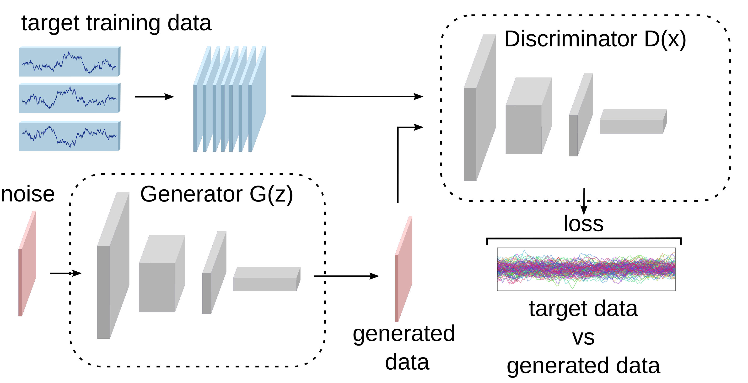
Figure 1: Adversarial Learning. A generative model $G(\cdot;\theta_{G})$ and discriminator/critic $D(\cdot;\theta_{D})$ are used to learn models from samples of the trajectory data. The $D$ is used in computing a loss comparing samples $\{\mathbf{\tilde{x}}_{i}\}_{i=1}^{\tilde{N}}$ generated by $G$ with the samples $\{\mathbf{x}_{i}\}_{i=1}^{N}$ of the training data.

2.1 Generative Adversarial Networks (GANs)

In the adversarial training of GANs, the first model $G$ is a neural network representing an implicit generative model denoted by $G(\mathbf{Z};\theta_{G})$ that generates samples from a random source $\mathbf{Z}$. The $\theta_{G}$ are the parameters of the model and $\mathbf{Z}$ denotes a random variable mapped under $G$ to generate samples $\tilde{\mathbf{x}}^{[i]}=G(\mathbf{Z}^{[i]};\theta_{G})$. The second model $D$ serves to distinguish how well a set of samples $\{\tilde{\mathbf{x}}^{[i]}\}_{i=1}^{\tilde{N}}$ generated by $G$ matches samples $\{\mathbf{x}^{[i]}\}_{i=1}^{N}$ with those in the training data set. Let the empirical distributions be denoted for the generator by $\tilde{\mu}_{G}$ and for the training data by $\tilde{\mu}_{\mathcal{D}}$. The discriminator/critic model is denoted by $D(\cdot;\theta_{D})$. The choices for the form of $D$ and for the loss functions $\ell$ determine how the comparisons are made between the empirical probability distributions of the two sets of samples, $\tilde{\mu}_{G},\tilde{\mu}_{\mathcal{D}}$. There are many ways to formulate GANs and related statistical estimators (Sriperumbudur et al., 2009; Goodfellow et al., 2016).

In the original formulation of GANs, the objective can be expressed as
$\theta_{D}^{*}=\arg\min_{\theta_{D}}J_{D}(\theta_{G},\theta_{D})$ with $J_{D}=\mathbb{E}_{(x,y)\sim p_{{\mbox{\tiny synth}}}}\left[-\log p_{\mbox{\tiny D}}(y|x;\theta_{D})\right]$, (Goodfellow et al., 2014, 2016). The $p_{{\mbox{\tiny synth}}}(x,y)=\frac{1}{2}p_{\mbox{\tiny data}}(x,y)+\frac{1}{2}p_{\mbox{\tiny model}}(x,y;\theta_{G})$ is the probability of a synthetic data distribution obtained by mixing the samples of the generator $\tilde{x}\sim p_{\mbox{\tiny model}}\sim\tilde{\mu}_{G}$ with the training data $x\sim p_{\mbox{\tiny data}}\sim\tilde{\mu}_{\mathcal{D}}$, (Goodfellow et al., 2016). The labels are assigned to the samples with $y=-1$ for the generated data samples and $y=+1$ for training data. For a given $\theta_{D}$, we let $D(x)=p_{\mbox{\tiny D}}(y=+1|x;\theta^{D})$ for the probability that the discriminator classifier assigns the sample $x$ to have the label $y=+1$. We then have $1-D(x)=p_{\mbox{\tiny D}}(y=-1|x;\theta_{D})$. With these choices and notation, the objective now can be expressed as $J_{D}=-\frac{1}{2}\mathbb{E}_{x\sim p_{{\mbox{\tiny data}}}}\left[\log(D(x))\right]-\frac{1}{2}\mathbb{E}_{x\sim p_{{\mbox{\tiny model}}}(;\theta_{G})}\left[\log(1-D(x))\right].$ The aim is for the generator to produce high quality samples so that even the optimal discriminator $\theta_{D}^{*}$ is confused and gives the value $D(x)=p_{\mbox{\tiny D}}(\cdot;\theta_{D}^{*})=1/2$.

The optimal generative model in this case has objective $\theta_{G}^{*}=\arg\min_{\theta_{G}}J_{G}(\theta_{G},\theta_{D}^{*}(\theta_{G}))$. When $J_{G}=-J_{D}$, this can be viewed as a two-player zero-sum game with cost function $\ell=J_{D}$ with $\theta_{D}^{*}$ and $\theta_{G}^{*}$ corresponding to the optimal strategies. If the objectives are fully optimized to the equilibrium, this would give the Jensen-Shannon (JS) Divergence $JS(\tilde{\mu}_{G(;\theta_{G})},\tilde{\mu}_{\mathcal{D}})$ (Lin, 1991) for comparing the empirical distributions of the generator $\tilde{\mu}_{G}$ and training data $\tilde{\mu}_{\mathcal{D}}$. The optimal generator would be $\theta_{G}^{*}=\arg\min_{\theta_{G}}JS(\tilde{\mu}_{G(;\theta_{G})},\tilde{\mu}_{\mathcal{D}})$, where $JS(\tilde{\mu}_{G},\tilde{\mu}_{\mathcal{D}})=\frac{1}{2}D_{KL}\left(\tilde{\mu}_{\mathcal{D}}\|\frac{1}{2}\left(\tilde{\mu}_{G}+\tilde{\mu}_{\mathcal{D}}\right)\right)+\frac{1}{2}D_{KL}\left(\tilde{\mu}_{G}\|\frac{1}{2}\left(\tilde{\mu}_{G}+\tilde{\mu}_{\mathcal{D}}\right)\right)$, with $D_{KL}$ the Kullback-Leibler Divergence (Cover and Thomas, 2006; Kullback and Leibler, 1951). In practice, to mitigate issues with gradient-learning, the zero-sum condition can be relaxed by using different loss functions in the objectives with $J_{G}\neq-J_{D}$. For example, $J_{G}=-\frac{1}{2}\mathbb{E}_{x\sim p_{{\mbox{\tiny model}}}(;\theta_{G})}\left[\log(D(x))\right]$ is used sometimes for the generator $G$ to improve the gradient (Goodfellow et al., 2016). Such formulations can result in other types of games with more general solutions characterized as Nash Equilibria or other stationary states (Nisan et al., 2007; Owen, 2013; Nash, 1951; Roughgarden, 2010).

GANs and other statistical estimators also can be formulated using discriminators/critics based on $J_{D}(\theta_{G},\theta_{D})=\mathbb{E}_{\tilde{\mu}_{G(;\theta_{G})}}\left[F(X^{\prime};\theta_{D})\right]-\mathbb{E}_{\tilde{\mu}_{\mathcal{D}}}\left[F(X;\theta_{D})\right]$ and $J_{G}=-J_{D}$ with
$\theta_{G}^{*}=\arg\min_{\theta_{G}}J_{G}(\theta_{G},\theta_{D}^{*}(\theta_{G}))$ and $\theta_{D}^{*}=\arg\min_{\theta_{D}}J_{D}(\theta_{G},\theta_{D})$. This objective can be viewed from a statistical perspective as yielding an Integral Probability Metric (IPM) (Sriperumbudur et al., 2009; Muller, 1997). The IPM can be expressed as
$\theta_{G}^{*}=\arg\min_{\theta_{G}}\max_{f\in\mathcal{F}}\left(\mathbb{E}_{\tilde{\mu}_{\mathcal{D}}}\left[f(X)\right]-\mathbb{E}_{\tilde{\mu}_{G(;\theta_{G})}}\left[f(X^{\prime})\right]\right)=\arg\min_{\theta_{G}}\max_{f\in\mathcal{F}}\ell(\theta_{G};f)=\arg\min_{\theta_{G}}\ell^{*}(\theta_{G})$, where $\mathcal{F}=\{f\;|\;\exists\theta_{D}\mbox{ s.t. }f=F(\cdot;\theta_{D})\}$ and $\ell^{*}(\theta_{G})=\max_{f\in\mathcal{F}}\ell(\theta_{G};f)$. In the case of $\mathcal{F}=\mbox{Lip-}1$, consisting of Lipschitz functions with $L\leq 1$, this results in $\ell^{*}(\theta_{G})=\max_{f\in{\small\mbox{Lip-}1}}\ell(\theta_{G};f)=\mathcal{W}^{1}\left(\tilde{\mu}_{G},\tilde{\mu}_{\mathcal{D}}\right)$. This follows by Kantorovich-Rubinstein Duality, where $\mathcal{W}^{1}$ is the Wasserstein-1 distance for the empirical measures $\tilde{\mu}_{G}$ and $\tilde{\mu}_{\mathcal{D}}$ (Villani, 2008). While Wasserstein distance provides a widely used norm for analyzing measures, in practice for training, it can be computationally expensive to approximate and can result in challenging gradients for learning (Mallasto et al., 2019).

As an alternative to these approaches, we use for IPMs a smoother class of discriminators, with $\mathcal{F}\subset\mathcal{H}$ with $\mathcal{H}$ a Reproducing Kernel Hilbert Space (RKHS) (Aronszajn, 1950; Berlinet and Thomas-Agnan, 2011). By choice of the kernel $k(\cdot,\cdot)$ we also can influence the features of the distributions that are emphasized during comparisons. We take $\mathcal{F}=\{f\in\mathcal{H}\;|\;\|f\|_{\mathcal{H}}\leq 1\}$ for the objective, $\theta_{G}^{*}=\arg\min_{\theta_{G}}\max_{f\in\mathcal{F}}\ell(\theta_{G};f)$, where $\ell(\theta_{G};f)=\mathbb{E}_{\tilde{\mu}_{\mathcal{D}}}\left[f(X)\right]-\mathbb{E}_{\tilde{\mu}_{G(;\theta_{G})}}\left[f(X^{\prime})\right]$.

The objective can be partially solved analytically to yield $\ell^{*}(\theta_{G})=\max_{f\in\mathcal{F}}\ell(\theta_{G};f)=\|\eta_{\mathbb{P}}-\eta_{\mathbb{Q}}\|_{\mathcal{H}}$, where $\eta_{\mathbb{P}}=E_{X\sim\mathbb{P}}\left[k(\cdot,X)\right]$, $\eta_{\mathbb{Q}}=E_{X^{\prime}\sim\mathbb{Q}}\left[k(\cdot,X^{\prime})\right]$ and $\|\cdot\|_{\mathcal{H}}$ is the norm of the RKHS (Sriperumbudur et al., 2010). Here, we take $\mathbb{P}=\tilde{\mu}_{\mathcal{D}}$ to be the empirical distribution of the training data and $\mathbb{Q}=\tilde{\mu}_{G}$ the empirical distribution of the generated samples. Characterizing the differences between the probability distributions in this way corresponds to the statistical approaches of Generalized Method of Moments (Hansen, 1982) and Maximum Mean Discrepancy (MMD) (Fortet and Mourier, 1953; Smola et al., 2006).

2.2 SDYN-GANs Adversarial Learning Framework for Stochastic Dynamics

We discuss our overall adversarial training approach for learning generative models for stochastic dynamics, and give more technical details in the later sections. Learning representations of stochastic dynamics capable of making long-time predictions presents challenges for direct application of traditional estimation methods not taking temporal aspects into account. This arises from the high dimensionality of trajectory data samples and in the need for stable models that can predict beyond the time duration of the observed dynamics. To obtain reliable learning methods requires making effective use of the special structures of the stochastic system and trajectory data. This includes Markovian conditions, probabilistic dependencies, and other properties.

While our approaches can be used more broadly, we focus here on learning generative models related to vector-valued Ito Stochastic Processes (Oksendal, 2000). This is motivated by systems with unknown features which can be modeled by solutions of Stochastic Differential Equations (SDEs) (Oksendal, 2000; Gardiner, 1985). From a probabilistic graphical modeling perspective (Wainwright and Jordan, 2008; Bishop, 2006; Sucar, 2015; Murphy, 2012), the high dimensional probability distributions associated with observations of trajectories can be factored. This allows for dependencies to be used to obtain more local models coupling the components over time greatly reducing the dimensionality of the problem. For obtaining generative models $G$ that are useful for prediction and long-time simulations, we develop generator classes based on stable $m$-step stochastic numerical integrators with learnable components (Kloeden and Platen, 1992). As we discuss in later sections, we motivate and investigate the performance of our methods by considering problems for physical systems and mechanics in $\mathbb{R}^{3}$. In this case, we can further refine the class of numerical discretizations to incorporate physical principles, such as approximate time-reversibility for the conservative contributions to the dynamics, fluctuation-dissipation balance, and other properties (Verlet, 1967; Gronbech-Jensen and Farago, 2013; Jasuja and Atzberger, 2022; Tabak and Atzberger, 2015; Trask et al., 2020; Lopez and Atzberger, 2022).

Figure 2: Decompositions for Training. We utilize for the trajectories the probabilistic dependence between the configurations $\mathbf{X}(t)$ to help facilitate learning models from the time series data (left). We develop different training protocols using (i) conditional statistics and (ii) marginal statistics. We also develop training methods for different trajectory durations $[0,\mathcal{T}]$ and sub-sampling over time-scales $\tau$ (right).

We develop Stochastic Dynamic Generative Adversarial Networks (SDYN-GANs), for learning generative models $G$ for sampling discretized trajectories, $\mathbf{X}^{[i]}=G(\mathbf{Z}^{[i]},\theta_{G})$. The $\mathbf{Z}^{[i]}$ denotes the sample of the noise source mapped under $G$ to generate the sample $\mathbf{X}^{[i]}$. The data samples can be expressed as $\mathbf{X}^{[i]}=\left(\mathbf{X}_{1}^{[i]},\ldots,\mathbf{X}_{N}^{[i]}\right)$ where $\mathbf{X}_{j}^{[i]}=\mathbf{X}^{[i]}(t_{j})$ are the temporal components. We learn generators $G$ having the form of $m$-step stochastic numerical integration methods $\mathbf{X}_{j}=\boldsymbol{\Psi}_{j-1}(\mathbf{X}_{j-1},\ldots,\mathbf{X}_{j-m},\boldsymbol{\omega}_{j-1};\mathbf{p})$ with initial conditions $\mathbf{X}_{0}=\mathbf{x}_{0}(\mathbf{p}),\ldots,\mathbf{X}_{m-1}=\mathbf{x}_{m-1}(\mathbf{p})$. The trainable term $\boldsymbol{\Psi}_{j-1}$ approximates the evolution of the stochastic dynamics from time-step $t_{j-1}$ to $t_{j}$ using information at times $t_{j-1},\ldots,t_{j-m}$. The numerical updates are randomized with samples $\boldsymbol{\omega}_{j-1}$ and have learnable parameters $\mathbf{p}$. In terms of $G(\mathbf{Z};\theta_{G})$, we will consider here primarily the case with $\mathbf{Z}=\{\boldsymbol{\omega}_{j}\}_{j}$ and $\theta_{G}=\mathbf{p}$. In the general case, $\mathbf{Z}$ can also include additional sources of noise and $\theta_{G}$ additional parameters. The use of $m$-step stochastic methods for our generative modeling allows for leveraging probabilistic dependencies to factor high dimensional trajectory data. Our $m$-step methods can be viewed as a variant of structural equations for probabilistic graphical modeling (Bishop, 2006; Murphy, 2012; Wainwright and Jordan, 2008; Ding et al., 2021), see Figure 2.

We use adversarial learning to train the generative model $G$ by using discriminators/critics $D$ to distinguish the samples generated by $G$ from those of the training data. We obtain generators by optimizing the loss $\theta_{G}^{*}=\arg\min_{\theta_{G}}\ell^{*}(\theta_{G})$, with $\ell^{*}(\theta_{G})=\ell(\theta_{G},\theta_{D}^{*}(\theta_{G}))$. This can be formulated many different ways corresponding to different divergences and metrics of the empirical distributions as we discussed in Section 2.1. We use losses $\hat{\ell}^{*}$ corresponding to Integral Probability Metrics (IPMs) of the form $\hat{\ell}^{*}(\theta_{G})=\hat{\ell}^{*}(\mathbb{P},\mathbb{Q})=\max_{f\in\mathcal{F}}\left(\mathbb{E}_{\mathbb{P}}\left[f(\mathbf{X})\right]-\mathbb{E}_{\mathbb{Q}}\left[f(\mathbf{X^{\prime}})\right]\right)$, where $\mathbb{P}$, $\mathbb{Q}$ denote the measures being compared. We take $\mathbb{P}=\tilde{\mu}_{\mathcal{D}},\mathbb{Q}=\tilde{\mu}_{G}$ and use $\mathcal{F}=\{f\in\mathcal{H}\;|\;\|f\|_{\mathcal{H}}\leq 1\}$, where $\mathcal{H}$ is a Reproducing Kernel Hilbert Space (RKHS) with kernel $k(\cdot,\cdot)$. With these choices, we can express the GANs and resulting IPM loss as $\hat{\ell}^{*}(\theta_{G})=\|\eta_{\mathbb{Q}}-\eta_{\mathbb{P}}\|_{\mathcal{H}}$, where $\eta_{\mathbb{P}}=\mathbb{E}_{\mathbb{P}}\left[k(\cdot,\mathbf{X})\right]$ and $\eta_{\mathbb{Q}}=\mathbb{E}_{\mathbb{Q}}\left[k(\cdot,\mathbf{X})\right]$. This can be viewed as embedding each of the measures as functions in the RKHS $\mathcal{H}$ (Saitoh and Sawano, 2016; Sriperumbudur et al., 2010). The characterization of their differences can be expressed as the $\mathcal{H}$-norm of their embedded representations. Since $k(\cdot,\mathbf{X})$ gives a collection of features, which under expectation generate generalized moments, this approach corresponds to Generalized Moments Methods (GMMs) (Hansen, 1982) and Maximum Mean Discrepancy (MMD) (Gretton et al., 2012; Fortet and Mourier, 1953; Smola et al., 2006).

In practice, to obtain more amenable losses for optimization and for computing gradients, we use a reformulation which squares the objective to obtain $\ell^{*}(\theta_{G})=\left(\hat{\ell}^{*}(\theta_{G})\right)^{2}=\|\eta_{\mathbb{P}}-\eta_{\mathbb{Q}}\|_{\mathcal{H}}^{2}=\mathbb{E}_{\mathbf{X}\sim\mathbb{P}}\left[k(\mathbf{X},\mathbf{X})\right]-2\mathbb{E}_{\mathbf{X}\sim\mathbb{P},\mathbf{X^{\prime}}\sim\mathbb{Q}}\left[k(\mathbf{X},\mathbf{X^{\prime}})\right]+\mathbb{E}_{\mathbf{X^{\prime}}\sim\mathbb{Q}}\left[k(\mathbf{X^{\prime}},\mathbf{X^{\prime}})\right]$. This is related to energy statistics (Székely and Rizzo, 2013) and the sample-based estimator developed in (Gretton et al., 2012). To find approximate minimizers for training $G$, we use Stochastic Gradient Descent (SGD) methods $\theta_{G}^{n+1}=\theta_{G}^{n}-\eta_{n}\hat{q}$, with learning rate $\eta_{n}$ and gradient estimators $\hat{q}\approx\nabla_{\theta_{G}}\ell^{*}(\theta_{G}^{n})$ based on mini-batches  (Robbins and Monro, 1951; Bottou et al., 1991; Bishop, 2006). We use variants incorporating momentum, such as ADAM and others (Kingma and Ba, 2014; Tieleman and Hinton, 2012; Lydia and Francis, 2019). To compute $\hat{q}$, we use the unbiased estimator of (Gretton et al., 2012) as part of the gradient approximation. We estimate gradients for the empirical loss using $\hat{q}=\nabla_{\theta_{G}}\tilde{\ell}^{*}(\theta_{G})$ where

$$\tilde{\ell}^{*}(\theta_{G})=\hskip 394.59578pt$$ (1)

$$\frac{1}{N(N-1)}\sum_{i\neq j}^{N}k\left(\mathbf{X}^{[i]},\mathbf{X}^{[j]}\right)-\frac{2}{NM}\sum_{i=1}^{N}\sum_{j=1}^{M}k\left(\mathbf{X}^{[i]},\mathbf{Y}^{[j]}\right)+\frac{1}{M(M-1)}\sum_{i\neq j}^{M}k\left(\mathbf{Y}^{[i]},\mathbf{Y}^{[j]}\right).$$

The samples of mini-batches have distributions $\mathbf{X}^{[i]}\sim\tilde{\mu}_{G}$ and $\mathbf{Y}^{[i]}\sim\tilde{\mu}_{\mathcal{D}}$.

The trajectory samples $\mathbf{X}^{[i]}=G(\mathbf{Z}^{[i]};\theta_{G})$ depend on $\theta_{G}$, which further requires methods for computing the contributions of the gradients $\nabla_{\theta_{G}}\mathbf{X}^{[i]}$. This can pose challenges since these gradients involve the $m-$step stochastic integrators when $\mathbf{p}\subset\theta_{G}$. This can become particularly expensive if using direct backpropagation based on book-keeping for forward evaluations of the stochastic integrators and the second-order statistics of $\tilde{\ell}^{*}$. This would result in prohibitively large computational call graphs. This arises from the high dimension of the trajectories $\mathbf{X}$ and the multiple dependent steps during generation. This is further compounded by the mini-batch sampling $\{\mathbf{X}^{[i]}\}_{i=1}^{n_{b}}$ and second-order statistics. As we discuss in the later Sections 4.2 and 4.3, we can address these issues by developing adjoint methods and custom backpropagation approaches specialized to utilize the structure of the loss functions. This allows us to compute efficiently the contributions of $\nabla_{\theta_{G}}\mathbf{X}^{[i]}$ to $\nabla_{\theta_{G}}\tilde{\ell}^{*}$ to obtain the gradient estimates needed for training.

We also introduce and investigate for SDYN-GANs training protocols utilizing the trajectory data in a few different ways to compare the underlying probability distributions, see Figure 2. This includes comparisons using (i) distributions over the entire trajectory, (ii) marginal distributions over trajectory fragments, and (iii) conditional distributions over trajectory fragments. We develop the following training approaches for $n^{th}$-order stochastic systems

• Full-Trajectory Method (full-traj): Samples full trajectory $\mathbf{R}=(\mathbf{X}(t_{0}),\mathbf{X}(t_{0}+\delta{t}),\ldots,\mathbf{X}(t_{0}+(m-1)\delta{t}),\mathbf{X}(t_{1}),\mathbf{X}(t_{1}+\tau),\ldots,\mathbf{X}(t_{1}+(N_{\mbox{\tiny$\mathcal{T}$}}-1)\tau))$ corresponding to distribution $p_{\theta}(\mathbf{R})$ and trajectory with $N_{\mbox{\tiny$\mathcal{T}$}}$ steps.

• Marginals Method (marginals): Samples marginals over trajectory fragments $\mathbf{R}_{k}$ of the form $\mathbf{R}_{k}=(\mathbf{X}(t_{k}),\mathbf{X}(t_{k}+\delta{t}),\ldots,\mathbf{X}(t_{k}+(m-1)\delta{t}),\mathbf{X}(s_{k}),\mathbf{X}(s_{k}+\tau),\ldots,\mathbf{X}(s_{k}+(\ell-1)\tau))$, $k\in[1,N_{m}]$, with marginal distributions $\{p_{\theta,k}(\mathbf{R}_{k})\}_{k=1}^{N_{m}}$.

• Conditional Method (conditionals): Samples conditionals $\mathbf{R}_{k}|\mathbf{Q}_{k}$ over trajectory fragments $\mathbf{R}_{k}$ conditioned on fragments $\mathbf{Q}_{k}$ of the form $\mathbf{R}_{k}=(\mathbf{X}(s_{k}),\mathbf{X}(s_{k}+\tau),\ldots,\mathbf{X}(s_{k}+(\ell-1)\tau))$ and $\mathbf{Q}_{k}=(\mathbf{X}(t_{k}),\mathbf{X}(t_{k}+\delta{t}),\ldots,\mathbf{X}(t_{k}+(m-1)\delta{t})$, $k\in[1,N_{m}]$, with conditional distributions $\{p_{\theta,k}(\mathbf{R}_{k}|\mathbf{Q}_{k})\}_{k=1}^{N_{m}}$.

In each of these approaches the $t_{k}$ is the time at which the current state of the $n^{th}$-order dynamical system is represented in the training data. The $\delta{t}$ corresponds to the time-scale for sampling the initial dynamical state information. The $s_{k}$ give the part of the trajectory on which we seek to predict the dynamics. The $\tau$ is the time-scale on which the evolving dynamics are sampled for training and prediction. In practice, we typically will have $n=m$, however, even when $n=1$ our formulation allows for $m>1$ for use of stochastic multistep numerical methods, such as Adams-Bashforth (Kloeden and Platen, 1992; Buckwar and Winkler, 2006; Ewald and Témam, 2005).

In practice, typical choices are to have $\delta{t}=\Delta{t}$, and $\tau=a\Delta{t}$ for $a\in\mathbb{N}$ to obtain aligned temporal sampling between the stochastic trajectories of the generative models and the observation data. We will take as our default choice $t_{k}=k\Delta{t}$ and $s_{k}=t_{k}+\tau$. In principle, these also can be chosen more generally provided a method for interpolation is given for comparing the temporal samples between the training data and the generative models. We discuss additional technical details in the sections below. We investigate SDYN-GANs using these different training protocols (i)–(iii) for learning physical model parameters and force-laws in Section 5.

3 Related Work

There have been previous methods introduced for training GANs to model deterministic and stochastic dynamics, including Neural-ODEs/SDEs (Chen et al., 2018; Kidger et al., 2021) and motivated by problems in physics (Xu et al., 2022; de Avila Belbute-Peres et al., 2018; Stinis et al., 2019; Yang et al., 2020, 2022). Recent GANs methods are closely related to prior adjoint and system identification methods developed in the engineering communities (Lions, 1971; Giles and Pierce, 2000; Ljung, 1987; Céa, 1986) and finance communities (Kaebe et al., 2009; Giles and Glasserman, 2006). In these GANs methods, Maximum Likelihood Estimation (MLE) is replaced with either the initial GANs approximation to Jensen-Shannon (JS) metric by using neural network classifier discriminators (Goodfellow et al., 2014) or by approximations to the Wasserstein metric (Arjovsky et al., 2017) based on neural networks with Gradient Penalties (WGAN-GP) (Gulrajani et al., 2017) or with Wasserstein metrics for marginal slices (Deshpande et al., 2019). For time series analysis, probabilistic graphical models also have been combined with GANs to enhance training and characterized by establishing subadditivity bounds in (Ding et al., 2021, 2020).

The use of general neural network discriminators are known to be challenging to train for GANs. This manifests as oscillations during training with well-known issues with convergence and stability (Kodali et al., 2017; Thomas Pinetz and Pock, 2018). While Neural ODEs/SDEs have been introduced for gradient training (Chen et al., 2018; Tzen and Raginsky, 2019), they make approximations in the gradient calculations which can result in inconsistencies with the chosen discretizations representing the stochastic dynamics. These methods also treat dynamics primarily of first-order systems.

In our methods, we develop a set of adjoint methods for computing gradients for general $n^{th}$-order dynamics where it is particularly important for stability and consistency during training to explicitly take into account the choice of the $m$-step discretization methods used. In our methods, this ensures our training gradients align with our specified loss functions for our structured $m$-step generative model classes. While our adversarial learning framework can be used generally, we mitigate oscillations and other issues in training by focusing on using $D$ where the discriminators are analytically tractable. Our $D$ are based on a collection of feature maps which can be viewed as employing kernel methods to encode and embed the probability distributions into a Reproducing Kernel Hilbert Space (RKHS) (Gretton et al., 2012; Sriperumbudur et al., 2010; Saitoh and Sawano, 2016). The comparisons between the samples of the candidate models and the observation data correspond to a set of losses related to Generalized Moments Methods (GMMs) (Hansen, 1982) and Maximum Mean Discrepancy (MMD) (Gretton et al., 2012; Fortet and Mourier, 1953).

Our methods with this choice for losses is related to GANs-MMD approaches that previously were applied to problems in image generation (Li et al., 2015; Binkowski et al., 2018; Dziugaite et al., 2015). Our work addresses generative models for $n^{th}$-order stochastic dynamics posing new challenges arising from the temporal aspects, high dimensional trajectory samples, and higher-order dynamics. Related work using MMD to learn SDE models was developed in (Abbati et al., 2019). In this work, the focus was on scalar-valued first-order SDEs and learning the drift term by using a splitting of the dynamics and using Gaussian Process Regression (GPR) (Williams and Rasmussen, 1996). The GPR was used as a smoother to develop estimators for the drift contributions. For their constant covariance term, they learned the proportionality constant by treating it as part of the hyperparameters for the prior distribution for the GPRs optimized by MLE (Abbati et al., 2019).

In our work, we develop methods for treating more general vector-valued $n^{th}$-order stochastic dynamics and learning simultaneously the contributions of both the drift and diffusion. Motivated by problems in microscale mechanics, we show how our methods can be used to learn representations of vector-valued second-order inertial stochastic dynamics. We also introduce structured classes of implicit generative models by building on $m$-step stochastic numerical methods.

For training models, we develop adjoint methods to obtain gradients consistent with the specific choices of the $m$-step stochastic discretizations employed. We also develop custom backpropagation procedures for taking into account the second-order statistics of the losses. Given the intrinsic high dimensionality of trajectory data, we also develop training methods for reducing the dimension by sub-sampling trajectories over time-scales $\tau$. Our learning methods allow for adjusting the time-scales overwhich training is responsive to the observation data to facilitate methods for temporal filtering and coarsening. We also develop different training protocols with statistical criteria based on the conditional distributions or marginal distributions of the stochastic dynamics. In summary, our methods provide flexible sample-based approaches for training over general classes of generative models to learn structured representations of the $n^{th}$-order dynamics of stochastic systems.

4 Learning Generative Models with SDYN-GANs

SDYN-GANs provide data-driven methods for learning generative models for representing the $n^{th}$-order dynamics of stochastic systems. As discussed in Section 2.2, we use adversarial learning losses $\ell^{*}(\theta_{G})$ based on Integral Probability Metrics (IPMs) with $\mathcal{F}=\{f\in\mathcal{H}\;|\;\|f\|_{\mathcal{H}}\leq 1\}$ corresponding to Generalized Moments Methods (GMMs) (Hansen, 1982) and Maximum Mean Discrepancy (MMD) (Gretton et al., 2012; Fortet and Mourier, 1953; Smola et al., 2006). Learning in SDYN-GANs only requires samples of the generator and the training data, providing flexibility in the classes of generative models that can be used. We develop approaches for dynamic generative models $G$ based on $m$-step stochastic discretization methods for representing the trajectory samples. This requires methods for computing during training the gradients of the second-order statistics in the loss for high dimensional samples. We develop practical computational methods leveraging the structure of the loss $\hat{\ell}^{*}$, the probabilistic dependencies, and by developing adjoint approaches. This provides efficient methods for computing the gradients needed for training SDYN-GANs.

4.1 Generative Modeling based on $m$-Step Stochastic Integration Methods

We develop methods for classes of generative models $G$ based on stochastic numerical integration methods (Kloeden and Platen, 1992; Jasuja and Atzberger, 2022; Atzberger et al., 2007). For $n^{th}$-order stochastic dynamical systems we consider general stochastic $m$-step numerical methods of the form $\mathbf{X}_{j}=\boldsymbol{\Psi}_{j-1}(\mathbf{X}_{j-1},\ldots,\mathbf{X}_{j-m},\boldsymbol{\omega}_{j-1};\mathbf{p}),$ with initial conditions $\mathbf{X}_{0}=\mathbf{x}_{0}(\mathbf{p}),\;\;\cdots\;\;\mathbf{X}_{m-1}=\mathbf{x}_{m-1}(\mathbf{p}).$ The $\mathbf{X}_{j}$ approximates $\mathbf{X}(t_{j})$ when starting with the initial conditions $\mathbf{X}_{k}=\mathbf{x}_{k}(\mathbf{p})$ at times $t_{k}$ with $k\in[0,m-1]$. The $\boldsymbol{\Psi}_{j-1}$ approximates the evolution of the stochastic dynamics from time step $t_{j-1}$ to $t_{j}$, using information at times $t_{j},\ldots,t_{j-m}$. Since the dynamics is stochastic, the numerical update is stochastic and $\boldsymbol{\Psi}_{j}(\cdot,\boldsymbol{\omega};\mathbf{p})$ can be viewed as a random variables on a probability space $(\Omega,\mathcal{B},\mu)$. Here, for the discretized system we use a collection of standard i.i.d. Gaussian samples $\boldsymbol{\omega}=\{\boldsymbol{\omega}_{j}\}_{j}\in\Omega$. The $\mathbf{p}$ gives the parameters of the numerical method, which can include the time-step $\Delta{t}$, initial conditions, and other properties of the underlying stochastic system being approximated. The above formulation includes implicit methods where $\Psi$ would represent the update map from solving of the implicit equations (Kloeden and Platen, 1992). In terms of the generative model $G$, the samples are generated as $\mathbf{X}^{[i]}=G(\mathbf{Z}^{[i]};\theta_{G})$, where we take $\theta_{G}=\mathbf{p}$ and sample $\mathbf{Z}^{[i]}=\{\boldsymbol{\omega}_{j}^{[i]}\}_{j}$.

For approximating solutions of stochastic and ordinary differential equations, it is well-known the updates of numerical methods must be chosen with care to ensure convergence. A common strategy to obtain convergence is to impose a combination of local accuracy in the approximation (consistency) along with conditions more globally on how errors can accumulate (stability) (Iserles, 2009; Burden and Faires, 2010; Kloeden and Platen, 1992). We develop our generative model classes to achieve related properties by basing our learned models $\boldsymbol{\Psi}$ on stable and accurate stochastic integration methods.

Methods used widely for first-order stochastic dynamical systems include the $(m=1)$-step Euler-Maruyuma Methods (Maruyama, 1955), Milstien Methods (Milstein, 1975), and Runge-Kutta Methods (Kloeden and Platen, 1992). For higher-order accuracy or for $(n>1)$-order dynamics, $m$-step multistep methods can be developed, such as stochastic variants of Adams-Bashforth and Adams-Moulten (Kloeden and Platen, 1992; Buckwar and Winkler, 2006; Ewald and Témam, 2005). For physical systems further considerations also lead to imposing additional requirements or alternative methods such as approximate time-reversibility (Verlet, 1967; Gronbech-Jensen and Farago, 2013), fluctuation-dissipation balance (Atzberger et al., 2007; Tabak and Atzberger, 2015), geometric and topological conditions (Lopez and Atzberger, 2022; Gross et al., 2020), or using exponential time-step integration (Jasuja and Atzberger, 2022; Atzberger et al., 2007). We develop methods for learning over generative model classes which can leverage the considerations of stability, accuracy, physical attributes, and other properties of the considered stochastic systems.

4.2 Gradient Methods for $m$-Step Generative Models

The training of the $m$-step generative models requires methods for computing the gradients of the loss $\nabla_{\theta_{G}}\hat{\ell}^{*}$ of equation 1. This poses challenges given the contributions of $\nabla_{\theta_{G}}\mathbf{X}^{[i]}(;\theta_{G})$ where $\theta_{G}=\mathbf{p}$, as discussed in Section 2.2. Training requires computing contributions of the gradients of the discretized sample paths $\{\mathbf{X}(t;\mathbf{p})\}_{t\in[0,\mathcal{T}]}$. For this purpose, we will utilize the Implicit Function Theorem to develop a set of adjoint methods for our $m$-step generative models (Jittorntrum, 1978; Céa, 1986; Strang, 2007; Smith, 2012). Let $\mathbf{f}=\mathbf{f}(\mathbf{X}_{0},\ldots,\mathbf{X}_{N};\mathbf{p})$ be a vector-valued function with components

$$[\mathbf{f}]_{(j,d)}^{[i]}=\left[\mathbf{X}_{j}^{[i]}-\boldsymbol{\Psi}_{j-1}(\mathbf{X}_{j-1}^{[i]},\ldots,\mathbf{X}_{j-m}^{[i]},\boldsymbol{\omega}_{j-1};\mathbf{p})\right]^{(d)}=0,$$ (2)

where $\mathbf{X}_{k}^{[i]}=\mathbf{X}^{[i]}(t_{k})$ is the $i^{th}$ sample. The superscript index $d$ denotes the dimension component for $\mathbf{X}_{k}\in\mathbb{R}^{n}$. To simplify the notation let $\mathbf{x}=\{\mathbf{x}^{[i]}\}_{i=1}^{M}=\{(\mathbf{X}_{0},\ldots,\mathbf{X}_{N_{{\mbox{\tiny$\mathcal{T}$}}}})^{[i]}\}_{i=1}^{M}$, where there are $M$ samples indexed by $i$. Denote by $g(\mathbf{x},p)=\hat{\ell}^{*}$ the loss function for which we need to compute gradients in $p$ for training. For each realization of $\boldsymbol{\omega}^{[i]}$, the trajectory samples are determined implicitly by $\mathbf{f}^{[i]}(\mathbf{x};p)=0$.

The total derivative of $g$ is given by the chain-rule

$$[\nabla_{p}g]_{j}=\frac{dg}{dp_{j}}=\frac{\partial g}{\partial p_{j}}+\sum_{k}\frac{\partial g}{\partial x_{k}}\frac{\partial x_{k}}{\partial p_{j}}=[\mathbf{g}_{p}+\mathbf{g}_{x}\mathbf{x}_{p}]_{j}.$$ (3)

We collect derivatives into vectors $\mathbf{g}_{x}\in\mathbb{R}^{1\times n_{x}},\mathbf{g}_{p}\in\mathbb{R}^{1\times n_{p}},\mathbf{x}_{p}\in\mathbb{R}^{n_{x}\times n_{p}}$, where $\mathbf{x}\in\mathbb{R}^{n_{x}},\mathbf{p}\in\mathbb{R}^{n_{p}}$.

The derivatives of the loss $g$ in $\mathbf{x}$ and $\mathbf{p}$ are typically easier to compute relative to the derivatives in $\mathbf{p}$ for $\mathbf{x}_{p}=\nabla_{p}\mathbf{x}(p)$. We can obtain expressions for the derivatives $\mathbf{x}_{\mathbf{p}}$ using the Implicit Function Theorem for $\mathbf{f}^{[i]}(\mathbf{x},\mathbf{p})=0$ with $\mathbf{f}^{[i]}\in\mathbb{R}^{n_{f}^{[i]}}$ and under the assumption $\mathbf{f}^{[i]}_{\mathbf{x}}$ is invertible (Jittorntrum, 1978; Smith, 2012). This gives

$$\frac{df}{dp}=\mathbf{f}_{x}\mathbf{x}_{p}+\mathbf{f}_{p}=0\;\;\Rightarrow\;\;\mathbf{x}_{p}=-\mathbf{f}_{x}^{-1}\mathbf{f}_{p}=-J^{-1}\mathbf{f}_{p}.$$ (4)

We assume throughout $n_{f}=n_{x}$, but distinguish these in the notation to make more clear the roles of the conditions. The Jacobian in $x$ is given by $J=\mathbf{f}_{x}=\nabla_{x}\mathbf{f}\in\mathbb{R}^{n_{f}\times n_{x}}$ for the map $\mathbf{y}=\mathbf{f}(\mathbf{x};\mathbf{p})$ defined by fixed $p$ for mapping $\mathbf{x}\in\mathbb{R}^{n_{x}}$ to $\mathbf{y}\in\mathbb{R}^{n_{f}}$. The $\mathbf{x}_{p}=\nabla_{p}\mathbf{x}(p)\in\mathbb{R}^{n_{x}\times n_{p}}$ and $\mathbf{f}_{p}\in\mathbb{R}^{n_{f}\times n_{p}}$. We can substitute this above to obtain

$$\nabla_{p}g=\mathbf{g}_{p}+\mathbf{g}_{x}(-\mathbf{f}_{x}^{-1}\mathbf{f}_{p})=\mathbf{g}_{p}+\left(-\mathbf{f}_{x}^{-T}\mathbf{g}_{x}^{T}\right)^{T}\mathbf{f}_{p}=\mathbf{g}_{p}-\left(J^{-T}\mathbf{g}_{x}^{T}\right)^{T}\mathbf{f}_{p}=\mathbf{g}_{p}-\mathbf{r}^{T}\mathbf{f}_{p}.$$ (5)

We let $\mathbf{r}=J^{-T}\mathbf{g}_{x}^{T}\in\mathbb{R}^{n_{f}\times 1}$. To compute the gradient $\nabla_{p}g$ we proceed in the following steps: (i) compute the derivatives $\mathbf{g}_{p},\mathbf{g}_{x},\mathbf{f}_{p}$, (ii) solve the linear system $J^{T}\mathbf{r}=\mathbf{g}_{x}^{T}$, (iii) evaluate the gradient using $\nabla_{p}g=\mathbf{g}_{p}-\mathbf{r}^{T}\mathbf{f}_{p}$.

This provides methods for computing the gradients of $g$ using the solutions $\mathbf{r}\in\mathbb{R}^{n_{f}\times 1}$, which in general for the trajectory samples will be more efficient than solving directly for $\mathbf{x}_{p}\in\mathbb{R}^{n_{x}\times n_{p}}$. We emphasize that the construction of a dense $n_{x}\times n_{x}$ Jacobian and its inversion would be prohibitive, so instead we will solve the linear equations by approaches that use sparsity and only require computing the action of the adjoint $J^{T}$. We show how this can be done for our $m$-step methods below and give more technical details in Appendix A.

Our adjoint approaches are used to compute the gradient of the losses based on expectations of the following form and their gradients

$$g^{*}(\mathbf{X}(\cdot),p)=\mathbb{E}_{\omega}[\phi(\mathbf{X}(\omega;p);p)]=\int\phi(\mathbf{X}(\omega;p);p)d\mu_{\omega},\;\;\;\frac{dg^{*}}{dp}=\mathbb{E}[\nabla_{p}\phi]=\mathbb{E}[\nabla_{p}\tilde{g}].$$ (6)

We emphasize $g^{*}$ has all of its parameter dependence explicit in the random variable $\mathbf{X}(\omega,p)$ and $\tilde{g}=\phi$, so the reference measure $\mu_{\omega}$ has no $p$-dependence. In practice, the expectations will be approximated by sample averages $\bar{g}=\frac{1}{M}\sum_{i=1}^{M}\tilde{g}^{[i]}$, where $\tilde{g}^{[i]}$ denotes the $i^{th}$ sample. In this case our adjoint approaches compute the gradients using

$$\nabla_{p}\bar{g}(\mathbf{x},\mathbf{p})=\frac{1}{M}\sum_{i=1}^{M}\nabla_{p}\tilde{g}^{[i]},\;\;\nabla_{p}\tilde{g}^{[i]}=\mathbf{\tilde{g}}_{p}^{[i]}-\mathbf{r}^{[i],T}\mathbf{f}_{p}^{[i]},\;\;\mathbf{r}^{[i]}=J^{[i],-T}\mathbf{\tilde{g}}_{x}^{[i],T},$$ (7)

where $J^{[i],T}=\mathbf{f}_{x}^{[i],T}$. We provide efficient direct methods for solving these linear systems for $\mathbf{r}^{[i]}$ for the $m$-step methods in Appendix A.

4.3 Gradient Methods for the Second-Order Statistics in the Loss $\ell^{*}$

The loss function $\tilde{\ell}^{*}$ in equation 1 involves computing second-order statistics of the samples. This is used to compare the samples $\mathbf{X}^{[i]}\sim\tilde{\mu}_{G}$ of the candidate generative model with samples $\mathbf{Y}^{[i]}\sim\tilde{\mu}_{\mathcal{D}}$ of the training data. In computing gradients, this poses challenges in using directly backpropagation on the forward computations, which can result in prohibitively large computational call graphs.

We develop alternative methods utilizing special structure of the loss function $\tilde{\ell}^{*}$ to obtain more efficient methods for estimating the needed gradients for training. From equation 1, we see $\tilde{\ell}^{*}$ involves kernel calculations involving terms of the form $k(\mathbf{W}_{1}^{[i]},\mathbf{W}_{2}^{[j]};p)$, where $\mathbf{W}_{1},\mathbf{W}_{2}\in\{\mathbf{X},\mathbf{Y}\}$. To obtain the gradient $\nabla_{p}\tilde{\ell}^{*}$, we need to compute the contributions of three terms, each of which have the general form

$$\frac{d}{dp}k(\mathbf{W}_{1}^{[i]},\mathbf{W}_{2}^{[j]};p) = \partial_{1}k\cdot\mathbf{W}_{1,p}^{[i]}+\partial_{2}k\cdot\mathbf{W}_{2,p}^{[i]}+\partial_{3}k.$$ (8)

The $\partial_{q}k$ denote taking the partials in the $q^{th}$ input to $k(\cdot,\cdot;p)$. The most challenging terms to compute are the partials in the trajectory samples $\mathbf{W}_{a,p}=\partial\mathbf{W}_{a}/\partial p$ when $\mathbf{W}_{a}=\mathbf{X}$. In this case, we have $\mathbf{W}_{a,p}=\mathbf{X}_{p}$. For $\mathbf{Y}$, we have $\mathbf{Y}_{p}=0$, since the training data does not depend on $p$. We use that the gradients ultimately contract against the vector-valued terms $\partial_{1}k,$ $\partial_{2}k$ in equation 8. As a consequence, we can compute the terms by using $h(\mathbf{X}^{[i]})=\mathbf{c}\cdot\mathbf{X}^{[i]}$. This is equivalent to computing derivatives when $\mathbf{c}$ is treated as a constant, which yields $\nabla_{p}h(\mathbf{X}^{[i]})=\mathbf{c}\cdot\mathbf{X}^{[i]}_{p}$. In other words, in the calculation after differentiation, this term is then filled in with the numerical values $\mathbf{c}=\partial_{1}k$ or $\mathbf{c}=\partial_{2}k$ for the final evaluation. This is useful, since this allows us to compute efficiently $\nabla_{p}h(\mathbf{X}^{[i]})$ using our adjoint methods in Section 4.2. To compute the partial $\partial_{3}k=\partial k/\partial p$ we can use backpropagation while holding the other inputs fixed.

To compute the contributions to the gradient $\tilde{\ell}^{*}$, we consider the first term $k(\mathbf{X}^{[i]},\mathbf{X}^{[j]};p)$ in equation 1 and treat the sums over the samples using

$$\frac{d}{d{p}}\sum_{i\neq j}k(\mathbf{X}^{[i]},\mathbf{X}^{[j]};p) = \sum_{i_{0}}\mathbf{c}_{1}(i_{0})^{T}\mathbf{X}_{p}^{[i_{0}]}+\sum_{j_{0}}\mathbf{c}_{2}(j_{0})^{T}\mathbf{X}_{p}^{[j_{0}]}+\mathbf{c}_{3},$$ (9)

where

$$\mathbf{c}_{1}(i_{0})=\sum_{j\neq i_{0}}\partial_{1}k(\mathbf{X}^{[i_{0}]},\mathbf{X}^{[j]};p),\;\;\;\mathbf{c}_{2}(j_{0})=\sum_{i\neq j_{0}}\partial_{2}k(\mathbf{X}^{[i]},\mathbf{X}^{[j_{0}]};p),\;\;\;\mathbf{c}_{3}=\sum_{i\neq j}\partial_{3}k(\mathbf{X}^{[i]},\mathbf{X}^{[j]};p).$$ (10)

To compute the contributions of the terms $\mathbf{X}_{p}^{[i_{0}]}=\frac{d}{dp}\mathbf{X}^{[i_{0}]}$ and $\mathbf{X}_{p}^{[j_{0}]}=\frac{d}{dp}\mathbf{X}^{[j_{0}]}$, we use the adjoint methods discussed in Section 4.2 and Appendix A. For the second term contributing to $\tilde{\ell}^{*}$ in equation 1, we use

$$\frac{d}{d{p}}\sum_{i,j}k(\mathbf{X}^{[i]},\mathbf{Y}^{[j]};p)=\sum_{i_{0}}\mathbf{\tilde{c}}_{1}(i_{0})^{T}\mathbf{X}_{p}^{[i_{0}]}+\mathbf{\tilde{c}}_{3},$$ (11)

$$\mathbf{\tilde{c}}_{1}(i_{0})=\sum_{j}\partial_{1}k(\mathbf{X}^{[i_{0}]},\mathbf{Y}^{[j]};p),\;\;\mathbf{\tilde{c}}_{3}=\sum_{i,j}\partial_{3}k(\mathbf{X}^{[i]},\mathbf{X}^{[j]};p).$$ (12)

For the third term in equation 1, the only dependence on $p$ is through the direct contributions to the kernel, since $\mathbf{Y}^{[i]}$ does not depend on $p$. We compute the gradient using

$$\frac{d}{d{p}}\sum_{i\neq j}k(\mathbf{Y}^{[i]},\mathbf{Y}^{[j]};p)=\mathbf{\hat{c}}_{3},\;\;\mathbf{\hat{c}}_{3}=\sum_{i\neq j}\partial_{3}k(\mathbf{Y}^{[i]},\mathbf{Y}^{[j]};p).$$ (13)

For each term, the $\partial_{j}k=\partial_{j}k(w_{1},w_{2};p)$ can be computed using evaluations of $k$ and local backpropagation methods. We use this to compute $\mathbf{c}_{j},\mathbf{\tilde{c}}_{j},\mathbf{\hat{c}}_{j}$. While the full gradient sums over all the samples, in practice we use stochastic gradient descent. This allows for using smaller mini-batches of samples to further speed up calculations. For SDYN-GANs, we use these approaches to implement custom backpropagation methods for gradient-based training of our $m$-step generative models. We also provide further details in Appendix A.

5 Results

We present results for SDYN-GANs in learning generative models for second-order stochastic dynamics. This is motivated by the physics of microscale mechanical systems and their inertial stochastic dynamics. We develop methods for learning force-laws, damping coefficients, and noise-related parameters. We present results for learning physical models for a micro-mechanical system corresponding to an Inertial Ornstein-Uhlenbeck (I-OU) Process in Section 5.2. We then consider learning non-linear force-laws for a particle system having inertial Langevin Dynamics in Section 5.3.

We investigate in these studies the role of the time-scale $\tau$ for the trajectory sampling and the different training protocols based on sampling from the distributions of the (i) full-trajectory, (ii) conditionals, and (iii) marginals. The results show a few strategies for training SDYN-GANs to obtain representations of stochastic systems.

5.1 Discretization of Inertial Second-order Stochastic Dynamics

We consider throughout second-order inertial stochastic dynamics of the form

$$md\mathbf{V}(t)=-\gamma\mathbf{V}(t)dt+\mathbf{F}(\mathbf{X}(t))dt+\sigma d\mathbf{W}(t),\;\;\;d\mathbf{X}(t)=\mathbf{V}(t)dt.$$ (14)

For SDYN-GANs, our generative models use the following $(m=2)$-step stochastic numerical integrator (Gronbech-Jensen and Farago, 2013). The integrator can be expressed as a Velocity-Verlet-like scheme (Verlet, 1967) of the form

$$\mathbf{X}_{n+1} = \mathbf{X}_{n}+b\Delta{t}\mathbf{V}_{n}+\frac{b\Delta{t}^{2}}{2m}\mathbf{F}_{n}+\frac{b\Delta{t}}{2m}\boldsymbol{\eta}_{n+1},\;\;\;\;\;\;\;\;a=\left({1-\frac{\gamma\Delta{t}}{2m}}\right)\left({1+\frac{\gamma\Delta{t}}{2m}}\right)^{-1},$$

$$\mathbf{V}_{n+1} = a\mathbf{V}_{n}+\frac{\Delta{t}}{2m}\left(a\mathbf{F}_{n}+\mathbf{F}_{n+1}\right)+\frac{b}{m}\boldsymbol{\eta}_{n+1},\;\;\;\;\;\;\;\;b=\left({1+\frac{\gamma\Delta{t}}{2m}}\right)^{-1}.$$ (15)

We refer to this discretization of the stochastic dynamics as the Farago Method, which has been shown to have good stability and statistical properties in (Gronbech-Jensen and Farago, 2013). The thermal forcing is approximated by Gaussian noise $\boldsymbol{\eta}_{n}$ with mean zero and variance $\langle\boldsymbol{\eta}_{n}\boldsymbol{\eta}_{\ell}^{T}\rangle=\sigma^{2}I\delta_{n,\ell}\Delta{t}$ for time-step $\Delta{t}$. This can be expressed as the 2-stage multi-step method as $\mathbf{X}_{n+1}=\boldsymbol{\Psi}_{n}(\mathbf{X}_{n},\mathbf{X}_{n-1},\boldsymbol{\omega}_{n};\mathbf{p})$ with $\boldsymbol{\Psi}_{n}=2b\mathbf{X}_{n}-a\mathbf{X}_{n-1}+\frac{b\Delta{t}^{2}}{m}\mathbf{F}_{n}+\frac{b\Delta{t}}{2m}\left(\boldsymbol{\eta}_{n+1}+\boldsymbol{\eta}_{n}\right).$ Our generative models use throughout this stochastic numerical discretization for approximating the inertial second-order stochastic dynamics of equation 14.

5.2 Learning Physical Models by Generative Modeling: Inertial Ornstein-Uhlenbeck Processes

Consider the Ornstein-Uhlenbeck (I-OU) process (Uhlenbeck and Ornstein, 1930) which have the stochastic dynamics

$$md\mathbf{V}(t)=-\gamma\mathbf{V}(t)dt-K_{0}\mathbf{X}dt+\mathbf{F}_{0}dt+\sigma d\mathbf{W}(t),\;\;\;d\mathbf{X}(t)=\mathbf{V}(t)dt.$$ (16)

The $\mathbf{X},\mathbf{V}\in\mathbb{R}^{n}$. Related dynamics arise when studying molecular systems (Uhlenbeck and Ornstein, 1930; Reichl, 1997; Frenkel and Smit, 2001; Yushchenko and Badalyan, 2012), microscopic devices (Gomez-Solano et al., 2010; Goerlich et al., 2021; Dudko et al., 2002), problems in finance and economics (Steele, 2001; Vasicek, 1977; Schöbel and Zhu, 1999; Aït-Sahalia and Kimmel, 2007), and many other applications (Large, 2021; Wilkinson and Kennard, 2012; Ricciardi and Sacerdote, 1979; Giorgini et al., 2020).

From the perspective of mechanics, these dynamics can be thought of as modeling a microscopic bead-spring system within a viscous solvent fluid. In this case, $\mathbf{X}$ is the position and $\mathbf{V}$ is the velocity with $\mathbf{X},\mathbf{V}\in\mathbb{R}^{3}$. The $m$ is the bead’s mass, $\gamma$ is the level of viscous damping, $\sigma=\sqrt{2k_{B}{T}\gamma}$ gives the strength of the fluctuations for temperature $T$, with $k_{B}$ denoting the Boltzmann factor (Reichl, 1997). The conservative forces include a harmonic spring with stiffness $K_{0}$ and a constant force $\mathbf{F}_{0}=-mg\mathbf{e}_{z}$, such as gravity with coefficient $g$ and $\mathbf{e}_{z}=(0,0,1)$. This gives the potential energy $U(\mathbf{X})=\frac{1}{2}K_{0}\mathbf{X}^{2}-\mathbf{F}_{0}\cdot\mathbf{X}$ yielding the conservative forces as $\mathbf{F}(\mathbf{X})=-\nabla_{\mathbf{X}}U$. We use for our generative models the dynamics of equation 16 approximated by the $(m=2)$-step stochastic numerical discretization discussed in Section 5.1. We denote by $\theta$ the collection of parameters to be adjusted as $\theta=(K_{0},\gamma,k_{B}T)$.

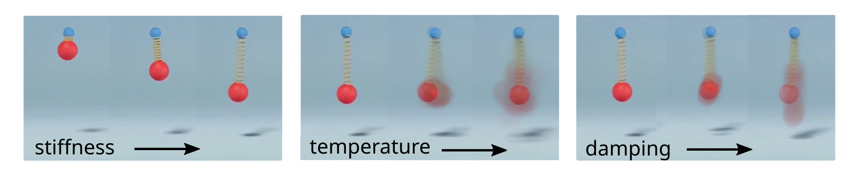
Figure 3: Bead-Spring Mechanics: Inertial Ornstein-Uhlenbeck Process. We consider the stochastic dynamics of the three dimensional I-OU process under different physical conditions including when (i) stiffness decreases (left), (ii) temperature increases (middle), or (iii) damping decreases (right).

The data-driven task is to learn a generative stochastic model $G(\cdot;\theta_{G})$ from observations of trajectories of the system configurations $\mathbf{X}_{[0,\mathcal{T}]}=\{\mathbf{X}(t)\}_{t\in[0,\mathcal{T}]}$, so that $G(\mathbf{Z};\theta_{G})\sim\mathbf{X}_{[0,\mathcal{T}]}$. The $\mathbf{Z}$ is the noise source, here taken to be a high dimensional vector-valued Gaussian with i.i.d components. The $\mathbf{V}(t)$ is not observed directly. We show samples of the training data in Figure 4. Training uses discretized trajectories and trajectory fragments of the form $(\mathbf{X}(t_{1}),\ldots,\mathbf{X}(t_{m}))$. Without using further structure of the data, this task can be challenging given the high dimensional distribution of trajectories $\mathbf{X}(t)$.

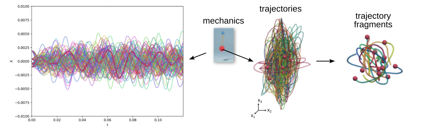
Figure 4: Trajectory Training Data: Inertial Ornstein-Uhlenbeck Process. We show samples of the trajectory data used for training models. The z-component of the trajectory data is shown on the (left). The bead-spring system and traces of the trajectory in three-dimensional space is shown in the (middle). The fragments of the trajectory used during the different training protocols discussed in Section 2.2, on the (right).

The SDYN-GANs uses the probabilistic dependence within the trajectories and the adversarial learning approaches discussed in Section 2.2. This provides flexible methods for learning general models for a wide variety of tasks, even when the generative models may not have readily expressible probability distributions. By using MMD within our SDYN-GANs methods allows for further inductive biases to be introduced based on the type of kernel employed. This can be used to emphasize key features of the empirical distributions being compared. For the OU process studies, we use a RKHS with Rational-Quadratic Kernel (RQK) (Rasmussen and Williams, 2006; Duvenaud, 2014) given by $k(x,y)=\left(1+\frac{\|x-y\|^{2}}{2\alpha\ell^{2}}\right)^{-\alpha}.$ The $\alpha$ determines the rate of decay and $\ell$ provides a characteristic scale for comparisons. The RQK is a characteristic kernel allowing for general comparison of probability distributions (Sriperumbudur et al., 2010). It has the advantage for gradient-based learning of not having an exponentially decaying tail yielding better behaviors in high dimensions (Rasmussen and Williams, 2006; Duvenaud, 2014).

We show a typical training behavior for learning simultaneously parameters $\theta=(K_{0},\gamma,k_{B}T)$ in Figure 5. We find that training initially proceeds by increasing $k_{B}T$ which broadens the generative model distribution to overlap the training data samples to reduce the loss. However, we see that once the stiffness $K_{0}$ and damping $\gamma$ parameters approach reasonable values, around the epoch $\sim 750$, the temperature $k_{B}T$ rapidly decreases to yield models that can more accurately capture the remaining features of the observation data. We see for this training trial that all parameters are close to the correct values around epoch $\sim 1,200$, see Figure 5.

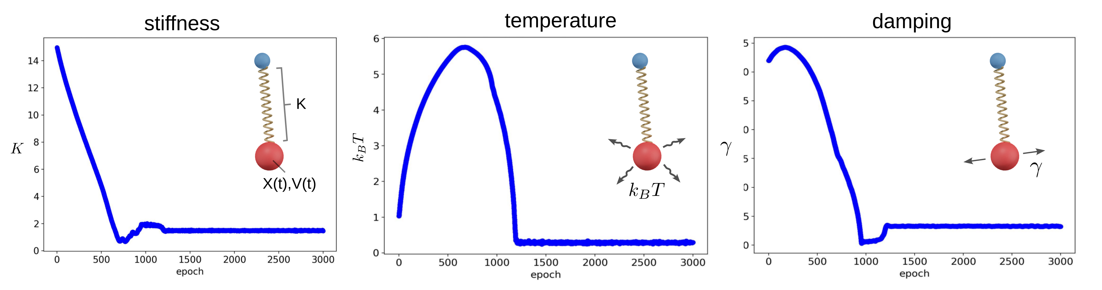
Figure 5: Inertial Ornstein-Uhlenbeck Process: Learning the Stochastic Dynamics. We use SDYN-GANs to learn generative models for the observed trajectories of the stochastic dynamics. We learn simultaneously the drift and diffusive contributions to the dynamics. The target values for this trial were $K_{0}=1.5$, $\gamma=3.2$ and $k_{B}{T}=0.1$. We see early in training the stochastic parameters become large to minimize the loss by enhancing the overlap of the samples of the candidate generative model with the observed samples. As the stiffness and damping parameters become more accurate during training, the stochastic parameters decrease toward the target values.

To investigate further the performance of SDYN-GANs, we perform training using a few different approaches. This includes varying the time-scale $\tau$ overwhich we sample the system configurations $\mathbf{X}(t)$ and the type of distributions implicitly probed. For instance, we use the full-trajectory over a time-duration $\mathcal{T}$, while considering conditionals or marginals statistics over shorter time durations. For this purpose, we use the different training protocols and time-scales $\tau$ discussed in Section 2.2. Throughout, we use the default target model parameters $m=0.1,K_{0}=1.5,\gamma=3.2,k_{B}T=0.1$ and kernel parameters $\alpha=2,\ell=0.01$. For the different SDYN-GANs methods and training protocols, we show the accuracy of our learned generative models in the Tables 1–3.

We find the stiffness and damping mechanics each can be learned with an accuracy of around $5\%$ or less. The thermal fluctuations of the system were more challenging to learn from the trajectory observations. This appeared to arise from other contributing factors to perceived fluctuations associated with sampling errors and a tendency to over-estimate the thermal parameters to help enhance alignment of the candidate generative model with the trajectory data. We found accuracies of only around $50\%$ for the thermal fluctuations of the system. We found the time delay $\tau$ used in probing the temporal sub-sampling of the dynamics can play a significant role in the performance of the learning methods.

Accuracy $K_{0}$ vs $\tau$-Delay
$\tau$-Delay	1.70e-02	1.19e-02	5.83e-03
MMD-full-traj	$1.03e\text{-}02\pm 1.1e\text{-}02$	$2.62e\text{-}02\pm 2.4e\text{-}02$	$1.13e\text{-}02\pm 7.8e\text{-}03$
MMD-conditionals	$9.19e\text{-}03\pm 1.9e\text{-}03$	$2.22e\text{-}02\pm 1.7e\text{-}02$	$2.66e\text{-}02\pm 4.5e\text{-}02$
MMD-marginals	$1.54e\text{-}02\pm 6.7e\text{-}03$	$8.92e\text{-}03\pm 1.1e\text{-}02$	$4.37e\text{-}02\pm 4.5e\text{-}02$
$\tau$-Delay	4.08e-03	2.86e-03	2.00e-03
MMD-full-traj	$1.62e\text{-}02\pm 1.5e\text{-}02$	$8.02e\text{-}03\pm 5.2e\text{-}03$	$1.37e\text{-}02\pm 7.0e\text{-}03$
MMD-conditionals	$1.03e\text{-}01\pm 1.9e\text{-}01$	$8.52e\text{-}01\pm 1.7e\text{+}00$	$5.68e\text{-}01\pm 1.1e\text{+}00$
MMD-marginals	$4.44e\text{-}02\pm 8.0e\text{-}02$	$1.63e\text{+}00\pm 3.2e\text{+}00$	$1.72e\text{+}00\pm 3.4e\text{+}00$

Table 1: Accuracy $K_{0}$ verses $\tau$-Delay: Inertial Ornstein-Uhlenbeck Process. SDYN-GANs training performed using the protocols over the (i) full trajectory, (ii) marginals, and (iii) conditionals, as discussed in Section 2.2. The accuracy of the stiffness estimate $\tilde{\phi}$ for $\phi=K_{0}$ given by the relative error $\epsilon_{\mbox{\tiny rel}}=|\tilde{\phi}-\phi|/|\phi|$. The number of epochs was $3000$. Standard deviations are reported for $4$ runs. The total duration of all trajectories are $t_{n}=1.8\times 10^{-2}$ over $n=18$ steps with $\Delta{t}=10^{-3}$.

For the temporal sampling, we found when the $\tau$ time-scales are relatively large the models were learned more accurately. This appears to be related to the samples better probing the time-scales in the trajectory data overwhich the stiffness and damping make stronger contributions. The longer trajectory durations appear to provide a better signal for learning these properties. As $\tau$ became smaller, we found the accuracy of the learned models decreased for this task.

We further found the training protocol chosen could have a significant impact on the accuracy of the learned models. For the current task, we found throughout that either the full-trajectory protocols or marginals protocols tended to perform the best. A notable feature of the marginals protocol is that the trajectory samples include the same fragments of the trajectory arising in the conditionals, particularly those starting near the sampled initial conditions. This appears to have contributed to the marginals out-performing the conditionals, the latter of which contain less information about the longer-time dynamics.

Accuracy $k_{B}{T}$ vs $\tau$-Delay
$\tau$-Delay	1.70e-02	1.19e-02	5.83e-03
MMD-full-traj	$5.36e\text{-}01\pm 9.5e\text{-}01$	$1.71e\text{+}00\pm 3.4e\text{+}00$	$3.62e\text{+}00\pm 7.1e\text{+}00$
MMD-conditionals	$6.43e\text{-}01\pm 1.1e\text{+}00$	$1.46e\text{+}00\pm 2.6e\text{+}00$	$1.92e\text{+}01\pm 3.8e\text{+}01$
MMD-marginals	$6.54e\text{-}01\pm 1.2e\text{+}00$	$1.51e\text{+}00\pm 2.9e\text{+}00$	$1.39e\text{+}01\pm 2.7e\text{+}01$
$\tau$-Delay	4.08e-03	2.86e-03	2.00e-03
MMD-full-traj	$3.47e\text{+}00\pm 6.7e\text{+}00$	$6.43e\text{+}00\pm 1.3e\text{+}01$	$6.90e\text{+}00\pm 1.4e\text{+}01$
MMD-conditionals	$2.42e\text{+}01\pm 4.7e\text{+}01$	$9.54e\text{+}01\pm 1.7e\text{+}02$	$9.38e\text{+}01\pm 1.7e\text{+}02$
MMD-marginals	$1.85e\text{+}01\pm 3.7e\text{+}01$	$3.95e\text{+}01\pm 7.9e\text{+}01$	$3.82e\text{+}01\pm 7.6e\text{+}01$

Table 2: Accuracy $k_{B}{T}$ verses $\tau$-Delay: Inertial Ornstein-Uhlenbeck Process. SDYN-GANs training performed using the protocols over the (i) full trajectory, (ii) marginals, and (iii) conditionals, as discussed in Section 2.2. The accuracy of the temperature estimate $\tilde{\phi}$ for $\phi=k_{B}{T}$ given by the relative error $\epsilon_{\mbox{\tiny rel}}=|\tilde{\phi}-\phi|/|\phi|$. The number of epochs was $3000$. Standard deviations are reported for $4$ runs. The total duration of all trajectories are $t_{n}=1.8\times 10^{-2}$ over $n=18$ steps with $\Delta{t}=10^{-3}$.

We found overall a better job was done by the full-trajectory training protocol which uses more steps along the trajectory than the marginals and conditionals protocols. The marginals also tended to do better than the conditionals. As an exception, we did find in a few cases for small $\tau$ the conditionals did a better job than the marginals in estimating the stiffness. This was perhaps since when working over shorter time durations, the more temporally localized sampling near the same initial conditions in the conditionals provide more consistent and less obscured information on the stiffness responses, relative to the full set of trajectory fragments contributing in the marginals protocols.

Accuracy $\gamma$ vs $\tau$-Delay
$\tau$-Delay	1.70e-02	1.19e-02	5.83e-03
MMD-full-traj	$1.53e\text{-}02\pm 1.5e\text{-}02$	$3.31e\text{-}02\pm 2.5e\text{-}02$	$2.91e\text{-}02\pm 4.3e\text{-}02$
MMD-conditionals	$2.85e\text{-}02\pm 2.3e\text{-}02$	$6.57e\text{-}02\pm 6.0e\text{-}02$	$2.29e\text{-}02\pm 3.3e\text{-}02$
MMD-marginals	$1.67e\text{-}02\pm 8.4e\text{-}03$	$3.34e\text{-}02\pm 1.9e\text{-}02$	$6.20e\text{-}02\pm 8.9e\text{-}02$
$\tau$-Delay	4.08e-03	2.86e-03	2.00e-03
MMD-full-traj	$5.20e\text{-}02\pm 4.7e\text{-}02$	$4.70e\text{-}02\pm 4.6e\text{-}02$	$2.20e\text{-}02\pm 1.8e\text{-}02$
MMD-conditionals	$2.00e\text{-}01\pm 3.7e\text{-}01$	$1.91e\text{+}00\pm 3.8e\text{+}00$	$1.88e\text{+}00\pm 3.7e\text{+}00$
MMD-marginals	$1.90e\text{-}01\pm 3.0e\text{-}01$	$5.54e\text{+}00\pm 1.1e\text{+}01$	$5.47e\text{+}00\pm 1.1e\text{+}01$

Table 3: Accuracy $\gamma$ verses $\tau$-Delay: Inertial Ornstein-Uhlenbeck Process. SDYN-GANs training performed using the protocols over the (i) full trajectory, (ii) marginals, and (iii) conditionals, as discussed in Section 2.2. The accuracy of the damping estimate $\tilde{\phi}$ for $\phi=\gamma$ given by the relative error $\epsilon_{\mbox{\tiny rel}}=|\tilde{\phi}-\phi|/|\phi|$. The number of epochs was $3000$. Standard deviations are reported for $4$ runs. The total duration of all trajectories are $t_{n}=1.8\times 10^{-2}$ over $n=18$ steps with $\Delta{t}=10^{-3}$.

For the longer $\tau$ cases when comparing with the conditionals, the marginals tended to more accurately estimate simultaneously the stiffness and damping. This likely arose, since unlike the conditionals case, the marginals do not require the initial parts of the trajectory fragments being compared to share the same initial conditions. For the general short-duration fragments, there is additional information on the long-time dynamical responses contributing to the marginals. In summary, the results suggest using the full-trajectory protocols when possible and relatively long $\tau$ sampling. When one is only able to probe short-duration trajectory fragments, the results suggest the marginals provide some advantages over the conditionals. Which protocols work best may be dependent on the task and the time-scales associated with the dynamical behaviors being modeled. These results show a few strategies for using SDYN-GANs to learn generative models for stochastic systems.

5.3 Learning Unknown Force-Laws with SDYN-GANs Generative Modeling

We show how SDYN-GANs can be used to learn force-laws $\mathbf{F}(\mathbf{X})$ from observations of trajectories of stochastic systems. We consider the inertial Langevin dynamics of particle systems of the form

$$md\mathbf{V}(t)=-\gamma\mathbf{V}(t)dt+\mathbf{F}(\mathbf{X};\theta_{F})dt+\sqrt{2k_{B}{T}\gamma}d\mathbf{W}(t),\;\;\;d\mathbf{X}(t)=\mathbf{V}(t)dt,$$ (17)

where $\mathbf{X},\mathbf{V}\in\mathbb{R}^{3}$. The force-law $\mathbf{F}(\mathbf{X})$ will be modeled using Deep Neural Networks (DNNs) (LeCun et al., 2015; Goodfellow et al., 2016). In this case, $\theta_{F}$ are the DNN weights and biases to be learned. We consider here the case of radial potentials $\mathbf{F}(\mathbf{X})=\mathbf{F}(\|\mathbf{X}\|)=F(r)\mathbf{e}_{r}$ with $\mathbf{e}_{r}=\mathbf{X}/\|\mathbf{X}\|$. For simplicity, we focus on the case where $m,\gamma,T$ are fixed, but these also could be learned in conjunction with the force-law. The data-driven task is to learn DNN representations $\mathbf{F}(\mathbf{X};\theta_{F})$ for the force-law from the configuration trajectories $\mathbf{X}_{[0,\mathcal{T}]}=\{\mathbf{X}(t)\}_{t\in[0,\mathcal{T}]}$ discretized as $(\mathbf{X}(t_{1}),\ldots,\mathbf{X}(t_{n}))$, see Figure 6. The $\mathbf{V}(t)$ is not observed directly. We use for our generative models the Langevin dynamics of equation 17 approximated by the $(m=2)$-step stochastic numerical discretizations discussed in Section 5.1. We show samples of the training data in Figure 7.

Figure 6: Learning Unknown Force-Laws. SDYN-GANs is used to learn an unknown force-law from observation of particle trajectories (left). The learned force-law can be represented using neural networks or other model classes (middle). The generative models use the dependence in the probabilities of the stochastic trajectories using $m$-step stochastic numerical discretizations (right). The models are learned using a few different training protocols using statistics of the (i) full-trajectory, (ii) conditionals, and (iii) marginals, as discussed in Section 2.2.

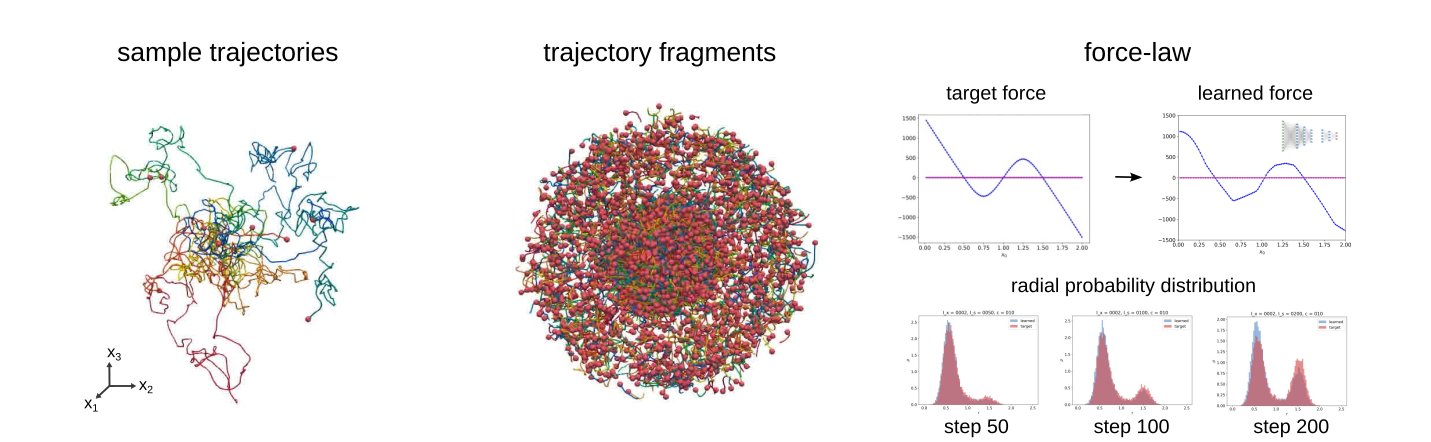
Figure 7: Learning Unknown Force Laws: Trajectory Data. We show a few samples of the particle trajectories (left). The force-law is learned from samples of trajectory fragments using the different training protocols discussed in Section 2.2, (middle). SDYN-GANs is used to learn a neural network representation of the force-law from observations of trajectories of the particle system. We evaluate the final accuracy of the learned model by considering the relative $L^{1}$-norm of the marginal time-dependent radial probability distributions of samples of the learned model compared with the target particle system (right).

In our generative models, we use DNN architectures of multi-layer perceptrons with input-hidden-output sizes $n_{\mbox{\tiny in}}{{\mbox{-}}}n_{1}{{\mbox{-}}}n_{2}{{\mbox{-}}}n_{3}{{\mbox{-}}}n_{\mbox{\tiny out}}$ and LeakyReLU (Xu et al., 2015) units with slope=-0.01. In the DNNs we use $n_{\mbox{\tiny out}}=n_{\mbox{\tiny in}}=1$, with default values of $n_{1}=n_{2}=n_{3}=100$ and biases for all layers except for the last layer. The DNNs serve to model the $F$ in the radial force $\mathbf{F}=F(r;\theta_{F})\mathbf{e}_{r}$.

We use SDYN-GANs to learn generative models by probing trajectories on different time-scales $\tau$ and training protocols that are based on sampling the (i) full-trajectory, (ii) conditionals, and (iii) marginals, as discussed in Section 2.2. To train the models, we simulate the trajectories of the candidate generative models and compare with the samples of the observation training data. To characterize the final accuracy of the learned models, we use the relative errors under the $L^{1}$-norm of the time-dependent radial probability distributions to compare the samples of the generative model with the target particle system. We emphasize the $L^{1}$-error is not used during training, but only on the final models to characterize the accuracy of the stochastic trajectories they generate. We train using SDYN-GANs with different time-scales $\tau$ and training protocols, with our results reported in Table 4.

Accuracy vs $\tau$-Delay
Method / $\mathbf{\tau}$-Delay	1.90e-02	1.16e-02	7.12e-03
MMD-full-traj ($I_{s}=50$)	$1.20e\text{-}01\pm 4.9e\text{-}02$	$1.02e\text{-}01\pm 4.1e\text{-}02$	$8.67e\text{-}02\pm 3.2e\text{-}02$
MMD-conditionals	$1.33e\text{-}01\pm 3.5e\text{-}02$	$1.42e\text{-}01\pm 6.1e\text{-}02$	$1.42e\text{-}01\pm 4.2e\text{-}02$
MMD-marginals	$8.20e\text{-}02\pm 4.5e\text{-}02$	$1.05e\text{-}01\pm 3.4e\text{-}02$	$9.00e\text{-}02\pm 2.3e\text{-}02$
MMD-full-traj ($I_{s}=100$)	$1.56e\text{-}01\pm 8.8e\text{-}02$	$1.27e\text{-}01\pm 4.3e\text{-}02$	$1.06e\text{-}01\pm 2.8e\text{-}02$
MMD-conditionals	$1.39e\text{-}01\pm 4.0e\text{-}02$	$1.68e\text{-}01\pm 5.7e\text{-}02$	$1.33e\text{-}01\pm 4.7e\text{-}02$
MMD-marginals	$9.75e\text{-}02\pm 4.7e\text{-}02$	$9.96e\text{-}02\pm 3.4e\text{-}02$	$9.97e\text{-}02\pm 2.3e\text{-}02$
MMD-full-traj ($I_{s}=200$)	$2.22e\text{-}01\pm 1.6e\text{-}01$	$1.69e\text{-}01\pm 7.7e\text{-}02$	$1.51e\text{-}01\pm 3.8e\text{-}02$
MMD-conditionals	$1.67e\text{-}01\pm 6.2e\text{-}02$	$2.28e\text{-}01\pm 8.3e\text{-}02$	$2.28e\text{-}01\pm 3.7e\text{-}02$
MMD-marginals	$1.16e\text{-}01\pm 3.1e\text{-}02$	$1.24e\text{-}01\pm 2.3e\text{-}02$	$1.15e\text{-}01\pm 2.4e\text{-}02$

Table 4: $L^{1}$-Accuracy of Learned Force-Law. We investigate how the relative $L^{1}$-errors of the time-dependent marginal probability densities at times $I_{step}=50,100,200$, $\mbox{epoch}=5000$, compare between the learned generative models and the target stochastic process. The mean and standard deviation are reported over 5 runs. SDYN-GANs training protocols are based on trajectory samples from distributions of the (i) full trajectory, (ii) conditionals, and (iii) marginals, for details see Section 2.2. The $L^{1}$-relative-errors of the empirical radial probability distributions were computed from histograms using the range $[0,L]$ with $L=2.5$ and bin-width $\Delta{x}=0.05$. The total duration of all trajectories are $t_{n_{t}}=2.0\times 10^{-2}$ over $n_{t}=20$ steps with $\Delta{t}=10^{-3}$.

We find the generative models learn the force-law with an accuracy of around $20\%$. We found the training protocols using the full trajectory and the marginals performed best, see Table 4. We remark that in theory the large $\tau$ in the infinite time horizon limit would give samples for $\mathbf{X}$ from the equilibrium Gibbs-Boltzmann distribution, $\rho(\mathbf{X})=1/Z\exp\left(-U(\mathbf{X})/k_{B}{T}\right)$. The equilibrium distribution only depends on the potential $U$ of the force-law. Interestingly, we find in the training there was not a strong dependence in the results on the choice of $\tau$. The results highlight that in contrast to equilibrium estimators, the SDYN-GANs learning methods allow for flexibility in estimating the force-law even in the non-equilibrium setting and from observations over shorter-time trajectories relative to the equilibration time-scale.

We found for this task the sampling from the full trajectory and marginals tended to perform better than the conditionals. For the shorter-time durations, this appears to arise from the marginals including contributions from trajectory fragments that are included in the conditionals and also trajectory fragments from later parts of the trajectories. Again, this provides additional information on the longer-time dynamical responses, here enhancing learning of the force-laws. The matching of the marginals also may be more stringent during training than the conditionals. Obtaining agreement requires more global coordination in the generated trajectories so that statistics of later segments of the trajectory match the observed target system.

We remark that for both the conditionals and marginals, the use of shorter duration trajectory fragments helps reduce the dimensionality of the samples. This appears to improve in the loss function the ability to make comparisons with the observation data. The results indicate the marginals again may provide some advantages for training SDYN-GANs when one is able only to probe trajectory data in fragments over relatively short time durations.

In summary, the results show a few strategies for using SDYN-GANs for learning non-linear force-laws and other physical properties from observations of the system dynamics. The samples-based methods of SDYN-GANs allows for general generative modeling classes to be used, without a need for specification of likelihood functions. This facilitates the use of general generative models for learning representations of stochastic systems. The SDYN-GANs approaches also can be used for non-neural network modeling classes, and combined with other training protocols, such as data augmentation, further regularizations, and other prior information motivated by the task and knowledge from the application domain.

6 Conclusions

We introduced SDYN-GANs for adversarial learning of generative models for representing stochastic dynamical systems. A key feature of our approaches is that they require only empirical trajectory samples from the candidate generative model for comparison with observation data. This allows for using a wide class of generative models without the need for specifying likelihood functions. We also developed a class of generative models based on stable $m$-step stochastic numerical integrators facilitating learning models for long-time predictions and simulations. We introduced several training methods for probing dynamics on different time-scales, utilizing probabilistic dependencies, and for leveraging different statistical properties of the conditional and marginal distributions. As discussed in our results, this provides strategies to reduce the dimensionality of the statistics used during training. This also provides flexibility in how features of the dynamics are used in learning the generative models. Our developed SDYN-GANs approaches facilitate learning robust stochastic dynamical models which can be used in diverse tasks arising in machine learning, statistical inference, dynamical systems identification, and scientific computation.

Appendix

Appendix A Gradient Equations for $m$-Step Generative Models

For our $m$-step generative models, the use of direct backpropagation for book-keeping the forward calculations in generating trajectory samples can result in prohibitively large computational call graphs. This is further increased as the time duration of the trajectories grow. We derive alternative adjoint approaches to obtain more efficient methods for loss functions to compute the gradients needed during training.

For our general $m$-step generative models discussed in Section 4.2, we use the formulation $\mathbf{f}(\mathbf{x},\mathbf{p})=0$. For $m\leq j\leq N$, we have

$$[\mathbf{f}]_{(j,d)}=\left[\mathbf{X}_{j}-\boldsymbol{\Psi}_{j-1}(\mathbf{X}_{j-1},\ldots,\mathbf{X}_{j-m},\boldsymbol{\omega}_{j-1};\mathbf{p})\right]^{(d)}=0.$$ (18)

The index $(j,d)$ refers to the $j^{th}$ time-step and $d^{th}$ dimension component associated with $\mathbf{X}_{j}^{(d)}$. We use for this the notations $\mathbf{X}_{j}^{(d)}=\left[\mathbf{X}_{j}\right]^{(d)}=\mathbf{X}_{(j,d)}$. The update map is denoted as $\boldsymbol{\Psi}_{j-1}$. For $j=0,\ldots,m-1$, we have

$$[\mathbf{f}]_{(0,d)}=\left[\mathbf{X}_{0}-\mathbf{x}_{0}\right]^{(d)}=0,\;\;[\mathbf{f}]_{(m-1,d)}=\left[\mathbf{X}_{m-1}-\mathbf{x}_{m-1}\right]^{(d)}=0.$$ (19)

We can then provide the gradients for $\nabla_{X_{k}}\boldsymbol{\Psi}_{k},\ldots,\nabla_{X_{k}}\boldsymbol{\Psi}_{k+m}$ and other terms.

We derive methods for solving efficiently $J^{T}\mathbf{r}=-\mathbf{f}_{p}$ for $\mathbf{r}$ where $J=\mathbf{f}_{x}$. For details motivating this formulation, see Section 4.2. By using the structure of $J=\mathbf{f}_{x}$ from equations 18– 19, we can obtain the following set of recurrence equations for the components of $\mathbf{r}$. For $0\leq k\leq N-m$, we have

$$r_{(j,d)}f_{(j,d),(k,d^{\prime})}=r_{(k,d)}\delta_{d,d^{\prime}}-\left[\nabla_{X_{(k,d^{\prime})}}\Psi_{(k,d)}\right]r_{(k+1,d)}\cdots-\left[\nabla_{X_{(k,d^{\prime})}}\Psi_{(k+m,d)}\right]r_{{(k+m,d)}}=\frac{\partial\phi}{\partial X_{(k,d^{\prime})}}.$$ (20)

For $k=N-\ell,\;1\leq\ell\leq m-1$, we have

$$r_{(j,d)}f_{(j,d),(k,d^{\prime})}=r_{(k,d)}\delta_{d,d^{\prime}}-\left[\nabla_{X_{(k,d^{\prime})}}\Psi_{(k,d)}\right]r_{(k+1,d)}\cdots-\left[\nabla_{X_{(k,d^{\prime})}}\Psi_{(k+\ell,d)}\right]r_{{(k+\ell,d)}}=\frac{\partial\phi}{\partial X_{(k,d^{\prime})}}.$$ (21)

For $k=N$, we have

$$r_{(j,d)}f_{(j,d),(k,d^{\prime})}=r_{(N,d)}\delta_{d,d^{\prime}}=\frac{\partial\phi}{\partial X_{(N,d^{\prime})}}.$$ (22)

This gives an $m^{th}$-order recurrence relation we can use to propagate values from $N,N-1,\ldots,0$ to obtain the components of $\mathbf{r}$.

To obtain $\mathbf{f}_{p}$, we have for $m\leq j\leq N$, that

$$[\mathbf{f}_{p}]_{(j,d)}=-\nabla_{p}\boldsymbol{\Psi}_{(j-1,d)}.$$ (23)

For $0\leq j\leq m-1$, we have

$$[\mathbf{f}]_{(j,d)}=\left[\mathbf{X}_{j}-\mathbf{x}_{j}\right]^{(d)}=0,\;\;[\mathbf{f}]_{(j,d),(k,d^{\prime})}=\delta_{(j,d),(k,d^{\prime})},\;\;[\mathbf{f}_{p}]_{(j,d)}=-\frac{\partial\left[\mathbf{x}_{j}\right]^{(d)}}{\partial p}.$$ (24)

We compute the gradients needed for training by using

$$\nabla_{p}\tilde{g}=\tilde{\mathbf{g}}_{p}-\mathbf{r}^{T}\mathbf{f}_{p}.$$ (25)

To compute $\mathbf{r}$, we solve for each sample $\mathbf{X}^{[i]}$ of the stochastic trajectories the $m^{th}$-order recurrence relations given in equations 20– 22. The $\tilde{\mathbf{g}}_{p}=\partial\tilde{\mathbf{g}}/\partial p$ and $\mathbf{f}_{p}$ are computed using equations 23– 24. The final gradient is computed by averaging using $\nabla_{p}\bar{g}=\frac{1}{M}\sum_{1=1}^{M}\nabla_{p}\tilde{g}^{[i]}$ over the $M$ samples of the stochastic trajectories indexed by $[i]$. There are also ways to obtain additional efficiencies by using structure of the specific loss functions, as we discuss in Section 4.3. We use equations 18– 25 to develop efficient methods for computing the gradients of our $m$-step generative models.

References

- Abbati et al. (2019) Gabriele Abbati, Philippe Wenk, Michael A. Osborne, Andreas Krause, Bernhard Schölkopf, and Stefan Bauer. AReS and MaRS adversarial and MMD-minimizing regression for SDEs. In Kamalika Chaudhuri and Ruslan Salakhutdinov, editors, Proceedings of the 36th International Conference on Machine Learning, volume 97 of Proceedings of Machine Learning Research, pages 1–10. PMLR, 09–15 Jun 2019. URL https://proceedings.mlr.press/v97/abbati19a.html.
- Aït-Sahalia and Kimmel (2007) Yacine Aït-Sahalia and Robert Kimmel. Maximum likelihood estimation of stochastic volatility models. Journal of financial economics, 83(2):413–452, 2007.
- Arjovsky et al. (2017) Martin Arjovsky, Soumith Chintala, and Léon Bottou. Wasserstein generative adversarial networks. In Doina Precup and Yee Whye Teh, editors, Proceedings of Machine Learning Research, volume 70 of Proceedings of Machine Learning Research, pages 214–223, International Convention Centre, Sydney, Australia, 06–11 Aug 2017. PMLR. URL http://proceedings.mlr.press/v70/arjovsky17a.html.
- Aronszajn (1950) N. Aronszajn. Theory of reproducing kernels. Transactions of the American Mathematical Society, 68(3):337–404, 1950. ISSN 00029947. URL http://www.jstor.org/stable/1990404.
- Atzberger et al. (2007) Paul J Atzberger, Peter R Kramer, and Charles S Peskin. A stochastic immersed boundary method for fluid-structure dynamics at microscopic length scales. Journal of Computational Physics, 224(2):1255–1292, 2007.
- Berlinet and Thomas-Agnan (2011) Alain Berlinet and Christine Thomas-Agnan. Reproducing kernel Hilbert spaces in probability and statistics. Springer Science & Business Media, 2011.
- Binkowski et al. (2018) Mikołaj Binkowski, Dougal J. Sutherland, Michael Arbel, and Arthur Gretton. Demystifying MMD GANs. In International Conference on Learning Representations, 2018. URL https://openreview.net/forum?id=r1lUOzWCW.
- Bishop (2006) Christopher M. Bishop. Pattern Recognition and Machine Learning (Information Science and Statistics). Springer-Verlag, Berlin, Heidelberg, 2006. ISBN 0387310738.
- Bottou et al. (1991) Léon Bottou et al. Stochastic gradient learning in neural networks. Proceedings of Neuro-Nımes, 91(8):12, 1991.
- Buckwar and Winkler (2006) Evelyn Buckwar and Renate Winkler. Multistep methods for sdes and their application to problems with small noise. SIAM journal on numerical analysis, 44(2):779–803, 2006.
- Burden and Faires (2010) Richard L. Burden and Douglas Faires. Numerical Analysis. Brooks/Cole Cengage Learning, 2010.
- Céa (1986) Jean Céa. Conception optimale ou identification de formes, calcul rapide de la dérivée directionnelle de la fonction coût. ESAIM: Mathematical Modelling and Numerical Analysis-Modélisation Mathématique et Analyse Numérique, 20(3):371–402, 1986.
- Chen et al. (2018) Tian Qi Chen, Yulia Rubanova, Jesse Bettencourt, and David Duvenaud. Neural ordinary differential equations. In Samy Bengio, Hanna M. Wallach, Hugo Larochelle, Kristen Grauman, Nicolò Cesa-Bianchi, and Roman Garnett, editors, Advances in Neural Information Processing Systems 31: Annual Conference on Neural Information Processing Systems 2018, NeurIPS 2018, 3-8 December 2018, Montréal, Canada, pages 6572–6583, 2018. URL http://papers.nips.cc/paper/7892-neural-ordinary-differential-equations.
- Cover and Thomas (2006) Thomas M. Cover and Joy A. Thomas. Elements of Information Theory (Wiley Series in Telecommunications and Signal Processing). Wiley-Interscience, USA, 2006. ISBN 0471241954.
- Cramer (1989) Jan Salomon Cramer. Econometric applications of maximum likelihood methods. CUP Archive, 1989.
- de Avila Belbute-Peres et al. (2018) Filipe de Avila Belbute-Peres, Kevin Smith, Kelsey Allen, Josh Tenenbaum, and J Zico Kolter. End-to-end differentiable physics for learning and control. Advances in neural information processing systems, 31, 2018.
- Deshpande et al. (2019) Ishan Deshpande, Yuan-Ting Hu, Ruoyu Sun, Ayis Pyrros, Nasir Siddiqui, Sanmi Koyejo, Zhizhen Zhao, David Forsyth, and Alexander G. Schwing. Max-sliced wasserstein distance and its use for gans, 2019.
- Ding et al. (2020) Mucong Ding, Constantinos Daskalakis, and Soheil Feizi. Subadditivity of probability divergences on bayes-nets with applications to time series gans. preprint arxiv:2003.00652, 2020. URL https://arxiv.org/abs/2003.00652.
- Ding et al. (2021) Mucong Ding, Constantinos Daskalakis, and Soheil Feizi. Gans with conditional independence graphs: On subadditivity of probability divergences. In Arindam Banerjee and Kenji Fukumizu, editors, Proceedings of The 24th International Conference on Artificial Intelligence and Statistics, volume 130 of Proceedings of Machine Learning Research, pages 3709–3717. PMLR, 13–15 Apr 2021. URL https://proceedings.mlr.press/v130/ding21e.html.
- Dudko et al. (2002) OK Dudko, AE Filippov, J Klafter, and M Urbakh. Dynamic force spectroscopy: a fokker–planck approach. Chemical Physics Letters, 352(5-6):499–504, 2002.
- Duvenaud (2014) David Duvenaud. The kernel cookbook: Advice on covariance functions. URL https://www. cs. toronto. edu/~ duvenaud/cookbook, 2014.
- Dziugaite et al. (2015) Gintare Karolina Dziugaite, Daniel M. Roy, and Zoubin Ghahramani. Training generative neural networks via maximum mean discrepancy optimization. In Proceedings of the Thirty-First Conference on Uncertainty in Artificial Intelligence, UAI’15, page 258–267, Arlington, Virginia, USA, 2015. AUAI Press. ISBN 9780996643108. URL https://arxiv.org/abs/1505.03906.
- Ewald and Témam (2005) Brian D Ewald and Roger Témam. Numerical analysis of stochastic schemes in geophysics. SIAM journal on numerical analysis, 42(6):2257–2276, 2005.
- Fisher and Russell (1922) R. A. Fisher and Edward John Russell. On the mathematical foundations of theoretical statistics. Philosophical Transactions of the Royal Society of London. Series A, Containing Papers of a Mathematical or Physical Character, 222(594-604):309–368, 1922. doi: 10.1098/rsta.1922.0009. URL https://royalsocietypublishing.org/doi/abs/10.1098/rsta.1922.0009.
- Fortet and Mourier (1953) Robert Fortet and Edith Mourier. Convergence de la répartition empirique vers la répartition théorique. Annales scientifiques de l’École Normale Supérieure, 3e série, 70(3):267–285, 1953. doi: 10.24033/asens.1013. URL http://www.numdam.org/articles/10.24033/asens.1013/.
- Frenkel and Smit (2001) Daan Frenkel and Berend Smit. Understanding molecular simulation: from algorithms to applications, volume 1. Elsevier, 2001.
- Gardiner (1985) C. W. Gardiner. Handbook of stochastic methods. Series in Synergetics. Springer, 1985.
- Gelman et al. (1995) Andrew Gelman, John B Carlin, Hal S Stern, and Donald B Rubin. Bayesian data analysis. Chapman and Hall/CRC, 1995.
- Giles and Glasserman (2006) Michael Giles and Paul Glasserman. Smoking adjoints: fast evaluation of greeks in monte carlo calculations. Risk, 2006. URL http://citeseerx.ist.psu.edu/viewdoc/summary?doi=10.1.1.132.2360.
- Giles and Pierce (2000) Michael B. Giles and Niles A. Pierce. An introduction to the adjoint approach to design. Flow, Turbulence and Combustion, 65(3):393–415, 2000. ISSN 1573-1987. doi: 10.1023/A:1011430410075. URL https://doi.org/10.1023/A:1011430410075.
- Giorgini et al. (2020) L. T. Giorgini, W. Moon, and J. S. Wettlaufer. Analytical survival analysis of the ornstein-uhlenbeck process. Journal of Statistical Physics, 181(6):2404–2414, 2020. ISSN 1572-9613. doi: 10.1007/s10955-020-02669-y. URL https://doi.org/10.1007/s10955-020-02669-y.
- Goerlich et al. (2021) Rémi Goerlich, Minghao Li, Samuel Albert, Giovanni Manfredi, Paul-Antoine Hervieux, and Cyriaque Genet. Noise and ergodic properties of brownian motion in an optical tweezer: Looking at regime crossovers in an ornstein-uhlenbeck process. Physical Review E, 103(3):032132, 2021.
- Gomez-Solano et al. (2010) J. R. Gomez-Solano, L. Bellon, A. Petrosyan, and S. Ciliberto. Steady-state fluctuation relations for systems driven by an external random force. EPL (Europhysics Letters), 89(6):60003, mar 2010. doi: 10.1209/0295-5075/89/60003. URL https://doi.org/10.1209/0295-5075/89/60003.
- Goodfellow et al. (2014) Ian Goodfellow, Jean Pouget-Abadie, Mehdi Mirza, Bing Xu, David Warde-Farley, Sherjil Ozair, Aaron Courville, and Yoshua Bengio. Generative adversarial nets. In Z. Ghahramani, M. Welling, C. Cortes, N. D. Lawrence, and K. Q. Weinberger, editors, Advances in Neural Information Processing Systems 27, pages 2672–2680. Curran Associates, Inc., 2014. URL http://papers.nips.cc/paper/5423-generative-adversarial-nets.pdf.
- Goodfellow et al. (2016) Ian Goodfellow, Yoshua Bengio, and Aaron Courville. Deep Learning. The MIT Press, 2016. ISBN 0262035618. URL https://www.deeplearningbook.org/.
- Gretton et al. (2012) Arthur Gretton, Karsten M. Borgwardt, Malte J. Rasch, Bernhard Schölkopf, and Alexander Smola. A kernel two-sample test. Journal of Machine Learning Research, 13(25):723–773, 2012. URL http://jmlr.org/papers/v13/gretton12a.html.
- Gronbech-Jensen and Farago (2013) Niels Gronbech-Jensen and Oded Farago. A simple and effective verlet-type algorithm for simulating langevin dynamics. Molecular Physics, 111(8):983–991, Feb 2013. ISSN 1362-3028. doi: 10.1080/00268976.2012.760055. URL http://dx.doi.org/10.1080/00268976.2012.760055.
- Gross et al. (2020) B.J. Gross, N. Trask, P. Kuberry, and P.J. Atzberger. Meshfree methods on manifolds for hydrodynamic flows on curved surfaces: A generalized moving least-squares (gmls) approach. Journal of Computational Physics, 409:109340, 2020. ISSN 0021-9991. doi: 10.1016/j.jcp.2020.109340. URL https://doi.org/10.1016/j.jcp.2020.109340.
- Gulrajani et al. (2017) Ishaan Gulrajani, Faruk Ahmed, Martin Arjovsky, Vincent Dumoulin, and Aaron C Courville. Improved training of wasserstein gans. In I. Guyon, U. V. Luxburg, S. Bengio, H. Wallach, R. Fergus, S. Vishwanathan, and R. Garnett, editors, Advances in Neural Information Processing Systems 30, pages 5767–5777. Curran Associates, Inc., 2017. URL http://papers.nips.cc/paper/7159-improved-training-of-wasserstein-gans.pdf.
- Hald (1999) Anders Hald. On the history of maximum likelihood in relation to inverse probability and least squares. Statistical Science, 14(2):214–222, 1999. ISSN 08834237. URL http://www.jstor.org/stable/2676741.
- Hansen (1982) Lars Peter Hansen. Large sample properties of generalized method of moments estimators. Econometrica: Journal of the econometric society, pages 1029–1054, 1982.
- Hurn et al. (2007) A Stan Hurn, JI Jeisman, and Kenneth A Lindsay. Seeing the wood for the trees: A critical evaluation of methods to estimate the parameters of stochastic differential equations. Journal of Financial Econometrics, 5(3):390–455, 2007.
- Iserles (2009) Arieh Iserles. A first course in the numerical analysis of differential equations. Cambridge university press, 2009.
- Jasuja and Atzberger (2022) Dev Jasuja and P. J. Atzberger. Magnus exponential integrators for stiff time-varying stochastic systems. preprint arxiv 2212.08978, 2022. doi: 10.48550/ARXIV.2212.08978. URL https://arxiv.org/abs/2212.08978.
- Jensen and Poulsen (2002) Bjarke Jensen and Rolf Poulsen. Transition densities of diffusion processes. The Journal of Derivatives, 9(4):18–32, 2002. ISSN 1074-1240. doi: 10.3905/jod.2002.319183. URL https://jod.pm-research.com/content/9/4/18.
- Jittorntrum (1978) K. Jittorntrum. An implicit function theorem. Journal of Optimization Theory and Applications, 25(4):575–577, 1978. ISSN 1573-2878. doi: 10.1007/BF00933522. URL https://doi.org/10.1007/BF00933522.
- Kaebe et al. (2009) C. Kaebe, J. H. Maruhn, and E. W. Sachs. Adjoint-based monte carlo calibration of financial market models. Finance and Stochastics, 13(3):351–379, 2009. ISSN 1432-1122. doi: 10.1007/s00780-009-0097-9. URL https://doi.org/10.1007/s00780-009-0097-9.
- Kalman (1960) R. E. Kalman. A New Approach to Linear Filtering and Prediction Problems. Journal of Basic Engineering, 82(1):35–45, 03 1960. ISSN 0021-9223. doi: 10.1115/1.3662552. URL https://doi.org/10.1115/1.3662552.
- Kidger et al. (2021) Patrick Kidger, James Foster, Xuechen Li, and Terry J Lyons. Neural sdes as infinite-dimensional gans. In International Conference on Machine Learning, pages 5453–5463. PMLR, 2021.
- Kim et al. (1998) Sangjoon Kim, Neil Shephard, and Siddhartha Chib. Stochastic volatility: likelihood inference and comparison with arch models. The review of economic studies, 65(3):361–393, 1998. URL https://doi.org/10.1111/1467-937X.00050.
- King (1998) Gary King. Unifying political methodology: The likelihood theory of statistical inference. University of Michigan Press, 1998.
- Kingma and Ba (2014) Diederik P Kingma and Jimmy Ba. Adam: A method for stochastic optimization. preprint arXiv:1412.6980, 2014. URL https://arxiv.org/abs/1412.6980.
- Kloeden and Platen (1992) P.E. Kloeden and E. Platen. Numerical solution of stochastic differential equations. Springer-Verlag, 1992.
- Kodali et al. (2017) Naveen Kodali, Jacob Abernethy, James Hays, and Zsolt Kira. On convergence and stability of gans. arXiv preprint arXiv:1705.07215, 2017.
- Kullback and Leibler (1951) S. Kullback and R. A. Leibler. On information and sufficiency. Ann. Math. Statist., 22(1):79–86, 03 1951. doi: 10.1214/aoms/1177729694. URL https://doi.org/10.1214/aoms/1177729694.
- Large (2021) Steven J Large. Stochastic control in microscopic nonequilibrium systems. In Dissipation and Control in Microscopic Nonequilibrium Systems, pages 91–111. Springer, 2021.
- LeCun et al. (2015) Yann LeCun, Yoshua Bengio, and Geoffrey Hinton. Deep learning. Nature, 521(7553):436–444, May 2015. ISSN 1476-4687. URL https://doi.org/10.1038/nature14539.
- Li et al. (2015) Yujia Li, Kevin Swersky, and Richard S. Zemel. Generative moment matching networks. In Francis R. Bach and David M. Blei, editors, Proceedings of the 32nd International Conference on Machine Learning, ICML 2015, Lille, France, 6-11 July 2015, volume 37 of JMLR Workshop and Conference Proceedings, pages 1718–1727. JMLR.org, 2015. URL http://proceedings.mlr.press/v37/li15.html.
- Lin (1991) J. Lin. Divergence measures based on the shannon entropy. IEEE Transactions on Information Theory, 37(1):145–151, 1991. doi: 10.1109/18.61115.
- Lions (1971) Jacques Louis Lions. Optimal Control of Systems Governed by Partial Differential Equations. Springer-Verlag, Berlin, 1971.
- Ljung (1987) Lennart Ljung. System Identification. Prentice Hall, 1987. ISBN ISBN 10: 0136566952 ISBN 13: 9780136566953. URL https://www.amazon.com/System-Identification-Theory-User-2nd/dp/0136566952.
- Lopez and Atzberger (2022) Ryan Lopez and Paul J. Atzberger. Gd-vaes: Geometric dynamic variational autoencoders for learning nonlinear dynamics and dimension reductions. preprint arxiv:2206.05183, 2022. URL https://arxiv.org/abs/2206.05183.
- Lydia and Francis (2019) Agnes Lydia and Sagayaraj Francis. Adagrad—an optimizer for stochastic gradient descent. Int. J. Inf. Comput. Sci, 6(5):566–568, 2019.
- Mallasto et al. (2019) Anton Mallasto, Guido Montúfar, and Augusto Gerolin. How well do wgans estimate the wasserstein metric? preprint arxiv:1910.03875, 2019. doi: 10.48550/ARXIV.1910.03875. URL https://arxiv.org/abs/1910.03875.
- Maruyama (1955) Gisiro Maruyama. Continuous markov processes and stochastic equations. Rendiconti del Circolo Matematico di Palermo, 4:48–90, 1955. URL https://link.springer.com/article/10.1007/BF02846028.
- Milstein (1975) G. N. Milstein. Approximate integration of stochastic differential equations. Theory of Probability & Its Applications, 19(3):557–562, 1975. doi: 10.1137/1119062. URL https://doi.org/10.1137/1119062.
- Muinonen and Bowell (1993) Karri Muinonen and Edward Bowell. Asteroid orbit determination using bayesian probabilities. Icarus, 104(2):255–279, 1993. ISSN 0019-1035. doi: https://doi.org/10.1006/icar.1993.1100. URL https://www.sciencedirect.com/science/article/pii/S0019103583711000.
- Muller (1997) Alfred Muller. Integral probability metrics and their generating classes of functions. Advances in Applied Probability, 29(2):429–443, September 1997. ISSN 00018678. URL http://www.jstor.org/stable/1428011.
- Murphy (2012) Kevin P. Murphy. Machine Learning: A Probabilistic Perspective. The MIT Press, 2012. ISBN 0262018020.
- Nash (1951) John Nash. Non-cooperative games. Annals of Mathematics, 54(2):286–295, 1951. ISSN 0003486X. URL http://www.jstor.org/stable/1969529.
- Nielsen et al. (2000) Jan Nygaard Nielsen, Henrik Madsen, and Peter C Young. Parameter estimation in stochastic differential equations: an overview. Annual Reviews in Control, 24:83–94, 2000.
- Nisan et al. (2007) Noam Nisan, Tim Roughgarden, Eva Tardos, and Vijay V. Vazirani. Algorithmic Game Theory. Cambridge University Press, 2007.
- Oksendal (2000) B. Oksendal. Stochastic Differential Equations: An Introduction. Springer, 2000.
- Olsen et al. (2002) Martin M. Olsen, Jan Swevers, and Walter Verdonck. Maximum likelihood identification of a dynamic robot model: Implementation issues. The International Journal of Robotics Research, 21(2):89–96, 2002. doi: 10.1177/027836402760475379. URL https://doi.org/10.1177/027836402760475379.
- Owen (2013) Guillermo Owen. Game theory. Emerald Group Publishing, 2013.
- Pardo-Igúzquiza (1998) Eulogio Pardo-Igúzquiza. Maximum likelihood estimation of spatial covariance parameters. Mathematical Geology, 30(1):95–108, 1998.
- Peeters and De Roeck (2001) Bart Peeters and Guido De Roeck. Stochastic System Identification for Operational Modal Analysis: A Review . Journal of Dynamic Systems, Measurement, and Control, 123(4):659–667, 02 2001. ISSN 0022-0434. doi: 10.1115/1.1410370. URL https://doi.org/10.1115/1.1410370.
- Rasmussen and Williams (2006) CE. Rasmussen and CKI. Williams. Gaussian Processes for Machine Learning. Adaptive Computation and Machine Learning. MIT Press, Cambridge, MA, USA, January 2006.
- Reichl (1997) L. E. Reichl. A Modern Course in Statistical Physics. Jon Wiley and Sons Inc., 1997. URL https://onlinelibrary.wiley.com/doi/book/10.1002/9783527690497.
- Ricciardi and Sacerdote (1979) Luigi M Ricciardi and Laura Sacerdote. The ornstein-uhlenbeck process as a model for neuronal activity. Biological cybernetics, 35(1):1–9, 1979.
- Robbins and Monro (1951) Herbert Robbins and Sutton Monro. A stochastic approximation method. Ann. Math. Statist., 22(3):400–407, 09 1951. doi: 10.1214/aoms/1177729586. URL https://doi.org/10.1214/aoms/1177729586.
- Roughgarden (2010) Tim Roughgarden. Algorithmic game theory. Communications of the ACM, 53(7):78–86, 2010.
- Saitoh and Sawano (2016) Saburou Saitoh and Yoshihiro Sawano. Fundamental properties of rkhs, 2016. ISSN 1389-2177. URL https://doi.org/10.1007/978-981-10-0530-5_2.
- Schöbel and Zhu (1999) Rainer Schöbel and Jianwei Zhu. Stochastic volatility with an ornstein–uhlenbeck process: an extension. Review of Finance, 3(1):23–46, 1999.
- Smith and Roberts (1993) Adrian FM Smith and Gareth O Roberts. Bayesian computation via the gibbs sampler and related markov chain monte carlo methods. Journal of the Royal Statistical Society: Series B (Methodological), 55(1):3–23, 1993.
- Smith (2012) Kennan T Smith. Primer of modern analysis. Springer Science & Business Media, 2012.
- Smola et al. (2006) Alexander J Smola, A Gretton, and K Borgwardt. Maximum mean discrepancy. In 13th International Conference, ICONIP 2006, Hong Kong, China, October 3-6, 2006: Proceedings, 2006.
- Sørensen (2004) Helle Sørensen. Parametric inference for diffusion processes observed at discrete points in time: a survey. International Statistical Review, 72(3):337–354, 2004.
- Sriperumbudur et al. (2009) Bharath K. Sriperumbudur, Kenji Fukumizu, Arthur Gretton, Bernhard Schölkopf, and Gert R. G. Lanckriet. On integral probability metrics, -divergences and binary classification. arxiv, 2009. URL https://arxiv.org/abs/0901.2698.
- Sriperumbudur et al. (2010) Bharath K. Sriperumbudur, Arthur Gretton, Kenji Fukumizu, Bernhard Schölkopf, and Gert R.G. Lanckriet. Hilbert space embeddings and metrics on probability measures. J. Mach. Learn. Res., 11:1517–1561, August 2010. ISSN 1532-4435.
- Steele (2001) J Michael Steele. Stochastic calculus and financial applications, volume 1. Springer, 2001.
- Stinis et al. (2019) Panos Stinis, Tobias Hagge, Alexandre M. Tartakovsky, and Enoch Yeung. Enforcing constraints for interpolation and extrapolation in generative adversarial networks. J. Comput. Phys., 397:108844, 2019. ISSN 0021-9991. doi: 10.1016/j.jcp.2019.07.042. URL https://www.sciencedirect.com/science/article/pii/S0021999119305285.
- Strang (2007) Gilbert Strang. Computational science and engineering, volume 791. Wellesley-Cambridge Press Wellesley, 2007.
- Sucar (2015) Luis Enrique Sucar. Probabilistic graphical models. Advances in Computer Vision and Pattern Recognition. London: Springer London. doi, 10(978):1, 2015.
- Székely and Rizzo (2013) Gábor J. Székely and Maria L. Rizzo. Energy statistics: A class of statistics based on distances. Journal of Statistical Planning and Inference, 143(8):1249 – 1272, 2013. ISSN 0378-3758. doi: https://doi.org/10.1016/j.jspi.2013.03.018. URL http://www.sciencedirect.com/science/article/pii/S0378375813000633.
- Tabak and Atzberger (2015) Gil Tabak and Paul J Atzberger. Stochastic reductions for inertial fluid-structure interactions subject to thermal fluctuations. SIAM Journal on Applied Mathematics, 75(4):1884–1914, 2015. URL https://doi.org/10.1137/15M1019088.
- Thomas Pinetz and Pock (2018) Daniel Soukup Thomas Pinetz and Thomas Pock. What is optimized in wasserstein gans? In Zuzana Kukelov ´ a and J ´ ulia ´ Skovierov ˇ a (eds.), editors, 23rd Computer Vision Winter Workshop,, 2018. URL http://cmp.felk.cvut.cz/cvww2018/papers/16.pdf.
- Tieleman and Hinton (2012) T. Tieleman and G. Hinton. Lecture 6.5—RmsProp: Divide the gradient by a running average of its recent magnitude. Slides, 2012. URL http://www.cs.toronto.edu/~hinton/coursera/lecture6/lec6.pdf.
- Trask et al. (2020) Nathaniel Trask, Ravi Patel, Paul Atzberger, and Ben Gross. Gmls-nets: A machine learning framework for unstructured data. In Proceedings of AAAI-MLPS, 2020. URL http://ceur-ws.org/Vol-2587/article_9.pdf.
- Tzen and Raginsky (2019) Belinda Tzen and Maxim Raginsky. Neural stochastic differential equations: Deep latent gaussian models in the diffusion limit. arXiv preprint arXiv:1905.09883, 2019. URL https://arxiv.org/abs/1905.09883.
- Uhlenbeck and Ornstein (1930) George E Uhlenbeck and Leonard S Ornstein. On the theory of the brownian motion. Physical review, 36(5):823, 1930.
- Vasicek (1977) Oldrich Vasicek. An equilibrium characterization of the term structure. Journal of financial economics, 5(2):177–188, 1977. URL https://www.sciencedirect.com/science/article/abs/pii/0304405X77900162.
- Verlet (1967) Loup Verlet. Computer ”experiments” on classical fluids. i. thermodynamical properties of lennard-jones molecules. Phys. Rev., 159:98–103, Jul 1967. doi: 10.1103/PhysRev.159.98. URL https://link.aps.org/doi/10.1103/PhysRev.159.98.
- Villani (2008) C. Villani. Optimal Transport: Old and New. Grundlehren der mathematischen Wissenschaften. Springer Berlin Heidelberg, 2008. ISBN 9783540710509. URL https://books.google.com/books?id=hV8o5R7_5tkC.
- Wainwright and Jordan (2008) Martin J. Wainwright and Michael I. Jordan. Graphical models, exponential families, and variational inference. Found. Trends Mach. Learn., 1(1-2):1–305, 2008. doi: 10.1561/2200000001.
- Wasserman (2010) Larry Wasserman. All of Statistics: A Concise Course in Statistical Inference. Springer Publishing Company, Incorporated, 2010. ISBN 1441923225. URL http://www.stat.cmu.edu/~larry/all-of-statistics/.
- Wilkinson and Kennard (2012) M Wilkinson and H R Kennard. A model for alignment between microscopic rods and vorticity. Journal of Physics A: Mathematical and Theoretical, 45(45):455502, oct 2012. doi: 10.1088/1751-8113/45/45/455502. URL https://doi.org/10.1088/1751-8113/45/45/455502.
- Williams and Rasmussen (1996) Christopher K. I. Williams and Carl Edward Rasmussen. Gaussian processes for regression. In D. S. Touretzky, M. C. Mozer, and M. E. Hasselmo, editors, Advances in Neural Information Processing Systems 8, pages 514–520. MIT Press, 1996. URL http://papers.nips.cc/paper/1048-gaussian-processes-for-regression.pdf.
- Xu et al. (2015) Bing Xu, Naiyan Wang, Tianqi Chen, and Mu Li. Empirical evaluation of rectified activations in convolutional network. arXiv preprint arXiv:1505.00853, 2015.
- Xu et al. (2022) Kailai Xu, Weiqiang Zhu, and Eric Darve. Learning generative neural networks with physics knowledge. Research in the Mathematical Sciences, 9(2):1–19, 2022.
- Yang et al. (2020) Liu Yang, Dongkun Zhang, and George Em Karniadakis. Physics-informed generative adversarial networks for stochastic differential equations. SIAM J. Sci. Comput., 42(1):A292–A317, 2020. doi: 10.1137/18M1225409.
- Yang et al. (2022) Liu Yang, Constantinos Daskalakis, and George E Karniadakis. Generative ensemble regression: Learning particle dynamics from observations of ensembles with physics-informed deep generative models. SIAM Journal on Scientific Computing, 44(1):B80–B99, 2022.
- Yushchenko and Badalyan (2012) OV Yushchenko and A Yu Badalyan. Statistical description of the collective motion of nanoparticles. Physical Review E, 85(5):051127, 2012.