Solving the Parametric Eigenvalue Problem by Taylor Series and Chebyshev Expansion

Abstract

We discuss two approaches to solving the parametric (or stochastic) eigenvalue problem. One of them uses a Taylor expansion and the other a Chebyshev expansion. The parametric eigenvalue problem assumes that the matrix $A$ depends on a parameter $\mu$, where $\mu$ might be a random variable. Consequently, the eigenvalues and eigenvectors are also functions of $\mu$. We compute a Taylor approximation of these functions about $\mu_{0}$ by iteratively computing the Taylor coefficients. The complexity of this approach is $O(n^{3})$ for all eigenpairs, if the derivatives of $A(\mu)$ at $\mu_{0}$ are given. The Chebyshev expansion works similarly. We first find an initial approximation iteratively which we then refine with Newton’s method. This second method is more expensive but provides a good approximation over the whole interval of the expansion instead around a single point.

We present numerical experiments confirming the complexity and demonstrating that the approaches are capable of tracking eigenvalues at intersection points. Further experiments shed light on the limitations of the Taylor expansion approach with respect to the distance from the expansion point $\mu_{0}$.

1 Introduction

We are concerned with the parametric eigenvalue problem

$$A(\mu)v(\mu)=v(\mu)\lambda(\mu),$$ (1)

where the $n\times n$ entries of $A(\mu)$ are functions of $\mu$. If $\mu$ is a random variable, this is referred to as stochastic eigenvalue problem. A first example of such a problem is

$$A(\mu)=\exp_{\circ}(-\mu U),$$ (2)

where $\exp_{\circ}(\cdot)$ is the entrywise (or Hadamard) exponential—think Matlab’s exp instead of expm. If the matrix $U$ contains in $U_{ij}$ the pointwise distances between points $x_{i}$ and $x_{j}$, then this is a kernel method to analyze the structure of these point sets, see, for instance, [14]. It is known that if $U$ is almost negative definite and $\mu>0$, then $A$ is positive semidefinite [15, Thm. 6.3.6]. Thus, arguably, this is one of the simplest, yet interesting parametric eigenvalue problems. The functions for the entries of $A(\mu)$ are all of similar structure and are differentiable as often as required. If, furthermore, all points $x_{i}$ are disjoint, the matrix is even positive definite for all $\mu>0$. Thus, an algorithm failing for this example is likely not useful.

Other examples can be found if $A$ is the discretization of a partial differential operator and $\mu$ an unknown parameter of the physical model, say the mass of a passenger in a car, the temperature, or an unknown material constant. Matrix-valued ODEs, for instance

$$\dot{C}(t)=-\alpha C(t)A^{T}\Gamma AC(t),\quad C(0)=C_{0}=C_{0}^{T}$$

describing the dynamics of the covariance matrix in an ensemble Kalman inversion, see [6] for details, are another source of parametric eigenvalue problems.

A few things about (1) are obvious. If $(v(\mu),\lambda(\mu))$ is a solution of (1) then so is $(\gamma v(\mu),\lambda(\mu))$ for all $\gamma\neq 0$, if normalization of the eigenvector is required for all $\gamma$ with $\left\lvert\gamma\right\rvert=1$. Fixing $\mu$ turns (1) into a standard eigenvalue problem. For a non-defective $n\times n$ matrix, there are $n$ eigenpairs. If all the function $\left.A(\mu)\right|_{ij}$ are continuous in $\mu$, then so are the $n$ functions $\lambda(\mu)$ and $v(\mu)$. In fact, if $A(\mu)$ consists of holomorphic functions in $\mu$, then the eigenvalues $\lambda(\mu)$ are analytic functions with only algebraic singularities, see [18, Ch. 2] for details. Singularities do not occur if $A(\mu)$ is symmetric, see [18, Ch. 7]. In this paper we will assume that the functions $\left.A(\mu)\right|_{ij}$ are sufficiently smooth in $\mu$.

The problem (1) has been investigated in the past. The following is a selection—without claim of completeness—of the available literature on the parametric and stochastic eigenvalue problem. Very recently Ruymbeek, Meerbergen, and Michiels [24] used a tensorized Arnoldi method to compute the extreme eigenvalues of (1) using a polynomial chaos expansion,

$$A(\mu)=\sum_{\ell=0}^{M}A_{\ell}\phi_{\ell}(\mu),$$

to discretize the problem in the parameter space. Sousedík and Elman [26] in a fairly similar approach used an inverse iteration to find the smallest eigenvalue(s) of (1) also using a polynomial chaos expansion. The resulting problem is a nonlinear tensor equation, which is solved with a generalization of the inverse subspace iteration. Ghanem and Ghosh [11] used a similar idea, but employed the Newton-Raphson algorithm to solve the tensor equation. Rahman [22] computed statistical moments of the generalized stochastic eigenvalue problem,

$$A(\mu)v(\mu)=\lambda(\mu)B(\mu)v(\mu).$$ (3)

Verhoosel, Gutiérrez, and Hulshoff [28] used a finite element discretization for $\lambda(\mu)$ and $v(\mu)$ while assuming $A(\mu)=A_{0}+\sum_{i=1}^{m}A_{i}\mu_{i}$, where $\mu$ is a parameter vector, to solve a parametric eigenvalue problem. This discretization also leads to a tensor structured equation, which they solved using an inverse iteration. A different approach is taken by Williams [30, 31], who adds an artificial time dependency to (1) to turn the problem into an integral equation. Williams also uses a polynomial chaos expansion, however, for the eigenvectors instead of $A(\mu)$.

All these methods have in common that they only compute a few of the smallest or largest eigenvalues using inverse iteration, the power method, or more generally a Krylov-type method. Some authors focus on the stochastic nature of the problem. A different approach was taken very recently by Alghamdi, Boffi, and Bonizzoni [2]. They are interested in a parameter dependent PDE and use a model order reduction approach based on sparse grids to find crossing points of the eigenvalue functions. They choose the parameter $\mu$ from the $\mathbb{R}^{d}$.

In contrast we consider the parameter $\mu\in\mathbb{R}$ and focus on finding the functions $\lambda(\mu)$ and $v(\mu)$ for the eigenvalues we are interested in. If $A(\mu)$ is not too large, we can easily pick any—not just the smallest or largest—eigenvalue of $A(\mu_{0})$ and track this eigenvalue over an interval or in the neighborhood of $\mu_{0}$. The approach presented here is not restricted to the smallest or largest eigenvalues. In fact we can compute approximations for all eigenvalues, notwithstanding that in many application only a few eigenvalues are desired.

Other generalizations of the standard eigenvalue problem,

$$Av=\lambda v,$$ (4)

have been studied as well, far most the generalized eigenvalue problem [20],

$$Av=\lambda Bv.$$ (5)

Although one can arguably call (4) and (5) nonlinear problems they are typically considered linear eigenvalue problems, due to the linear appearance of $\lambda$ and in contrast to the quadratic eigenvalue problem [27],

$$(\lambda^{2}A_{2}+\lambda A_{1}+A_{0})v=0,$$

and the general nonlinear eigenvalue problem [4, 19],

$$Q(\lambda)v=0,$$

which both are nonlinear in the eigenvalue. Recently, research interest in eigenvector nonlinearities, that is, in the basic case

$$A(v)v=\lambda(v),$$

has increased, see, for instance, [16, 7, 17, 8]. Problem (1) is different from these. Nonetheless, ideas for the solution of other (nonlinear) eigenvalue problems are applicable for (1) as well.

We will discuss two expansions of $A(\mu)$, $x(\mu)$, and $\lambda(\mu)$. In Section 2 we will use a truncated Taylor series expansion. We start with less powerful Taylor expansion, since this leads to a conceptual simpler algorithm. We discuss this algorithm and its complexity in Subsection 2.1. In Subsection 2.2 we demonstrate based on an example using (2) that the algorithm works. We then extend the approximation to a truncated Chebyshev expansion in Section 3. Therein we will use a modification of the algorithm for the Taylor expansion to compute a good starting vector which is then refined using Newton’s method. The paper is concluded with some numerical experiments, Section 4, and conclusions, Section 5.

For our numerical experiments we use Matlab (R2020b) with a machine precision of $\epsilon_{\text{mach}}\approx 2.2204_{10^{-16}}$ and a computer with Ubuntu 18.04.1, am Intel Core i7-10710U CPU, and 16 GB of RAM.

2 Taylor expansion

A Taylor expansion of $A(\mu)$ at the expansion point $\mu_{0}$ is given by

$$A(\mu)=A_{0}+(\mu-\mu_{0})A_{1}+\tfrac{1}{2}(\mu-\mu_{0})^{2}A_{2}+\tfrac{1}{3!}(\mu-\mu_{0})^{3}A_{3}+\dotsb,$$

with $\left.A_{k}\right|_{ij}=\frac{\partial^{k}A_{ij}}{\partial\mu^{k}}(\mu_{0})$. Such an expansion exists, because we assume that $A(\mu)$ is sufficiently smooth. Let us further assume that there are also Taylor expansions for the eigenvector $v(\mu)$,

$$v(\mu)=v_{0}+(\mu-\mu_{0})v_{1}+\tfrac{1}{2}(\mu-\mu_{0})^{2}v_{2}+\tfrac{1}{3!}(\mu-\mu_{0})^{3}v_{3}+\dotsb,$$ (6)

and for the eigenvalue $\lambda(\mu)$,

$$\lambda(\mu)=\lambda_{0}+(\mu-\mu_{0})\lambda_{1}+\tfrac{1}{2}(\mu-\mu_{0})^{2}\lambda_{2}+\tfrac{1}{3!}(\mu-\mu_{0})^{3}\lambda_{3}+\dotsb,$$

with an analogous definition for $v_{k}$ and $\lambda_{k}$. The existence of convergent series for $\lambda(\mu)$ and $v(\mu)$ is discussed for instance in the introduction of Kato’s book on perturbation theory for linear operators [18].

We insert these expansions in (1) and compare the coefficients for $(\mu-\mu_{0})^{p}$. Unsurprisingly, the 0th order approximations is equivalent to the solution of the standard eigenvalue problem obtained at $\mu=\mu_{0}$,

$$A_{0}v_{0}=\lambda_{0}v_{0}.$$ (7)

Comparing the next coefficients we find the equation

$$A_{1}v_{0}+A_{0}v_{1}=v_{1}\lambda_{0}+v_{0}\lambda_{1},$$ (8)

which has to be fulfilled by $v_{1}$ and $\lambda_{1}$. One can reformulate (8) in matrix vector form as

$$\left[\begin{array}[]{c|c}v_{0}&\lambda_{0}I-A_{0}\end{array}\right]\begin{bmatrix}\lambda_{1}\\ v_{1}\end{bmatrix}=A_{1}v_{0}.$$

This linear system is underdetermined. Although, underdetermined systems can be solved, for instance with the Moore-Penrose pseudoinverse or Matlab’s backslash operator, we would prefer to avoid an underdetermined systems. We add the condition

$$1=v(\mu)^{H}v(\mu),$$

which ensures that the eigenvectors are normalized. Using the Taylor series expansion this condition is

$$1=v_{0}^{H}v_{0}+\sum_{k=1}^{p}\frac{1}{k!}\left(\sum_{\ell=0}^{k}\binom{k}{\ell}v_{k-\ell}^{H}v_{\ell}\right)(\mu-\mu_{0})^{k}.$$

Thus when solving (7) we have to normalize the eigenvectors. For $p=1$ we then have the additional condition

$$v_{0}^{H}v_{1}=0.$$

This leads to an extension of the linear system to

$$\left[\begin{array}[]{c|c}0&v_{0}^{H}\\ \hline\cr v_{0}&\lambda_{0}I-A_{0}\end{array}\right]\begin{bmatrix}\lambda_{1}\\ v_{1}\end{bmatrix}=\begin{bmatrix}0\\ A_{1}v_{0}\end{bmatrix},$$ (11)

which is no longer underdetermined. The equation (11) was used by Andrew, Chu, and Lancaster to compute the derivative of eigenvectors [3].

Systems of this form are sometimes referred to as bordered linear systems. If an efficient solver for $A_{0}$ or $\lambda_{0}I-A_{0}$ is available, for instance for sparse $A_{0}$, then a block elimination with refinement can be used to solve (11) efficiently, for details see [13].

With $v_{1}$ and $\lambda_{1}$ computed, we can find the linear Taylor approximation for $\lambda(\mu)$ and $v(\mu)$,

$$\lambda(\mu) \approx\lambda_{0}+(\mu-\mu_{0})\lambda_{1},$$

$$v(\mu) \approx v_{0}+(\mu-\mu_{0})v_{1}.$$

Since we now know $v_{0}$, $v_{1}$, $\lambda_{0}$, and $\lambda_{1}$, we can use them for the quadratic approximation. Therefore, we have to compare the coefficients in front of $(\mu-\mu_{0})^{2}$. We have

$$A_{2}v_{0}+A_{1}v_{1}+A_{0}V_{2} =v_{2}\lambda_{0}+v_{1}\lambda_{1}+v_{0}\lambda_{2}$$

and

$$v_{0}^{H}v_{2} =-v_{1}^{H}v_{1}.$$

Reformulated as a linear system that is

$$\left[\begin{array}[]{c|c}0&v_{0}^{H}\\ \hline\cr v_{0}&\lambda_{0}I-A_{0}\end{array}\right]\begin{bmatrix}\lambda_{2}\\ v_{2}\end{bmatrix}=\begin{bmatrix}-v_{1}^{H}v_{1}\\ A_{2}v_{0}+2A_{1}v_{1}-2v_{1}\lambda_{1}\end{bmatrix}.$$

It is remarkable that this linear system has the same coefficient matrix as before. Solution of this systems provides $\lambda_{2}$ and $v_{2}$. The approximation is then

$$\lambda(\mu) \approx\lambda_{0}+(\mu-\mu_{0})\lambda_{1}+(\mu-\mu_{0})^{2}\lambda_{2},\qquad\text{and}$$

$$v(\mu) \approx v_{0}+(\mu-\mu_{0})v_{1}+(\mu-\mu_{0})^{2}v_{2}.$$

This can naturally be continued for higher-order Taylor polynomials. We leave it to the reader to show that

$$\left[\begin{array}[]{c|c}0&v_{0}^{H}\\ \hline\cr v_{0}&\lambda_{0}I-A_{0}\end{array}\right]\begin{bmatrix}\lambda_{k}\\ v_{k}\end{bmatrix}=\begin{bmatrix}-\frac{1}{2}\sum_{\ell=1}^{k-1}\binom{k}{\ell}v_{k-\ell}^{T}v_{\ell}\\ \sum_{\ell=0}^{k-1}\binom{k}{\ell}A_{k-\ell}v_{\ell}-\sum_{\ell=1}^{k-1}\binom{k}{\ell}v_{k-\ell}\lambda_{\ell}\end{bmatrix}$$ (14)

is the linear system determining $\lambda_{k}$ and $v_{k}$. Let $E$ be defined by

$$E:=\left[\begin{array}[]{c|c}0&v_{0}^{H}\\ \hline\cr v_{0}&\lambda_{0}I-A_{0}\end{array}\right].$$

The formulation in (14) has multiple advantages. We first discuss the case where one or a few eigenpairs of $A(\mu)$ are computed. If the matrix $A_{0}$ is symmetric or Hermitian, then so is the coefficient matrix $E$. If the matrix $A_{0}$ is skew-symmetric/skew-Hermitian, then the sign in the first row of the linear system should be flipped to preserve the structure. Since only the diagonal entries of $A_{0}$ are modified to obtain $E$ the zero pattern of most sparse matrices would not be affected significantly. Thus if $A_{0}$ is a sparse matrix, $E$ will be, too. At most there are two more nonzeros entries per column in $E$ than there are in $A$. Sparse direct solvers and sparse iterative solvers can then be employed. The coefficient matrix $E$, furthermore, is the same for all $k$. Thus an $LU$ or Cholesky factorization of $E$ can be reused for all $k$. Similarly a preconditioner for $E$ can be reused. If a Krylov subspace method is employed to solve the linear systems, then it may be possible to recycle selected subspaces generated for the previous $k$, for details see [21]. Recycling subspaces may even be possible between different eigenvalues, i.e. for bordered systems with different shifts in the $\lambda_{0}I-A$ block, if the ideas of [25] are extended to bordered systems.

When most or all eigenpairs of $A(\mu)$ are to be computed, one can use an even more efficient approach. Initially, we need all eigenvalues and eigenvectors of $A_{0}$. These can all at once be obtained by computing the Schur form of $A_{0}=QTQ^{H}$ with Francis’s implicitly shifted QR algorithm or by computing an eigenvalue decomposition $A_{0}=QDQ^{H}$ with one of the special solvers for symmetric or skew-symmetric $A_{0}$; both require in general $O(n^{3})$. The matrix $Q$ is unitary, $T$ upper triangular, and $D$ diagonal. We can now simplify solving with $E$ by factorizing $E$ with the help of $Q$:

$$E=\left[\begin{array}[]{c|c}0&v_{0}^{H}\\ \hline\cr v_{0}&\lambda_{0}I-A_{0}\\ \end{array}\right]=\left[\begin{array}[]{c|c}1&0\\ \hline\cr 0&Q\\ \end{array}\right]\underbrace{\left[\begin{array}[]{c|c}0&v_{0}^{H}Q\\ \hline\cr Q^{H}v_{0}&\lambda_{0}I-T\\ \end{array}\right]}_{=\widehat{E}}\left[\begin{array}[]{c|c}1&0\\ \hline\cr 0&Q^{H}\\ \end{array}\right].$$ (23)

The matrix $\widehat{E}$ is a permutation of an upper-triangular matrix or a permutation of a diagonal matrix, if $A_{0}$ is symmetric. This turns solving with $E$ into applying $Q^{H}$ to part of the right-hand side followed by a backward solve with a permuted upper triangular or diagonal matrix, followed by another application of $Q$. These steps can be done in $O(n^{2})$ flops.

Unfortunately, there is a big disadvantage as well. The computation of $v_{k}$ and $\lambda_{k}$ depends on all previously computed $v_{\ell}$ and $\lambda_{\ell}$. Thus one cannot solve the linear system with multiple right hand sides at the same time, but has to compute them sequentially. Accordingly, computational errors from earlier steps affect all the subsequent ones. This can lead to an accumulation of errors in the computed components.

Remark 1.

This approach works well for the standard parametric eigenvalue problem (1), since only two expansions are involved on either side of the equation. Things get significantly more involved when trying to solve the generalized parametric eigenvalue problem (3), where three expansions are needed on the right-hand side. Thus, we restrict the discussion here to the standard parametric eigenvalue problem.

Remark 2.

As discussed earlier with $v(\mu)=v_{0}+(\mu-\mu_{0})v_{1}+\tfrac{1}{2}(\mu-\mu_{0})^{2}v_{2}+\dotsb$ also $\gamma v(\mu)=\gamma v_{0}+(\mu-\mu_{0})\gamma v_{1}+\tfrac{1}{2}(\mu-\mu_{0})^{2}\gamma v_{2}+\dotsb$, with $\left\lvert\gamma\right\rvert=1$, is an eigenvector of (1). When solving for the 0th order approximation one can choose $\gamma$, since $(v_{0},\lambda_{0})$ and $(\gamma v_{0},\lambda_{0})$ are both solutions of (7). When solving (11) and the subsequent steps the previous choice of $\gamma$ forces the solution to be $\gamma v_{1}$ and $\gamma v_{i}$, since

$$\left[\begin{array}[]{c|c}0&\gamma v_{0}^{H}\\ \hline\cr\gamma v_{0}&\lambda_{0}I-A_{0}\end{array}\right]\begin{bmatrix}\lambda_{1}\\ \gamma v_{1}\end{bmatrix}=\begin{bmatrix}0\\ A_{1}\gamma v_{0}\end{bmatrix}$$

is merely a scaling of (11).

We conclude this paragraph by providing a different interpretation useful for the Chebyshev expansion discussed in Section 3. The comparison of the coefficients can be represented by the following non-linear block lower triangular system

$$\left[\begin{array}[]{cc|cc|cc|cc}0&v_{0}^{T}&&&&&&\\ v_{0}&-A_{0}&&&&&&\\ \hline\cr 0&v_{1}^{T}&0&v_{0}^{T}&&&&\\ v_{1}&-A_{1}&v_{0}&-A_{0}&&&&\\ \hline\cr 0&v_{2}^{T}&0&v_{1}^{T}&0&v_{0}^{T}&&\\ \frac{1}{2}v_{2}&-\frac{1}{2}A_{2}&v_{1}&-A_{1}&\frac{1}{2}v_{0}&-\frac{1}{2}A_{0}&&\\ \hline\cr 0&v_{3}^{T}&0&v_{2}^{T}&0&v_{1}^{T}&0&v_{0}^{T}\\ \frac{1}{3!}v_{3}&-\frac{1}{3!}A_{3}&\frac{1}{2}v_{2}&-\frac{1}{2}A_{2}&\frac{1}{2}v_{1}&-\frac{1}{2}A_{1}&\frac{1}{3!}v_{0}&-\frac{1}{3!}A_{0}\end{array}\right]\left[\begin{array}[]{c}\lambda_{0}\\ v_{0}\\ \hline\cr\lambda_{1}\\ v_{1}\\ \hline\cr\lambda_{2}\\ v_{2}\\ \hline\cr\lambda_{3}\\ v_{3}\end{array}\right]=\left[\begin{array}[]{c}1\\ 0\\ \hline\cr 0\\ 0\\ \hline\cr 0\\ 0\\ \hline\cr 0\\ 0\end{array}\right],$$ (48)

where $\lambda_{i}$ and $x_{i}$ are the unknowns. The iterative method derived above solves a diagonally scaled version of this system by forward substitution. The forward substitution removes the non-linearity.

2.1 Algorithm and complexity

Input: $A_{0},A_{1},A_{2}\dotsc,A_{p}$ with $A(\mu)\approx A_{0}+(\mu-\mu_{0})A_{1}+\frac{1}{2!}(\mu-\mu_{0})^{2}A_{2}+\dotsb$.

Output: Taylor coefficients for approximations of $\lambda(\mu)$ and $v(\mu)$ in the neighborhood around $\mu_{0}$.

Find one eigenpair $(v_{0},\lambda_{0})$ of $A_{0}$ with $A_{0}v_{0}=v_{0}\lambda_{0}$.

Compute $E=\begin{bmatrix}0&v_{0}^{H}\\ v_{0}&\lambda_{0}I-A_{0}\end{bmatrix}$ and, if appropriate, a decomposition of $E$.

for $k=1,\dotsc,p$ do

      $y:=0$;

      $z:=0$;

      for $\ell=0,\dotsc,k-1$ do

            $y:=y+\binom{k}{\ell}A_{k-\ell}v_{\ell}$;

            if $\ell>=1$ then

                  $y:=y-\binom{k}{\ell}v_{k-\ell}\lambda_{\ell}$;

                  if $\ell<k-1$ then

                        $z=z+\binom{k-1}{\ell-1}v_{k-\ell}^{H}v_{\ell}$;

                   end if

                  

             end if

            

       end for

      Solve $E\begin{bmatrix}\lambda_{k}\\ v_{k}\end{bmatrix}:=\begin{bmatrix}-z/2\\ y\end{bmatrix}$;

end for

Algorithm 1 Approximation of the Parametric Eigenvalue Problem by Taylor Polynomials.

Algorithm 1 shows the steps needed to compute a Taylor approximation for the eigenpair $(v(\mu),\lambda(\mu))$. This has to be repeated for each eigenpair of interest. Thus up to $n$ times if all eigenpairs are required.

We will now assume that $A_{k}$ are dense matrices, and that a matrix-vector product costs approximately $O(n^{2})$ flops and a matrix-matrix product $O(n^{3})$ flops. For small to medium size $n$ modern computers with modern (blocked) implementation typically use algorithms with these computational complexities. However, the runtime of these operations is often limited by the latency of the memory access and the size of the cache. Thus the runtime of the matrix-matrix multiplication grows quadratically for many examples with $n<100$ or even $n<1000$.

The inner loop of Algorithm 1 consists of $k$ matrix-vector products. Computations comparable to an additional matrix-vector product are required for the solution of the linear system if a decomposition of $E$ is available. Thus the number of flops for the outer loop can be estimated by

$$O(p^{2}n^{2}).$$

The most expensive part outside the loop is the decomposition of $E$ at $O(n^{3})$ and the computation of the eigenpair $(v_{0},\lambda_{0})$ also in $O(n^{3})$ if inverse iteration or Francis’s implicitly shifted QR algorithm is used. Only for the largest eigenvalue(s) the power method at costs of about $O(n^{2})$ can be used.

In total we need $O(n^{3}+p^{2}n^{2})$ flops to compute the Taylor approximation of degree $p$ of a single eigenpair. When computing all eigenpairs we can make use of the decomposition (23). That means we need to compute the Schur decomposition at $O(25n^{3})$ once and $O(p^{2}n^{2})$ flops per eigenvalue for a total of $O((25+p^{2})n^{3})$ flops. In the next subsection we will demonstrate that this algorithm works and that the numerical experiments do not contradict the complexity estimates.

2.2 Proof-of-Concept

In this section we will discuss a proof-of-concept for Algorithm 1.

Example 3.

We pick $n$ points $p_{i}=(x_{i},y_{i},z_{i})$ on a torus with

$$x_{i} =\cos(2\pi\theta_{i})(5+\cos(4\pi\theta_{i}))$$

$$y_{i} =\sin(2\pi\theta_{i})(5+\cos(4\pi\theta_{i}))$$

$$z_{i} =\sin(4\pi\theta_{i})$$

and $\theta_{i}=\frac{i}{n}$, $i=1,\dotsc,n$. These points are aligned on a line coiled twice around a torus. We then define a matrix $U$ by $U_{ij}=\mbox{$\parallel\!u_{i}-u_{j}\!\parallel$}_{2}$ and

$$A(\mu)=\exp_{\circ}(-\mu U).$$

We look at the eigenvalues of $A(\mu)$ with $\mu$ in the interval $[0,1.5]$. The eigenvalues intersect in this interval and we are interested in verifying that Algorithm 1 can deal with that.

At first we pick $n=8$.

We choose $\mu_{0}=0.2$ and compute the 6th order Taylor polynomial to approximate $\lambda(\mu)$. The resulting Taylor polynomials are depicted in Figure 1 by the blue lines. The parameter $\mu$ is plotted along the $x$-axis, while the non-negative eigenvalues are shown along the $y$-axis.

Fig. 1: Example 3, $n=8$, $\mu_{0}=0.20$.

For comparison we discretize the interval with 151 discretization points $\hat{\mu}_{i}$ and solve the resulting standard eigenvalue problems for all $\hat{\mu}_{i}$. The resulting eigenvalues are shown as red crosses. Our goal is that there is one blue line for each sequence of red crosses ideally going through the crosses.

One can observe that near the expansion point $0.2$ the blue lines of the Taylor approximation follow the red crosses. In particular the behavior at $0$—one eigenvalue converges to $n=8$, the other seven to $0$—is represented well.

For $\mu>0.4$ the blue lines show a visible difference from the red crosses. Some of the blues lines even go below $0$ or above $8$. It is known that for $\mu\rightarrow\infty$ all eigenvalues converge to $1$. The red crosses naturally exhibit this convergence while the blue lines do not. This is an inherent limitation of using polynomials to approximate these functions.

Figure 1 also displays a magnified plot around the intersection of the second and third largest eigenvalue. In the magnified plot the crosses and the Taylor approximation exhibit the same qualitative behavior. These intersection points are relevant since the dominant eigenspace change significantly around them.

The sum of all eigenvalues for a fixed $\mu$ is equal to $n$; $n=8$ in our example. This can be shown by verifying that the trace is equal to $n$, since $A_{ii}=0$ for all $i$. As shown in Table 1 the Taylor approximations show this behavior, too. Note that we have not used any additional restrictions on the coefficients enforcing the sum of eigenvalues to be $8$. One can observe that the other Taylor coefficients add up to approximately $0$. However, with increasing $p$ the sum of the $\lambda_{p}$ seems to get further and further away from $0$. For $p=10$ the sum is already $3.78_{10^{-6}}$ and for $p=15$ the sum is $5.25_{10^{+2}}$. It appears that the accumulation of errors imposes a limit on the maximum degree for the Taylor expansion.

We also observe in Table 1 that the Taylor coefficients are growing with increasing order.

Table 1: Coefficients of Taylor series approximations

We also timed the algorithm, see Table 2, to check if the experimental data is in accordance with the complexity, $O(25n^{3}+p^{2}n^{3})$, discussed in Section 2.1. We observe timings in accordance with a complexity of $n^{3}$. In the first two columns we double $n$ from row to row, but only sometimes observe that the runtime increases more than fourfold. In the last column we double $p$ from row to row. The runtime seems to be growing slower than $p^{2}$.

Table 2: Runtime $t_{i}$ of Algorithm 1 for the computation of all eigenpairs for different combinations of $n$ and $p$.

$n$	$p$	$t_{i}$ in s	$\tfrac{t_{i}}{t_{i-1}}$	$n$	$p$	$t_{i}$ in s	$\tfrac{t_{i}}{t_{i-1}}$	$n$	$p$	$t_{i}$ in s	$\tfrac{t_{i}}{t_{i-1}}$
8	2	0.0017	—	8	7	0.0017	—	8	2	0.0009	—
16	2	0.0018	1.04	16	7	0.0046	2.76	8	4	0.0016	1.79
32	2	0.0041	2.30	32	7	0.0078	1.70	8	8	0.0038	2.37
64	2	0.0064	1.58	64	7	0.0200	2.56	8	16	0.0065	1.69
128	2	0.0317	4.93	128	7	0.1723	8.59	8	32	0.0162	2.52
256	2	0.1349	4.25	256	7	0.9903	5.75	8	64	0.0595	3.66

Fig. 2: Example 3—Maximal difference between Taylor approximations and eigenvalues, $\mu_{0}=0.20$.

Fig. 3: Example 3—Maximal difference between Taylor approximations and eigenvalues using single precision to store $E$, $\mu_{0}=0.20$.

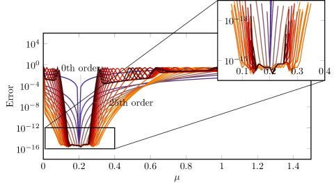
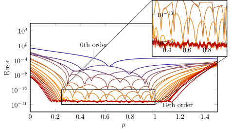
In Figure 2 we compare the difference between the Taylor approximation and the eigenvalues computed after discretizing the parametric eigenvalue problem. We plot the maximum overall eight eigenvalues to declutter the plot. We observe that the 20th Taylor approximation has an error of about $10\epsilon_{\text{mach}}$ in the interval $[0.1,0.3]$.

Due to the factor $(\mu-\mu_{0})^{p}$ the higher Taylor coefficients play a secondary role for the approximation of the eigenvalues for $\mu$ close to the expansion point. However, one can clearly see that for $\mu=0.6$ and for larger $\mu$ an increase in the degree does not provide an improvement of the approximation. This is caused by the accumulation of errors as described above.

To check this hypothesis we have redone the computations for Figure 2 with the only change that the matrix $E$ is rounded to single precision instead of double precision. The results are shown in Figure 3. We can observe that higher order approximations do not improve the quality of the approximation due to the accumulation of errors.

3 Chebyshev Expansion

We observed in the last section that the quality of the Taylor approximations drops quickly if we get further away from the expansion point. This is expected but unsatisfactory. Increasing the degree of the Taylor expansion can increase the interval for which we obtain a satisfactory approximation as seen in Figure 2 and 3. However, as the preliminary numerical experiments above and the ones in Section 4 show, this is limited by the accumulation of errors. Hence, we need a different approach if we are interested in an accurate approximation of $\lambda(\mu)$ over a large interval. We decided to use the Chebyshev expansion of $A(\mu)$, $\lambda(\mu)$, and $v(\mu)$.

Let $\{U_{0}(\mu),U_{1}(\mu),U_{2}(\mu),\dotsc\}$ be an orthonormal basis of Chebyshev polynomials of second kind scaled to the interval $[\mu_{1},\mu_{2}]$. We can then write

$$A(\mu) =A_{0}U_{0}(\mu)+A_{1}U_{1}(\mu)+A_{2}U_{2}(\mu)+\dotsc,$$ (49)

$$\lambda(\mu) =\lambda_{0}U_{0}(\mu)+\lambda_{1}U_{1}(\mu)+\lambda_{2}U_{2}(\mu)+\dotsc,\quad\text{and}$$

$$v(\mu) =v_{0}U_{0}(\mu)+v_{1}U_{1}(\mu)+v_{2}U_{2}(\mu)+\dotsc.$$

In Section 2 we assumed that the $A_{i}$ are given. This makes sense for Example 3 and for other examples since the entry-wise derivative of $A(\mu)$ can be obtained symbolically in an efficient way. For the Chebyshev expansion it is an unlikely situation that the $A_{i}$ are given, i.e. that the matrix $A(\mu)$ is given as polynomial in a Chebyshev basis. Thus we first have to compute them by

$$A_{i}:=\langle A(\mu),U_{i}(\mu)\rangle_{U}:=\int_{\mu_{1}}^{\mu_{2}}A(\mu)\,U_{i}(\mu)\,\frac{2}{\mu_{2}-\mu_{1}}\sqrt{1-\left(\frac{2\mu-\mu_{2}-\mu_{1}}{\mu_{2}-\mu_{1}}\right)^{2}}\,\mathrm{d}\mu.$$ (50)

This can be achieved by a quadrature formula or other standard algorithms. We choose to use the Chebfun package for these computation in our Matlab code. In (50) lies a main difference to the Taylor expansion approach: When using the Taylor expansion $A_{0}$ is equal to $A(\mu_{0})$, while when using Chebyshev $A_{0}$ is a weighted average of $A(\mu)$ in $[\mu_{1},\mu_{2}]$.

Equation (50) defines an inner product in which the Chebyshev basis of second kind is orthonormal, that is

$$\langle U_{i}(\mu),U_{j}(\mu)\rangle_{U}=\delta_{ij}.$$

We can estimate the approximation error by truncating (49) with the help of this inner product

$$A(\mu)= A_{0}U_{0}(\mu)+A_{1}U_{1}(\mu)+A_{2}U_{2}(\mu)+\dotsc+A_{p}U_{p}(\mu)+\Delta_{p}(\mu)$$

$$\mbox{$\parallel\!A(\mu)\!\parallel$}_{U}^{2}:= \langle A(\mu),A(\mu)\rangle_{U}=\sum_{i=0}^{p}\langle A(\mu),U_{i}(\mu)\rangle_{U}+\langle A(\mu),\Delta_{p}(\mu)\rangle_{U}$$

The Chebyshev basis is degree graded with the degree of $U_{i}$ being $i$. Thus the degree of the product $U_{i}U_{j}$ is $i\cdot j$. However, the product is not equal to $U_{ij}$ as it is the case for the basis $T_{i}=(\mu-\mu_{0})^{i}$ used for the Taylor expansion. In fact for Chebyshev polynomials of second kind we have

$$U_{i}U_{j}=U_{i+j}+U_{i+j-2}+\dotsb+U_{\left\lvert i-j\right\rvert+2}+U_{\left\lvert i-j\right\rvert}.$$ (51)

If we ignore all but the first term in (51), then we obtain an equation very similar to (48):

$$\left[\begin{array}[]{cc|cc|cc|cc}0&v_{0}^{T}&&&&&&\\ v_{0}&-A_{0}&&&&&&\\ \hline\cr 0&v_{1}^{T}&0&v_{0}^{T}&&&&\\ v_{1}&-A_{1}&v_{0}&-A_{0}&&&&\\ \hline\cr 0&v_{2}^{T}&0&v_{1}^{T}&0&v_{0}^{T}&&\\ v_{2}&-A_{2}&v_{1}&-A_{1}&v_{0}&-A_{0}&&\\ \hline\cr 0&v_{3}^{T}&0&v_{2}^{T}&0&v_{1}^{T}&0&v_{0}^{T}\\ v_{3}&-A_{3}&v_{2}&-A_{2}&v_{1}&-A_{1}&v_{0}&A_{0}\end{array}\right]\left[\begin{array}[]{c}\lambda_{0}\\ v_{0}\\ \hline\cr\lambda_{1}\\ v_{1}\\ \hline\cr\lambda_{2}\\ v_{2}\\ \hline\cr\lambda_{3}\\ v_{3}\end{array}\right]=\left[\begin{array}[]{c}1\\ 0\\ \hline\cr 0\\ 0\\ \hline\cr 0\\ 0\\ \hline\cr 0\\ 0\end{array}\right].$$

Solving this equation does not give us the correct solution because we made a severe simplification. However, this is an approximation to the solution, which can be computed iteratively and similar to Algorithm 1 due to the block lower triangular structure. We can obtain this approximation also in $O(25n^{3}+p^{2}n^{2})$ for one eigenpair or $O((25+p^{2})n^{3})$ for all eigenpairs.

If we do not ignore the terms in (51), then the system of equations for $p=3$ is

$$\left[\begin{array}[]{cc|cc|cc|cc}0&v_{0}^{T}&0&{\color[rgb]{0.75,0,0}\definecolor[named]{pgfstrokecolor}{rgb}{0.75,0,0}v_{1}^{T}}&&&&\\ v_{0}&-A_{0}&{\color[rgb]{0.75,0,0}\definecolor[named]{pgfstrokecolor}{rgb}{0.75,0,0}v_{1}}&{\color[rgb]{0.75,0,0}\definecolor[named]{pgfstrokecolor}{rgb}{0.75,0,0}-A_{1}}&&&&\\ \hline\cr 0&v_{1}^{T}&0&v_{0}^{T}+{\color[rgb]{0,0,0.75}\definecolor[named]{pgfstrokecolor}{rgb}{0,0,0.75}v_{2}^{T}}&0&{\color[rgb]{1.0,.5625,0}\definecolor[named]{pgfstrokecolor}{rgb}{1.0,.5625,0}v_{1}^{T}}&&\\ v_{1}&-A_{1}&v_{0}+{\color[rgb]{0,0,0.75}\definecolor[named]{pgfstrokecolor}{rgb}{0,0,0.75}v_{2}}&-A_{0}{\color[rgb]{0,0,0.75}\definecolor[named]{pgfstrokecolor}{rgb}{0,0,0.75}-A_{2}}&{\color[rgb]{1.0,.5625,0}\definecolor[named]{pgfstrokecolor}{rgb}{1.0,.5625,0}v_{1}}&{\color[rgb]{1.0,.5625,0}\definecolor[named]{pgfstrokecolor}{rgb}{1.0,.5625,0}-A_{1}}&&\\ \hline\cr 0&v_{2}^{T}&0&{\color[rgb]{0.75,0,0}\definecolor[named]{pgfstrokecolor}{rgb}{0.75,0,0}v_{1}^{T}}&0&v_{0}^{T}&&\\ v_{2}&-A_{2}&{\color[rgb]{0.75,0,0}\definecolor[named]{pgfstrokecolor}{rgb}{0.75,0,0}v_{1}}&{\color[rgb]{0.75,0,0}\definecolor[named]{pgfstrokecolor}{rgb}{0.75,0,0}-A_{1}}&v_{0}&-A_{0}&&\\ \hline\cr 0&v_{3}^{T}&0&{\color[rgb]{0,0,0.75}\definecolor[named]{pgfstrokecolor}{rgb}{0,0,0.75}v_{2}^{T}}&0&{\color[rgb]{1.0,.5625,0}\definecolor[named]{pgfstrokecolor}{rgb}{1.0,.5625,0}v_{1}^{T}}&0&v_{0}^{T}\\ v_{3}&-A_{3}&{\color[rgb]{0,0,0.75}\definecolor[named]{pgfstrokecolor}{rgb}{0,0,0.75}v_{2}}&{\color[rgb]{0,0,0.75}\definecolor[named]{pgfstrokecolor}{rgb}{0,0,0.75}-A_{2}}&{\color[rgb]{1.0,.5625,0}\definecolor[named]{pgfstrokecolor}{rgb}{1.0,.5625,0}v_{1}}&{\color[rgb]{1.0,.5625,0}\definecolor[named]{pgfstrokecolor}{rgb}{1.0,.5625,0}-A_{1}}&v_{0}&A_{0}\end{array}\right]\left[\begin{array}[]{c}\lambda_{0}\\ v_{0}\\ \hline\cr\lambda_{1}\\ v_{1}\\ \hline\cr\lambda_{2}\\ v_{2}\\ \hline\cr\lambda_{3}\\ v_{3}\end{array}\right]=\left[\begin{array}[]{c}1\\ 0\\ \hline\cr 0\\ 0\\ \hline\cr 0\\ 0\\ \hline\cr 0\\ 0\end{array}\right],$$ (76)

where the colored blocks occur multiple times. The system (76) is no longer block lower triangular and thus cannot be solved by forward substitution. We hence fallback on solving this non-linear system by Newton’s method. In each step we have to compute and invert the Jacobi matrix. This is a matrix of size $(p+1)(n+1)$. Thus the costs are in $O(n^{3}p^{3})$ for each Newton step for each eigenvalue. We observe that 4 to 8 Newton steps are typically sufficient, since we already start with a good approximation.

We truncate the series for $A(\mu)$, $\lambda(\mu)$, and $v(\mu)$ all after $p+1$ terms, so that they are all polynomials of degree $p$. Different choice may be possible but we did not see an advantage in using different degrees for $A$, $\lambda$, and $v$ in our preliminary experiments.

Nonlinear systems can have many solutions. However, the special constructions of (76) ensures that every of its solutions represents a Chebyshev approximation of an eigenpair of the parametric eigenvalue problem. For the solution

$$\begin{bmatrix}\lambda_{0}&\phantom{\gamma}v_{0}&\lambda_{1}&\phantom{\gamma}v_{1}&\dotsb&\lambda_{p-1}&\phantom{\gamma}v_{p-1}\end{bmatrix}^{T}$$

there are infinitely many more of the form:

$$\begin{bmatrix}\lambda_{0}&\gamma v_{0}&\lambda_{1}&\gamma v_{1}&\dotsb&\lambda_{p-1}&\gamma v_{p-1}\end{bmatrix}^{T}$$

for all $\gamma$ with $\left\lvert\gamma\right\rvert=1$. Newton’s method does not guarantee that we converge to the closest root of these. Thus, despite starting with $n$ initial approximations, one close to each root, there is no guarantee that we end up with $n$ distinct eigenpairs $(\lambda(\mu),\gamma v(\mu))$ not just differing in $\gamma$.

For polynomial rootfinding this problem can be overcome by the Ehrlich-Aberth method [1, 10], see for instance [5]. This is possible for polynomial rootfinding since the eigenvectors corresponding to each root can be derived easily from said root. Unfortunately, this is not possible here. As a consequence we are left with the hope that the starting vectors are sufficiently close. In the special case that all eigenvalues and eigenvectors are real, there are only two choices for $\gamma$, $\gamma=1$ and $\gamma=-1$. In this case we had some heuristic success in employing the Ehrlich-Aberth method. However, with poorly chosen start-vectors it was still possible to trick the algorithm into finding the same eigenpair twice.

3.1 Accuracy

We now want to discuss the accuracy of the computed and truncated Chebyshev expansions for $\lambda(\mu)$ and $v(\mu)$. The Chebyshev theorem states that the best approximation in the Chebyshev basis $b_{n}$ fulfills

$$f(x)-b_{n}(x)=\frac{f^{(n+1)}(\xi)}{(n+1)!}\prod_{i=0}^{n}(x-z_{i}),$$ (77)

for unknown interpolation points $z_{i}\in[\mu_{1},\mu_{2}]$ and an unknown point $\xi\in[\mu_{1},\mu_{2}]$ [9]. The reason is that the Chebyshev approximation $b_{n}(x)$ intersects with $f(x)$ at $n$ unknown points in $[\mu_{1},\mu_{2}]$. Thus it is an interpolation polynomial at these points and for such an interpolation polynomial (77) holds. We can bound the right-hand side by $(b-a)^{n}\sup_{\xi\in[\mu_{1},\mu_{2}]}\frac{f^{(n+1)}(\xi)}{(n+1)!}$. This is a good bound for the eigenvalues, but for eigenvectors the derivative may be huge when two eigenvalues are near to each other, see [12, Sect. 7.2.2] for details.

Additionally, the Chebyshev coefficients we compute with Newton’s method are perturbed because we only approximate the solution of (76).

3.2 Proof-of-Concept

We repeat the experiments from Section 2.2 based on Example 3 with Chebyshev expansion instead of Taylor series expansion.

Fig. 4: Example 3—Maximal difference between Chebyshev approximations and eigenvalues, $[\mu_{1},\mu_{2}]=[0.25,1.00]$.

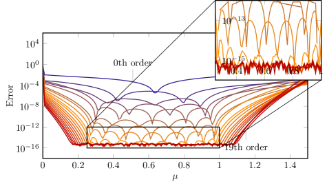
Figure 4 is the Chebyshev version of Figure 2 with Chebyshev expansions on the interval $[\tfrac{1}{4},1]$. Contrary to the Taylor approximation we do not just see a small error near the expansion point but a small error over the whole interval. The error increases slightly towards the endpoints of the intervals, with the error near $1$ being $10^{-13}$, while the error near $\tfrac{1}{4}$ is closer to $10^{-14}$. Outside the approximation interval the error increases the further we are from the endpoints. Here, we do not observe that an increase in the order leads to worse results, since the use of Newton’s method to solve the nonlinear equation gets us around the error accumulation problem. However, in Figure 8 depicting the error in the eigenvectors, we observe that the error outside the approximation interval increases for large $p$.

4 Numerical Experiments

In the last section we used Example 3 to verify that the proposed methods work for the arguably most easy problem of symmetric positive definite matrices. In this section we will present further experiments for other examples.

Fig. 5: Example 4—Sketch of the springs and masses.

Example 4.

We investigate a sequence of masses connected with springs as in Figure 5. All springs have a stiffness of $1$. All but two masses in the middle have mass $1$. The two masses in the middle are both of mass $\mu$. This example is an extreme simplification of a passenger of unknown mass in a car.

This problem leads to a generalized eigenvalue problem dependent on $\mu$. As mentioned earlier generalized eigenvalue problems are significantly more difficult to handle with the expansion approaches. Thus we choose to turn the problem into a standard eigenvalue problem. Inversion of the mass matrix leads to

$$A(\mu)=\begin{bmatrix}1\\ &\smash{\ddots}\\ &&1\\ &&&\mu\\ &&&&\mu\\ &&&&&1\\ &&&&&&\smash{\ddots}\\ &&&&&&&1\\ \end{bmatrix}^{-1}\begin{bmatrix}2&-1\\ -1&\smash{\ddots}&\smash{\ddots}\\ &\smash{\ddots}&2&-1\\ &&-1&2&-1\\ &&&-1&2&-1\\ &&&&-1&2&\smash{\ddots}\\ &&&&&\smash{\ddots}&\smash{\ddots}&-1\\ &&&&&&-1&2\\ \end{bmatrix}.$$

Thus only two rows of $A(\mu)$ are dependent on $\mu$.

The matrix $A(\mu_{0})$ is not symmetric in this example. However, using the square root of the mass matrix would permit to construct a symmetric problem instead.

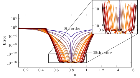
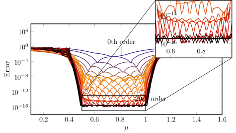
We apply Algorithm 1 with $\mu_{0}=0.8$ and its Chebyshev sibling for the interval $[\mu_{1},\mu_{2}]=[0.5,1.0]$ to Example 4. The resulting eigenvalues are depicted in Figure 6. Figure 7 shows the error of the Taylor approximation to sampled eigenvalues. Figure 8 does the same for the Chebyshev approximation. We observe that in this example we need a higher order for the Chebyshev approximation than for the Taylor approximation in order to obtain the same level of accuracy. However, the Chebyshev approximation is better over a larger interval. The example demonstrates that the technique computing the Chebyshev approximation does not suffer from an accumulation of errors and thus we can compute the higher order approximation sufficiently accurate. It also shows that the Chebyshev approximation is of good quality in the inner part of the interval $[\mu_{0},\mu_{1}]$. However, near the endpoints the quality deteriorates significantly.

Fig. 6: Example 4, $n=8$, $\mu_{0}=0.80$ and $[\mu_{1},\mu_{2}]=[0.50,1.00]$, respectively.

Fig. 7: Example 4—Maximal difference between Taylor approximations and eigenvalues, $\mu_{0}=0.80$.

Fig. 8: Example 4—Maximal difference between Chebyshev approximations and eigenvalues, $[\mu_{1},\mu_{2}]=[0.50,1.00]$.

The examples we looked at so far had a full set of eigenvectors for all parameter values in the interval of interest. The following examples uses a basic Jordan block to test the algorithm for an example with defective eigenvalues.

Example 5.

We use a Jordan block with a parameter in the lower left corner, that is

$$A(\mu)=\begin{bmatrix}1&1&&&0\\ 0&1&1\\ \vdots&\ddots&\ddots&\ddots\\ 0&\cdots&0&1&1\\ \mu&0&\cdots&0&1\end{bmatrix}$$

The eigenvalues of $A(\mu)$ are the roots of the characteristic polynomial

$$p(\lambda,\mu)=(\lambda-1)^{n}-\mu.$$

The roots are the unit roots $\rho_{1},\dotsc,\rho_{n}$ of $\rho^{n}=-1$ scaled by $\mu^{1/n}$ and shifted by $1$ to the right.

We note that we primarily focused our algorithms on the case of non-defective, preferable positive definite matrices, which Example 5 is very much not. Nevertheless we are interested in how far the techniques described in this paper produce meaningful results in this case.

We apply Algorithm 1 with $\mu_{0}=0.2$ and $\mu_{0}=-0.2$ and its Chebyshev sibling with $[\mu_{1},\mu_{2}]=[0.5,1.0]$ to Example 5. The real and imaginary parts of the Taylor approximation eigenvalues are depicted in Figure 9 for $\mu_{0}=0.2$. A similar figure can be obtained for $\mu_{0}=-0.2$. We observe that the Taylor series approximations do not provide useful approximations beyond the singularity at $\mu=0$. This is expected, since the eigenvalues are not analytic at $\mu=0$. Algorithm 1 failed for the expansion point $\mu_{0}=0$.

Using the Chebyshev approximation we observe a very similar behavior, see Figure 10. The algorithm failed to provide a meaningful approximation when $0\in[\mu_{1},\mu_{2}]$. The Chebyshev approximation is also not capable of approximating the eigenvalues beyond $0$.

Fig. 9: Example 5, $n=8$, $\mu_{0}=0.20$.

Fig. 10: Example 5, $n=8$, $[\mu_{1},\mu_{2}]=[0.10,0.50]$.

4.1 Assessing the Quality of the Eigenvector Approximation

We are now going to assess the quality of the eigenvector approximation. We use the Taylor and Chebyshev approximation of the eigenvectors, respectively. We observe that despite our efforts to produce normalized eigenvectors, the function values $v(\mu)$ are not of norm $1$. In particular, the Chebyshev approximation techniques produces eigenvectors far from norm $1$. For our comparison we evaluate the function $v(\mu)$ for a particular $\mu$ and then normalize the result before comparing it to the normalized eigenvectors of $A(\mu)$.

We fix $\mu_{j}$. Let $V_{s}$ be the matrix of eigenvectors of $A(\mu_{j})$ with $A(\mu_{j})V_{s}=D_{s}V_{s}$, with $D_{s}$ diagonal, and let $V$ be the result of the normalization of $v(\mu_{j})$. We use the Matlab command max(abs(max(abs(Vs’*V))-1)) to compute the maximum deviation of the eigenvectors for $\mu_{j}$.

Figure 11–14 show the deviation of the eigenvectors for Example 3 and 4. We observe in Figure 11 and Figure 14 that increasing the order of approximation provides diminishing returns and eventually a decrease in approximation quality.

Surprisingly, Figure 13 shows that order 10 is sufficient to approximate the eigenvectors with the Chebyshev approach well, while Figure 4 shows that we need a higher order to approximate the eigenvalues well. Knowing the eigenvectors $v(\mu_{i})$ for a given $\mu_{i}$ and a known matrix $A(\mu_{i})$ allows to compute an approximation to the eigenvalues $\lambda(\mu_{i})$ using the Rayleigh quotient. It is a well known fact that for symmetric matrices an approximation $q$ to the eigenvector $v$ with $\mbox{$\parallel\!q-v\!\parallel$}=O(\delta)$ implies that the Rayleigh quotient $\rho=q^{T}Aq/q^{T}q$ approximates the eigenvalue $\lambda$ to $v$ with $\left\lvert\lambda-\rho\right\rvert=O(\delta^{2})$, see for instance [29, Exercise 5.4.33]. Thus for symmetric matrices using the eigenvector approximation together with the Rayleigh quotient is very likely going to produce a better approximation to the eigenvalue. This is aided by the fact that for the Rayleigh quotient one can use the exact $A(\mu)$. We tried this out and found a better approximation than using $\lambda(\mu_{i})$, cp. Figure 15 with Figure 4.

Fig. 11: Example 3—Maximal difference between Taylor approximations and eigenvectors, $\mu_{0}=0.20$.

Fig. 12: Example 4—Maximal difference between Taylor approximations and eigenvectors, $\mu_{0}=0.80$.

Fig. 13: Example 3—Maximal difference between Chebyshev approximations and eigenvectors, $[\mu_{1},\mu_{2}]=[0.25,1.00]$.

Fig. 14: Example 4—Maximal difference between Chebyshev approximations and eigenvectors, $[\mu_{1},\mu_{2}]=[0.50,1.00]$.

Fig. 15: Example 3—Maximal difference between Rayleigh quotient of the Chebyshev eigenvector approximations and the eigenvalues, $[\mu_{1},\mu_{2}]=[0.25,1.00]$.

4.2 Sampling

We have presented a method to find approximations to $\lambda(\mu)$. These approximations can be used to speed-up the following sampling process: Assume a distribution of $\mu$ is given and can be sampled. For the following tests we use $\mu\sim\mathcal{N}(\mu_{0},0.01)$, that is normally distributed around $\mu_{0}=0.2$ with standard deviation $0.1$. We can thus produce samples $\mu_{i}$ and use these to compute samples $\lambda(\mu_{i})$ of the distribution of the eigenvalues. In the example below the second and third largest eigenvalue are sampled. This is faster than computing $A(\mu)$ and then using a standard eigenvalue algorithm to compute the eigenvalues of $A(\mu)$. For $10,000$ samples using Example 3 with $n=8$ and approximations of $6$th order we observed that $3.6938$ s were spend on forming the matrix as a function, $0.0096$ s were spend on solving (1) with the Taylor approximation and $0.1464$ s with the Chebyshev approximation. For sampling the eigenvalues using the full matrix $A(\mu)$ $1.6386$ s were needed, while sampling with the obtained Taylor (using Horner’s method) and Chebyshev approximations could be done in $0.0807$ s and $0.0616$ s, respectively. Thus the sampling was done 20.3 and 26.6 times faster, respectively, or 18.14 and 7.87 times faster if the one-time costs for solving (1) are added to the costs for the sampling. The more accurate results obtained through the Rayleigh quotient are slightly more expensive and, thus, are only 5.58 and 5.89 times faster, respectively. We summarize these numbers together with the theoretical complexities in Table 3.

Table 3: Comparing direct sampling of $s=10,000$ eigenvalues of $A(\mu)$ with first computing a Taylor or Chebyshev expansion, for $A(\mu)\in\mathbb{R}^{n\times n}$, with $n=8$ and $p=6$.

		Taylor	Chebyshev	direct sampling
setup	theoretical costs	$O((25+p^{2})n^{3})$	$O(n^{4})$	—
	runtime	0.0096 s	0.1464 s	—
sampling	theoretical costs	$O(ps)$	$O(ps)$	$O(sn^{3})$
	runtime	0.0807 s	0.0616 s	1.6386 s
	speed up	20.3$\times$	26.6$\times$	—
	with Rayleigh quot.	0.2838 s	0.1319 s	—
	speed up	5.77$\times$	12.4$\times$	—
combined	runtime	0.0903 s	0.2080 s	1.6386 s
	speed up	18.14$\times$	7.87$\times$	—
	with Rayleigh quot.	0.2934 s	0.2783 s	—
	speed up	5.58$\times$	5.89$\times$	—

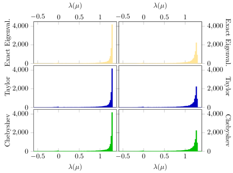
With the help of the sampling we generated the histogram plots in Figure 16. The histogram plots appear visually very similar and can be used to obtain a general impression of the distribution. In particular for $\mu$ far from $\mu_{0}$ or from $[\mu_{1},\mu_{2}]$ the approximation quality is low.

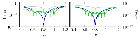
We also plotted $\lambda(\mu)$ over $\mu$ (   ) in Figure 17 together with the error. We observe that the Taylor approximation (   ) provides a good approximation near $\mu_{0}$, while the Chebyshev approximation (   ) is better over the whole interval $[\mu_{1},\mu_{2}]$. We can again observe that the Rayleigh quotient can be used to improve the approximation to $\lambda(\mu)$ for both the Taylor and the Chebyshev approximation; dashed lines  and  , respectively. However, this improvement only works for symmetric matrices, like Example 3. Figure 18 presents the last row of Figure 17 but for the non-symmetric Example 4, and hence, there is only a minor or no improvement visible when using the Rayleigh quotient approximation.

Fig. 16: Example 3—Histogram plot of eigenvalue distribution second and third largest eigenvalue, $6$th order Taylor approximation with $\mu_{0}=0.20$ and $6$th order Chebyshev approximation with $[\mu_{1},\mu_{2}]=[0.1,0.3]$.

Fig. 17: Example 3—$\lambda(\mu)$ over $\mu$ second (left) and third largest eigenvalue (right), exact eigenvalue (orange line  ), $6$th order Taylor approximation with $\mu_{0}=0.20$ (solid blue line  ), and $6$th order Chebyshev approximation eigenvalue (solid green line  ) with $[\mu_{1},\mu_{2}]=[0.1,0.3]$; and eigenvalue approximation using the Rayleigh quotient based on the eigenvector approximation (dashed lines  and   ). For comparison the Rayleigh quotient $v(\mu_{0})^{T}A(\mu)v(\mu_{0})/v(\mu_{0})^{T}v(\mu_{0})$ (grey line  ).

Fig. 18: Example 4—$\lambda(\mu)$ over $\mu$ second (left) and third largest eigenvalue (right), $6$th order Taylor approximation with $\mu_{0}=0.80$ (solid blue line  ), and $6$th order Chebyshev approximation eigenvalue (solid green line  )) with $[\mu_{1},\mu_{2}]=[0.6,1.0]$; and eigenvalue approximation using the Rayleigh quotient based on the eigenvector approximation (dashed lines  and   ). For comparison the Rayleigh quotient $v(\mu_{0})^{T}A(\mu)v(\mu_{0})/v(\mu_{0})^{T}v(\mu_{0})$ (grey line  ).

5 Conclusions

We have presented a Taylor approximation based method to compute approximations to $\lambda(\mu)$ and $v(\mu)$ for the parametric eigenvalue problem (1). The presented algorithm works for small degrees $p$ and the investigated examples. The algorithm accumulates the errors when increasing the degree $p$. Together with the errors present in $E$ when forming the matrix in double (or single) precision, this leads to a serious limitation regarding the maximum degree $p_{\max}$. This limits the usefulness of this approach to a small neighborhood around $\mu_{0}$. We were able to verify that the runtime complexity of this algorithm is within the expectations set by counting the number of flops. The algorithm computes all eigenvalues in $O((25+p^{2})n^{3})$.

To overcome the limitations we extended the approach to Chebyshev approximation. This requires the solution of a non-linear system with Newton’s method. The Chebyshev approach has higher costs. Despite a good starting point for the Newton iteration, there is no guarantee that all eigenvalues can be found. However, in the experiments the Chebyshev approximations are superior to the Taylor approximations, in particular since a high accuracy can be achieved over a given interval and not just in the neighborhood of an expansion point. We showed that the method can be used for the sampling of eigenvalues if a distribution of the parameter is given. Depending on the number of sampling points the method presented here can be significantly faster than Monte-Carlo methods.

Availability of data and materials

The code used for the numerical experiments is available from GitHub, https://github.com/thomasmach/PEVP_with_Taylor_and_Chebyshev.

References

- [1] O. Aberth, Iteration methods for finding all zeros of a polynomial simultaneously, Math. Comp., 27 (1973), pp. 339–344.
- [2] M. M. Alghamdi, D. Boffi, and F. Bonizzoni, A greedy MOR method for the tracking of eigensolutions to parametric elliptic PDEs, arXiv preprint arXiv:2208.14054, (2022).
- [3] A. L. Andrew, K.-W. E. Chu, and P. Lancaster, Derivatives of Eigenvalues and Eigenvectors of Matrix Functions, SIAM J. Matrix Anal. Appl., 14 (1993), pp. 903–926.
- [4] T. Betcke, N. J. Higham, V. Mehrmann, C. Schröder, and F. Tisseur, NLEVP: A collection of nonlinear eigenvalue problems, ACM Trans. Math. Software, 39 (2013), pp. 1–28.
- [5] D. A. Bini and L. Robol, Solving secular and polynomial equations: A multiprecision algorithm, J. Comput. Appl. Math., 272 (2014), pp. 276–292.
- [6] L. Bungert and P. Wacker, Complete Deterministic Dynamics and Spectral Decomposition of the Linear Ensemble Kalman Inversion, arXiv preprint arXiv:2104.13281, (2022).
- [7] Y. Cai, L.-H. Zhang, Z. Bai, and R.-C. Li, On an eigenvector-dependent nonlinear eigenvalue problem, SIAM J. Matrix Anal. Appl., 39 (2018), pp. 1360–1382.
- [8] R. Claes, E. Jarlebring, K. Meerbergen, and P. Upadhyaya, Linearizability of eigenvector nonlinearities, arXiv preprint arXiv:2105.10361, (2021).
- [9] V. K. Dzyadyk, Approximation Methods for Solutions of Differential and Integral Equations, VSP, Utrecht, 1995.
- [10] L. W. Ehrlich, A modified Newton method for polynomials, Commun. ACM, 10 (1967), pp. 107–108.
- [11] R. Ghanem and D. Ghosh, Efficient characterization of the random eigenvalue problem in a polynomial chaos decomposition, Int. J. Numer. Methods Eng., 72 (2007), pp. 486–504.
- [12] G. H. Golub and C. F. Van Loan, Matrix Computations, Johns Hopkins University Press, Baltimore, 4th ed., 2013.
- [13] W. Govaerts and J. D. Pryce, Block elimination with one refinement solves bordered linear systems accurately, BIT, 30 (1990), pp. 490–507.
- [14] B. Haasdonk and H. Burkhardt, Invariant kernel functions for pattern analysis and machine learning, Mach. Learn., 68 (2007), pp. 35–61.
- [15] R. A. Horn and C. R. Johnson, Topics in Matrix Analysis, Cambridge University Press, Cambridge, 1991.
- [16] E. Jarlebring, S. Kvaal, and W. Michiels, An inverse iteration method for eigenvalue problems with eigenvector nonlinearities, SIAM J. Sci. Comput., 36 (2014), pp. A1978–A2001.
- [17] E. Jarlebring and P. Upadhyaya, Implicit algorithms for eigenvector nonlinearities, Numer. Algorithms, (2021), pp. 1–21.
- [18] T. Kato, Perturbation Theory for Linear Operators, Springer, Berlin, 1976.
- [19] V. Mehrmann and H. Voss, Nonlinear eigenvalue problems: A challenge for modern eigenvalue methods, GAMM-Mitteilungen, 27 (2004), pp. 121–152.
- [20] C. B. Moler and G. W. Stewart, An algorithm for generalized matrix eigenvalue problems, SIAM J. Numer. Anal., 10 (1973), pp. 241–256.
- [21] M. L. Parks, E. de Sturler, G. Mackey, D. D. Johnson, and S. Maiti, Recycling Krylov subspaces for sequences of linear systems, SIAM J. Sci. Comput., 28 (2006), pp. 1651–1674.
- [22] S. Rahman, A solution of the random eigenvalue problem by a dimensional decomposition method, Int. J. Numer. Methods Eng., 67 (2006), pp. 1318–1340.
- [23] F. Rellich, Störungstheorie der Spektralzerlegung, Math. Ann., 116 (1939), pp. 555–570.
- [24] K. Ruymbeek, K. Meerbergen, and W. Michiels, Tensor-Krylov method for computing eigenvalues of parameter-dependent matrices, J. Comput. Appl. Math., 408 (2022), 113869.
- [25] K. M. Soodhalter, Block Krylov subspace recycling for shifted systems with unrelated right-hand sides, SIAM J. Sci. Comput., 38 (2016), pp. A302–A324.
- [26] B. Sousedik and H. C. Elman, Inverse subspace iteration for spectral stochastic finite element methods, SIAM/ASA J. Unvertain. Quantif., 4 (2016), pp. 163–189.
- [27] F. Tisseur and K. Meerbergen, The quadratic eigenvalue problem, SIAM Rev., 43 (2001), pp. 235–286.
- [28] C. V. Verhoosel, M. A. Gutiérrez, and S. J. Hulshoff, Iterative solution of the random eigenvalue problem with application to spectral stochastic finite element systems, Int. J. Numer. Methods Eng., 68 (2006), pp. 401–424.
- [29] D. S. Watkins, Fundamentals of Matrix Computations, Pure and Applied Mathematics, John Wiley & Sons, Inc., New York, third ed., 2010.
- [30] M. M. R. Williams, A method for solving stochastic eigenvalue problems, Appl. Math. Comput., 215 (2010), pp. 3906–3928.
- [31] , A method for solving stochastic eigenvalue problems II, Appl. Math. Comput., 219 (2013), pp. 4729–4744.