Reducing SO(3) Convolutions to SO(2) for Efficient Equivariant GNNs
Abstract
Graph neural networks that model 3D data, such as point clouds or atoms, are typically desired to be equivariant, i.e., equivariant to 3D rotations. Unfortunately equivariant convolutions, which are a fundamental operation for equivariant networks, increase significantly in computational complexity as higher-order tensors are used. In this paper, we address this issue by reducing the convolutions or tensor products to mathematically equivalent convolutions in . This is accomplished by aligning the node embeddings’ primary axis with the edge vectors, which sparsifies the tensor product and reduces the computational complexity from to , where is the degree of the representation. We demonstrate the potential implications of this improvement by proposing the Equivariant Spherical Channel Network (eSCN), a graph neural network utilizing our novel approach to equivariant convolutions, which achieves state-of-the-art results on the large-scale OC-20 and OC-22 datasets.
1 Introduction
In many domains, it is desired that machine learning models obey specific constraints imposed by the task. A common constraint is equivariance to specific operations on the inputs (Bronstein et al., 2021). That is, if the input is transformed in a certain manner, such as translated or rotated, the output should be transformed appropriately. Prominent examples include equivariance to translations for object detection in images (Girshick et al., 2014), and equivariance to rotations of 3D point clouds (Weiler et al., 2018; Satorras et al., 2021). Machine learning models impose equivariance to a group of symmetries by constraining the operations that can be performed. Namely, the class of functions that can be learned is narrowed to those that are equivariant. The hope is that equivariance will provide a robust prior that can increase data efficiency, improve generalization and eliminate the need for data augmentation (Reisert & Burkhardt, 2009).
-Equivariant graph neural networks (GNNs) have showed great promise in processing geometrical information, such as 3D point clouds of objects (Weiler et al., 2018; Chen et al., 2021) or atoms (Batzner et al., 2022; Thomas et al., 2018; Brandstetter et al., 2022; Liao & Smidt, 2023; Musaelian et al., 2023). These networks incorporate the inherent symmetry in their domains to , the group of 3D rotations. Specifically, they take advantage of geometric tensors of irreducible representations, so-called irreps, to act as node embeddings and utilize directional information. The building block of these networks is an approach to message passing that uses equivariant convolutions based on tensor products of the irreps. Unfortunately, the full tensor product using irreps up to degree have a computational complexity of , which significantly limits their use with degrees higher than 2 or 3.
In this paper, we address this issue by proposing an efficient method to perform equivariant convolutions. Our main observation is that node irreps exhibit special properties if the irreps’ primary axis is aligned to the edge’s direction during message passing. While SCN (Zitnick et al., 2022) observed that this leads to a subset of the coefficients becoming invariant, we demonstrate the benefits extend even further. Specifically, the tensor product becomes sparse, which reduces its computational complexity from to , and removes the need to compute the Clebsch-Gordan coefficients. This enables computationally efficient equivariant models that use irreps of significantly higher degree.
Additionally, we shed light on this novel approach by revealing its relationship with convolutions (Worrall et al., 2017). In fact, while predicting per-atom forces in atomic systems is a -equivariant task, during message passing the symmetry of the problem gets reduced to . Specifically, by aligning the irreps’ primary axis with the edge’s direction, only a single degree of rotational freedom remains. Thus, the irreps can be projected to the analogous irreducible representations of and the much more computationally efficient convolutions may be performed. In conclusion, the tensor product may be viewed as a set of generalized convolutions in if the irreps are rotated appropriately.
We use these insights to propose the Equivariant Spherical Channel Network (eSCN), an equivariant GNN utilizing the efficient implementation of the equivariant convolutions. Empirically, we evaluate our model to the task of predicting atomic energies and forces, a foundational problem in chemistry and material science with numerous important applications; including tackling climate change (Zitnick et al., 2020; Rolnick et al., 2022). Typically, atomic forces and energies are estimated using Density Functional Theory (Hohenberg & Kohn, 1964; Kohn & Sham, 1965), a very computationally expensive calculation; thus, the goal is to approximate DFT through Machine learning models to significantly reduce this cost. We compare eSCN to state-of-the-art GNNs on the large-scale OC-20 and OC-22 datasets (Chanussot et al., 2021), which contain over 100 million atomic structure training examples for catalysts to help address climate change. eSCN achieves state-of-the-art performance across many tasks, especially those such as force prediction ( and improvement for OC-20 and OC-22) and relaxed structure prediction ( improvement) that require high directional fidelity.
2 Related work
Incorporating symmetries of the data in machine learning models can improve their data-efficiency and ability to generalize (Cohen & Welling, 2016). Group theory is a formalism to axiomatically define symmetries (Bronstein et al., 2021). A group is a set of elements with an operation . It acts on a vector space (i.e. for some ) with an operation called group action. We say that is:
-
1.
-Invariant if ,
-
2.
-Equivariant if ,
For our task, we are especially interested in , the group of rotations of . In fact, 3D symmetries are intertwined with the law of physics describing quantum interactions, i.e. the Schrodinger equations (Schrödinger, 1926). Specifically, if we rotate a system the energy should not vary, -invariance, and forces should rotate accordingly, -equivariance.
While equivariance is desired in , equivariant models (Weiler et al., 2018; Goodman & Wallach, 2000; Deng et al., 2021; Puny et al., 2022) use atom embeddings in spaces of much higher dimension. In particular, they use irreps corresponding to the coefficients of the real spherical harmonics, which represent a function on a sphere. Given a set of coefficients , we define a spherical function as:
| (1) |
where is a unit vector indicating the orientation and are the real spherical harmonic basis functions defined over degrees and orders .
Spherical harmonics have the special property that they are steerable, i.e., there exists a Wigner D-matrix of size for 3D rotation for which:
| (2) |
This is the fundamental property for extending the concept of group action to the spherical harmonics’ coefficients:
| (3) |
2.1 Machine learning potentials
Classically, the prediction of a molecule’s energy and forces (Behler, 2016) using machine learning relied on hand-crafted representations (Behler, 2016) like MMFF94 (Halgren, 1996) and sGDML (Chmiela et al., 2018). The research on machine learning potentials has recently moved towards end-to-end learnable models based on graph neural networks (Kipf & Welling, 2017; Gori et al., 2005).
Early work on GNNs focuses on models that extract scalar representations from the atoms’ positions. They achieve equivariance to rotations by utilizing only invariant features. CGCNN (Xie & Grossman, 2018) and SchNet (Schütt et al., 2018) use pair-wise distances, DimeNet (Gasteiger et al., 2020b), SphereNet (Liu et al., 2022) and GemNet (Gasteiger et al., 2021, 2022) extend this to explicitly capture triplet and quadruplet angles.
More recently, equivariant models (Batzner et al., 2022) have surpassed invariant GNNs on small molecular datasets including MD17 (Chmiela et al., 2017) and QM9 (Ramakrishnan et al., 2014). These models build upon the concepts of steerability and equivariance introduced by Cohen and Welling (Cohen & Welling, 2016). They use geometric tensors as node embeddings and ensure equivariance to by placing constraints on the operations that can be performed (Kondor et al., 2018; Fuchs et al., 2020). Specifically, they compute linear operations with a generalized tensor product between the atom embeddings and edges’ directions. In particular, Tensor Field Networks (Thomas et al., 2018), NequIP (Batzner et al., 2022), SEGNN (Brandstetter et al., 2022), MACE (Batatia et al., 2022), Allegro (Musaelian et al., 2023) and Equiformer (Liao & Smidt, 2023) lie in this category, and they are commonly referred to as e3nn networks. Most recently, SCN (Zitnick et al., 2022) have surpassed invariant GNNs on the large-scale OC-20 (Chanussot et al., 2021) dataset. While it represents atoms’ embeddings by geometric tensors, SCN doesn’t strictly enforce equivariance and doesn’t compute any tensor product.
2.2 e3nn networks
In e3nn networks (Geiger & Smidt, 2022), an atom ’s embedding is encoded using the spherical harmonic coefficients where , and is the number of channels. Assuming a fixed number of channels over different degrees of the spherical harmonics, the size of the embedding for each atom is . These embeddings are referred to as irreps, since they rotate following the Wigner D-matrices which are the irreducible representations of (Goodman & Wallach, 2000).
The proper use of the irreps constrains the networks’ operations to be -equivariant. The building block of the message passing between two neighboring atoms and is the result of an equivariant convolution, which are summed across neighboring atoms to obtain the updated embedding :
| (4) |
The convolutions are obtained by computing a generalized tensor product between the input embedding and the edge direction (filter), . The values of of degree are obtained as a sum of irreps:
| (5) |
is a learnable non-linear function that takes as input the distance between the atoms and their atomic numbers and , and outputs a scalar coefficient.
For fixed integer values of , and , the generalized tensor product is a bilinear equivariant operation that takes as input an irrep of degree and a filter irrep of degree and outputs an irrep of degree . We can compute the tensor product of Equation (5) using the Clebsch-Gordan coefficients (Griffiths & Schroeter, 2018) as follows:
| (6) |
The values of and of the tensor product in Equation (5) are specified in the architecture of the model and are non-zero for . Retaining all the non-zero tensor products up to degree becomes computationally unfeasible as we scale since it requires 3D matrix multiplications. Therefore most e3nn networks are limited to the computation of or and or .
3 Efficient equivariant convolution
The computational complexity of performing a full tensor product makes it extremely expensive to use degrees higher than or . For many applications, such as modeling systems of atoms, high-fidelity of angular information is critical for modeling their interactions. Next, we demonstrate how to dramatically speed up these calculations for higher degrees.
Let be an -equivariant function, then the following holds for any Wigner-D rotation matrix , rotation matrix and irreps of degree :
| (7) |
Combining Equations (2), (7) with (5) we find:
| (8) |
where and .
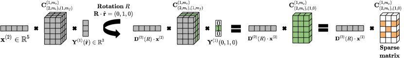
We can now present our key observation. By choosing a specific , we can reduce the cost of computing Equation (8) substantially. Specifically, if we select a rotation matrix so that , we find becomes sparse:
| (9) |
Note that this observation is widely used in computational electromagnetics; specifically for the fast multipole method, this is known as the point-and-shoot method for calculating translation operators (Wala & Klöckner, 2020).
Substituting Equation (9) into the right-hand side of Equation (8) results in the following:
| (10) |
This reduces significantly the amount of computation for the tensor product since we don’t need to sum over in Equation (6):
| (11) |
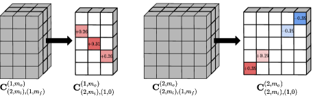
However, even further computational efficiency gains may be achieved. The Clebsch-Gordan matrix of Equation (11) is sparse and follows a particular pattern; see Appendix A.1 for the proof.
Proposition 3.1.
The coefficient is non-zero only if . Moreover and

Therefore the Clebsch-Gordan coefficients can be compactly described using the following notation:
| (12) |
We further simplify the right-hand side of Equation (10) using the result in Proposition 3.1 and the notations introduced above obtaining:
| (13) |
where is defined by the following Equations:
| (14) |
and satisfies:
| (15) |
We prove in Appendix A.2 that the scalar coefficients are related to with a linear bijection. Therefore the model can directly parametrize without loosing or adding any information.
The new formulation of the equivariant convolution provided in Equation (14) doesn’t pre-compute the Clebsch-Gordan coefficients and is drastically more efficient since we no longer sum over , and .
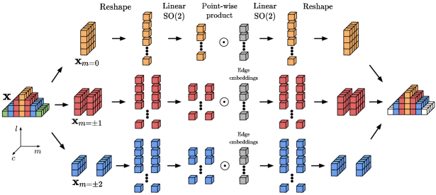
In Appendix C, we provide a theoretical analysis on the computational complexity of the equivariant convolutions; specifically, we show that the computational cost of performing a full tensor product scales with , whereas our efficient approach is . Moreover we show how the new formulation of the equivariant convolutions can be efficiently parallelized on a GPU by reshaping the irreps to group coefficients of the same order m together. This allows to perform a separate convolution for each order m by parametrizing only two dense linear transformations. Note that for higher m close to , the GPU may not be fully utilized as the number of coefficients decreases, but this doesn’t happen in practice since we typically restrict to or .
4 SO(2) formulation
In the previous section, we described how the computation of the generalized tensor product can be greatly simplified. Here we propose an alternative explanation of the same operation as a reduction from -equivariance to -equivariance. Previously, we simplified the generalized tensor product by first rotating the spherical harmonic coefficients so that the primary axis (y-axis) was aligned with the direction of messages’s source atom to the target atom , . Intuitively, once this axis is fixed, only a single rotational degree of freedom remains; the roll rotation over . Thus, if the message passing function is -equivariant to the roll rotation about , it will also be -equivariant.
To see this mathematically, let us define the circular harmonics, which are the representation analogous to spherical harmonics in . A circular harmonic of degree and order is defined as:
| (16) |
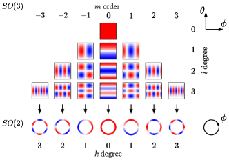
The real spherical harmonics basis functions used in Equation (1) can be written as:
| (17) |
where is the Legendre polynomial which depends only on the colatitude angle and is the longitude angle, i.e., the rotation about the y-axis. Note that and may be computed directly from . Combining Equations (1), (16) and (17) we find the spherical function can be rewritten as:
| (18) |
where if and 1 otherwise. Using our proposed approach, if atoms are rotated in 3D, only the angle will change since is fixed by aligning to the y-axis. As a result, Equation (18) is equivalent to a sum of 2D circular harmonics and becomes a coefficient of . Additionally, the circular harmonics themselves are a Fourier series; as such, a convolution about , which is equivariant (Worrall et al., 2017), may be performed using a simple point-wise product in the spectral domain (Bocher, 1906):
| (19) |
Furthermore, we can generalize the convolution about adding self-interactions between different circular channels as follows:
| (20) |
We finally note that the above Equation coincides with tensor product of Equation (14) when we let . In conclusion, the generalized tensor product of Equation (4) may be viewed as a set of generalized convolutions in if the spherical harmonic coefficients are rotated appropriately.
5 Architecture
Given an atomic structure with atoms, our goal is to predict the structure’s energy and the per-atom forces for each atom . These values are estimated using a Graph Neural Network (GNN) where each node represents an atom and edges represent nearby atoms. As input, the network is given the vector distance between atom and atom , and each atom’s atomic number . The neighbors for an atom are determined using a fixed distance threshold with a maximum number of neighbors set to 20.
Each node ’s embedding is a set of irreps , where is indexed by , and . is the -th component (order) of the -th channel of an irrep of degree .
is initialized with an embedding based on the atomic number and are set to for . The nodes’ embeddings are updated by the GNN through message passing for layers to obtain the final node embeddings. The nodes’ embeddings are updated by first calculating a set of messages for each edge, which are then aggregated at each node. Finally, the energy and forces are estimated from the nodes’ final embeddings.
Our model follows the architecture of SCN (Zitnick et al., 2022), except we replace the message passing operation with our equivariant approach. The message aggregation and output blocks remain the same as SCN. While not novel, we describe for completeness the message aggregation and output blocks in Sections 5.2 and 5.3.
5.1 Message passing
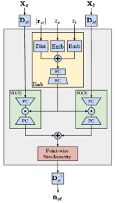
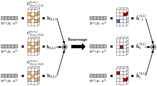
Given a target node and its neighbors , we want to update the embeddings at each layer . The message passing architecture can be divided into three different parts: 1) An edge embedding block that computes an embedding from invariant edge information, 2) a block that performs the generalized convolution in , 3) a point-wise spherical non-linearity performed on the sphere. In Figure 5 and 6 we illustrate the message passing architecture and a tensor representation of the block.
Edge embedding block. It takes as input the distance and the atomic numbers and , and outputs two invariant embeddings per order of size . The atomic numbers and are used to look up two independent embeddings of size , and a set of 1D basis functions are used to represent using equally spaced Gaussians every from to the with followed by a linear layer. Their values are added together and passed through a two-layer neural network with non-linearities to produce the embeddings. They are fed into the block.
SO(2) block. The model computes two independent equivariant convolutions for and . As described previously for enabling efficient calculations, the atoms’ embeddings are rotated to align the direction to the y-axis. The rotations are performed using the Wigner D-matrices so that . The generalized convolutions are performed on all coefficients up to order . For each , there are coefficients with channels. Instead of doing a large dense linear layer to perform the generalized convolution, we linearly project the coefficients down to a hidden layer. The hidden layer values are multiplied by the invariant edge embeddings to incorporate the edge information and then linearly expanded back to the original layer size of . The implementation of the convolutions inherently calculates two linear layers, used to update the values of the the and coefficients as described in Equation (14). Note that as we demonstrate later, may be less than with minimal loss in accuracy while improving efficiency. The ability to use smaller may be due to a couple of reasons. First, larger have fewer coefficients, i.e., the number of coefficients for a specific is . Second, after the coefficients are rotated to align with an edge, larger encode the higher frequency information perpendicular to the edge’s direction, which may be less informative than information parallel to the edge’s direction.
Point-wise spherical non-linearity. The result of the two blocks are added together and a point-wise spherical non-linearity is performed:
| (21) |
A point-wise function is an equivariant operation since it performs the same function at all points on the sphere (Cohen & Welling, 2017; Cohen et al., 2018; Poulenard & Guibas, 2021). For this operation we use the SiLU activation function (Elfwing et al., 2018) . In practice a discrete approximation of the integral is performed. See the appendix for a discussion on the sampling strategy. The message is finally obtained by performing a rotation back to the original coordinate frame using the Wigner D-matrix .
5.2 Message aggregation
For each atom , the messages are aggregated together by taking their sum, . Another point-wise spherical non-linear function is then performed using both and as introduced by SCN (Zitnick et al., 2022) to enable more complex non-linear interactions of the messages. The result is added to the original embedding to obtain our final updated embedding :
| (22) |
For the point-wise function we use a three layer neural network with SiLU activation functions. As for Equation (21), the integral in Equation (22) is performed on a discrete grid as discussed in (Zitnick et al., 2022).
OC20 Test S2EF IS2RS IS2RE Train Energy MAE Force MAE Force Cos EFwT AFbT ADwT Energy MAE EwT Model #Params time meV [meV/Å] [%] [%] [%] meV [%] Train OC20 All SchNet (Schütt et al., 2018; Chanussot et al., 2021) 9.1M 194d 540 54.7 0.302 0.00 - 14.4 749 3.3 PaiNN (Schütt et al., 2021) 20.1M 67d 341 33.1 0.491 0.46 11.7 48.5 471 - DimeNet++-L-F+E (Gasteiger et al., 2020a; Chanussot et al., 2021) 10.7M 1600d 480 31.3 0.544 0.00 21.7 51.7 559 5.0 SpinConv (direct-forces) (Shuaibi et al., 2021) 8.5M 275d 336 29.7 0.539 0.45 16.7 53.6 437 7.8 GemNet-dT (Gasteiger et al., 2021) 32M 492d 292 24.2 0.616 1.20 27.6 58.7 400 9.9 GemNet-OC (Gasteiger et al., 2022) 39M 336d 233 20.7 0.666 2.50 35.3 60.3 355 - SCN =8 =20 (Zitnick et al., 2022) 271M 645d 244 17.7 0.687 2.59 40.3 67.1 330 12.6 eSCN =6 =20 200M 600d 242 17.1 0.716 3.28 48.5 65.7 341 14.3 Train OC20 All + MD GemNet-OC-L-E (Gasteiger et al., 2022) 56M 640d 230 21.0 0.665 2.80 - - - - GemNet-OC-L-F (Gasteiger et al., 2022) 216M 765d 241 19.0 0.691 2.97 40.6 60.4 - - GemNet-OC-L-F+E (Gasteiger et al., 2022) - - - - - - - - 348 15.0 SCN =6 =16 4-tap 2-band (Zitnick et al., 2022) 168M 414d 228 17.8 0.696 2.95 43.3 64.9 328 14.2 SCN =8 =20 (Zitnick et al., 2022) 271M 1280d 237 17.2 0.698 2.89 43.6 67.5 321 14.8 eSCN =6 =20 200M 568d 228 15.6 0.728 4.11 50.3 66.7 323 15.6
OC22 Test S2EF ID S2EF OOD Energy MAE Force MAE Force Cos EFwT Energy MAE Force MAE Force Cos EFwT Model #Params meV [eV/Å] [%] meV [eV/Å] [%] Median – 163.4 75 0.002 0.00 160.4 73 0.002 0.00 Train OC22 only SchNet (Schütt et al., 2018; Chanussot et al., 2021) 9.1M 7,924 60.1 0.363 0.00 7,925 82.3 0.220 0.00 PaiNN (Schütt et al., 2021) 20.1M 951 44.9 0.485 0.00 2,630 58.3 0.345 0.00 DimeNet++ (Gasteiger et al., 2020a; Chanussot et al., 2021) 10.7M 2,095 42.6 0.606 0.00 2,475 58.5 0.436 0.00 SpinConv (direct-forces) (Shuaibi et al., 2021) 8.5M 836 37.7 0.591 0.00 1,944 63.1 0.412 0.00 GemNet-dT (Gasteiger et al., 2021) 32M 939 31.6 0.665 0.00 1,271 40.5 0.530 0.00 GemNet-OC (Gasteiger et al., 2022) 39M 374 29.4 0.691 0.02 829 39.6 0.550 0.00 GemNet-OC (Gasteiger et al., 2022) with linear referencing (Tran et al., 2023) 39M 357 30.0 0.692 0.02 1,057 40.0 0.552 0.00 eSCN =6 =20 with linear referencing (Tran et al., 2023) 200M 350 23.8 0.788 0.23 789 35.7 0.637 0.00
5.3 Output blocks
Finally, the architecture predicts the per-atom forces and the total energy from the final atoms’ embeddings using the same approach as SCN (Zitnick et al., 2022). For the energy, we take the integral of a function over the sphere:
| (23) |
where is a three layer neural network .
For forces we use a similar equation weighted by the unit vector to compute the 3D forces for each atom :
| (24) |
where is also a three layer neural network . For both Equations (23) and (24) we use a discrete approximation of the integral by sampling 128 points on the sphere using weighted spherical Fibonacci point sets (Zitnick et al., 2022; González, 2010).
6 Experiments
OC20 2M Validation S2EF IS2RE Samples / Energy MAE Force MAE Force Cos EFwT Energy MAE EwT Model GPU sec. [meV] [meV/Å] [%] [meV] [%] SchNet (Schütt et al., 2018) 1400 78.3 0.109 0.00 - - DimeNet++ (Gasteiger et al., 2020a) 805 65.7 0.217 0.01 - - SpinConv (Shuaibi et al., 2021) 406 36.2 0.479 0.13 - - GemNet-dT (Gasteiger et al., 2021) 25.8 358 29.5 0.557 0.61 438 - GemNet-OC (Gasteiger et al., 2022) 18.3 286 25.7 0.598 1.06 407 - # layers # batch SCN 1-tap 1-band (Zitnick et al., 2022) 6 12 64 7.7 299 24.3 0.605 0.98 - - SCN 4-tap 2-band (Zitnick et al., 2022) 6 12 64 3.5 279 22.2 0.643 1.41 371 11.0 SCN 4-tap 2-band (Zitnick et al., 2022) 6 16 64 2.3 279 21.9 0.650 1.46 373 11.0 eSCN linear 6 12 96 6.8 301 21.9 0.646 1.28 - - eSCN 2 12 96 9.7 307 26.7 0.577 0.94 - - eSCN 4 12 96 7.8 291 22.2 0.637 1.39 - - eSCN 6 12 96 6.8 294 21.3 0.653 1.45 376 10.9 eSCN 8 12 96 4.4 296 21.3 0.654 1.47 - - eSCN m=0 6 12 96 13.8 316 26.5 0.584 0.88 - - eSCN m=1 6 12 96 8.7 309 23.4 0.626 1.13 - - eSCN m=2 6 12 96 6.8 294 21.3 0.653 1.45 376 10.9 eSCN m=3 6 12 96 4.8 295 21.2 0.656 1.38 - - eSCN m=4 6 12 96 3.8 298 21.2 0.657 1.41 - - eSCN 6 4 96 14.3 338 25.6 0.591 0.76 - - eSCN 6 8 96 8.7 306 22.4 0.634 1.16 - - eSCN 6 12 96 6.8 294 21.3 0.653 1.45 376 10.9 eSCN 6 16 64 4.2 283 20.5 0.662 1.67 371 11.2
Following recent approaches (Gasteiger et al., 2021; Shuaibi et al., 2021; Zitnick et al., 2022), we evaluate our model on the large scale Open Catalyst 2020 (OC20) and Open Catalyst 2022 (OC22) datasets (Chanussot et al., 2021) containing 130M and 8M training examples respectively. Most training examples are obtained from relaxation trajectories of catalysts with adsorbate molecules. That is, a molecule is placed near the catalyst’s surface, and the atom positions are relaxed until a local energy minimum is found. Some OC22 examples do not contain an adsorbate. The datasets were specifically designed to aid in the discovery of new catalysts for helping address climate change (Zitnick et al., 2020) and is released under a Creative Commons Attribution 4.0 License. We evaluate our model on all test tasks, and report ablation studies on the smaller OC20 2M dataset.
6.1 Implementation details
Unless otherwise stated, all models are trained with 12 layers, channels, hidden units, degrees, and orders. Neighbors were determined by selecting the 20 closest atoms with a distance less than . The AdamW optimizer with a fixed learning rate schedule was used for all training runs. For the OC20 2M training dataset, the learning rate was 0.0008 and dropped by 0.3 at 7, 9, 11 epochs. Training was stopped at 12 epochs. For the All and All+MD runs, the same initial learning rate was used with drops after 41M, 52M and 62M training examples. Training was stopped before a complete epoch was completed. The force loss had a coefficient of 100, and the energy loss a coefficient of 2 (2M) or 4 (All, All+MD). All training runs used data parallelism and PyTorch’s Automatic Mixed Precision (AMP). The model source code and checkpoints are publicly available in the Open Catalyst Github repo under an MIT license.
6.2 Results
We compare our eSCN model against state-of-the-art approaches in Table 1 on the OC20 All and OC20 All+MD datasets and in Table 2 on the OC22 dataset. The All dataset contains 130M training examples, the MD dataset contains 38M examples and OC22 contains 8M examples. Results are shown for the structure to energy and forces (S2EF), initial structure to relaxed structure (IS2RS) and initial structure to relaxed energy (IS2RE) tasks. For IS2RS and IS2RE tasks we use the relaxation approach which uses the model to estimate the atom forces to iteratively update the atom positions until a local energy minimum is found (the forces are close to zero). Relaxations are performed for 200 time steps using an LBFGS implementation from the Open Catalyst repository.
The results show eSCN outperforming other models in tasks that require high-fidelity directional information that the higher degrees provide, such as force MAE and force cosine. The force MAE improves by for OC20 All+MD and for OC22 ID. Notably, the AFbT metric for IS2RS on OC20 measures how often relaxed structures are found, as verified by DFT, using the ML model’s force estimates. This is a critical capability for ML models used to replace DFT (Lan et al., 2022). On this metric, eSCN achieves over a increase in accuracy. Energy prediction, which benefits from longer range reasoning between nodes, is on par with SCN and GemNet-OC on OC20 MD+All and OC22.
6.3 Ablation studies
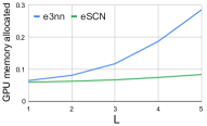
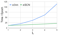
In Section 3, we showed our novel approach drastically reduces the cost of computing the tensor product. Here, we validate this claim by implementing two mathematically identical equivariat GNNs; one using e3nn PyTorch library (Geiger & Smidt, 2022) and the other one our efficient implementation. In Figure 1 we compare the GPU memory allocated at training time and the Time / Epoch over the maximal degree of the irreps. We conclude that our method can reduce the computational cost by an order of magnitude as we scale .
Additionally, we perform ablation studies across three variants of our model; varying the degree , the order , and the number of layers in Table 3. We see that energy MAE is more sensitive to the number of layers , while force MAE is more sensitive to the degree . We hypothesize this is due to the energy being more dependent on the entire structure’s configuration so more layers are helpful, while forces are more directionally dependent so high degrees of (higher directional resolution) are beneficial. Increasing improves results up to . Higher values may not increase accuracy since controls the resolution of the node representations perpendicular to the edges’ directions, which may be less useful to the network. Finally, we show results when the non-linear point-wise activation function, Equation (21), is removed from message passing (eSCN linear). We see accuracies decrease, but are still comparable to models with lower degrees or fewer layers.
The run times of the different model variations are also shown. Faster runtimes than those shown are possible for smaller models, if the batch sizes had been increased. Overall runtimes are similar to those of the SCN model.
7 Discussion
Research in atomic modeling is critical for addressing many of the world’s problems, especially with respect to our challenges with climate change. However, advances in chemistry can have both positive and negative impact as has been demonstrated in other chemistry breakthroughs. One cautionary example is the Haber-Bosch process (Hager, 2009) for ammonia production that enabled the world to feed itself, but has led to over fertilization and ocean dead zones. We hope to inspire positive uses by demonstrating our results on datasets such as OC20 (Chanussot et al., 2021).
The constraints imposed by the -equivariance not only limit the use of linear functions but also non-linearities. We utilize the point-wise spherical non-linearity since it is very expressive, as it processes the full spectrum of the spherical harmonics. Most other equivariant non-linear functions are applied to the norm of irreps and scalar coefficients. For point-wise spherical non-linearities the discrete transformation of the irreps to the sphere makes the operation quasi-equivariant and can be computationally expensive if equivariance to numerical precision is desired, Section D.
In conclusion, we unveil the relationship between and convolutions and how this can led to dramatic improvements in computational efficiency. We demonstrate the approach using our eSCN model that achieves state-of-the-art performance on atomic modeling tasks such as force prediction.
Acknowledgements
The authors thank Abhishek Das, Janice Lan, Brandon Wood, Mark Tygert and Gabriele Corso for valuable feedback and insightful discussions.
References
- Batatia et al. (2022) Batatia, I., Kovacs, D. P., Simm, G., Ortner, C., and Csányi, G. Mace: Higher order equivariant message passing neural networks for fast and accurate force fields. Advances in Neural Information Processing Systems, 35:11423–11436, 2022.
- Batzner et al. (2022) Batzner, S., Musaelian, A., Sun, L., Geiger, M., Mailoa, J. P., Kornbluth, M., Molinari, N., Smidt, T. E., and Kozinsky, B. E (3)-equivariant graph neural networks for data-efficient and accurate interatomic potentials. Nature communications, 13(1):1–11, 2022.
- Behler (2016) Behler, J. Perspective: Machine learning potentials for atomistic simulations. The Journal of chemical physics, 145(17):170901, 2016.
- Bocher (1906) Bocher, M. Introduction to the theory of fourier’s series. Annals of Mathematics, 7(3):81–152, 1906.
- Brandstetter et al. (2022) Brandstetter, J., Hesselink, R., van der Pol, E., Bekkers, E. J., and Welling, M. Geometric and physical quantities improve e(3) equivariant message passing. In International Conference on Learning Representations, 2022.
- Bronstein et al. (2021) Bronstein, M. M., Bruna, J., Cohen, T., and Veličković, P. Geometric deep learning: Grids, groups, graphs, geodesics, and gauges. arXiv preprint arXiv:2104.13478, 2021.
- Chanussot et al. (2021) Chanussot, L., Das, A., Goyal, S., Lavril, T., Shuaibi, M., Riviere, M., Tran, K., Heras-Domingo, J., Ho, C., Hu, W., Palizhati, A., Sriram, A., Wood, B., Yoon, J., Parikh, D., Zitnick, C. L., and Ulissi, Z. Open catalyst 2020 (oc20) dataset and community challenges. ACS Catalysis, 11(10):6059–6072, 2021.
- Chen et al. (2021) Chen, H., Liu, S., Chen, W., Li, H., and Hill, R. Equivariant point network for 3d point cloud analysis. In Proceedings of the IEEE/CVF conference on computer vision and pattern recognition, pp. 14514–14523, 2021.
- Chmiela et al. (2017) Chmiela, S., Tkatchenko, A., Sauceda, H. E., Poltavsky, I., Schütt, K. T., and Müller, K.-R. Machine learning of accurate energy-conserving molecular force fields. Science advances, 3(5):e1603015, 2017.
- Chmiela et al. (2018) Chmiela, S., Sauceda, H. E., Müller, K.-R., and Tkatchenko, A. Towards exact molecular dynamics simulations with machine-learned force fields. Nature communications, 9(1):1–10, 2018.
- Cohen & Welling (2016) Cohen, T. and Welling, M. Group equivariant convolutional networks. In International conference on machine learning, pp. 2990–2999. PMLR, 2016.
- Cohen & Welling (2017) Cohen, T. S. and Welling, M. Steerable CNNs. In International Conference on Learning Representations, 2017.
- Cohen et al. (2018) Cohen, T. S., Geiger, M., Köhler, J., and Welling, M. Spherical CNNs. In International Conference on Learning Representations, 2018.
- Deng et al. (2021) Deng, C., Litany, O., Duan, Y., Poulenard, A., Tagliasacchi, A., and Guibas, L. J. Vector neurons: A general framework for so (3)-equivariant networks. In Proceedings of the IEEE/CVF International Conference on Computer Vision, pp. 12200–12209, 2021.
- Elfwing et al. (2018) Elfwing, S., Uchibe, E., and Doya, K. Sigmoid-weighted linear units for neural network function approximation in reinforcement learning. Neural Networks, 107, 2018.
- Fuchs et al. (2020) Fuchs, F., Worrall, D., Fischer, V., and Welling, M. Se (3)-transformers: 3d roto-translation equivariant attention networks. Advances in Neural Information Processing Systems, 33:1970–1981, 2020.
- Gasteiger et al. (2020a) Gasteiger, J., Giri, S., Margraf, J. T., and Günnemann, S. Fast and uncertainty-aware directional message passing for non-equilibrium molecules. In NeurIPS-W, 2020a.
- Gasteiger et al. (2020b) Gasteiger, J., Groß, J., and Günnemann, S. Directional message passing for molecular graphs. In International Conference on Learning Representations (ICLR), 2020b.
- Gasteiger et al. (2021) Gasteiger, J., Becker, F., and Günnemann, S. Gemnet: Universal directional graph neural networks for molecules. Advances in Neural Information Processing Systems, 34:6790–6802, 2021.
- Gasteiger et al. (2022) Gasteiger, J., Shuaibi, M., Sriram, A., Günnemann, S., Ulissi, Z. W., Zitnick, C. L., and Das, A. Gemnet-oc: developing graph neural networks for large and diverse molecular simulation datasets. Transactions on Machine Learning Research, 2022.
- Geiger & Smidt (2022) Geiger, M. and Smidt, T. e3nn: Euclidean neural networks. arXiv preprint arXiv:2207.09453, 2022.
- Girshick et al. (2014) Girshick, R., Donahue, J., Darrell, T., and Malik, J. Rich feature hierarchies for accurate object detection and semantic segmentation. In Proceedings of the IEEE conference on computer vision and pattern recognition, 2014.
- González (2010) González, Á. Measurement of areas on a sphere using fibonacci and latitude–longitude lattices. Mathematical Geosciences, 42(1):49–64, 2010.
- Goodman & Wallach (2000) Goodman, R. and Wallach, N. R. Representations and invariants of the classical groups. 2000.
- Gori et al. (2005) Gori, M., Monfardini, G., and Scarselli, F. A new model for learning in graph domains. In Proceedings. 2005 IEEE international joint conference on neural networks, volume 2, pp. 729–734, 2005.
- Griffiths & Schroeter (2018) Griffiths, D. J. and Schroeter, D. F. Introduction to quantum mechanics. Cambridge university press, 2018.
- Hager (2009) Hager, T. The alchemy of air: a Jewish genius, a doomed tycoon, and the scientific discovery that fed the world but fueled the rise of Hitler. Broadway Books, 2009.
- Halgren (1996) Halgren, T. Merck molecular force field. i. basis, form, scope, parameterization, and performance of mmff94. Comput. Chem., 17:490–519, 1996.
- Hohenberg & Kohn (1964) Hohenberg, P. and Kohn, W. Inhomogeneous electron gas. Physical review, 136(3B):B864, 1964.
- Kipf & Welling (2017) Kipf, T. N. and Welling, M. Semi-supervised classification with graph convolutional networks. In International Conference on Learning Representations, 2017.
- Kohn & Sham (1965) Kohn, W. and Sham, L. J. Self-consistent equations including exchange and correlation effects. Physical review, 140(4A):A1133, 1965.
- Kondor et al. (2018) Kondor, R., Lin, Z., and Trivedi, S. Clebsch–gordan nets: a fully fourier space spherical convolutional neural network. Advances in Neural Information Processing Systems, 31, 2018.
- Lan et al. (2022) Lan, J., Palizhati, A., Shuaibi, M., Wood, B. M., Wander, B., Das, A., Uyttendaele, M., Zitnick, C. L., and Ulissi, Z. W. Adsorbml: Accelerating adsorption energy calculations with machine learning. arXiv preprint arXiv:2211.16486, 2022.
- Liao & Smidt (2023) Liao, Y.-L. and Smidt, T. Equiformer: Equivariant graph attention transformer for 3d atomistic graphs. In The Eleventh International Conference on Learning Representations, 2023.
- Liu et al. (2022) Liu, Y., Wang, L., Liu, M., Lin, Y., Zhang, X., Oztekin, B., and Ji, S. Spherical message passing for 3d molecular graphs. In International Conference on Learning Representations, 2022.
- Musaelian et al. (2023) Musaelian, A., Batzner, S., Johansson, A., Sun, L., Owen, C. J., Kornbluth, M., and Kozinsky, B. Learning local equivariant representations for large-scale atomistic dynamics. Nature Communications, 14(1):579, 2023.
- Poulenard & Guibas (2021) Poulenard, A. and Guibas, L. J. A functional approach to rotation equivariant non-linearities for tensor field networks. In Proceedings of the IEEE/CVF Conference on Computer Vision and Pattern Recognition, pp. 13174–13183, 2021.
- Puny et al. (2022) Puny, O., Atzmon, M., Smith, E. J., Misra, I., Grover, A., Ben-Hamu, H., and Lipman, Y. Frame averaging for invariant and equivariant network design. In International Conference on Learning Representations, 2022.
- Ramakrishnan et al. (2014) Ramakrishnan, R., Dral, P. O., Rupp, M., and Von Lilienfeld, O. A. Quantum chemistry structures and properties of 134 kilo molecules. Scientific data, 1(1):1–7, 2014.
- Reisert & Burkhardt (2009) Reisert, M. and Burkhardt, H. Spherical tensor calculus for local adaptive filtering. In Tensors in Image Processing and Computer Vision, pp. 153–178. Springer, 2009.
- Rolnick et al. (2022) Rolnick, D., Donti, P. L., Kaack, L. H., Kochanski, K., Lacoste, A., Sankaran, K., Ross, A. S., Milojevic-Dupont, N., Jaques, N., Waldman-Brown, A., et al. Tackling climate change with machine learning. ACM Computing Surveys (CSUR), 55(2):1–96, 2022.
- Satorras et al. (2021) Satorras, V. G., Hoogeboom, E., and Welling, M. E (n) equivariant graph neural networks. In International conference on machine learning. PMLR, 2021.
- Schrödinger (1926) Schrödinger, E. An undulatory theory of the mechanics of atoms and molecules. The Physical review, 28(6), 1926.
- Schütt et al. (2021) Schütt, K., Unke, O., and Gastegger, M. Equivariant message passing for the prediction of tensorial properties and molecular spectra. In International Conference on Machine Learning, pp. 9377–9388. PMLR, 2021.
- Schütt et al. (2018) Schütt, K. T., Sauceda, H. E., Kindermans, P.-J., Tkatchenko, A., and Müller, K.-R. Schnet–a deep learning architecture for molecules and materials. The Journal of Chemical Physics, 148(24):241722, 2018.
- Shuaibi et al. (2021) Shuaibi, M., Kolluru, A., Das, A., Grover, A., Sriram, A., Ulissi, Z., and Zitnick, C. L. Rotation invariant graph neural networks using spin convolutions. arXiv preprint arXiv:2106.09575, 2021.
- Thomas et al. (2018) Thomas, N., Smidt, T., Kearnes, S., Yang, L., Li, L., Kohlhoff, K., and Riley, P. Tensor field networks: Rotation-and translation-equivariant neural networks for 3d point clouds. arXiv preprint arXiv:1802.08219, 2018.
- Tran et al. (2023) Tran, R., Lan, J., Shuaibi, M., Wood, B. M., Goyal, S., Das, A., Heras-Domingo, J., Kolluru, A., Rizvi, A., Shoghi, N., et al. The open catalyst 2022 (oc22) dataset and challenges for oxide electrocatalysts. ACS Catalysis, 13(5):3066–3084, 2023.
- Wala & Klöckner (2020) Wala, M. and Klöckner, A. Optimization of fast algorithms for global quadrature by expansion using target-specific expansions. Journal of Computational Physics, 403:108976, 2020.
- Weiler et al. (2018) Weiler, M., Geiger, M., Welling, M., Boomsma, W., and Cohen, T. S. 3d steerable cnns: Learning rotationally equivariant features in volumetric data. Advances in Neural Information Processing Systems, 31, 2018.
- Weisstein (2003) Weisstein, E. W. Clebsch-gordan coefficient. 2003.
- Worrall et al. (2017) Worrall, D. E., Garbin, S. J., Turmukhambetov, D., and Brostow, G. J. Harmonic networks: Deep translation and rotation equivariance. In Proceedings of the IEEE Conference on Computer Vision and Pattern Recognition, pp. 5028–5037, 2017.
- Xie & Grossman (2018) Xie, T. and Grossman, J. C. Crystal graph convolutional neural networks for an accurate and interpretable prediction of material properties. Physical review letters, 120(14):145301, 2018.
- Zitnick et al. (2020) Zitnick, C. L., Chanussot, L., Das, A., Goyal, S., Heras-Domingo, J., Ho, C., Hu, W., Lavril, T., Palizhati, A., Riviere, M., Shuaibi, M., Sriram, A., Tran, K., Wood, B., Yoon, J., Parikh, D., and Ulissi, Z. An introduction to electrocatalyst design using machine learning for renewable energy storage. arXiv preprint arXiv:2010.09435, 2020.
- Zitnick et al. (2022) Zitnick, C. L., Das, A., Kolluru, A., Lan, J., Shuaibi, M., Sriram, A., Ulissi, Z. W., and Wood, B. M. Spherical channels for modeling atomic interactions. In Advances in Neural Information Processing Systems, 2022.
Appendix: Table of contents
Appendix A Proofs
A.1 Proof of Proposition 3.1
We start the proof noting that the Clebsch-Gordan coefficients used in the paper differ from the standard coefficients used in physics. The Clebsch-Gordan matrix used in quantum mechanics is the change-of-basis which decomposes the tensor product between irreducible representations. However, the irreps are related to the irreps as follows:
| (25) |
where is an irrep of degree and an irrep of degree .
Additionally, we denote the Clebsch-Gordan coefficients by . A well-known property (Weisstein, 2003) of is that they are non-zero only if and the following holds:
| (26) |
Therefore by substituting we obtain that is non-zero only if and the the following holds for any :
| (27) |
Now, we can relate the Clebsh-Gordan coefficients to the ones using a change-of-basis directly derived from Equation (25). We fix and note that the components of an irrep get rearranged to the components of an irrep as follows; for :
| (28) |
for :
| (29) |
Moreover , so for odd.
Additionally, we note that if implies that the same is true for .
We finally conclude that is non-zero only for , and and for any . Moreover, for any , when odd and when even; for , when odd.
This concludes the proof of the Proposition.
A.2 Proof that there exists a linear bijection between and
We start by noting that the Clebsch-Gordan coefficients are related to the ones with a linear invertible transformation. Therefore without loss of generality we can assume that are the ones used in quantum mechanics.
By definition, , which specifies a linear surjection from to for a fixed value of and .
We now prove that the aforementioned map from to is injective. Let’s suppose exists a set of such that for any . From Equation (14) we conclude that:
where is a 2D matrix which multiplies the vector . The above expression is for any value of which implies that the matrix is zero, therefore for any value of and :
| (30) |
Additionally, the Clebsch-Gordan coefficients satisfy the following properties (Weisstein, 2003); the first one is an orthogonality identity, the second one a permutation identity:
| (31) |
| (32) |
By taking the sum of Equation (30) over for a fixed value of we obtain:
| (33) |
where we substitute Equations (31) and (31) in the 5th and 4th equality. Therefore we conclude that for any value of , which implies that the linear map is injective.
We conclude the proof noting that a linear map between finite dimensional vector spaces which is both surjective and injective is bijective.
A.3 Proof of Theorem B.2
We first prove that there exists a projection map satisfying and for each . We note that, if we define in terms of as above, and we let to be the spaces then . We are left to prove that the representations are irreducible. A sufficient condition to prove it is to show that transforms like a circular harmonic of degree under the action . We note that this has already been proved in the main paper, which concludes the proof.
Lastly, we note that the projection map is invertible since, by definition, the linear change-of-basis map relating and is invertible.
Appendix B Mathematical foundations of and irreps
B.1 General introduction to equivariance
Group theory is a formalism to axiomatically define symmetries. A group is a set of elements with an operation which satisfies the following properties:
-
1.
There exists such that
-
2.
For all we have
-
3.
For all there exists such that
We can define infinitely many groups but the ones we are interested in are , the translation group, and most importantly , the rotation group of . The elements of should be regarded as rotations in and the group operation as the composition of rotations. In our context the symmetries transform a surrounding space: for this space is . Group action is a way to axiomatically define this operation. A group action on a vector space is an operation which satisfies:
-
1.
Exists such that
-
2.
we have
-
3.
we have
The canonical action of takes the symmetry (i.e. the rotation), an element of and rotates it accordingly.
Given two vector spaces (i.e. , for some and ) and a group , we say that is:
-
1.
-Invariant if
-
2.
-Equivariant if
In the OC-20 task the energy is invariant for both and , per-atom forces are invariant to and equivariant to .
B.2 Irreducible representations of SO(3) and SO(2)
We limit our study of symmetries to and , the group of 3D and 2D rotations, which are canonically acting on and . In this section, we classify how to extend the and action to other vector spaces for some integer .
We define the concept of group homomorphism to rephrase the the problem from another point of view. Given two groups we say is a group homomorphism if it satisfies .
We note that an action of a group on a vector space is mathematically equivalent to the existence of a group homomorphism where is the general linear group, the group of invertible matrices on . We define to be a representation of which acts as matrix multiplication on the vector space as follows:
| (34) |
Additionally, we define the concept of irreducible representations. Specifically, a representaion is reducible if there exists a non-trivial subspace such that , we have that ; otherwise we say the representation is irreducible.
We finally state the classification of the and irreducible representations.
For , only for odd there exists an irreducible representation . Moreover is unique up to a change of basis; we decide to remove the degeneracy arising from the possible change-of-basis by aligning the rotations’ generator to the y axis (as in the e3nn library). We define the Wigner- matrix of degree to be :
| (35) |
Therefore we let to be a dimensional vector space equipped with the action: the multiplication by a Wigner-D matrix. The elements of are called -irreps of degree .
Analogously, there exists a unique irreducible representation for , infinitely many for and none for . We enumerate the possible representations with an index where for and for and we define to be the irreducible representation indexed by . It satisfies
| (36) |
We define to be the vector space of the -irreps equipped with the action: the multiplication by the matrix of Equation 36.
B.3 Spherical and Circular Harmonics
The irreps have been intuitively defined starting from the first principles of symmetries. Nonetheless it can be hard to have intuition on the resulting space since we have added a few layers of abstraction. In this Section we introduce a way to build geometrical intuition by linking them to the spherical and circular harmonics.
The real spherical harmonic of degree is a function . The set of components of produces a basis for the homogeneous polynomial of degree on the sphere.
Analogously, the real circular harmonic of degree is a function , whose components produce a basis for the homogeneous polynomial of degree on the circle.
Most importantly they satisfy the following expressions:
| (37) |
We can make sense of a set of spherical harmonics by defining a function on the sphere such that . In this setting, acting on with a rotation matrix corresponds to rotating the frame of reference of the sphere. This shows that the -irreps can be treated as coefficients of the spherical harmonics. Analogously this is true for the -irreps and the circular harmonics on a circle.
B.4 Projection to SO(2)
Given an irreducible representation and a direction we define a projection as follows.
Definition B.1.
The projection of along is where is the subgroup of rotations around and is obtained by restricting the domain of the representation.
We reckon that is a representation of since is isomorphic to but it is not necessarily irreducible. Nonetheless, we can apply a change of basis and reduce it to
| (38) |
such that and is an irreducible representation of for any . This induces a projection map
| (39) |
We note that the projection map is unique up to the change of basis of . We provide in Theorem B.2 an explicit way to compute a projection map for and we prove that such a map is invertible.
Theorem B.2.
Let and then there exists a projection map such that , and for each
Moreover if then so that: and for each
Appendix C Computational comparison with e3nn tensor product
We study the computational advantage of our method from a theoretical point of view and we empirically validate our study.
We fix and study the computational complexity of a network with channels for each . The naive implementation calculates a tensor product for , and followed by a linear self-interaction expanding the number of channels of each degree back to . The number of tensor product operations scale with , each of which requires the computation of a 3D matrix multiplication; this accounts for operations. The tensor products are followed by linear self-interactions; they require the computation of matrices of dimension which accounts for operations. This becomes prohibitively expensive even with GPUs when we scale .
Our generalized convolutions can be efficiently parallelized in GPU by computing the matrix multiplications between and for . That is, we need 2D matrix multiplications to compute the full tensor product. This accounts for operations. Moreover we need an additional operations to rotate the various irreps to align the edge’s direction to the y-axis. A similar analysis shows that the GPU memory allocated at training time scales with for the formulation, whereas the naive implementation is .
In Figure 1, we empirically validate these results by comparing the training time per epoch and the GPU memory allocated at training time over . We fix the number of hidden channels to , remove any non-linearity in the network and train a pair of mathematically equivalent GNNs for .
Appendix D Analysis on the quasi-equivariance of the spherical activation function
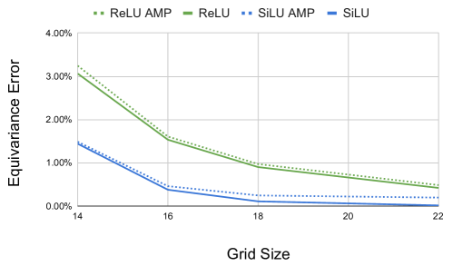
eSCN introduces non-linearities through a point-wise non-linearity described in Equations (21) and (22). (Cohen & Welling, 2016) proves that point-wise non-linearities are equivariant. However, the numerical approximation of the integration with a discrete number of samples results in a small loss of equivariance per-layer. Equation (21) is approximated by sampling points on a uniformly spaced grid along the directions with dimension . Equation (22) is sampled with resolution . If the activation function was linear, these resolutions would result in perfect equivariance. However, the higher frequencies introduced by a non-linear activation function can result in aliasing.
While not being perfectly equivariant, point-wise non-linearities have been adopted in many quasi-equivariant models, i.e., models with an equivariance error close to zero (Cohen et al., 2018). We study the equivariance error of the spherical activation of Equation (21) by varying the longitudinal and latitudinal grid size and the non-linear function employed. We measure the average percentage error between two rotated messages by:
| (40) |
where is a non-linear function chosen between and and the expectation is taken over uniformly sampled . For the settings used in this paper with a grid size of 14 with SiLU and AMP, only a small equivariance error () is observed. This error may be reduced below the level observable with AMP using a grid size of 18. Note that other activation functions that introduce more higher frequencies, such as ReLU, may require higher resolutions if numerically perfect equivariance is desired.
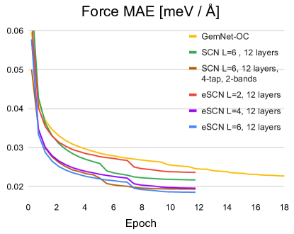
Appendix E Sample efficiency of eSCN
We provide an additional study on the sample efficiency of eSCN by empirically comparing it to state-of-the-art GemNet-OC (Gasteiger et al., 2022) and SCN (Zitnick et al., 2022). In Figure 10 we plot the Force MAE by training Epochs on the OC-20 2M (Chanussot et al., 2021) dataset. We conclude that eSCN preserves the same sample efficiency of SCN.